
D2L - 14.5. Multiscale Object Detection
2023. 8. 19. 19:59 |
https://d2l.ai/chapter_computer-vision/multiscale-object-detection.html
14.5. Multiscale Object Detection — Dive into Deep Learning 1.0.3 documentation
d2l.ai
14.5. Multiscale Object Detection
In Section 14.4, we generated multiple anchor boxes centered on each pixel of an input image. Essentially these anchor boxes represent samples of different regions of the image. However, we may end up with too many anchor boxes to compute if they are generated for every pixel. Think of a 561×728 input image. If five anchor boxes with varying shapes are generated for each pixel as their center, over two million anchor boxes (561×728×5) need to be labeled and predicted on the image.
섹션 14.4에서 입력 이미지의 각 픽셀을 중심으로 여러 앵커 상자를 생성했습니다. 기본적으로 이러한 앵커 상자는 이미지의 다른 영역 샘플을 나타냅니다. 그러나 앵커 상자가 모든 픽셀에 대해 생성되는 경우 계산하기에는 앵커 상자가 너무 많아질 수 있습니다. 561×728 입력 이미지를 생각해 보십시오. 각 픽셀마다 다양한 모양의 앵커 박스 5개를 중심으로 생성하면 200만 개가 넘는 앵커 박스(561×728×5)를 이미지에 라벨링하고 예측해야 합니다.
14.5.1. Multiscale Anchor Boxes
You may realize that it is not difficult to reduce anchor boxes on an image. For instance, we can just uniformly sample a small portion of pixels from the input image to generate anchor boxes centered on them. In addition, at different scales we can generate different numbers of anchor boxes of different sizes. Intuitively, smaller objects are more likely to appear on an image than larger ones. As an example, 1×1, 1×2, and 2×2 objects can appear on a 2×2 image in 4, 2, and 1 possible ways, respectively. Therefore, when using smaller anchor boxes to detect smaller objects, we can sample more regions, while for larger objects we can sample fewer regions.
이미지에서 앵커 박스를 줄이는 것이 어렵지 않다는 것을 알 수 있습니다. 예를 들어 입력 이미지에서 픽셀의 작은 부분을 균일하게 샘플링하여 중앙에 앵커 상자를 생성할 수 있습니다. 또한 크기가 다르면 크기가 다른 다양한 수의 앵커 박스를 생성할 수 있습니다. 직관적으로 작은 물체가 큰 물체보다 이미지에 나타날 가능성이 더 큽니다. 예를 들어, 1×1, 1×2, 2×2 객체는 각각 4, 2, 1가지 가능한 방식으로 2×2 이미지에 나타날 수 있습니다. 따라서 더 작은 앵커 상자를 사용하여 더 작은 객체를 감지할 때 더 많은 영역을 샘플링할 수 있는 반면 더 큰 객체의 경우 더 적은 영역을 샘플링할 수 있습니다.
To demonstrate how to generate anchor boxes at multiple scales, let’s read an image. Its height and width are 561 and 728 pixels, respectively.
여러 척도에서 앵커 상자를 생성하는 방법을 시연하기 위해 이미지를 읽어 보겠습니다. 높이와 너비는 각각 561픽셀과 728픽셀입니다.
%matplotlib inline
import torch
from d2l import torch as d2l

img = d2l.plt.imread('../img/catdog.jpg')
h, w = img.shape[:2]
h, w
(561, 728)위 코드는 이미지 파일을 로드하고 해당 이미지의 높이와 너비를 계산하는 부분입니다.
- %matplotlib inline: 이 코드는 Jupyter Notebook 등에서 Matplotlib 그림을 인라인으로 표시하도록 설정하는 명령입니다. Matplotlib을 사용하여 그래프나 이미지를 출력할 때 주피터 노트북 내에서 바로 볼 수 있게 합니다.
- import torch: 파이토치 라이브러리를 임포트합니다. 딥러닝과 텐서 연산을 위해 사용됩니다.
- from d2l import torch as d2l: d2l (Dive into Deep Learning) 라이브러리에서 파이토치에 대한 별칭을 d2l로 설정합니다. 이를 통해 d2l 라이브러리의 함수와 클래스를 이 코드에서 사용할 수 있게 됩니다.
- img = d2l.plt.imread('../img/catdog.jpg'): 이미지 파일을 읽어와 img 변수에 저장합니다. 이미지 파일의 경로는 ../img/catdog.jpg로 설정되어 있습니다. 해당 경로에 이미지 파일이 있어야 합니다.
- h, w = img.shape[:2]: 읽어온 이미지의 높이와 너비를 h와 w 변수에 저장합니다. .shape 속성을 사용하여 이미지의 형태를 확인하고, [:2] 슬라이싱을 통해 높이와 너비 정보만 추출합니다. 이렇게 함으로써 이미지의 높이와 너비를 h와 w 변수에 각각 할당합니다.
따라서 이 코드는 이미지 파일을 로드하고 해당 이미지의 높이와 너비를 확인하는 부분입니다.
Recall that in Section 7.2 we call a two-dimensional array output of a convolutional layer a feature map. By defining the feature map shape, we can determine centers of uniformly sampled anchor boxes on any image.
섹션 7.2에서 우리는 컨볼루션 레이어의 2차원 배열 출력을 피처 맵이라고 부릅니다. feature 맵 모양을 정의하여 모든 이미지에서 균일하게 샘플링된 앵커 박스의 중심을 결정할 수 있습니다.
The display_anchors function is defined below. We generate anchor boxes (anchors) on the feature map (fmap) with each unit (pixel) as the anchor box center. Since the (x,y)-axis coordinate values in the anchor boxes (anchors) have been divided by the width and height of the feature map (fmap), these values are between 0 and 1, which indicate the relative positions of anchor boxes in the feature map.
display_anchors 함수는 아래에 정의되어 있습니다. 각 단위(픽셀)를 앵커 상자 중심으로 하여 feature 맵(fmap)에 앵커 상자(앵커)를 생성합니다. 앵커 박스(anchor)의 (x,y)축 좌표 값을 특징 맵(fmap)의 너비와 높이로 나누었으므로 이 값은 0과 1 사이이며, 이것은 feature 맵에서 앵커 상자의 상대적 위치를 나타냅니다.
Since centers of the anchor boxes (anchors) are spread over all units on the feature map (fmap), these centers must be uniformly distributed on any input image in terms of their relative spatial positions. More concretely, given the width and height of the feature map fmap_w and fmap_h, respectively, the following function will uniformly sample pixels in fmap_h rows and fmap_w columns on any input image. Centered on these uniformly sampled pixels, anchor boxes of scale s (assuming the length of the list s is 1) and different aspect ratios (ratios) will be generated.
앵커 상자(앵커)의 중심은 기능 맵(fmap)의 모든 단위에 분산되어 있으므로 이러한 중심은 상대적인 공간 위치 측면에서 모든 입력 이미지에 균일하게 분포되어야 합니다. 보다 구체적으로, 기능 맵 fmap_w 및 fmap_h의 너비와 높이가 각각 주어지면 다음 함수는 모든 입력 이미지에서 fmap_h 행과 fmap_w 열의 픽셀을 균일하게 샘플링합니다. 이렇게 균일하게 샘플링된 픽셀을 중심으로 축척 s(목록 s의 길이가 1이라고 가정) 및 다른 종횡비(비율)의 앵커 상자가 생성됩니다.
def display_anchors(fmap_w, fmap_h, s):
    d2l.set_figsize()
    # Values on the first two dimensions do not affect the output
    fmap = torch.zeros((1, 10, fmap_h, fmap_w))
    anchors = d2l.multibox_prior(fmap, sizes=s, ratios=[1, 2, 0.5])
    bbox_scale = torch.tensor((w, h, w, h))
    d2l.show_bboxes(d2l.plt.imshow(img).axes,
                    anchors[0] * bbox_scale)
위 코드는 앵커 박스를 생성하고 시각적으로 표시하는 함수를 정의하는 부분입니다.
- def display_anchors(fmap_w, fmap_h, s):: display_anchors라는 함수를 정의합니다. 이 함수는 세 개의 인자를 받습니다: fmap_w, fmap_h, s.
- d2l.set_figsize(): 그래프의 크기를 설정하는 함수입니다. 이를 통해 플롯된 그림이 더 크게 표시될 수 있도록 설정합니다.
- fmap = torch.zeros((1, 10, fmap_h, fmap_w)): fmap은 4D 텐서로, 형태는 (1, 10, fmap_h, fmap_w)입니다. 첫 번째 차원은 배치 크기, 두 번째 차원은 채널 수, 세 번째와 네 번째 차원은 특징 맵의 높이와 너비입니다. 여기서 특징 맵의 값을 0으로 초기화합니다.
- anchors = d2l.multibox_prior(fmap, sizes=s, ratios=[1, 2, 0.5]): d2l.multibox_prior 함수를 사용하여 앵커 박스를 생성합니다. 이 함수는 입력으로 특징 맵, 앵커 박스의 크기(sizes), 앵커 박스의 종횡비(ratios)를 받습니다. fmap은 앞서 생성한 4D 텐서이며, sizes는 앵커 박스의 크기를 의미합니다. ratios는 앵커 박스의 종횡비를 나타냅니다.
- bbox_scale = torch.tensor((w, h, w, h)): bbox_scale은 이미지의 높이와 너비를 포함하는 1D 텐서입니다. 이미지의 너비와 높이를 통해 크기 조절에 사용됩니다.
- d2l.show_bboxes(d2l.plt.imshow(img).axes, anchors[0] * bbox_scale): d2l.show_bboxes 함수를 호출하여 앵커 박스를 이미지 위에 시각적으로 표시합니다. 이 함수는 두 개의 인자를 받습니다. 첫 번째 인자는 이미지가 그려질 축(axes)을 나타내며, 두 번째 인자는 앵커 박스의 좌표를 나타냅니다. 이 좌표를 bbox_scale로 크기를 조절한 뒤 앵커 박스를 시각적으로 표시합니다.
이 함수는 입력으로 주어진 특징 맵 크기와 앵커 박스의 크기, 종횡비를 활용하여 앵커 박스를 생성하고 시각적으로 표시하는 역할을 합니다.
First, let’s consider detection of small objects. In order to make it easier to distinguish when displayed, the anchor boxes with different centers here do not overlap: the anchor box scale is set to 0.15 and the height and width of the feature map are set to 4. We can see that the centers of the anchor boxes in 4 rows and 4 columns on the image are uniformly distributed.
먼저 작은 물체 감지에 대해 살펴보겠습니다. 표시할 때 쉽게 구별할 수 있도록 여기에서 중심이 다른 앵커 상자는 겹치지 않습니다. 앵커 상자 크기는 0.15로 설정되고 기능 맵의 높이와 너비는 4로 설정됩니다. 중심이 서로 다른 것을 볼 수 있습니다. 이미지에서 4행 4열의 앵커 상자가 균일하게 분포되어 있습니다.
display_anchors(fmap_w=4, fmap_h=4, s=[0.15])위 코드는 display_anchors 함수를 호출하여 특정한 파라미터로 앵커 박스를 생성하고 시각화하는 과정을 보여줍니다.
- display_anchors(fmap_w=4, fmap_h=4, s=[0.15]): display_anchors 함수를 호출하는 부분입니다. 함수에 세 개의 인자를 전달합니다. fmap_w는 특징 맵의 너비를, fmap_h는 특징 맵의 높이를, s는 앵커 박스의 크기를 의미하는 리스트를 전달합니다.
- fmap_w=4, fmap_h=4: 특징 맵의 너비와 높이를 각각 4로 설정합니다.
- s=[0.15]: 앵커 박스의 크기를 0.15로 설정합니다.
이렇게 설정된 파라미터로 display_anchors 함수가 호출되면, 해당 특징 맵과 앵커 박스의 크기를 활용하여 앵커 박스를 생성하고 이미지 위에 시각적으로 표시합니다. 이를 통해 특정 크기의 앵커 박스가 특정 위치에 어떻게 배치되는지를 확인할 수 있습니다.

We move on to reduce the height and width of the feature map by half and use larger anchor boxes to detect larger objects. When the scale is set to 0.4, some anchor boxes will overlap with each other.
계속해서 기능 맵의 높이와 너비를 절반으로 줄이고 더 큰 앵커 상자를 사용하여 더 큰 개체를 감지합니다. 배율을 0.4로 설정하면 일부 앵커 상자가 서로 겹칩니다.
display_anchors(fmap_w=2, fmap_h=2, s=[0.4])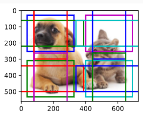
Finally, we further reduce the height and width of the feature map by half and increase the anchor box scale to 0.8. Now the center of the anchor box is the center of the image.
마지막으로 기능 맵의 높이와 너비를 절반으로 줄이고 앵커 상자 크기를 0.8로 늘립니다. 이제 앵커 상자의 중심이 이미지의 중심이 됩니다.
display_anchors(fmap_w=1, fmap_h=1, s=[0.8])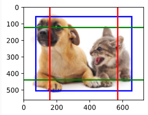
14.5.2. Multiscale Detection
Since we have generated multiscale anchor boxes, we will use them to detect objects of various sizes at different scales. In the following we introduce a CNN-based multiscale object detection method that we will implement in Section 14.7.
14.7. Single Shot Multibox Detection — Dive into Deep Learning 1.0.3 documentation
d2l.ai
멀티스케일 앵커 박스를 생성했으므로 이를 사용하여 다양한 스케일에서 다양한 크기의 객체를 감지할 것입니다. 다음에서는 14.7절에서 구현할 CNN 기반 멀티스케일 객체 감지 방법을 소개합니다.
At some scale, say that we have c feature maps of shape ℎ×w. Using the method in Section 14.5.1, we generate ℎw sets of anchor boxes, where each set has α anchor boxes with the same center. For example, at the first scale in the experiments in Section 14.5.1, given ten (number of channels) 4×4 feature maps, we generated 16 sets of anchor boxes, where each set contains 3 anchor boxes with the same center. Next, each anchor box is labeled with the class and offset based on ground-truth bounding boxes. At the current scale, the object detection model needs to predict the classes and offsets of ℎw sets of anchor boxes on the input image, where different sets have different centers.
어떤 규모에서 모양 ℎ×w의 특징 맵이 c개 있다고 가정해 보겠습니다. 섹션 14.5.1의 방법을 사용하여 ℎw 앵커 상자 세트를 생성합니다. 여기서 각 세트에는 동일한 중심을 가진 α 앵커 상자가 있습니다. 예를 들어 섹션 14.5.1 실험의 첫 번째 스케일에서 10개(채널 수)의 4×4 기능 맵이 주어졌을 때 우리는 16개의 앵커 상자 세트를 생성했으며 각 세트에는 동일한 중심을 가진 3개의 앵커 상자가 포함되어 있습니다. 다음으로, 각 앵커 상자는 실측 경계 상자를 기반으로 클래스 및 오프셋으로 레이블이 지정됩니다. 현재 규모에서 물체 감지 모델은 입력 이미지에서 앵커 상자의 ℎw 세트의 클래스와 오프셋을 예측해야 합니다. 여기서 세트마다 중심이 다릅니다.
Assume that the c feature maps here are the intermediate outputs obtained by the CNN forward propagation based on the input image. Since there are ℎw different spatial positions on each feature map, the same spatial position can be thought of as having c units. According to the definition of receptive field in Section 7.2, these c units at the same spatial position of the feature maps have the same receptive field on the input image: they represent the input image information in the same receptive field. Therefore, we can transform the c units of the feature maps at the same spatial position into the classes and offsets of the α anchor boxes generated using this spatial position. In essence, we use the information of the input image in a certain receptive field to predict the classes and offsets of the anchor boxes that are close to that receptive field on the input image.
여기서 c 특성 맵은 입력 이미지를 기반으로 CNN 정방향 전파에 의해 얻은 중간 출력이라고 가정합니다. 각 특징 맵에는 ℎw개의 서로 다른 공간 위치가 있으므로 동일한 공간 위치는 c 단위를 갖는 것으로 생각할 수 있습니다. 7.2 절의 수용 필드의 정의에 따르면, 특징 맵의 동일한 공간 위치에 있는 이러한 c 단위는 입력 이미지에서 동일한 수용 필드를 갖습니다. 즉, 동일한 수용 필드에서 입력 이미지 정보를 나타냅니다. 따라서 동일한 공간 위치에 있는 피처 맵의 c 단위를 이 공간 위치를 사용하여 생성된 α 앵커 상자의 클래스 및 오프셋으로 변환할 수 있습니다. 본질적으로 우리는 입력 이미지의 수용 필드에 가까운 앵커 박스의 클래스와 오프셋을 예측하기 위해 특정 수용 필드의 입력 이미지 정보를 사용합니다.
When the feature maps at different layers have varying-size receptive fields on the input image, they can be used to detect objects of different sizes. For example, we can design a neural network where units of feature maps that are closer to the output layer have wider receptive fields, so they can detect larger objects from the input image.
다른 레이어의 기능 맵이 입력 이미지에 다양한 크기의 수용 필드를 가지고 있는 경우 다양한 크기의 객체를 감지하는 데 사용할 수 있습니다. 예를 들어 출력 레이어에 더 가까운 기능 맵 단위가 더 넓은 수용 필드를 갖는 신경망을 설계하여 입력 이미지에서 더 큰 객체를 감지할 수 있습니다.
In a nutshell, we can leverage layerwise representations of images at multiple levels by deep neural networks for multiscale object detection. We will show how this works through a concrete example in Section 14.7.
간단히 말해서, 우리는 다중 규모 객체 감지를 위해 심층 신경망에 의해 여러 수준에서 이미지의 계층적 표현을 활용할 수 있습니다. 섹션 14.7에서 구체적인 예를 통해 이것이 어떻게 작동하는지 보여줄 것입니다.
14.5.3. Summary
- At multiple scales, we can generate anchor boxes with different sizes to detect objects with different sizes.
다양한 규모에서 다양한 크기의 앵커 박스를 생성하여 다양한 크기의 물체를 감지할 수 있습니다. - By defining the shape of feature maps, we can determine centers of uniformly sampled anchor boxes on any image.
특징 맵의 모양을 정의함으로써 모든 이미지에서 균일하게 샘플링된 앵커 박스의 중심을 결정할 수 있습니다. - We use the information of the input image in a certain receptive field to predict the classes and offsets of the anchor boxes that are close to that receptive field on the input image.
특정 수용 필드의 입력 이미지 정보를 사용하여 입력 이미지의 해당 수용 필드에 가까운 앵커 박스의 클래스와 오프셋을 예측합니다. - Through deep learning, we can leverage its layerwise representations of images at multiple levels for multiscale object detection.
딥 러닝을 통해 멀티스케일 객체 감지를 위해 여러 수준에서 이미지의 레이어별 표현을 활용할 수 있습니다.
14.5.4. Exercises
- According to our discussions in Section 8.1, deep neural networks learn hierarchical features with increasing levels of abstraction for images. In multiscale object detection, do feature maps at different scales correspond to different levels of abstraction? Why or why not?
- At the first scale (fmap_w=4, fmap_h=4) in the experiments in Section 14.5.1, generate uniformly distributed anchor boxes that may overlap.
- Given a feature map variable with shape 1×c×ℎ×w, where c, ℎ, and w are the number of channels, height, and width of the feature maps, respectively. How can you transform this variable into the classes and offsets of anchor boxes? What is the shape of the output?
'Dive into Deep Learning > D2L Computer Vision' 카테고리의 다른 글
| D2L - 14.10. Transposed Convolution (1) | 2023.08.21 |
|---|---|
| D2L - 14.9. Semantic Segmentation and the Dataset (0) | 2023.08.20 |
| D2L - 14.8. Region-based CNNs (R-CNNs) (0) | 2023.08.20 |
| D2L - 14.7. Single Shot Multibox Detection (0) | 2023.08.19 |
| D2L - 14.6. The Object Detection Dataset (0) | 2023.08.19 |
| D2L - 14.4. Anchor Boxes (0) | 2023.08.19 |
| D2L - 14.3. Object Detection and Bounding Boxes (0) | 2023.08.19 |
| D2L - 14.2. Fine-Tuning (0) | 2023.08.19 |
| D2L - 14.1. Image Augmentation (0) | 2023.08.19 |
| D2L - 14. Computer Vision (0) | 2023.08.18 |