https://d2l.ai/chapter_attention-mechanisms-and-transformers/large-pretraining-transformers.html

11.9. Large-Scale Pretraining with Transformers

So far in our image classification and machine translation experiments, models were trained on datasets with input-output examples from scratch to perform specific tasks. For example, a Transformer was trained with English-French pairs (Section 11.7) so that this model can translate input English text into French. As a result, each model becomes a specific expert that is sensitive to even slight shift in data distribution (Section 4.7). For better generalized models, or even more competent generalists that can perform multiple tasks with or without adaptation, pretraining models on large data has been increasingly common.

지금까지 이미지 분류 및 기계 번역 실험에서 모델은 특정 작업을 수행하기 위해 처음부터 입력-출력 예제가 있는 데이터 세트에 대해 훈련되었습니다. 예를 들어 Transformer는 이 모델이 입력 영어 텍스트를 프랑스어로 번역할 수 있도록 영어-프랑스어 쌍(섹션 11.7)으로 훈련되었습니다. 결과적으로 각 모델은 데이터 분포의 약간의 변화에도 민감한 특정 전문가가 됩니다(섹션 4.7). 더 나은 일반화 모델 또는 적응 여부에 관계없이 여러 작업을 수행할 수 있는 더 유능한 제너럴리스트를 위해 대용량 데이터에 대한 모델 사전 훈련이 점점 보편화되었습니다.

Given larger data for pretraining, the Transformer architecture performs better with an increased model size and training compute, demonstrating superior scaling behavior. Specifically, performance of Transformer-based language models scales as a power-law with the amount of model parameters, training tokens, and training compute (Kaplan et al., 2020). The scalability of Transformers is also evidenced by the significantly boosted performance from larger vision Transformers trained on larger data (discussed in Section 11.8). More recent success stories include Gato, a generalist model that can play Atari, caption images, chat, and act as a robot (Reed et al., 2022). Gato is a single Transformer that scales well when pretrained on diverse modalities, including text, images, joint torques, and button presses. Notably, all such multi-modal data is serialized into a flat sequence of tokens, which can be processed akin to text tokens (Section 11.7) or image patches (Section 11.8) by Transformers.

사전 교육을 위한 더 큰 데이터가 주어지면 Transformer 아키텍처는 모델 크기와 교육 컴퓨팅이 증가하여 더 나은 성능을 발휘하여 우수한 확장 동작을 보여줍니다. 특히 Transformer 기반 언어 모델의 성능은 모델 매개변수, 교육 토큰 및 교육 컴퓨팅의 양에 따라 power-law으로 확장됩니다(Kaplan et al., 2020). Transformers의 확장성은 또한 더 큰 데이터에 대해 훈련된 더 큰 비전 Transformers의 성능이 크게 향상된 것으로 입증됩니다(11.8절에서 설명). 보다 최근의 성공 사례로는 Atari를 플레이하고, 이미지에 캡션을 달고, 채팅하고, 로봇 역할을 할 수 있는 일반 모델인 Gato가 있습니다(Reed et al., 2022). Gato는 텍스트, 이미지, 조인트 토크 및 버튼 누름을 비롯한 다양한 양식에 대해 사전 훈련되었을 때 잘 확장되는 단일 Transformer입니다. 특히 이러한 모든 다중 모달 데이터는 트랜스포머에 의해 텍스트 토큰(11.7절) 또는 이미지 패치(11.8절)와 유사하게 처리될 수 있는 토큰의 플랫 시퀀스로 직렬화됩니다.

Power-law 란?

The power-law, also known as a power-law distribution or scaling law, refers to a mathematical relationship between two quantities in which one quantity's value is proportional to a power of the other. In other words, a power-law distribution describes a relationship where the frequency of an event (or the occurrence of a value) decreases rapidly as the event becomes more frequent or the value becomes larger.

'Power-law', 또는 'power-law 분포' 또는 'scaling law'는 두 quantities  사이의 수학적 관계를 나타내며, 한 quantity 의 값이 다른 quantity 의 거듭제곱에 비례하는 관계를 의미합니다. 다시 말해, power-law 분포는 어떤 사건의 빈도(또는 값의 발생)가 해당 사건이 더 자주 발생하거나 값이 더 크면 빠르게 감소하는 관계를 설명합니다.

Mathematically, a power-law relationship can be expressed as:

수학적으로 power-law 관계는 다음과 같이 표현할 수 있습니다:

P(x)∝x−α

Here, P(x) represents the probability or frequency of the event or value x, and α is the exponent that determines the rate of decrease. A smaller value of α leads to a slower decrease, while a larger value of α leads to a faster decrease.

여기서 P(x)는 사건 또는 값 x의 확률 또는 빈도를 나타내며, α는 감소율을 결정하는 지수입니다. α 값이 작을수록 감소가 느리게 진행되며, α 값이 클수록 빠르게 감소합니다.

Power-law distributions are common in various natural, social, and economic systems. They are characterized by a few highly frequent events or values (often referred to as "hubs" or "outliers") and many less frequent events or values. This distribution is also known as a "long-tailed" distribution because the tail of the distribution extends over a wide range of values.

Power-law 분포는 자연, 사회, 경제 시스템에서 일반적으로 나타나며, 몇 개의 높은 빈도 사건 또는 값(일반적으로 "허브" 또는 "아웃라이어"로 불림)과 많은 낮은 빈도 사건 또는 값이 특징입니다. 이 분포는 종종 "긴 꼬리" 분포로 알려져 있습니다. 분포의 꼬리 부분이 넓은 범위의 값을 포함하기 때문입니다.

Examples of phenomena that exhibit power-law distributions include the distribution of income, city sizes, word frequencies in texts, earthquake magnitudes, and the number of links in online networks like the Internet. The study of power-law distributions is essential in understanding the behavior and dynamics of complex systems and networks.

수입 분포, 도시 규모, 텍스트에서의 단어 빈도, 지진 규모, 인터넷과 같은 온라인 네트워크의 링크 수 등 다양한 자연, 사회 및 경제 현상에서 power-law 분포가 나타납니다. power-law 분포의 연구는 복잡한 시스템과 네트워크의 동작과 역학을 이해하는 데 중요합니다.

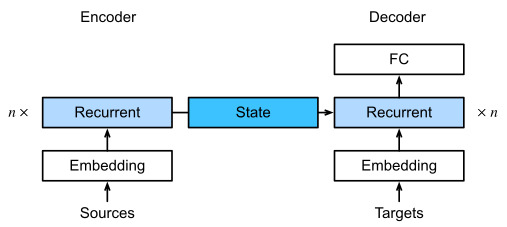
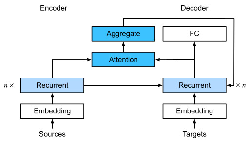
Before compelling success of pretraining Transformers for multi-modal data, Transformers were extensively pretrained with a wealth of text. Originally proposed for machine translation, the Transformer architecture in Fig. 11.7.1 consists of an encoder for representing input sequences and a decoder for generating target sequences. Primarily, Transformers can be used in three different modes: encoder-only, encoder-decoder, and decoder-only. To conclude this chapter, we will review these three modes and explain the scalability in pretraining Transformers.

multi-modal data에 대한 Transformers의 사전 교육이 성공하기 전에 Transformers는 풍부한 텍스트로 광범위하게 사전 교육을 받았습니다. 원래 기계 번역을 위해 제안된 그림 11.7.1의 Transformer 아키텍처는 입력 시퀀스를 나타내는 인코더와 대상 시퀀스를 생성하는 디코더로 구성됩니다. 기본적으로 트랜스포머는 encoder-only, encoder-decoder, and decoder-only 의 세 가지 모드로 사용할 수 있습니다. 이 장을 마무리하기 위해 이 세 가지 모드를 검토하고 Transformer를 사전 훈련할 때의 확장성을 설명합니다.

Multi Modal 이란?

'Multi-modal'은 여러 가지 다른 형태, 유형 또는 모드가 함께 존재하는 상황이나 시스템을 나타내는 용어입니다. 이 용어는 다양한 정보나 자료 소스가 혼합되어 하나의 전체를 구성하는 경우를 가리킵니다. 다른 말로 하면, 다양한 모드나 형태가 복합적으로 존재하여 상호작용하거나 조합되는 상황을 말합니다.

예를 들어, 'multi-modal data'는 여러 유형의 데이터가 함께 존재하는 경우를 의미합니다. 이러한 데이터는 텍스트, 이미지, 음성 등 다양한 형식의 정보를 포함할 수 있습니다. 머신러닝이나 딥러닝 분야에서 'multi-modal learning'은 여러 종류의 데이터로부터 모델을 학습시키는 기술을 의미합니다. 이러한 방식으로 학습된 모델은 다양한 유형의 정보를 통합하여 더 풍부한 표현을 생성하거나 복잡한 문제를 해결하는 데 사용될 수 있습니다.

또한 'multi-modal'은 감각적인 정보나 경험의 다양성을 나타낼 때도 사용될 수 있습니다. 예를 들어, 'multi-modal perception'은 시각, 청각, 후각, 촉각 등 다양한 감각 정보를 통해 환경을 인식하는 능력을 의미합니다.

BERT란?

BERT, which stands for "Bidirectional Encoder Representations from Transformers," is a revolutionary pre-trained language model developed by Google AI (Google Research) in 2018. BERT has significantly advanced the field of natural language processing (NLP) and has had a profound impact on various NLP tasks.

BERT는 "Bidirectional Encoder Representations from Transformers"의 약자로, 2018년 Google AI(구글 연구소)에서 개발한 혁신적인 사전 훈련 언어 모델입니다. BERT는 자연어 처리(NLP) 분야를 혁신하며 다양한 NLP 작업에 깊은 영향을 미쳤습니다.

Here are some key features and concepts related to BERT:

다음은 BERT에 관련한 주요 기능과 개념입니다:

1. Transformer Architecture: BERT is built upon the Transformer architecture, which is a type of neural network architecture specifically designed for handling sequences of data, such as sentences or paragraphs. The Transformer architecture incorporates self-attention mechanisms that allow it to capture contextual relationships among words in a sentence.
   
   트랜스포머 아키텍처: BERT는 트랜스포머 아키텍처를 기반으로 구축되었으며, 문장이나 단락과 같은 시퀀스 데이터를 처리하는 데 특화된 신경망 아키텍처입니다. 트랜스포머 아키텍처는 self-attention 메커니즘을 포함하며 문장 내 단어 간의 문맥 관계를 파악할 수 있습니다.
   
   
2. Bidirectional Context: One of the most important features of BERT is that it's bidirectional, meaning it reads text in both directions (left-to-right and right-to-left) during training. This allows the model to have a better understanding of the context in which a word appears.
   
   양방향 문맥: BERT의 가장 중요한 특징 중 하나는 양방향입니다. 이는 모델이 학습 중에 텍스트를 양방향(왼쪽에서 오른쪽으로, 오른쪽에서 왼쪽으로)으로 읽는다는 것을 의미합니다. 이로써 모델은 단어가 문맥 내에서 어떻게 나타나는지에 대한 더 나은 이해를 갖게 됩니다.
   
   
3. Pre-training and Fine-tuning: BERT is pre-trained on a massive amount of text data using two unsupervised tasks: masked language modeling and next sentence prediction. In masked language modeling, random words in a sentence are masked, and the model is trained to predict those masked words. In next sentence prediction, the model learns to predict whether two sentences follow each other logically.
   
   사전 훈련 및 세부 조정: BERT는 무언어 학습 작업 중 두 가지 비지도 작업인 마스크된 언어 모델링과 다음 문장 예측으로 대량의 텍스트 데이터에 사전 훈련됩니다. 마스크된 언어 모델링에서 문장 내의 무작위 단어가 마스크되고, 모델은 해당 마스크된 단어를 예측하도록 훈련됩니다. 다음 문장 예측에서는 두 문장이 논리적으로 이어지는지를 예측하는 방식으로 학습합니다.
   
   
4. Contextualized Word Representations: BERT generates contextualized word representations, which means that the representation of a word depends on its surrounding words in a sentence. This allows the model to capture various nuances and polysemy in language.
   
   문맥화된 단어 표현: BERT는 문맥화된 단어 표현을 생성하며, 단어의 표현이 문장 내 주변 단어에 따라 다릅니다. 이를 통해 모델은 언어의 다양한 뉘앙스와 일어날 수 있는 다의성을 포착할 수 있습니다.
   
   
5. Transfer Learning: BERT's pre-trained model can be fine-tuned on specific downstream tasks with smaller amounts of task-specific data. This transfer learning approach has been shown to yield impressive results on a wide range of NLP tasks, such as text classification, named entity recognition, question answering, sentiment analysis, and more.
   
   전이 학습: BERT의 사전 훈련된 모델은 작은 양의 과제 특화 데이터로 세부적인 다운스트림 작업에 대해 세밀하게 조정될 수 있습니다. 이러한 전이 학습 방식은 다양한 NLP 작업(텍스트 분류, 개체명 인식, 질문 응답, 감정 분석 등)에서 놀라운 결과를 얻을 수 있도록 해주었습니다.
   
   
6. Transformer Layers: BERT consists of multiple layers of Transformer encoders. Each layer processes the input sequence and passes it through self-attention mechanisms and feed-forward neural networks, enhancing the model's ability to capture complex relationships.
   
   트랜스포머 레이어: BERT는 여러 개의 트랜스포머 인코더 레이어로 구성됩니다. 각 레이어는 입력 시퀀스를 처리하고 자기 어텐션 메커니즘과 피드포워드 신경망을 통과시켜 복잡한 관계를 포착하는 능력을 향상시킵니다.
   
   
7. Large Scale: BERT was initially released in two versions: BERT-base and BERT-large. The "large" version has more parameters and is capable of capturing more nuanced patterns in the text but requires more computational resources.
   
   대규모 규모: BERT는 초기에 BERT-base와 BERT-large 두 가지 버전으로 출시되었습니다. "large" 버전은 매개변수가 더 많고 텍스트 내에서 더 미묘한 패턴을 포착할 수 있지만, 더 많은 컴퓨팅 자원이 필요합니다.
   
   
8. Contextualized Word Embeddings: BERT produces contextualized word embeddings, which are highly useful for downstream tasks. These embeddings capture not only syntactic information but also semantic relationships between words.
   
   문맥화된 단어 임베딩: BERT는 문맥화된 단어 임베딩을 생성하며, 이는 하위 작업에 매우 유용합니다. 이러한 임베딩은 구문 정보 뿐만 아니라 단어 간의 의미적 관계를 포착합니다.
   
   

BERT's success has led to the development of various other transformer-based models like GPT (Generative Pre-trained Transformer), RoBERTa, XLNet, and more. These models have achieved state-of-the-art results on a wide array of NLP benchmarks and continue to drive advancements in the field.

BERT의 성공은 GPT(Generative Pre-trained Transformer), RoBERTa, XLNet 등과 같은 다양한 트랜스포머 기반 모델의 개발을 이끌었습니다. 이러한 모델은 다양한 NLP 벤치마크에서 최첨단 결과를 달성하고, 계속해서 이 분야의 발전을 주도하고 있습니다.

11.9.1. Encoder-Only

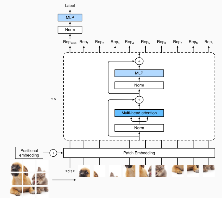
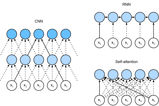
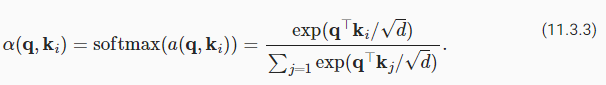
When only the Transformer encoder is used, a sequence of input tokens is converted into the same number of representations that can be further projected into output (e.g., classification). A Transformer encoder consists of self-attention layers, where all input tokens attend to each other. For example, vision Transformers depicted in Fig. 11.8.1 are encoder-only, converting a sequence of input image patches into the representation of a special “<cls>” token. Since this representation depends on all input tokens, it is further projected into classification labels. This design was inspired by an earlier encoder-only Transformer pretrained on text: BERT (Bidirectional Encoder Representations from Transformers) (Devlin et al., 2018).

Transformer encoder만 사용되는 경우 입력 토큰 시퀀스는 출력(예: 분류)으로 추가로 투영될 수 있는 동일한 수의 representations 으로 변환됩니다. Transformer 인코더는 모든 입력 토큰이 서로 attend 하는 self-attention layers으로 구성됩니다. 예를 들어 그림 11.8.1에 묘사된 비전 트랜스포머는 인코더 전용이며 일련의 입력 이미지 패치를 특수 "<cls>" 토큰의 representation 으로 변환합니다. 이 representation 은 모든 입력 토큰에 따라 달라지므로 분류 레이블에 추가로 투영됩니다. 이 디자인은 BERT(Bidirectional Encoder Representations from Transformers)(Devlin et al., 2018)라는 텍스트로 사전 훈련된 초기 인코더 전용 Transformer에서 영감을 받았습니다.

11.9.1.1. Pretraining BERT

BERT is pretrained on text sequences using masked language modeling: input text with randomly masked tokens is fed into a Transformer encoder to predict the masked tokens. As illustrated in Fig. 11.9.1, an original text sequence “I”, “love”, “this”, “red”, “car” is prepended with the “<cls>” token, and the “<mask>” token randomly replaces “love”; then the cross-entropy loss between the masked token “love” and its prediction is to be minimized during pretraining. Note that there is no constraint in the attention pattern of Transformer encoders (right of Fig. 11.9.1) so all tokens can attend to each other. Thus, prediction of “love” depends on input tokens before and after it in the sequence. This is why BERT is a “bidirectional encoder”. Without need for manual labeling, large-scale text data from books and Wikipedia can be used for pretraining BERT.

BERT는 masked language modeling을 사용하여 텍스트 시퀀스에 대해 사전 학습된 모델입니다. 임의로 마스킹된 토큰이 있는 입력 텍스트는 masked tokens을 예측하기 위해 Transformer 인코더에 공급됩니다. 그림 11.9.1과 같이 원본 텍스트 시퀀스 "I", "love", "this", "red", "car" 앞에 "<cls>" 토큰이 추가되고 "<mask>" 토큰은 무작위로 "love"을 대체합니다. 그런 다음 마스킹된 토큰 "사랑"과 그 예측 사이의 교차 엔트로피 손실은 사전 훈련 중에 최소화됩니다. Transformer 인코더(그림 11.9.1의 오른쪽)의 attention  패턴에는 제약이 없으므로 모든 토큰이 서로 attend 할 수 있습니다. 따라서 "love"의 예측은 시퀀스에서 전후의 입력 토큰에 따라 달라집니다. 이것이 BERT가 "양방향 인코더 bidirectional encoder"인 이유입니다. 수동 레이블 지정이 필요 없이 책과 Wikipedia의 대규모 텍스트 데이터를 BERT 사전 학습에 사용할 수 있습니다.

11.9.1.2. Fine-Tuning BERT

The pretrained BERT can be fine-tuned to downstream encoding tasks involving single text or text pairs. During fine-tuning, additional layers can be added to BERT with randomized parameters: these parameters and those pretrained BERT parameters will be updated to fit training data of downstream tasks.

사전 훈련된 BERT는 단일 텍스트 또는 텍스트 쌍을 포함하는 다운스트림 인코딩 작업으로 미세 조정fine-tuned 할 수 있습니다. 미세 조정 중에 무작위 매개변수를 사용하여 추가 계층을 BERT에 추가할 수 있습니다. 이러한 매개변수와 사전 훈련된 BERT 매개변수는 다운스트림 작업의 훈련 데이터에 맞게 업데이트됩니다.

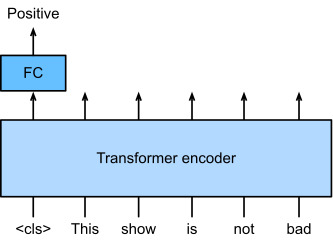
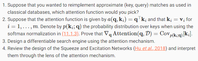
Fig. 11.9.2 illustrates fine-tuning of BERT for sentiment analysis. The Transformer encoder is a pretrained BERT, which takes a text sequence as input and feeds the “<cls>” representation (global representation of the input) into an additional fully connected layer to predict the sentiment. During fine-tuning, the cross-entropy loss between the prediction and the label on sentiment analysis data is minimized via gradient-based algorithms, where the additional layer is trained from scratch while pretrained parameters of BERT are updated. BERT does more than sentiment analysis. The general language representations learned by the 350-million-parameter BERT from 250 billion training tokens advanced the state of the art for natural language tasks such as single text classification, text pair classification or regression, text tagging, and question answering.

그림 11.9.2는 감정 분석을 위한 BERT의 미세 조정을 보여줍니다. 트랜스포머 인코더는 사전 훈련된 BERT로, 텍스트 시퀀스를 입력으로 취하고 "<cls>" 표현(입력의 전역 표현)을 완전히 연결된 추가 레이어에 공급하여 감정을 예측합니다. 미세 조정 중에 감정 분석 데이터의 예측과 레이블 간의 교차 엔트로피 손실은 그래디언트 기반 알고리즘을 통해 최소화됩니다. 여기서 추가 레이어는 처음부터 훈련되고 BERT의 사전 훈련된 매개변수는 업데이트됩니다. BERT는 감정 분석 이상의 기능을 수행합니다. 2,500억 개의 훈련 토큰에서 3억 5천만 개의 매개변수 BERT가 학습한 일반 언어 표현은 단일 텍스트 분류, 텍스트 쌍 분류 또는 회귀, 텍스트 태깅 및 질문 응답과 같은 자연어 작업을 위한 최신 기술을 발전시켰습니다.

You may note that these downstream tasks include text pair understanding. BERT pretraining has another loss for predicting whether one sentence immediately follows the other. However, this loss was later found not useful when pretraining RoBERTa, a BERT variant of the same size, on 2000 billion tokens (Liu et al., 2019). Other derivatives of BERT improved model architectures or pretraining objectives, such as ALBERT (enforcing parameter sharing) (Lan et al., 2019), SpanBERT (representing and predicting spans of text) (Joshi et al., 2020), DistilBERT (lightweight via knowledge distillation) (Sanh et al., 2019), and ELECTRA (replaced token detection) (Clark et al., 2020). Moreover, BERT inspired Transformer pretraining in computer vision, such as with vision Transformers (Dosovitskiy et al., 2021), Swin Transformers (Liu et al., 2021), and MAE (masked autoencoders) (He et al., 2022).

이러한 다운스트림 작업에는 텍스트 쌍 이해가 포함되어 있음을 알 수 있습니다. BERT 사전 훈련은 한 문장이 다른 문장 바로 뒤에 오는지 예측하는 데 또 다른 손실이 있습니다. 그러나 이 손실은 나중에 동일한 크기의 BERT 변형인 RoBERTa를 20000억 개(2조개?)의 토큰으로 사전 훈련할 때 유용하지 않은 것으로 밝혀졌습니다(Liu et al., 2019). ALBERT(매개 변수 공유 적용)(Lan et al., 2019), SpanBERT(텍스트 범위 표현 및 예측)(Joshi et al., 2020), DistilBERT(lightweight via 지식 증류)(Sanh et al., 2019) 및 ELECTRA(대체 토큰 탐지)(Clark et al., 2020). 또한 BERT는 비전 Transformers(Dosovitskiy et al., 2021), Swin Transformers(Liu et al., 2021) 및 MAE(masked autoencoders)(He et al., 2022)와 같은 컴퓨터 비전의 Transformer 사전 훈련에 영감을 주었습니다.

11.9.2. Encoder-Decoder

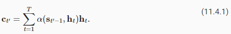
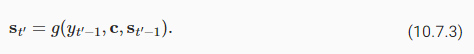
Since a Transformer encoder converts a sequence of input tokens into the same number of output representations, the encoder-only mode cannot generate a sequence of arbitrary length like in machine translation. As originally proposed for machine translation, the Transformer architecture can be outfitted with a decoder that autoregressively predicts the target sequence of arbitrary length, token by token, conditional on both encoder output and decoder output: (i) for conditioning on encoder output, encoder-decoder cross-attention (multi-head attention of decoder in Fig. 11.7.1) allows target tokens to attend to all input tokens; (ii) conditioning on decoder output is achieved by a so-called causal attention (this name is common in the literature but is misleading as it has little connection to the proper study of causality) pattern (masked multi-head attention of decoder in Fig. 11.7.1), where any target token can only attend to past and present tokens in the target sequence.

Transformer 인코더는 일련의 입력 토큰을 동일한 수의 출력 표현으로 변환하므로 인코더 전용 모드는 기계 번역과 같이 임의 길이의 시퀀스를 생성할 수 없습니다. 원래 기계 번역을 위해 제안된 것처럼 Transformer 아키텍처에는 인코더 출력과 디코더 출력 모두에 조건부로 토큰별로 임의 길이의 대상 시퀀스를 자동 회귀적으로 예측하는 디코더가 장착될 수 있습니다.(i) encoder-decoder cross-attention (그림 11.7.1의 디코더의 multi-head attention)는 대상 토큰이 모든 입력 토큰에 attend 하도록 허용합니다. (ii) 디코더 출력에 대한 컨디셔닝은 소위 causal attention(이 이름은 문헌에서 일반적이지만 causal  관계에 대한 적절한 연구와 거의 관련이 없기 때문에 오해의 소지가 있음) 패턴(그림에서 디코더의 마스킹된 다중 헤드 주의)에 의해 달성됩니다. . 11.7.1), 대상 토큰은 대상 시퀀스의 과거 및 현재 토큰에만 attend 할 수 있습니다.

Casual Attention이란?

"Casual Attention"은 주로 시계열 데이터와 같이 순차적인 시간 또는 순서적인 관계를 가진 데이터에서 사용되는 어텐션 메커니즘입니다. 이러한 어텐션은 현재 위치 이전의 시점들만을 참조하여 예측하거나 분석하는 데 사용됩니다.

일반적으로 어텐션 메커니즘은 현재 위치의 쿼리(Query)와 모든 위치의 키(Key) 및 값(Value)을 사용하여 가중 평균을 계산하는데, 이 때문에 시계열 데이터와 같이 순서가 중요한 데이터에서 미래의 정보가 과도하게 유출될 수 있습니다. 이러한 문제를 해결하기 위해 "Casual Attention"은 현재 시점 이후의 정보에 대한 접근을 막음으로써 미래 정보의 유출을 방지합니다.

보통 "Casual Attention"은 마스크(mask)를 사용하여 현재 시점 이후의 위치를 가리고, 오직 현재 시점 이전의 위치만을 참조하도록 제한합니다. 이로써 모델은 현재 시점까지의 정보만을 사용하여 예측하거나 분석하게 되며, 시계열 데이터와 같은 순차적인 데이터에서 더 정확한 예측을 할 수 있도록 도와줍니다.

To pretrain encoder-decoder Transformers beyond human-labeled machine translation data, BART (Lewis et al., 2019) and T5 (Raffel et al., 2020) are two concurrently proposed encoder-decoder Transformers pretrained on large-scale text corpora. Both attempt to reconstruct original text in their pretraining objectives, while the former emphasizes noising input (e.g., masking, deletion, permutation, and rotation) and the latter highlights multitask unification with comprehensive ablation studies.

사람이 라벨링한 기계 번역 데이터 이상으로 인코더-디코더 Transformer를 사전 훈련하기 위해 BART(Lewis et al., 2019) 및 T5(Raffel et al., 2020)는 대규모 텍스트 말뭉치(large-scale text corpora)에서 사전 훈련된 동시에 제안된 두 개의 인코더-디코더 Transformers입니다. 둘 다 사전 학습 목표에서 원본 텍스트를 재구성하려고 시도하는 반면, 전자는 노이즈 입력(예: 마스킹, 삭제, 순열 및 회전)을 강조하고 후자는 포괄적인 절제 연구(comprehensive ablation studies)를 통한 멀티태스크 통합을 강조합니다.

11.9.2.1. Pretraining T5

As an example of the pretrained Transformer encoder-decoder, T5 (Text-to-Text Transfer Transformer) unifies many tasks as the same text-to-text problem: for any task, the input of the encoder is a task description (e.g., “Summarize”, “:”) followed by task input (e.g., a sequence of tokens from an article), and the decoder predicts the task output (e.g., a sequence of tokens summarizing the input article). To perform as text-to-text, T5 is trained to generate some target text conditional on input text.

미리 훈련된 Transformer 인코더-디코더의 예로 T5(Text-to-Text Transfer Transformer)는 많은 작업을 동일한 text-to-text problem로 통합합니다. 모든 작업에 대해 인코더의 입력은 task description입니다(예: "Summarize", ":") 다음에 작업 입력(예: 기사의 토큰 시퀀스)이 있고 디코더는 작업 출력(예: a sequence of tokens from an article)을 예측합니다. 텍스트 대 텍스트로 수행하기 위해 T5는 입력 텍스트에 따라 일부 대상 텍스트를 생성하도록 훈련됩니다.

To obtain input and output from any original text, T5 is pretrained to predict consecutive spans. Specifically, tokens from text are randomly replaced by special tokens where each consecutive span is replaced by the same special token. Consider the example in Fig. 11.9.3, where the original text is “I”, “love”, “this”, “red”, “car”. Tokens “love”, “red”, “car” are randomly replaced by special tokens. Since “red” and “car” are a consecutive span, they are replaced by the same special token. As a result, the input sequence is “I”, “<X>”, “this”, “<Y>”, and the target sequence is “<X>”, “love”, “<Y>”, “red”, “car”, “<Z>”, where “<Z>” is another special token marking the end. As shown in Fig. 11.9.3, the decoder has a causal attention pattern to prevent itself from attending to future tokens during sequence prediction.

원본 텍스트에서 입력 및 출력을 얻기 위해 T5는 연속 범위를 예측하도록 사전 훈련됩니다. 특히 텍스트의 토큰은 각 연속 범위가 동일한 특수 토큰으로 대체되는 특수 토큰으로 무작위로 대체됩니다. 원본 텍스트가 "I", "love", "this", "red", "car"인 그림 11.9.3의 예를 고려하십시오. "love", "red", "car" 토큰은 무작위로 특수 토큰으로 대체됩니다. "red"와 "car"는 연속적인 범위이므로 동일한 특수 토큰으로 대체됩니다. 결과적으로 입력 시퀀스는 “I”, “<X>”, “this”, “<Y>”이고 타겟 시퀀스는 “<X>”, “love”, “<Y>”, “ red”, “car”, “<Z>”, 여기서 “<Z>”는 끝을 표시하는 또 다른 특수 토큰입니다. 그림 11.9.3에서 볼 수 있듯이 디코더는 시퀀스 예측 중에 미래의 토큰에 attending 하는 것을 방지하기 위해 causal attention pattern을 가지고 있습니다.

In T5, predicting consecutive span is also referred to as reconstructing corrupted text. With this objective, T5 is pretrained with 1000 billion tokens from the C4 (Colossal Clean Crawled Corpus) data, which consists of clean English text from the Web (Raffel et al., 2020).

T5에서 연속 스팬 consecutive span 예측은 손상된 텍스트 재구성이라고도 합니다. 이 목표를 통해 T5는 웹의 깨끗한 영어 텍스트로 구성된 C4(Colossal Clean Crawled Corpus) 데이터의 10000억 개의 토큰으로 사전 훈련됩니다(Raffel et al., 2020).

11.9.2.2. Fine-Tuning T5

Similar to BERT, T5 needs to be fine-tuned (updating T5 parameters) on task-specific training data to perform this task. Major differences from BERT fine-tuning include: (i) T5 input includes task descriptions; (ii) T5 can generate sequences with arbitrary length with its Transformer decoder; (iii) No additional layers are required.

BERT와 유사하게 T5는 이 작업을 수행하기 위해 작업별 교육 데이터에서 미세 조정(T5 매개변수 업데이트)해야 합니다. BERT 미세 조정과의 주요 차이점은 다음과 같습니다. (i) T5 입력에는 task descriptions이 포함됩니다. (ii) T5는 트랜스포머 디코더로 임의 길이의 시퀀스를 생성할 수 있습니다. (iii) 추가 레이어가 필요하지 않습니다.

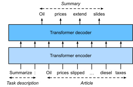
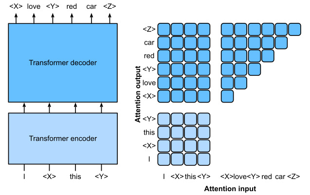
Fig. 11.9.4 explains fine-tuning T5 using text summarization as an example. In this downstream task, the task description tokens “Summarize”, “:” followed by the article tokens are input to the encoder.

그림 11.9.4는 텍스트 요약을 예로 들어 T5 미세 조정을 설명합니다. 이 다운스트림 작업에서 작업 설명 토큰 "Summarize", ":" 뒤에 기사 토큰이 인코더에 입력됩니다.

After fine-tuning, the 11-billion-parameter T5 (T5-11B) achieved state-of-the-art results on multiple encoding (e.g., classification) and generation (e.g., summarization) benchmarks. Since released, T5 has been extensively used in later research. For example, switch Transformers are designed based off T5 to activate a subset of the parameters for better computational efficiency (Fedus et al., 2022). In a text-to-image model called Imagen, text is input to a frozen T5 encoder (T5-XXL) with 4.6 billion parameters (Saharia et al., 2022). The photorealistic text-to-image examples in Fig. 11.9.5 suggest that the T5 encoder alone may effectively represent text even without fine-tuning.

미세 조정 후 110억 매개변수 T5(T5-11B)는 다중 인코딩(예: 분류) 및 생성(예: 요약) 벤치마크에서 최첨단 결과를 달성했습니다. 출시 이후 T5는 이후 연구에서 광범위하게 사용되었습니다. 예를 들어 스위치 트랜스포머는 더 나은 계산 효율성을 위해 매개변수의 하위 집합을 활성화하기 위해 T5를 기반으로 설계되었습니다(Fedus et al., 2022). Imagen이라는 텍스트-이미지 모델에서 텍스트는 46억 개의 매개변수가 있는 고정된 T5 인코더(T5-XXL)에 입력됩니다(Saharia et al., 2022). 그림 11.9.5의 사실적인 텍스트 대 이미지 예는 미세 조정 없이도 T5 인코더만으로도 텍스트를 효과적으로 표현할 수 있음을 시사합니다.

T5란?

T5(Tap-to-Transfer Transformer) is a versatile and powerful language model developed by Google Research in 2020. T5 is based on the transformer architecture, similar to BERT, and it takes the idea of transfer learning in natural language processing to a new level. The main innovation of T5 is its unified framework that can handle a wide range of NLP tasks using a single model.

T5(Tap-to-Transfer Transformer)은 2020년에 구글 리서치에서 개발한 다재다능한 언어 모델입니다. T5는 BERT와 마찬가지로 트랜스포머 아키텍처를 기반으로 하며, 자연어 처리의 전이 학습 아이디어를 새로운 수준으로 가져갑니다. T5의 주요 혁신은 하나의 모델로 다양한 NLP 작업을 처리할 수 있는 통합된 프레임워크입니다.

Here are some key points about T5:

다음은 T5에 관한 주요 사항입니다:

1. Transfer Learning for Various Tasks: T5 aims to simplify and unify the process of applying transformer models to various NLP tasks. Instead of developing separate models for different tasks like translation, text classification, question answering, and more, T5's single model can be fine-tuned for a wide array of tasks.
   
   다양한 작업에 대한 전이 학습: T5는 트랜스포머 모델을 다양한 NLP 작업에 적용하기 위한 과정을 단순화하고 통합하려는 목표를 가지고 있습니다. 번역, 텍스트 분류, 질의 응답 등 다양한 작업을 위해 별도의 모델을 개발하는 대신 T5의 단일 모델을 다양한 작업에 미세 조정할 수 있습니다.
   
   
2. Unified Text-to-Text Format: T5 approaches all NLP tasks as text-to-text tasks. This means that both input and output are treated as text sequences. For example, translation can be seen as translating an input sentence to an output sentence, text classification as classifying an input text into a category, and so on.
   
   통합된 텍스트-투-텍스트 형식: T5는 모든 NLP 작업을 텍스트-투-텍스트 작업으로 처리합니다. 이는 입력과 출력 모두를 텍스트 시퀀스로 처리하는 것을 의미합니다. 예를 들어, 번역은 입력 문장을 출력 문장으로 번역하는 작업으로 볼 수 있으며, 텍스트 분류는 입력 텍스트를 범주로 분류하는 작업과 같이 처리됩니다.
   
   
3. Pretraining and Fine-Tuning: T5 follows a two-step process: pretraining and fine-tuning. In the pretraining phase, the model is trained on a large corpus of text in an unsupervised manner, similar to how BERT is pretrained. In the fine-tuning phase, the pretrained model is adapted to specific tasks using labeled data.
   
   사전 훈련과 미세 조정: T5는 사전 훈련 및 미세 조정 두 단계의 프로세스를 따릅니다. 사전 훈련 단계에서 모델은 대규모 텍스트 말뭉치에서 무지성으로 훈련되며, BERT와 유사한 방식입니다. 미세 조정 단계에서는 사전 훈련된 모델이 레이블된 데이터를 사용하여 특정 작업에 적응되는 과정입니다.
   
   
4. Text Generation and Compression: T5 excels in both text generation and text compression tasks. It can generate coherent and contextually relevant text, making it suitable for tasks like language translation, summarization, and story generation. Additionally, it can compress longer texts into shorter, informative versions, which is valuable for tasks like data-to-text generation.
   
   텍스트 생성과 압축: T5는 텍스트 생성 및 텍스트 압축 작업 모두에서 뛰어난 성과를 보입니다. 일관되고 문맥에 맞는 텍스트를 생성할 수 있어 언어 번역, 요약, 이야기 생성과 같은 작업에 적합합니다. 더불어 긴 텍스트를 간결하면서도 정보를 잘 담은 형태로 압축하는 능력도 갖추고 있습니다. 이는 데이터를 텍스트로 변환하는 데이터-투-텍스트 생성 작업에 유용합니다.
   
   
5. Flexible Inputs and Outputs: T5 can accept various types of inputs and produce diverse outputs. For example, it can take prompts like "Translate the following English text to French: ..." and generate the translation. It can also be used for multiple-choice questions, summarization, and even image captioning by converting the task into text-to-text format.
   
   유연한 입력과 출력: T5는 다양한 유형의 입력을 받아들이고 다양한 출력을 생성할 수 있습니다. 예를 들어 "다음 영어 텍스트를 프랑스어로 번역하세요: ..."와 같은 프롬프트를 받아들이고 번역을 생성할 수 있습니다. 선택지 문제, 요약, 심지어 이미지 캡션 작업에도 텍스트-투-텍스트 형식으로 활용될 수 있습니다.
   
   
6. Large-Scale Model: Similar to other transformer models, T5 comes in different sizes, such as T5-small, T5-base, T5-large, and T5-3B, with increasing model parameters and capabilities.
   
   대규모 모델: 다른 트랜스포머 모델과 마찬가지로 T5는 T5-small, T5-base, T5-large, T5-3B 등 다양한 크기로 제공되며 모델 파라미터와 능력이 증가합니다.
   
   

T5's unified framework and its ability to handle a wide range of NLP tasks have made it a popular choice in the NLP community. It has achieved impressive results on various benchmarks and has contributed to advancing the field of natural language processing and understanding.

T5의 통합된 프레임워크와 다양한 NLP 작업을 처리하는 능력은 NLP 커뮤니티에서 인기를 얻었습니다. 다양한 벤치마크에서 놀라운 결과를 달성하며 자연어 처리와 이해 분야의 발전에 기여하였습니다.

11.9.3. Decoder-Only

We have reviewed encoder-only and encoder-decoder Transformers. Alternatively, decoder-only Transformers remove the entire encoder and the decoder sublayer with the encoder-decoder cross-attention from the original encoder-decoder architecture depicted in Fig. 11.7.1. Nowadays, decoder-only Transformers have been the de facto architecture in large-scale language modeling (Section 9.3), which leverages the world’s abundant unlabeled text corpora via self-supervised learning.

인코더 전용 및 인코더-디코더 transformer를 검토했습니다. 또는 디코더 전용 트랜스포머는 전체 인코더와 그림 11.7.1에 묘사된 원래 인코더-디코더 아키텍처에서 인코더-디코더 cross attention이 있는 디코더 하위 계층을 제거합니다. 오늘날 디코더 전용 트랜스포머는 대규모 언어 모델링(9.3절)에서 사실상의 아키텍처였으며, 이는 자기 지도 학습을 통해 전 세계의 풍부한 레이블 없는 텍스트 말뭉치를 활용합니다.

11.9.3.1. GPT and GPT-2

Using language modeling as the training objective, the GPT (generative pre-training) model chooses a Transformer decoder as its backbone (Radford et al., 2018).

학습 목표로 언어 모델링을 사용하는 GPT(Generative Pre-training) 모델은 Transformer 디코더를 백본으로 선택합니다(Radford et al., 2018).

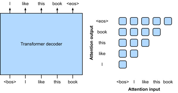
Following the autoregressive language model training as described in Section 9.3.3, Fig. 11.9.6 illustrates GPT pretraining with a Transformer encoder, where the target sequence is the input sequence shifted by one token. Note that the attention pattern in the Transformer decoder enforces that each token can only attend to its past tokens (future tokens cannot be attended to because they have not yet been chosen).

섹션 9.3.3에 설명된  autoregressive language model training에 이어 그림 11.9.6은 Transformer 인코더를 사용한 GPT 사전 교육을 보여줍니다. 여기서 대상 시퀀스는 하나의 토큰만큼 이동된 입력 시퀀스입니다. Transformer 디코더의 attention pattern은 각 토큰이 과거 토큰에만 attend할 수 있도록 합니다(미래의 토큰은 아직 선택되지 않았기 때문에 참석할 수 없음).

GPT has 100 million parameters and needs to be fine-tuned for individual downstream tasks. A much larger Transformer-decoder language model, GPT-2, was introduced one year later (Radford et al., 2019). Compared with the original Transformer decoder in GPT, pre-normalization (discussed in Section 11.8.3) and improved initialization and weight-scaling were adopted in GPT-2. Pretrained on 40 GB of text, the 1.5-billion-parameter GPT-2 obtained the state-of-the-art results on language modeling benchmarks and promising results on multiple other tasks without updating the parameters or architecture.

GPT에는 1억 개의 매개변수가 있으며 개별 다운스트림 작업에 맞게 미세 조정해야 합니다. 훨씬 더 큰 Transformer-decoder 언어 모델인 GPT-2가 1년 후에 도입되었습니다(Radford et al., 2019). GPT의 원래 Transformer 디코더와 비교하여 사전 정규화(11.8.3절에서 설명)와 향상된 초기화 및 가중치 스케일링이 GPT-2에 채택되었습니다. 40GB의 텍스트로 사전 훈련된 15억 개의 매개변수 GPT-2는 언어 모델링 벤치마크에서 최신 결과를 얻었고 매개변수나 아키텍처를 업데이트하지 않고도 여러 다른 작업에서 유망한 결과를 얻었습니다.

11.9.3.2. GPT-3

GPT-2 demonstrated potential of using the same language model for multiple tasks without updating the model. This is more computationally efficient than fine-tuning, which requires model updates via gradient computation.

GPT-2는 모델을 업데이트하지 않고 여러 작업에 동일한 언어 모델을 사용할 수 있는 가능성을 보여주었습니다. 이것은 그래디언트 계산을 통해 모델을 업데이트해야 하는 미세 조정보다 계산적으로 더 효율적입니다.

Before explaining the more computationally efficient use of language models without parameter update, recall Section 9.5 that a language model can be trained to generate a text sequence conditional on some prefix text sequence. Thus, a pretrained language model may generate the task output as a sequence without parameter update, conditional on an input sequence with the task description, task-specific input-output examples, and a prompt (task input). This learning paradigm is called in-context learning (Brown et al., 2020), which can be further categorized into zero-shot, one-shot, and few-shot, when there is no, one, and a few task-specific input-output examples, respectively (Fig. 11.9.7).

매개 변수 업데이트 없이 언어 모델을 보다 계산적으로 효율적으로 사용하는 방법을 설명하기 전에 일부 접두사 텍스트 시퀀스에 조건부 텍스트 시퀀스를 생성하도록 언어 모델을 훈련할 수 있다는 섹션 9.5를 상기하십시오. 따라서 미리 훈련된 언어 모델은 작업 설명, 작업별 입력-출력 예제 및 프롬프트(작업 입력)가 있는 입력 시퀀스에 따라 매개 변수 업데이트 없이 시퀀스로 작업 출력을 생성할 수 있습니다. 이러한 학습 패러다임을 in-context learning(Brown et al., 2020)이라고 하며, 더 나아가 제로샷(zero-shot), 원샷(one-shot), 퓨어샷(female-shot)으로 분류할 수 있다. 각각 입력-출력 예(그림 11.9.7).

in-context learning이란?

'In-context learning'은 주어진 문맥(context) 내에서 학습하는 개념을 나타냅니다. 이것은 기계 학습 또는 딥 러닝 모델이 주어진 데이터 포인트를 주변 문맥과 관련하여 학습하고 예측하는 것을 의미합니다.

예를 들어, 자연어 처리(NLP)에서 특정 단어의 의미를 이해하려면 해당 단어의 주변 문맥을 고려해야 합니다. 이를 위해 주어진 단어 주변의 단어들을 입력으로 사용하여 모델을 학습하고, 주변 문맥을 통해 해당 단어의 의미를 파악하려는 것이 'in-context learning'입니다.

'In-context learning'은 문제를 더 정확하게 이해하고 예측하기 위해 문맥 정보를 활용하는 중요한 방법 중 하나입니다. 이는 자연어 처리, 컴퓨터 비전, 음성 처리 등 다양한 분야에서 활용되며, 모델의 성능을 향상시키는 데 도움이 됩니다.

zero-shot, one-shot, few shot이란?

'Zero-shot', 'one-shot', 그리고 'few-shot'은 머신 러닝 및 딥 러닝에서 사용되는 학습 접근 방식을 나타내는 용어입니다.

1. Zero-shot Learning (제로샷 학습): 제로샷 학습은 학습 데이터 없이 새로운 클래스 또는 작업에 대한 학습을 시도하는 접근 방식입니다. 모델은 이미 학습된 정보를 기반으로 새로운 데이터에 대한 예측을 수행합니다. 이를 위해 추가 정보나 외부 지식을 활용하는 경우가 많습니다.
   
   
2. One-shot Learning (원샷 학습): 원샷 학습은 매우 작은 수의 학습 데이터만을 이용하여 새로운 클래스 또는 작업에 대한 학습을 시도하는 접근 방식입니다. 예를 들어, 하나의 학습 샘플만 사용하여 클래스를 구분하는 작업을 수행하는 것을 말합니다.
   
   
3. Few-shot Learning (퓨샷 학습): 퓨샷 학습은 원샷 학습과 비슷하지만, 더 큰 데이터 셋에서 몇 개의 학습 샘플을 사용하여 새로운 클래스나 작업에 대한 학습을 시도하는 접근 방식입니다. 보통 5개 이하의 학습 샘플을 사용하는 경우를 말합니다.
   
   

이러한 접근 방식들은 데이터가 부족한 상황에서 새로운 클래스나 작업에 대한 모델을 구축할 때 유용하게 활용될 수 있습니다.

http://cartinoe5930.tistory.com/54

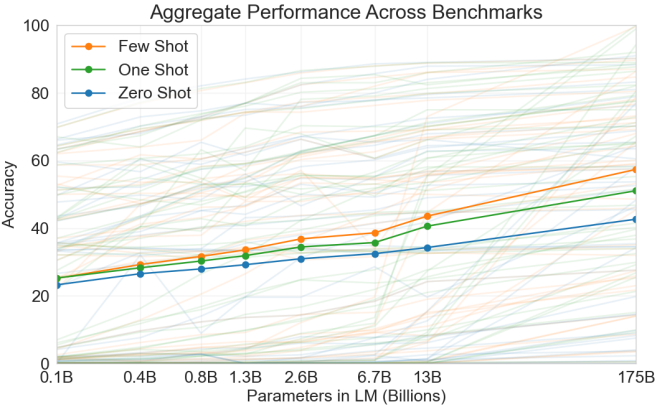
These three settings were tested in GPT-3 (Brown et al., 2020), whose largest version uses data and model size about two orders of magnitude larger than those in GPT-2. GPT-3 uses the same Transformer decoder architecture in its direct predecessor GPT-2 except that attention patterns (right of Fig. 11.9.6) are sparser at alternating layers. Pretrained with 300 billion tokens, GPT-3 performs better with larger model size, where few-shot performance increases most rapidly (Fig. 11.9.8).

이 세 가지 설정은 GPT-3(Brown et al., 2020)에서 테스트되었으며, 가장 큰 버전은 GPT-2보다 약 2배 더 큰 데이터와 모델 크기를 사용합니다. GPT-3는 어텐션 패턴(그림 11.9.6의 오른쪽)이 교대 레이어에서 희박하다는 점을 제외하면 이전 GPT-2와 동일한 트랜스포머 디코더 아키텍처를 사용합니다. 3000억 개의 토큰으로 사전 훈련된 GPT-3는 더 큰 모델 크기에서 더 나은 성능을 발휘하며 여기서 퓨샷 성능이 가장 빠르게 증가합니다(그림 11.9.8).

Large language models offer an exciting prospect of formulating text input to induce models to perform desired tasks via in-context learning, which is also known as prompting. For example, chain-of-thought prompting (Wei et al., 2022), an in-context learning method with few-shot “question, intermediate reasoning steps, answer” demonstrations, elicits the complex reasoning capabilities of large language models to solve mathematical, commonsense, and symbolic reasoning tasks. Sampling multiple reasoning paths (Wang et al., 2023), diversifying few-shot demonstrations (Zhang et al., 2023), and reducing complex problems to sub-problems (Zhou et al., 2023) can all improve the reasoning accuracy. In fact, with simple prompts like “Let’s think step by step” just before each answer, large language models can even perform zero-shot chain-of-thought reasoning with decent accuracy (Kojima et al., 2022). Even for multimodal inputs consisting of both text and images, language models can perform multimodal chain-of-thought reasoning with further improved accuracy than using text input only (Zhang et al., 2023).

대규모 언어 모델은 프롬프트라고도 하는 in-context learning을 통해 모델이 원하는 작업을 수행하도록 유도하기 위해 텍스트 입력을 공식화하는 흥미로운 전망을 제공합니다. 예를 들어, 몇 번의 "질문, 중간 추론 단계, 답변" 데모가 포함된 상황 내 학습 방법인 chain-of-thought prompting(Wei et al., 2022)는 문제를 해결하기 위해 대규모 언어 모델의 복잡한 추론 기능을 이끌어냅니다. 수학, 상식 및 상징적 추론 작업. 다중 추론 경로 샘플링(Wang et al., 2023), 소수 샷 시연 다양화(Zhang et al., 2023), 복잡한 문제를 하위 문제로 줄이는 것(Zhou et al., 2023) 모두 추론 정확도를 향상시킬 수 있습니다. 사실, 각 답변 직전에 "차근차근 생각해 봅시다"와 같은 간단한 프롬프트를 통해 대규모 언어 모델은 적절한 정확도로 제로샷 연쇄 사고 추론을 수행할 수도 있습니다(Kojima et al., 2022). 텍스트와 이미지로 구성된 다중 모드 입력의 경우에도 언어 모델은 텍스트 입력만 사용하는 것보다 더 향상된 정확도로 다중 모드 사고 연쇄 추론을 수행할 수 있습니다(Zhang et al., 2023).

11.9.4. Scalability

Fig. 11.9.8 empirically demonstrates scalability of Transformers in the GPT-3 language model. For language modeling, more comprehensive empirical studies on the scalability of Transformers have led researchers to see promise in training larger Transformers with more data and compute (Kaplan et al., 2020).

그림 11.9.8은 GPT-3 언어 모델에서 Transformers의 확장성을 실증적으로 보여준다. 언어 모델링의 경우 Transformers의 확장성에 대한 보다 포괄적인 경험적 연구를 통해 연구자들은 더 많은 데이터와 컴퓨팅으로 더 큰 Transformers를 교육할 가능성을 확인했습니다(Kaplan et al., 2020).

As shown in Fig. 11.9.9, power-law scaling can be observed in the performance with respect to the model size (number of parameters, excluding embedding layers), dataset size (number of training tokens), and amount of training compute (PetaFLOP/s-days, excluding embedding layers). In general, increasing all these three factors in tandem leads to better performance. However, how to increase them in tandem still remains a matter of debate (Hoffmann et al., 2022).

그림 11.9.9에서와 같이 Model size (number of parameters, excluding embedding layers), data size (number of training tokens) 그리고 amount of training compute (PetaFLOP/s-days, excluding embedding layers) 가 늘어날 수록 성능이 좋아진다. ==> power-law scaling을 볼 수 있다. 그러나 그것들을 동시에 증가시키는 방법은 여전히 논쟁의 문제로 남아 있습니다(Hoffmann et al., 2022).

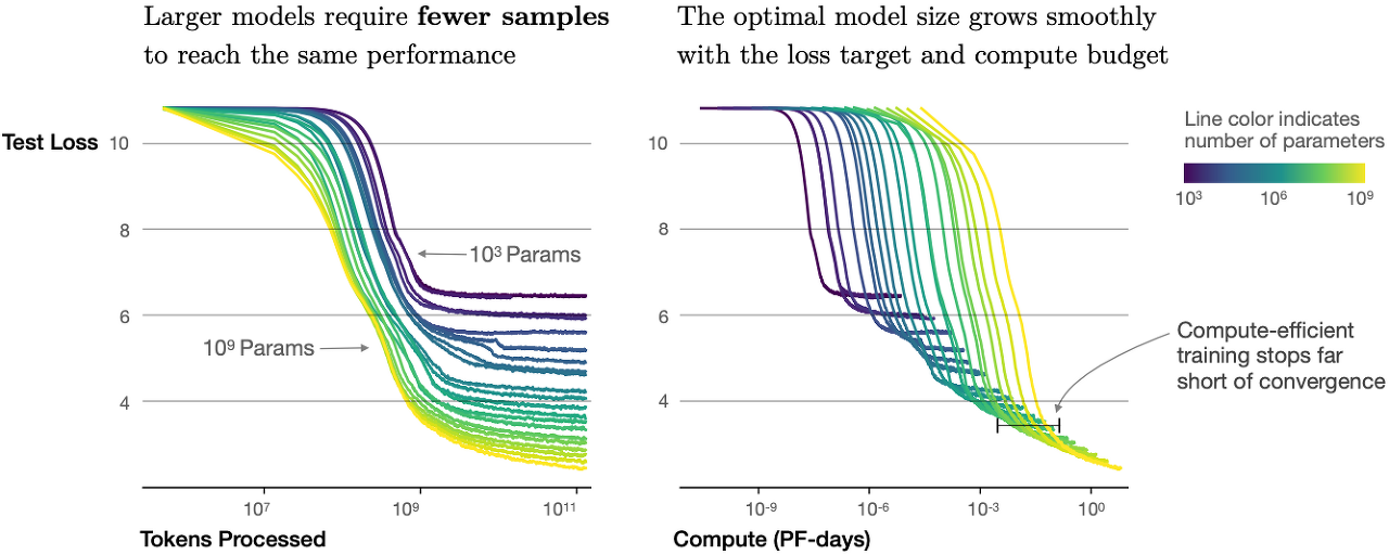
Besides increased performance, large models also enjoy better sample efficiency than small models. Fig. 11.9.10 shows that large models need fewer training samples (tokens processed) to perform at the same level achieved by small models, and performance is scaled smoothly with compute.

향상된 성능 외에도 대형 모델은 소형 모델보다 샘플 효율성이 더 좋습니다. 그림 11.9.10은 작은 모델이 달성한 것과 동일한 수준에서 수행하기 위해 더 적은 수의 교육 샘플(처리된 토큰)이 필요한 큰 모델을 보여 주며 성능은 컴퓨팅을 통해 원활하게 확장됩니다.

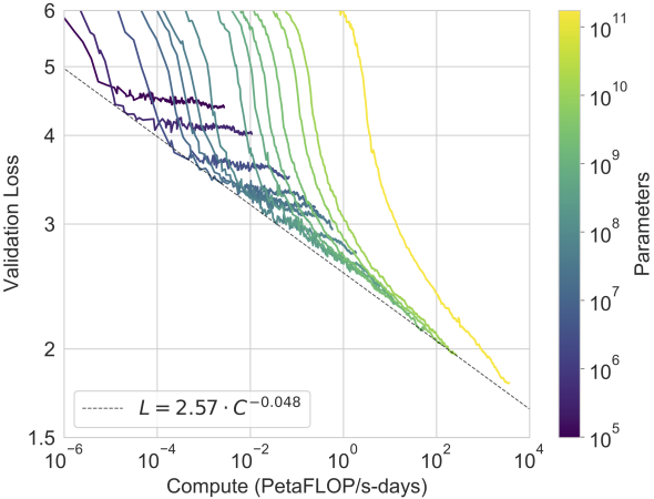
The empirical scaling behaviors in Kaplan et al. (2020) have been tested in subsequent large Transformer models. For example, GPT-3 supported this hypothesis with two more orders of magnitude in Fig. 11.9.11.

Kaplan et al.의 경험적 스케일링 동작. (2020) 이후의 대형 Transformer 모델에서 테스트되었습니다. 예를 들어, GPT-3는 그림 11.9.11에서 두 자릿수 이상의 크기로 이 가설을 뒷받침했습니다.

The scalability of Transformers in the GPT series has inspired subsequent Transformer language models. While the Transformer decoder in GPT-3 was largely followed in OPT (Open Pretrained Transformers) (Zhang et al., 2022) using only 1/7th the carbon footprint of the former, the GPT-2 Transformer decoder was used in training the 530-billion-parameter Megatron-Turing NLG (Smith et al., 2022) with 270 billion training tokens. Following the GPT-2 design, the 280-billion-parameter Gopher (Rae et al., 2021) pretrained with 300 billion tokens achieved state-of-the-art performance across the majority on about 150 diverse tasks. Inheriting the same architecture and using the same compute budget of Gopher, Chinchilla (Hoffmann et al., 2022) is a substantially smaller (70 billion parameters) model that trains much longer (1.4 trillion training tokens), outperforming Gopher on many tasks. To continue the scaling line of language modeling, PaLM (Pathway Language Model) (Chowdhery et al., 2022), a 540-billion-parameter Transformer decoder with modified designs pretrained on 780 billion tokens, outperformed average human performance on the BIG-Bench benchmark (Srivastava et al., 2022). Further training PaLM on 38.5 billion tokens containing scientific and mathematical content results in Minerva (Lewkowycz et al., 2022), a large language model that can answer nearly a third of undergraduate-level problems that require quantitative reasoning, such as in physics, chemistry, biology, and economics.

GPT 시리즈의 트랜스포머 확장성은 후속 트랜스포머 언어 모델에 영감을 주었습니다. GPT-3의 Transformer 디코더는 OPT(Open Pretrained Transformers)(Zhang et al., 2022)에서 전자의 탄소 발자국의 1/7만 사용하여 주로 따랐지만 GPT-2 Transformer 디코더는 530을 교육하는 데 사용되었습니다. - 2700억 개의 훈련 토큰이 있는 10억 개의 매개변수 Megatron-Turing NLG(Smith et al., 2022). GPT-2 설계에 따라 3000억 개의 토큰으로 사전 훈련된 2800억 개의 매개변수 Gopher(Rae et al., 2021)는 약 150개의 다양한 작업에서 대다수에 걸쳐 최첨단 성능을 달성했습니다. 동일한 아키텍처를 상속하고 Gopher의 동일한 컴퓨팅 예산을 사용하는 Chinchilla(Hoffmann et al., 2022)는 훨씬 더 오래(1조 4천억 개의 훈련 토큰) 훈련하는 상당히 작은(700억 매개변수) 모델로 많은 작업에서 Gopher를 능가합니다. 언어 모델링의 스케일링 라인을 계속하기 위해, 7,800억 개의 토큰으로 사전 훈련된 수정된 설계가 있는 5,400억 개의 매개변수 Transformer 디코더인 PaLM(Pathway Language Model)(Chowdhery et al., 2022)은 BIG-Bench에서 평균적인 인간 성능을 능가했습니다. 벤치마크(Srivastava et al., 2022). 과학 및 수학적 콘텐츠가 포함된 385억 개의 토큰에 대해 PaLM을 추가로 교육하면 물리학, 화학과 같이 정량적 추론이 필요한 학부 수준 문제의 거의 1/3에 답할 수 있는 대규모 언어 모델인 Minerva(Lewkowycz et al., 2022)가 생성됩니다. , 생물학 및 경제학.

Wei et al. (2022) discussed emergent abilities of large language models that are only present in larger models, but not present in smaller models. However, simply increasing model size does not inherently make models follow human instructions better. Following InstructGPT that aligns language models with human intent via fine-tuning (Ouyang et al., 2022), ChatGPT is able to follow instructions, such as code debugging and note drafting, from its conversations with humans.

Weiet al. (2022)는 더 큰 모델에만 존재하고 더 작은 모델에는 존재하지 않는 대규모 언어 모델의 창발적 능력에 대해 논의했습니다. 그러나 단순히 모델 크기를 늘리는 것이 본질적으로 모델이 사람의 지시를 더 잘 따르도록 만들지는 않습니다. 미세 조정을 통해 언어 모델을 인간의 의도에 맞추는 InstructGPT(Ouyang et al., 2022)에 이어 ChatGPT는 인간과의 대화에서 코드 디버깅 및 메모 작성과 같은 지침을 따를 수 있습니다.

GPT, GPT2, GPT3에 대하여.

GPT (Generative Pre-trained Transformer) series refers to a sequence of language models developed by OpenAI, each building upon the success and innovations of the previous version. These models are designed based on the Transformer architecture, which has proven to be highly effective for a wide range of natural language processing tasks. Here's an overview of each model:

GPT(Generative Pre-trained Transformer) 시리즈는 OpenAI에서 개발한 언어 모델 시퀀스로, 각 버전이 이전 버전의 성과와 혁신을 기반으로 발전되었습니다. 이 모델들은 Transformer 아키텍처를 기반으로 설계되어 다양한 자연어 처리 작업에 높은 효율성을 보입니다. 각 모델에 대한 개요는 아래와 같습니다:

1. GPT-1 (Generative Pre-trained Transformer 1): GPT-1 was the first model in the series. It introduced the concept of pre-training a large neural network on a massive amount of text data and then fine-tuning it on specific downstream tasks. It used a decoder-only Transformer architecture and demonstrated impressive performance on various language tasks. However, it was limited by its relatively smaller size compared to later versions.
   
   GPT-1 (Generative Pre-trained Transformer 1): GPT-1은 시리즈에서 처음 나온 모델입니다. 이 모델은 대량의 텍스트 데이터에서 큰 신경망을 사전 훈련하고 특정 하위 작업에 대해 세밀하게 튜닝하는 개념을 소개했습니다. 디코더만을 사용하는 Transformer 아키텍처를 사용하였으며, 다양한 언어 작업에서 인상적인 성능을 보였습니다. 하지만 이후 버전들과 비교하여 크기가 상대적으로 작아 제한된 성능을 보였습니다.
   
   
2. GPT-2 (Generative Pre-trained Transformer 2): GPT-2 was a significant leap forward in terms of size and capabilities. It gained widespread attention for its large number of parameters (up to 1.5 billion) and its ability to generate coherent and contextually relevant text. GPT-2 was so powerful that OpenAI initially chose not to release its largest versions due to concerns about potential misuse for generating fake news or deceptive content. GPT-2 showed remarkable performance across a wide range of tasks and achieved state-of-the-art results on various benchmarks.
   
   GPT-2 (Generative Pre-trained Transformer 2): GPT-2는 크기와 성능 면에서 큰 도약을 이루었습니다. 15억 개의 파라미터를 가진 대규모 모델로, 연관성 있는 문장을 생성하는 능력으로 널리 주목받았습니다. GPT-2는 파라미터의 많은 양과 함께 크고 복잡한 텍스트를 생성할 수 있는 능력으로 유명해졌습니다. GPT-2는 다양한 작업에서 높은 성능을 보여주며 다양한 벤치마크에서 최고 수준의 결과를 달성했습니다.
   
   
3. GPT-3 (Generative Pre-trained Transformer 3): GPT-3 marked another substantial advancement in the series. With a staggering 175 billion parameters, GPT-3 is one of the largest language models ever created. It demonstrated the ability to generate highly coherent and contextually relevant text across a wide variety of prompts. What makes GPT-3 particularly remarkable is its "few-shot" or "zero-shot" learning capabilities. It can perform tasks with minimal examples or even no explicit training, as long as the task is described in the prompt.
4. GPT-3's versatility has allowed it to excel in tasks ranging from translation and summarization to question answering and code generation. However, GPT-3 also raised concerns about biases present in its training data and the ethical implications of such powerful language models.

GPT-3 (Generative Pre-trained Transformer 3): GPT-3는 시리즈의 또 다른 큰 발전을 이루었습니다. 1750억 개의 파라미터를 가지며, 이는 역사적으로 가장 큰 언어 모델 중 하나입니다. GPT-3는 문맥상 관련성이 높은 텍스트를 다양한 프롬프트에 대해 생성할 수 있는 능력을 보였습니다. 특히 GPT-3의 놀라운 점은 "few-shot" 또는 "zero-shot" 학습 능력입니다. 몇 개의 예시나 아예 훈련이 없더라도 프롬프트에 명시된 작업을 수행할 수 있습니다.

GPT-3의 다재다능함은 번역, 요약, 질문 답변, 코드 생성과 같은 다양한 작업에서 뛰어난 성과를 거두게 했습니다. 하지만 GPT-3는 훈련 데이터의 편향성과 같은 문제, 그리고 이러한 강력한 언어 모델의 윤리적인 측면에 대한 우려를 불러일으켰습니다.

All of these models, GPT-1, GPT-2, and GPT-3, are part of the broader trend of using large-scale pre-training followed by fine-tuning for specific tasks. They have contributed significantly to advancing the field of natural language processing and understanding.

GPT-1, GPT-2 및 GPT-3는 모두 대량 사전 훈련 후 특정 작업에 대한 세부 튜닝을 통한 넓은 범위의 프레임워크를 대표합니다. 이들은 자연어 처리 및 이해 분야를 크게 발전시키는 데 기여한 중요한 모델 시리즈입니다.

11.9.5. Summary and Discussion

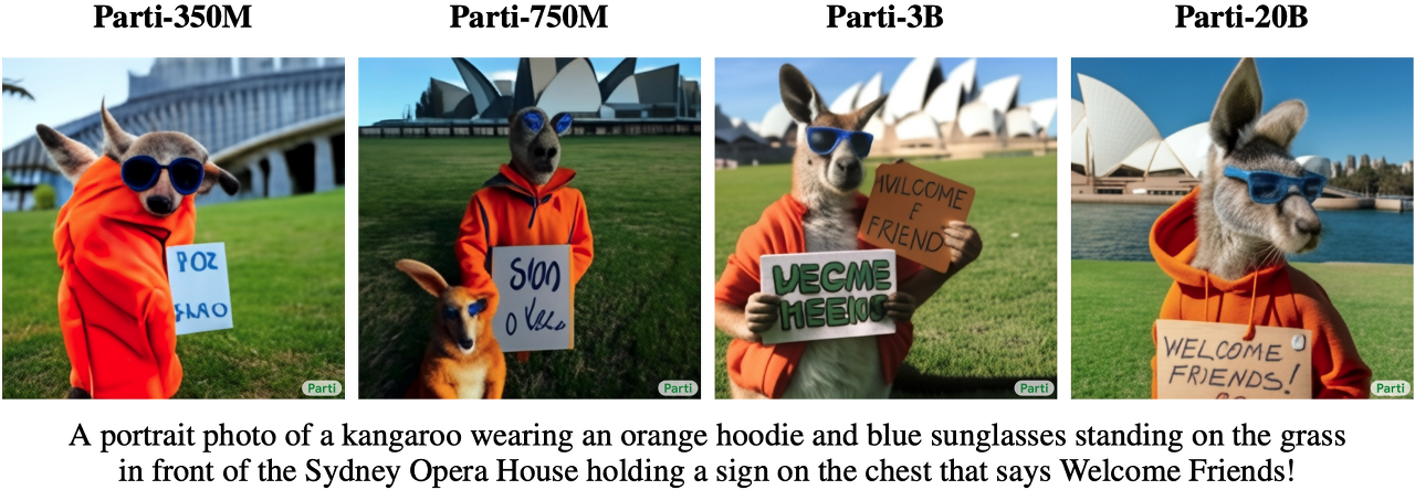
Transformers have been pretrained as encoder-only (e.g., BERT), encoder-decoder (e.g., T5), and decoder-only (e.g., GPT series). Pretrained models may be adapted to perform different tasks with model update (e.g., fine tuning) or not (e.g., few shot). Scalability of Transformers suggests that better performance benefits from larger models, more training data, and more training compute. Since Transformers were first designed and pretrained for text data, this section leans slightly towards natural language processing. Nonetheless, those models discussed above can be often found in more recent models across multiple modalities. For example, (i) Chinchilla (Hoffmann et al., 2022) was further extended to Flamingo (Alayrac et al., 2022), a visual language model for few-shot learning; (ii) GPT-2 (Radford et al., 2019) and the vision Transformer encode text and images in CLIP (Contrastive Language-Image Pre-training) (Radford et al., 2021), whose image and text embeddings were later adopted in the DALL-E 2 text-to-image system (Ramesh et al., 2022). Although there has been no systematic studies on Transformer scalability in multi-modal pretraining yet, a recent all-Transformer text-to-image model, Parti (Yu et al., 2022), shows potential of scalability across modalities: a larger Parti is more capable of high-fidelity image generation and content-rich text understanding (Fig. 11.9.12).

트랜스포머는 인코더 전용(예: BERT), 인코더-디코더(예: T5) 및 디코더 전용(예: GPT 시리즈)으로 사전 훈련되었습니다. 사전 훈련된 모델은 모델 업데이트(예: 미세 조정) 또는 그렇지 않은(예: 소수 샷) 다른 작업을 수행하도록 조정될 수 있습니다. Transformers의 확장성은 더 큰 모델, 더 많은 교육 데이터 및 더 많은 교육 컴퓨팅에서 더 나은 성능 이점을 제공합니다. 트랜스포머는 처음에 텍스트 데이터용으로 설계되고 사전 훈련되었기 때문에 이 섹션은 자연어 처리에 약간 기울어져 있습니다. 그럼에도 불구하고 위에서 논의한 모델은 종종 여러 양식에 걸친 최신 모델에서 찾을 수 있습니다. 예를 들어, (i) 친칠라(Hoffmann et al., 2022)는 퓨어샷 학습을 위한 시각적 언어 모델인 Flamingo(Alayrac et al., 2022)로 더욱 확장되었습니다. (ii) GPT-2(Radford et al., 2019) 및 비전 트랜스포머는 CLIP(Contrastive Language-Image Pre-training)(Radford et al., 2021)에서 텍스트와 이미지를 인코딩하며, 이미지 및 텍스트 임베딩은 나중에 채택되었습니다. DALL-E 2 텍스트-이미지 시스템에서(Ramesh et al., 2022). 다중 모달 사전 훈련에서 Transformer 확장성에 대한 체계적인 연구는 아직 없지만 최근의 모든 변환기 텍스트-이미지 모델인 Parti(Yu et al., 2022)는 양식에 걸친 확장 가능성을 보여줍니다. 더 큰 Parti는 고화질 이미지 생성 및 내용이 풍부한 텍스트 이해가 더 가능합니다(그림 11.9.12).

11.9.6. Exercises

1. Is it possible to fine tune T5 using a minibatch consisting of different tasks? Why or why not? How about for GPT-2?
2. Given a powerful language model, what applications can you think of?
3. Say that you are asked to fine tune a language model to perform text classification by adding additional layers. Where will you add them? Why?
4. Consider sequence to sequence problems (e.g., machine translation) where the input sequence is always available throughout the target sequence prediction. What could be limitations of modeling with decoder-only Transformers? Why?

https://d2l.ai/chapter_attention-mechanisms-and-transformers/vision-transformer.html

The Transformer architecture was initially proposed for sequence to sequence learning, with a focus on machine translation. Subsequently, Transformers emerged as the model of choice in various natural language processing tasks (Brown et al., 2020, Devlin et al., 2018, Radford et al., 2018, Radford et al., 2019, Raffel et al., 2020). However, in the field of computer vision the dominant architecture has remained the CNN (Section 8). Naturally, researchers started to wonder if it might be possible to do better by adapting Transformer models to image data. This question sparked immense interest in the computer vision community. Recently, Ramachandran et al. (2019) proposed a scheme for replacing convolution with self-attention. However, its use of specialized patterns in attention makes it hard to scale up models on hardware accelerators. Then, Cordonnier et al. (2020) theoretically proved that self-attention can learn to behave similarly to convolution. Empirically, 2×2 patches were taken from images as inputs, but the small patch size makes the model only applicable to image data with low resolutions.

Transformer 아키텍처는 처음에 기계 번역에 중점을 둔 sequence to sequence learning을 위해 제안되었습니다. 이후 Transformers는 다양한 자연어 처리 작업에서 선택 모델로 등장했습니다(Brown et al., 2020, Devlin et al., 2018, Radford et al., 2018, Radford et al., 2019, Raffel et al., 2020). ). 그러나 컴퓨터 비전 분야에서 지배적인 아키텍처는 CNN으로 남아 있습니다(섹션 8). 당연히 연구자들은 Transformer 모델을 이미지 데이터에 적용하여 더 잘할 수 있을지 궁금해하기 시작했습니다. 이 질문은 컴퓨터 비전 커뮤니티에서 엄청난 관심을 불러일으켰습니다. 최근 Ramachandran et al. (2019)는 컨볼루션을 self-attention으로 대체하는 방식을 제안했습니다. 그러나 어텐션에 특화된 패턴을 사용하면 hardware accelerators에서 모델을 확장하기가 어렵습니다. ??? 그런 다음 Cordonnier et al. (2020)은 self-attention이 convolution과 유사하게 동작하도록 학습할 수 있음을 이론적으로 증명했습니다. 경험적으로 이미지에서 2×2 패치를 입력으로 가져왔지만 패치 크기가 작기 때문에 모델은 해상도가 낮은 이미지 데이터에만 적용할 수 있습니다.

Without specific constraints on patch size, vision Transformers (ViTs) extract patches from images and feed them into a Transformer encoder to obtain a global representation, which will finally be transformed for classification (Dosovitskiy et al., 2021). Notably, Transformers show better scalability than CNNs: when training larger models on larger datasets, vision Transformers outperform ResNets by a significant margin. Similar to the landscape of network architecture design in natural language processing, Transformers also became a game-changer in computer vision.

패치 크기에 대한 특정 제약 없이 vision Transformers (ViTs)는 이미지에서 패치를 추출하고 트랜스포머 인코더에 공급하여 최종적으로 분류를 위해 변환될 글로벌 representation을 얻습니다(Dosovitskiy et al., 2021). 특히 트랜스포머는 CNN보다 더 나은 확장성을 보여줍니다. 더 큰 데이터 세트에서 더 큰 모델을 교육할 때 비전 트랜스포머는 ResNets보다 훨씬 뛰어난 성능을 보입니다. 자연어 처리의 네트워크 아키텍처 설계 환경과 유사하게 Transformers도 컴퓨터 비전의 게임 체인저가 되었습니다.

import torch
from torch import nn
from d2l import torch as d2l

11.8.1. Model

Fig. 11.8.1 depicts the model architecture of vision Transformers. This architecture consists of a stem that patchifies images, a body based on the multi-layer Transformer encoder, and a head that transforms the global representation into the output label.

그림 11.8.1은 비전 트랜스포머의 모델 아키텍처를 보여줍니다. 이 아키텍처는 이미지를 패치하는 stem , multi-layer Transformer encoder를 기반으로 하는 body, global representation을 output label로 변환하는 head 로 구성됩니다.

Consider an input image with height ℎ, width h, and w channels. Specifying the patch height and width both as p, the image is split into a sequence of m=ℎw/p^2 patches, where each patch is flattened to a vector of length cp^2. In this way, image patches can be treated similarly to tokens in text sequences by Transformer encoders. A special “<cls>” (class) token and the m flattened image patches are linearly projected into a sequence of m+1 vectors, summed with learnable positional embeddings. The multi-layer Transformer encoder transforms m+1 input vectors into the same amount of output vector representations of the same length. It works exactly the same way as the original Transformer encoder in Fig. 11.7.1, only differing in the position of normalization. Since the “<cls>” token attends to all the image patches via self-attention (see Fig. 11.6.1), its representation from the Transformer encoder output will be further transformed into the output label.

높이 ℎ, 너비 h 및 w 채널이 있는 입력 이미지를 고려하십시오. 패치 높이와 너비를 모두 p로 지정하면 이미지가 m=ℎw/p^2 패치 시퀀스로 분할되며 각 패치는 길이 cp^2의 벡터로 병합됩니다. 이러한 방식으로 이미지 패치는 Transformer 인코더에 의해 텍스트 시퀀스의 토큰과 유사하게 처리될 수 있습니다. 특수 "<cls>"(클래스) 토큰과 m개의 평면화된 이미지 패치는 학습 가능한 위치 임베딩으로 합산된 일련의 m+1 벡터로 선형 투영됩니다. 다층 트랜스포머 인코더는 m+1개의 입력 벡터를 같은 길이의 같은 양의 출력 벡터 표현representations 으로 변환합니다. 정규화 위치만 다를 뿐 그림 11.7.1의 원래 Transformer 인코더와 정확히 동일한 방식으로 작동합니다. "<cls>" 토큰은 self-attention(그림 11.6.1 참조)을 통해 모든 이미지 패치에 attends 하므로 Transformer 인코더 출력의 representation 은 출력 레이블로 추가 변환됩니다.

Tip. Deep Learning에서 Feature와 Representation 이란?

In the context of deep learning, the terms "feature" and "representation" are closely related concepts, but they have slightly different meanings.

딥 러닝의 맥락에서 "특징"과 "표현"이라는 용어는 밀접한 관련이 있는 개념이지만, 약간의 차이가 있습니다.

Feature: A feature refers to a specific property, characteristic, or aspect of the input data that is relevant for solving a particular task. Features are often extracted or selected from raw data to provide meaningful and informative input to a machine learning or deep learning model. Features can be thought of as the input variables or attributes that the model uses to make predictions or decisions. In deep learning, features can be learned automatically through the layers of a neural network.

특징은 특정 작업을 해결하는 데 관련성 있는 입력 데이터의 특정 속성, 특성 또는 측면을 나타냅니다. 특징은 종종 원시 데이터에서 추출되거나 선택되어 기계 학습 또는 딥 러닝 모델에 의해 의미 있는 정보를 제공하는 입력을 제공합니다. 특징은 모델이 예측하거나 결정하는 데 사용하는 입력 변수 또는 속성으로 생각할 수 있습니다. 딥 러닝에서는 특징은 신경망의 레이어를 통해 자동으로 학습될 수 있습니다.

For example, in image recognition, features could be the presence of edges, corners, textures, or specific patterns within an image. In natural language processing, features could include the frequency of certain words or phrases in a text document.

예를 들어 이미지 인식에서 특징은 이미지 내의 가장자리, 모서리, 질감 또는 특정 패턴의 존재와 관련이 있을 수 있습니다. 자연어 처리에서 특징은 텍스트 문서에서 특정 단어 또는 구문의 빈도와 관련할 수 있습니다.

Representation: Representation, on the other hand, is a broader term that encompasses the entire encoding of the input data in a format that can be processed by a machine learning model. Representation refers to how the input data is transformed and structured to be compatible with the model's architecture and learning process. It includes both the extracted features and any additional transformation that might be applied to the data.

한편, 표현은 입력 데이터를 모델이 처리할 수 있는 형식으로 전체적으로 인코딩하는 것을 나타냅니다. 표현은 입력 데이터가 모델의 아키텍처 및 학습 과정과 호환되도록 변환되고 구조화된 방식을 포함합니다. 이것은 추출된 특징 및 데이터에 적용된 추가 변환을 모두 포함합니다.

In deep learning, representations are often learned hierarchically through the layers of neural networks. Each layer extracts increasingly abstract and complex features from the previous layer's representation, gradually building a more informative and discriminating representation of the input data. The final learned representation is then used for making predictions or classifications.

딥 러닝에서 표현은 종종 신경망의 레이어를 통해 계층적으로 학습됩니다. 각 레이어는 이전 레이어의 표현에서 점점 추상적이고 복잡한 특징을 추출하여 입력 데이터의 보다 의미 있는 표현을 점진적으로 구축합니다. 최종 학습된 표현은 예측이나 분류를 위해 사용됩니다.

In summary, features are specific characteristics of the data that are relevant to a task, while representation is the overall encoding of the data that captures relevant information and is used by the model for learning and making predictions.

요약하자면, 특징은 작업에 관련된 데이터의 특정 특성이며, 표현은 입력 데이터의 전체적인 인코딩으로써 관련 정보를 포착하고 모델의 학습과 예측에 사용되는 것입니다.

CNN에서 Channel 이란?

In Convolutional Neural Networks (CNNs), a "channel" refers to one of the dimensions of the input data and the corresponding learned filters. In the context of images, which are commonly used with CNNs, the term "channel" typically refers to the color channels or color planes of an image. Each channel represents a specific color component: red, green, and blue (RGB), in the case of a standard color image.

합성곱 신경망(CNN)에서 "채널"은 입력 데이터와 해당하는 학습된 필터의 차원 중 하나를 가리킵니다. 이미지와 함께 주로 사용되는 CNN의 맥락에서 "채널"이라는 용어는 일반적으로 이미지의 색상 채널 또는 컬러 플레인을 의미합니다. 각 채널은 특정한 색상 구성요소를 나타냅니다. 표준 컬러 이미지의 경우 빨강, 초록 및 파랑(RGB)에 해당하는 채널이 있습니다.

For example, in an RGB image, there are three color channels: one for red, one for green, and one for blue. Each channel contains pixel values that represent the intensity of the corresponding color component for each pixel in the image. These channels are stacked together to create the full color image.

예를 들어 RGB 이미지에서는 세 가지 색상 채널이 있습니다: 빨강, 초록, 파랑 각각에 하나씩입니다. 각 채널에는 이미지의 각 픽셀에 대한 해당 색상 구성요소의 강도를 나타내는 픽셀 값이 포함되어 있습니다. 이러한 채널은 함께 쌓여 전체 컬러 이미지를 생성합니다.

When a CNN processes an image, it performs convolution operations on each channel separately. The learned filters, also known as kernels, are applied to each channel to extract various features. The convolutional layers in a CNN are responsible for learning these filters and combining the information from different channels to detect patterns, textures, and structures in the input image.

CNN이 이미지를 처리할 때 각 채널별로 합성곱 연산을 수행합니다. 학습된 필터 또는 커널이 각 채널에 적용되어 입력 이미지의 다양한 특징을 추출합니다. CNN의 합성곱 레이어는 이러한 필터를 학습하고 서로 다른 채널의 정보를 결합하여 입력 이미지에서 패턴, 질감 및 구조를 감지합니다.

In summary, in CNNs, a channel refers to a separate color component or feature map in the input data, and they play a crucial role in capturing different aspects of the input data for feature extraction and pattern recognition.

요약하면, CNN에서 "채널"은 입력 데이터의 개별 색상 구성 요소 또는 특징 맵을 의미하며, 입력 데이터의 다양한 측면을 포착하여 특징 추출과 패턴 인식을 위한 중요한 역할을 합니다.

11.8.2. Patch Embedding

To implement a vision Transformer, let’s start with patch embedding in Fig. 11.8.1. Splitting an image into patches and linearly projecting these flattened patches can be simplified as a single convolution operation, where both the kernel size and the stride size are set to the patch size.

비전 트랜스포머를 구현하기 위해 그림 11.8.1의 패치 임베딩부터 시작하겠습니다. 이미지를 패치로 분할하고 이러한 평면화된 패치를 선형으로 프로젝션하는 것은 커널 크기와 보폭 크기가 모두 패치 크기로 설정되는 단일 컨볼루션 작업으로 단순화될 수 있습니다.

class PatchEmbedding(nn.Module):
    def __init__(self, img_size=96, patch_size=16, num_hiddens=512):
        super().__init__()
        def _make_tuple(x):
            if not isinstance(x, (list, tuple)):
                return (x, x)
            return x
        img_size, patch_size = _make_tuple(img_size), _make_tuple(patch_size)
        self.num_patches = (img_size[0] // patch_size[0]) * (
            img_size[1] // patch_size[1])
        self.conv = nn.LazyConv2d(num_hiddens, kernel_size=patch_size,
                                  stride=patch_size)

    def forward(self, X):
        # Output shape: (batch size, no. of patches, no. of channels)
        return self.conv(X).flatten(2).transpose(1, 2)

이 코드는 이미지를 패치로 나누고 패치 임베딩을 수행하는 클래스인 PatchEmbedding을 정의하는 부분입니다.

1. PatchEmbedding 클래스의 생성자(__init__)는 세 가지 매개변수를 받습니다: img_size, patch_size, 그리고 num_hiddens. 이 클래스는 이미지의 크기를 img_size, 패치의 크기를 patch_size, 그리고 임베딩 차원을 num_hiddens로 설정하고 초기화됩니다.
2. _make_tuple 함수는 입력이 스칼라 또는 리스트/튜플인지 확인하고, 리스트 또는 튜플이 아니라면 입력을 스칼라로 만듭니다. 이 함수는 입력을 튜플로 변환해주는 역할을 합니다.
3. img_size와 patch_size는 _make_tuple 함수를 사용하여 튜플 형태로 변환됩니다. 이는 이미지의 크기와 패치의 크기가 각각 스칼라 또는 튜플 형태로 제공될 수 있기 때문입니다.
4. num_patches는 이미지 내에 생성되는 패치의 수를 나타냅니다. 이는 이미지의 세로 및 가로 방향에서 패치의 수를 곱하여 계산됩니다.
5. self.conv는 합성곱 레이어를 생성합니다. 이 레이어는 num_hiddens 차원의 커널을 사용하여 이미지에서 패치를 추출하게 됩니다. 이 때, kernel_size와 stride는 patch_size로 설정되어 패치의 크기에 맞게 이미지를 추출합니다.
6. forward 메서드는 주어진 이미지 X에 대해 패치 임베딩을 계산합니다. self.conv(X)는 이미지에서 패치를 추출하고, .flatten(2)는 패치의 차원을 펼치고 각 패치의 픽셀 값을 하나의 벡터로 만듭니다. .transpose(1, 2)는 차원을 바꿔서 결과를 반환하여, 출력의 형태는 (배치 크기, 패치 수, 임베딩 차원)이 됩니다.

이 PatchEmbedding 클래스는 이미지를 패치로 나눈 후 패치 임베딩을 계산하여 이미지 데이터를 임베딩된 벡터로 변환하는 역할을 수행합니다. 이러한 변환은 주로 트랜스포머 모델에서 사용되는 초기 입력 데이터 전처리 과정 중 하나입니다.

In the following example, taking images with height and width of img_size as inputs, the patch embedding outputs (img_size//patch_size)**2 patches that are linearly projected to vectors of length num_hiddens.

다음 예에서 높이와 너비가 img_size인 이미지를 입력으로 가져오면 패치 포함 출력(img_size//patch_size)**2 패치가 길이 num_hiddens의 벡터에 선형 투영됩니다.

img_size, patch_size, num_hiddens, batch_size = 96, 16, 512, 4
patch_emb = PatchEmbedding(img_size, patch_size, num_hiddens)
X = torch.zeros(batch_size, 3, img_size, img_size)
d2l.check_shape(patch_emb(X),
                (batch_size, (img_size//patch_size)**2, num_hiddens))

위 코드는 PatchEmbedding 클래스를 사용하여 이미지 데이터를 패치 임베딩으로 변환하고, 그 결과의 형태를 확인하는 과정을 나타냅니다.

1. img_size, patch_size, num_hiddens, batch_size 변수들은 이미지 크기, 패치 크기, 임베딩 차원, 그리고 배치 크기를 설정합니다. 예를 들어 img_size가 96이면 이미지의 높이와 너비가 각각 96 픽셀로 가정됩니다.
2. PatchEmbedding 클래스의 객체 patch_emb를 생성합니다. 생성자에는 이미지 크기, 패치 크기, 그리고 임베딩 차원이 전달됩니다.
3. X는 형태가 (batch_size, 3, img_size, img_size)인 텐서로, 배치 크기만큼의 이미지 데이터를 나타냅니다. 여기서 3은 이미지의 채널 수를 나타냅니다. (예: 컬러 이미지의 경우 RGB 채널)
4. patch_emb(X)는 입력 이미지 X를 PatchEmbedding 클래스로 전달하여 패치 임베딩을 계산합니다. 결과로 얻은 텐서는 (batch_size, (img_size//patch_size)^2, num_hiddens) 형태를 가지게 됩니다. 이는 배치 크기, 패치 수, 그리고 각 패치의 임베딩 차원을 나타냅니다.
5. d2l.check_shape 함수는 실제로 계산된 결과와 기대하는 결과의 형태가 일치하는지 확인합니다. 기대하는 결과의 형태는 (batch_size, (img_size//patch_size)^2, num_hiddens)입니다.

11.8.3. Vision Transformer Encoder

The MLP of the vision Transformer encoder is slightly different from the position-wise FFN of the original Transformer encoder (see Section 11.7.2). First, here the activation function uses the Gaussian error linear unit (GELU), which can be considered as a smoother version of the ReLU (Hendrycks and Gimpel, 2016). Second, dropout is applied to the output of each fully connected layer in the MLP for regularization.

비전 Transformer 엔코더의 MLP는 원래 Transformer 엔코더의 position-wise FFN과 약간 다릅니다(섹션 11.7.2 참조). 먼저 여기에서 활성화 함수는 ReLU의 부드러운 버전으로 간주될 수 있는 GELU(Gaussian error linear unit)를 사용합니다(Hendrycks and Gimpel, 2016). 둘째, 정규화를 위해 MLP의 각 fully connected layer의 출력에 드롭아웃이 적용됩니다.

class ViTMLP(nn.Module):
    def __init__(self, mlp_num_hiddens, mlp_num_outputs, dropout=0.5):
        super().__init__()
        self.dense1 = nn.LazyLinear(mlp_num_hiddens)
        self.gelu = nn.GELU()
        self.dropout1 = nn.Dropout(dropout)
        self.dense2 = nn.LazyLinear(mlp_num_outputs)
        self.dropout2 = nn.Dropout(dropout)

    def forward(self, x):
        return self.dropout2(self.dense2(self.dropout1(self.gelu(
            self.dense1(x)))))

위 코드는 ViT (Vision Transformer) 모델의 MLP (Multi-Layer Perceptron) 레이어를 정의한 ViTMLP 클래스를 나타냅니다.

1. mlp_num_hiddens은 MLP의 은닉 유닛 수를, mlp_num_outputs는 출력 차원 수를 의미합니다. dropout은 드롭아웃 비율을 설정하는 파라미터로 기본값은 0.5입니다.
2. ViTMLP 클래스의 생성자에서는 MLP의 레이어들과 활성화 함수인 GELU(Gaussian Error Linear Unit)를 설정합니다. GELU는 비선형 활성화 함수로 사용됩니다.
3. forward 메서드는 입력 데이터 x를 받아서 MLP 레이어들을 통과시켜 출력을 반환합니다.
4. 실행 순서:
   • self.dense1(x) : 첫 번째 fully connected 레이어를 통과한 결과
   • self.gelu(...) : GELU 활성화 함수를 적용한 결과
   • self.dropout1(...) : 첫 번째 드롭아웃 레이어를 통과한 결과
   • self.dense2(...) : 두 번째 fully connected 레이어를 통과한 결과
   • self.dropout2(...) : 두 번째 드롭아웃 레이어를 통과한 최종 출력

결과적으로, forward 메서드를 통해 입력 x가 MLP를 통과하고 드롭아웃까지 적용된 출력이 반환됩니다. 이렇게 정의된 ViTMLP 클래스는 ViT 모델 내에서 MLP 레이어로 활용될 수 있습니다.

The vision Transformer encoder block implementation just follows the pre-normalization design in Fig. 11.8.1, where normalization is applied right before multi-head attention or the MLP. In contrast to post-normalization (“add & norm” in Fig. 11.7.1), where normalization is placed right after residual connections, pre-normalization leads to more effective or efficient training for Transformers (Baevski and Auli, 2018, Wang et al., 2019, Xiong et al., 2020).

vision Transformer encoder block implementation은 그림 11.8.1의 pre-normalization  설계를 따르며 정규화가 multi-head attention 또는 MLP 직전에 적용됩니다. residual connections 바로 뒤에 정규화가 배치되는 post-normalization(그림 11.7.1의 "추가 및 규범")와 달리 pre-normalization 는 트랜스포머에 대한 보다 효과적이고 효율적인 교육으로 이어집니다(Baevski and Auli, 2018, Wang et al., 2019, Xiong et al., 2020).

class ViTBlock(nn.Module):
    def __init__(self, num_hiddens, norm_shape, mlp_num_hiddens,
                 num_heads, dropout, use_bias=False):
        super().__init__()
        self.ln1 = nn.LayerNorm(norm_shape)
        self.attention = d2l.MultiHeadAttention(num_hiddens, num_heads,
                                                dropout, use_bias)
        self.ln2 = nn.LayerNorm(norm_shape)
        self.mlp = ViTMLP(mlp_num_hiddens, num_hiddens, dropout)

    def forward(self, X, valid_lens=None):
        X = X + self.attention(*([self.ln1(X)] * 3), valid_lens)
        return X + self.mlp(self.ln2(X))

위 코드는 ViT (Vision Transformer) 모델의 블록을 정의한 ViTBlock 클래스를 나타냅니다.

1. num_hiddens은 블록 내에서의 은닉 유닛 수를, norm_shape은 Layer Normalization을 위한 모양을, mlp_num_hiddens는 MLP의 은닉 유닛 수를, num_heads는 Multi-Head Attention의 헤드 개수를, dropout은 드롭아웃 비율을 나타냅니다. use_bias는 사용할 경우 편향을 사용하는지 여부를 나타내는 불리언 값입니다.
2. ViTBlock 클래스의 생성자에서는 레이어 정규화(nn.LayerNorm)와 Multi-Head Attention(d2l.MultiHeadAttention) 그리고 MLP(ViTMLP)을 설정합니다.
3. forward 메서드는 입력 데이터 X와 필요한 경우의 유효한 길이(valid_lens)를 받아서 블록을 통과시키고 출력을 반환합니다.
4. 실행 순서:
   • self.ln1(X) : 입력 데이터에 레이어 정규화를 적용한 결과
   • self.attention(...): Multi-Head Attention 레이어를 통과시킨 결과
   • self.ln2(X): 입력 데이터에 레이어 정규화를 다시 적용한 결과
   • self.mlp(...): MLP 레이어를 통과시킨 결과
   • X + ...과 X + ...: 위 두 결과를 원본 입력 데이터에 더한 최종 출력

이렇게 정의된 ViTBlock 클래스는 Vision Transformer의 핵심 구성 요소 중 하나인 블록을 나타내며, 입력 데이터를 Multi-Head Attention과 MLP 레이어를 거치면서 변환하는 역할을 합니다.

Same as in Section 11.7.4, any vision Transformer encoder block does not change its input shape.

섹션 11.7.4에서와 마찬가지로 모든 비전 Transformer 인코더 블록은 입력 모양을 변경하지 않습니다.

X = torch.ones((2, 100, 24))
encoder_blk = ViTBlock(24, 24, 48, 8, 0.5)
encoder_blk.eval()
d2l.check_shape(encoder_blk(X), X.shape)

위 코드는 ViTBlock 클래스를 활용하여 입력 데이터를 처리하는 과정을 보여주고 있습니다.

1. X = torch.ones((2, 100, 24)) : 크기가 (2, 100, 24)인 입력 데이터 생성. 이는 배치 크기가 2이고, 시퀀스 길이가 100이며, 피처 차원이 24인 데이터를 의미합니다.
2. encoder_blk = ViTBlock(24, 24, 48, 8, 0.5) : ViTBlock 클래스의 인스턴스를 생성합니다. 인자로는 num_hiddens, norm_shape, mlp_num_hiddens, num_heads, dropout을 제공하여 블록의 설정을 정의합니다.
3. encoder_blk.eval() : 블록을 평가 모드로 설정합니다. 평가 모드에서는 드롭아웃과 같이 학습 시에만 적용되는 연산들이 비활성화됩니다.
4. d2l.check_shape(encoder_blk(X), X.shape) : 생성한 encoder_blk에 입력 데이터 X를 전달하여 블록을 통과시킨 결과의 크기를 확인합니다. 이 결과가 입력 데이터의 크기와 동일해야 합니다.

즉, 위 코드는 ViTBlock 클래스로 생성한 블록에 입력 데이터를 넣고, 해당 블록을 통과시킨 결과의 크기가 입력 데이터의 크기와 일치하는지 확인하는 예시를 보여줍니다.

11.8.4. Putting It All Together

The forward pass of vision Transformers below is straightforward. First, input images are fed into an PatchEmbedding instance, whose output is concatenated with the “<cls>” token embedding. They are summed with learnable positional embeddings before dropout. Then the output is fed into the Transformer encoder that stacks num_blks instances of the ViTBlock class. Finally, the representation of the “<cls>” token is projected by the network head.

아래의 vision Transformers의  forward pass는 직관적입니다. 먼저 입력 이미지는 PatchEmbedding 인스턴스로 공급되며 출력은 "<cls>" 토큰 임베딩과 연결됩니다. 드롭아웃 전에 학습 가능한 positional embeddings으로 합산됩니다. 그런 다음 출력은 ViTBlock 클래스의 num_blks 인스턴스를 쌓는 Transformer 인코더로 공급됩니다. 마지막으로 “<cls>” 토큰의 representation 은 network head에 의해 투영됩니다.

class ViT(d2l.Classifier):
    """Vision Transformer."""
    def __init__(self, img_size, patch_size, num_hiddens, mlp_num_hiddens,
                 num_heads, num_blks, emb_dropout, blk_dropout, lr=0.1,
                 use_bias=False, num_classes=10):
        super().__init__()
        self.save_hyperparameters()
        self.patch_embedding = PatchEmbedding(
            img_size, patch_size, num_hiddens)
        self.cls_token = nn.Parameter(torch.zeros(1, 1, num_hiddens))
        num_steps = self.patch_embedding.num_patches + 1  # Add the cls token
        # Positional embeddings are learnable
        self.pos_embedding = nn.Parameter(
            torch.randn(1, num_steps, num_hiddens))
        self.dropout = nn.Dropout(emb_dropout)
        self.blks = nn.Sequential()
        for i in range(num_blks):
            self.blks.add_module(f"{i}", ViTBlock(
                num_hiddens, num_hiddens, mlp_num_hiddens,
                num_heads, blk_dropout, use_bias))
        self.head = nn.Sequential(nn.LayerNorm(num_hiddens),
                                  nn.Linear(num_hiddens, num_classes))

    def forward(self, X):
        X = self.patch_embedding(X)
        X = torch.cat((self.cls_token.expand(X.shape[0], -1, -1), X), 1)
        X = self.dropout(X + self.pos_embedding)
        for blk in self.blks:
            X = blk(X)
        return self.head(X[:, 0])

위 코드는 ViT 클래스를 정의하여 Vision Transformer 모델을 생성하는 과정을 보여주고 있습니다.

1. class ViT(d2l.Classifier): : d2l.Classifier를 상속하는 ViT 클래스를 정의합니다. 이 클래스는 Vision Transformer 모델을 나타냅니다.
2. def __init__(self, img_size, patch_size, num_hiddens, mlp_num_hiddens, num_heads, num_blks, emb_dropout, blk_dropout, lr=0.1, use_bias=False, num_classes=10): : 클래스 생성자입니다. 모델의 매개변수를 초기화하고 모델 구성을 설정합니다.
3. self.save_hyperparameters() : 클래스 내에서 정의된 하이퍼파라미터를 저장합니다.
4. self.patch_embedding = PatchEmbedding(img_size, patch_size, num_hiddens) : PatchEmbedding 클래스를 활용하여 이미지를 패치로 분할하고 임베딩하는 부분입니다.
5. self.cls_token = nn.Parameter(torch.zeros(1, 1, num_hiddens)) : 클래스 토큰을 위한 파라미터로, 이미지 내에서 특별한 의미를 갖는 토큰입니다.
6. self.pos_embedding = nn.Parameter(torch.randn(1, num_steps, num_hiddens)) : 위치 임베딩으로, 패치 위치에 대한 정보를 임베딩한 파라미터입니다.
7. self.dropout = nn.Dropout(emb_dropout) : 입력 임베딩에 대한 드롭아웃을 정의합니다.
8. self.blks = nn.Sequential() : 여러 개의 ViTBlock 레이어를 포함하는 시퀀셜 레이어를 정의합니다.
9. for i in range(num_blks): : 지정한 개수만큼 ViTBlock을 생성하여 self.blks에 추가합니다.
10. self.head = nn.Sequential(nn.LayerNorm(num_hiddens), nn.Linear(num_hiddens, num_classes)) : 분류를 위한 레이어를 정의합니다. 클래스 개수에 맞게 선형 레이어를 설정합니다.
11. def forward(self, X): : 모델의 순전파 연산을 정의합니다.
12. X = self.patch_embedding(X) : 입력 이미지를 패치 임베딩으로 변환합니다.
13. X = torch.cat((self.cls_token.expand(X.shape[0], -1, -1), X), 1) : 클래스 토큰을 임베딩된 패치와 연결합니다.
14. X = self.dropout(X + self.pos_embedding) : 입력 임베딩과 위치 임베딩을 더하고 드롭아웃을 적용합니다.
15. for blk in self.blks: : 모델 내의 모든 ViTBlock에 대해 루프를 실행하여 순차적으로 블록을 통과시킵니다.
16. return self.head(X[:, 0]) : 최종 결과를 분류 레이어에 통과시켜 예측 결과를 반환합니다.

이렇게 정의된 ViT 클래스는 입력 이미지에 대한 Vision Transformer 모델을 생성하고 해당 이미지의 클래스를 예측할 수 있는 모델을 만드는 데 사용될 수 있습니다.

11.8.5. Training

Training a vision Transformer on the Fashion-MNIST dataset is just like how CNNs were trained in Section 8.

Fashion-MNIST 데이터 세트로 비전 Transformer를 교육하는 것은 섹션 8에서 CNN을 교육한 것과 같습니다.

img_size, patch_size = 96, 16
num_hiddens, mlp_num_hiddens, num_heads, num_blks = 512, 2048, 8, 2
emb_dropout, blk_dropout, lr = 0.1, 0.1, 0.1
model = ViT(img_size, patch_size, num_hiddens, mlp_num_hiddens, num_heads,
            num_blks, emb_dropout, blk_dropout, lr)
trainer = d2l.Trainer(max_epochs=10, num_gpus=1)
data = d2l.FashionMNIST(batch_size=128, resize=(img_size, img_size))
trainer.fit(model, data)

위 코드는 Vision Transformer 모델을 생성하고 FashionMNIST 데이터셋을 사용하여 모델을 학습시키는 과정을 보여주고 있습니다.

1. img_size, patch_size = 96, 16 : 이미지 크기와 패치 크기를 설정합니다.
2. num_hiddens, mlp_num_hiddens, num_heads, num_blks = 512, 2048, 8, 2 : 모델의 하이퍼파라미터인 은닉 유닛 수, MLP 은닉 유닛 수, 어텐션 헤드 수, 블록 수를 설정합니다.
3. emb_dropout, blk_dropout, lr = 0.1, 0.1, 0.1 : 입력 임베딩 드롭아웃 비율, 블록 드롭아웃 비율, 학습률을 설정합니다.
4. model = ViT(img_size, patch_size, num_hiddens, mlp_num_hiddens, num_heads, num_blks, emb_dropout, blk_dropout, lr) : 위에서 정의한 하이퍼파라미터들을 사용하여 ViT 모델을 생성합니다.
5. trainer = d2l.Trainer(max_epochs=10, num_gpus=1) : 학습을 위한 트레이너를 생성합니다. 최대 에포크 수와 GPU 개수를 설정합니다.
6. data = d2l.FashionMNIST(batch_size=128, resize=(img_size, img_size)) : FashionMNIST 데이터셋을 생성합니다. 배치 크기와 이미지 리사이즈 크기를 설정합니다.
7. trainer.fit(model, data) : 생성한 모델과 데이터셋을 이용하여 학습을 수행합니다. 트레이너의 fit 메서드를 사용하여 모델을 학습시킵니다.

이렇게 정의된 코드는 Vision Transformer 모델을 생성하고 FashionMNIST 데이터셋을 사용하여 모델을 학습시키는 예시를 보여줍니다.

11.8.6. Summary and Discussion

You may notice that for small datasets like Fashion-MNIST, our implemented vision Transformer does not outperform the ResNet in Section 8.6. Similar observations can be made even on the ImageNet dataset (1.2 million images). This is because Transformers lack those useful principles in convolution, such as translation invariance and locality (Section 7.1). However, the picture changes when training larger models on larger datasets (e.g., 300 million images), where vision Transformers outperform ResNets by a large margin in image classification, demonstrating intrinsic superiority of Transformers in scalability (Dosovitskiy et al., 2021). The introduction of vision Transformers has changed the landscape of network design for modeling image data. They were soon shown effective on the ImageNet dataset with data-efficient training strategies of DeiT (Touvron et al., 2021). However, quadratic complexity of self-attention (Section 11.6) makes the Transformer architecture less suitable for higher-resolution images. Towards a general-purpose backbone network in computer vision, Swin Transformers addressed the quadratic computational complexity with respect to image size (Section 11.6.2) and added back convolution-like priors, extending the applicability of Transformers to a range of computer vision tasks beyond image classification with state-of-the-art results (Liu et al., 2021).

Fashion-MNIST와 같은 작은 데이터 세트의 경우 구현된 비전 Transformer가 섹션 8.6의 ResNet보다 성능이 좋지 않음을 알 수 있습니다. ImageNet 데이터 세트(120만 이미지)에서도 비슷한 관찰이 가능합니다. Transformers에는 변환 불변성 및 지역성(섹션 7.1)과 같은 컨볼루션의 유용한 원칙이 없기 때문입니다. 그러나 더 큰 데이터 세트(예: 3억 개의 이미지)에서 더 큰 모델을 교육할 때 그림이 변경됩니다. 여기서 비전 트랜스포머는 이미지 분류에서 ResNets를 훨씬 능가하여 확장성에서 트랜스포머의 본질적인 우월성을 보여줍니다(Dosovitskiy et al., 2021). 비전 트랜스포머의 도입으로 이미지 데이터 모델링을 위한 네트워크 설계의 환경이 바뀌었습니다. DeiT(Touvron et al., 2021)의 데이터 효율적인 교육 전략을 사용하여 ImageNet 데이터 세트에서 곧 효과적인 것으로 나타났습니다. 그러나 self-attention의 2차 복잡도(11.6절)는 Transformer 아키텍처를 고해상도 이미지에 적합하지 않게 만듭니다. 컴퓨터 비전의 범용 백본 네트워크를 향하기 위한 노력 중 Swin Transformers는 이미지 크기(섹션 11.6.2)와 관련하여 2차 계산 복잡성을 해결하고 convolution-like priors을 다시 추가하여 최신 결과로 이미지 분류를 넘어 다양한 컴퓨터 비전 작업으로 Transformers의 적용 가능성을 확장했습니다. (리우 외, 2021).

Swin Transformers 란?

Swin Transformer는 "Shifted Window Transformer"의 약자로, 컴퓨터 비전 분야에서 자연어 처리 모델인 Transformer 아키텍처를 적용한 최신의 딥 러닝 모델입니다. Swin Transformer는 이미지 분류, 객체 검출 및 분할과 같은 여러 컴퓨터 비전 작업에 사용되며, 특히 대규모 이미지 데이터셋에서 뛰어난 성능을 보이는 것으로 알려져 있습니다.

Swin Transformer의 주요 아이디어는 윈도우 기반의 셔틀 셋팅과 계층적 비트레이드 방법을 결합하여 높은 효율성과 확장성을 달성하는 것입니다. 이러한 방법을 사용하여 Swin Transformer는 큰 이미지를 처리하는 데도 우수한 성능을 발휘하면서도 기존의 비슷한 모델보다 더 적은 계산 비용을 필요로 합니다.

Swin Transformer의 주요 특징은 다음과 같습니다:

1. Hierarchical Architecture: Swin Transformer는 여러 계층으로 구성되어 있으며, 각 계층은 점진적으로 작아지는 윈도우 크기로 이미지를 처리합니다. 이 계층 구조는 다양한 스케일의 정보를 캡처하고 전역 및 로컬 패턴을 동시에 인식할 수 있는 능력을 제공합니다.
   
   
2. Shifted Windows: 기존의 이미지 분할 모델과는 달리 Swin Transformer는 이미지를 겹치는 윈도우로 나누어 처리합니다. 이것은 이미지의 모든 영역을 효율적으로 캡처하는 데 도움이 되며, 각 윈도우는 다른 윈도우의 정보를 사용하여 컨텍스트를 공유합니다.
   
   
3. Tokenization and Position Embeddings: Swin Transformer는 이미지를 토큰화하고 각 토큰에 위치 정보를 포함하는 포지션 임베딩을 추가합니다. 이를 통해 이미지를 시퀀스로 처리하는 Transformer 아키텍처를 적용할 수 있습니다.
   
   
4. 비트레이드 압축: Swin Transformer는 계층 간에 비트레이드 압축을 사용하여 모델의 파라미터 수를 줄이고 메모리 사용량을 최적화합니다.
   
   

Swin Transformer는 컴퓨터 비전 분야에서 주목받는 최신 모델 중 하나로, 다양한 이미지 처리 작업에 유연하게 적용할 수 있는 강력한 아키텍처입니다.

11.8.7. Exercises

1. How does the value of img_size affect training time?
2. Instead of projecting the “<cls>” token representation to the output, how to project the averaged patch representations? Implement this change and see how it affects the accuracy.
3. Can you modify hyperparameters to improve the accuracy of the vision Transformer?

https://d2l.ai/chapter_attention-mechanisms-and-transformers/transformer.html

11.7. The Transformer Architecture

We have compared CNNs, RNNs, and self-attention in Section 11.6.2. Notably, self-attention enjoys both parallel computation and the shortest maximum path length. Therefore naturally, it is appealing to design deep architectures by using self-attention. Unlike earlier self-attention models that still rely on RNNs for input representations (Cheng et al., 2016, Lin et al., 2017, Paulus et al., 2017), the Transformer model is solely based on attention mechanisms without any convolutional or recurrent layer (Vaswani et al., 2017). Though originally proposed for sequence to sequence learning on text data, Transformers have been pervasive in a wide range of modern deep learning applications, such as in areas of language, vision, speech, and reinforcement learning.

섹션 11.6.2에서 CNN, RNN 및 self-attention을 비교했습니다. 특히 self-attention은 병렬 계산과 가장 짧은 최대 경로 길이를 모두 즐깁니다. 따라서 당연히 self-attention을 사용하여 심층적인 아키텍처를 설계하는 것이 매력적입니다. 입력 representations 에 대해 여전히 RNN에 의존하는 이전의 self-attention 모델(Cheng et al., 2016, Lin et al., 2017, Paulus et al., 2017)과 달리 Transformer 모델은 컨볼루션 또는  recurrent layer(Vaswani et al., 2017)에 없이 attention 메카니즘만을 사용합니다. 원래 텍스트 데이터에 대한 sequence to sequence learning을 위해 제안되었지만 트랜스포머는 언어, 시각, 음성 및 강화 학습 영역과 같은 광범위한 최신 딥 러닝 응용 프로그램에 널리 보급되었습니다.

import math
import pandas as pd
import torch
from torch import nn
from d2l import torch as d2l

11.7.1. Model

As an instance of the encoder-decoder architecture, the overall architecture of the Transformer is presented in Fig. 11.7.1. As we can see, the Transformer is composed of an encoder and a decoder. Different from Bahdanau attention for sequence to sequence learning in Fig. 11.4.2, the input (source) and output (target) sequence embeddings are added with positional encoding before being fed into the encoder and the decoder that stack modules based on self-attention.

인코더-디코더 아키텍처의 예로서 Transformer의 전체 아키텍처는 그림 11.7.1에 나와 있습니다. 보시다시피 Transformer는 인코더와 디코더로 구성됩니다. 그림 11.4.2의 sequence to sequence learning을 위한 Bahdanau 어텐션과 달리 입력(소스) 및 출력(타겟) 시퀀스 임베딩은 positional encoding이 추가된 후 셀프 어텐션을 기반으로 모듈을 쌓는 인코더 및 디코더에 공급됩니다. .

Now we provide an overview of the Transformer architecture in Fig. 11.7.1. On a high level, the Transformer encoder is a stack of multiple identical layers, where each layer has two sublayers (either is denoted as sublayer). The first is a multi-head self-attention pooling and the second is a positionwise feed-forward network. Specifically, in the encoder self-attention, queries, keys, and values are all from the outputs of the previous encoder layer. Inspired by the ResNet design in Section 8.6, a residual connection is employed around both sublayers. In the Transformer, for any input x∈ℝ^d at any position of the sequence, we require that sublayer(x)∈ℝ^d so that the residual connection x+sublayer(x)∈ℝ^d is feasible. This addition from the residual connection is immediately followed by layer normalization (Ba et al., 2016). As a result, the Transformer encoder outputs a d-dimensional vector representation for each position of the input sequence.

이제 그림 11.7.1에서 Transformer 아키텍처의 개요를 제공합니다. high level에서 Transformer 인코더는 여러 identical  레이어의 스택이며 각 레이어에는 두 개의 하위 레이어가 있습니다(둘 중 하나는 하위 레이어로 표시됨). 첫 번째는 multi-head self-attention pooling이고 두 번째는 positionwise feed-forward network입니다. 특히 인코더 self-attention에서 쿼리, 키 및 값은 모두 이전 인코더 계층의 출력에서 가져옵니다. 섹션 8.6의 ResNet 설계에서 영감을 받아 두 하위 계층 주위에 잔여 연결이 사용됩니다. Transformer에서 시퀀스의 임의 위치에 있는 입력 x∈ℝ^d에 대해 나머지 연결 x+sublayer(x)∈ℝ^d가 가능하도록 sublayer(x)∈ℝ^d가 필요합니다. 잔류 연결로부터의 이 추가는 즉시 계층 정규화로 이어집니다(Ba et al., 2016). 결과적으로 Transformer 인코더는 입력 시퀀스의 각 위치에 대한 d차원 벡터 표현을 출력합니다.

The Transformer decoder is also a stack of multiple identical layers with residual connections and layer normalizations. Besides the two sublayers described in the encoder, the decoder inserts a third sublayer, known as the encoder-decoder attention, between these two. In the encoder-decoder attention, queries are from the outputs of the previous decoder layer, and the keys and values are from the Transformer encoder outputs. In the decoder self-attention, queries, keys, and values are all from the outputs of the previous decoder layer. However, each position in the decoder is allowed to only attend to all positions in the decoder up to that position. This masked attention preserves the auto-regressive property, ensuring that the prediction only depends on those output tokens that have been generated.

Transformer 디코더는 또한 residual connections 및 layer normalizations가 포함된 여러 identical layers 의 스택입니다. 인코더에 설명된 두 하위 계층 외에도 디코더는 이 두 계층 사이에 encoder-decoder attention라고 하는 세 번째 sublayer을 삽입합니다. encoder-decoder attention에서 쿼리는 이전 디코더 계층의 출력에서 가져오고 키와 값은 Transformer 인코더 출력에서 가져옵니다. 디코더 self-attention에서 쿼리, 키 및 값은 모두 이전 디코더 계층의 출력에서 가져옵니다. 그러나 디코더의 각 위치는 해당 위치까지 디코더의 모든 위치에만 attend할 수 있습니다. 이 masked  attention 는 auto-regressive property을 보존하여 generate 된 output token들에 대해서만 prediction 하도록 합니다. 

We have already described and implemented multi-head attention based on scaled dot-products in Section 11.5 and positional encoding in Section 11.6.3. In the following, we will implement the rest of the Transformer model.

우리는 섹션 11.5에서 scaled dot-products 과 섹션 11.6.3에서 positional encoding에 기반한 multi-head attention을 이미 설명하고 구현했습니다. 다음에서는 Transformer 모델의 나머지 부분을 구현합니다.

11.7.2. Positionwise Feed-Forward Networks

The positionwise feed-forward network transforms the representation at all the sequence positions using the same MLP. This is why we call it positionwise. In the implementation below, the input X with shape (batch size, number of time steps or sequence length in tokens, number of hidden units or feature dimension) will be transformed by a two-layer MLP into an output tensor of shape (batch size, number of time steps, ffn_num_outputs).

positionwise feed-forward network 는 동일한 MLP를 사용하여 모든 sequence positions에서 representation 을 변환합니다. 그래서 우리는 이것을 positionwise라고 부르는 이유입니다. 아래 구현에서 shape (배치 크기, 시간 단계 수 또는 토큰의 시퀀스 길이, 숨겨진 단위 수 또는 기능 차원)이 있는 입력 X는 two-layer MLP에 의해 shape (배치 크기, 시간 단계 수, ffn_num_outputs의 출력 텐서로 변환됩니다.

class PositionWiseFFN(nn.Module):  #@save
    """The positionwise feed-forward network."""
    def __init__(self, ffn_num_hiddens, ffn_num_outputs):
        super().__init__()
        self.dense1 = nn.LazyLinear(ffn_num_hiddens)
        self.relu = nn.ReLU()
        self.dense2 = nn.LazyLinear(ffn_num_outputs)

    def forward(self, X):
        return self.dense2(self.relu(self.dense1(X)))

위의 코드는 'PositionWiseFFN'이라는 클래스를 정의하고 있는 부분입니다. 이 클래스는 트랜스포머(Transformer)와 같은 모델의 구성 요소 중 하나인 Positionwise Feed-Forward Network(위치별 전방향 신경망)을 구현한 것입니다.

이 클래스의 목적은 각 위치별로 다른 출력을 생성하기 위해 특정 위치의 입력을 인코딩하는 역할을 합니다. 트랜스포머에서는 이러한 Positionwise FFN을 각 인코더 및 디코더 레이어 내에서 사용하여 입력 시퀀스의 각 요소에 대한 개별적인 변환을 수행합니다.

구체적으로 클래스는 다음과 같은 구성 요소를 가지고 있습니다:

• nn.LazyLinear: 이 클래스는 선형 변환을 수행하는 레이어입니다. 여기서 ffn_num_hiddens 크기의 출력을 생성하는 첫 번째 레이어와, 이를 ffn_num_outputs 크기의 출력으로 변환하는 두 번째 레이어로 구성됩니다.
• nn.ReLU: ReLU(렐루) 활성화 함수로서, 신경망의 비선형성을 추가합니다.

forward 메서드는 다음과 같은 과정을 거칩니다:

1. 입력 X를 첫 번째 레이어인 dense1에 통과시켜 변환을 수행합니다.
2. 변환된 출력에 ReLU 활성화 함수를 적용합니다.
3. ReLU를 통과한 출력을 두 번째 레이어인 dense2에 통과시켜 최종 출력을 생성합니다.

이렇게 구현된 Positionwise FFN은 트랜스포머 내에서 다양한 위치별 변환을 수행하는 데 사용되며, 모델의 특징을 추출하고 문맥 정보를 활용하는 데 도움을 줍니다.

The following example shows that the innermost dimension of a tensor changes to the number of outputs in the positionwise feed-forward network. Since the same MLP transforms at all the positions, when the inputs at all these positions are the same, their outputs are also identical.

다음 예제에서는 텐서의 innermost dimension이 positionwise feed-forward network안에서 number of outputs로 변경됨을 보여줍니다. 동일한 MLP가 모든 위치에서 transforms되기 때문에 이러한 모든 위치의 입력이 동일하면 출력도 동일합니다.

ffn = PositionWiseFFN(4, 8)
ffn.eval()
ffn(torch.ones((2, 3, 4)))[0]

위의 코드는 PositionWiseFFN 클래스의 인스턴스를 생성하고 해당 인스턴스에 입력 데이터를 전달하여 출력을 확인하는 부분입니다.

1. ffn = PositionWiseFFN(4, 8): PositionWiseFFN 클래스의 인스턴스를 생성합니다. 이 때 첫 번째 인자는 첫 번째 선형 레이어의 출력 크기(ffn_num_hiddens), 두 번째 인자는 두 번째 선형 레이어의 출력 크기(ffn_num_outputs)를 나타냅니다. 따라서 첫 번째 선형 레이어는 입력을 4차원으로 변환하고, 두 번째 선형 레이어는 이를 다시 8차원으로 변환합니다.
2. ffn.eval(): 모델을 평가 모드로 설정합니다. 평가 모드로 설정하면 드롭아웃과 같은 레이어들이 활성화되지 않으므로, 예측과 같은 작업에 사용됩니다.
3. ffn(torch.ones((2, 3, 4)))[0]: 2개의 샘플로 이루어진 미니배치에서 각 샘플은 3개의 위치와 4차원의 임베딩을 가진 입력을 생성합니다. 이 입력을 ffn에 전달하여 변환을 수행하고, 결과로 출력 벡터를 생성합니다. [0]을 사용하여 첫 번째 샘플의 결과만 선택합니다.

결과적으로, 입력에 대한 ffn의 변환을 확인할 수 있습니다. 이 코드에서는 입력 벡터의 각 위치에 대해 4차원에서 8차원으로 변환하는 작업이 수행되었습니다.

tensor([[ 0.0295, -0.0195,  0.1643,  0.1921,  0.3140, -0.1169, -0.1694, -0.0699],
        [ 0.0295, -0.0195,  0.1643,  0.1921,  0.3140, -0.1169, -0.1694, -0.0699],
        [ 0.0295, -0.0195,  0.1643,  0.1921,  0.3140, -0.1169, -0.1694, -0.0699]],
       grad_fn=<SelectBackward0>)

11.7.3. Residual Connection and Layer Normalization

Now let’s focus on the “add & norm” component in Fig. 11.7.1. As we described at the beginning of this section, this is a residual connection immediately followed by layer normalization. Both are key to effective deep architectures.

이제 그림 11.7.1의 "add & norm" 구성 요소에 초점을 맞추겠습니다. 이 섹션의 시작 부분에서 설명한 것처럼 이것은 레이어 정규화가 바로 뒤따르는 잔류 연결입니다. 둘 다 효과적인 심층 아키텍처의 핵심입니다.

In Section 8.5, we explained how batch normalization recenters and rescales across the examples within a minibatch. As discussed in Section 8.5.2.3, layer normalization is the same as batch normalization except that the former normalizes across the feature dimension, thus enjoying benefits of scale independence and batch size independence. Despite its pervasive applications in computer vision, batch normalization is usually empirically less effective than layer normalization in natural language processing tasks, whose inputs are often variable-length sequences.

섹션 8.5에서 우리는 배치 정규화가 미니배치 내의 예제 전체에서 어떻게 중앙화 및 재조정되는지 설명했습니다. 섹션 8.5.2.3에서 논의된 바와 같이 레이어 정규화는 배치 정규화와 동일하지만 전자는 피처 차원 전체에서 정규화되므로 스케일 독립성과 배치 크기 독립성의 이점을 누릴 수 있습니다. 컴퓨터 비전의 광범위한 적용에도 불구하고 배치 정규화는 일반적으로 입력이 종종 가변 길이 시퀀스인 자연어 처리 작업의 계층 정규화보다 경험적으로 덜 효과적입니다.

The following code snippet compares the normalization across different dimensions by layer normalization and batch normalization.

다음 코드 스니펫은 레이어 정규화와 일괄 정규화를 통해 다양한 차원에서 정규화를 비교합니다.

ln = nn.LayerNorm(2)
bn = nn.LazyBatchNorm1d()
X = torch.tensor([[1, 2], [2, 3]], dtype=torch.float32)
# Compute mean and variance from X in the training mode
print('layer norm:', ln(X), '\nbatch norm:', bn(X))

위의 코드는 PyTorch의 nn.LayerNorm과 nn.LazyBatchNorm1d 레이어를 사용하여 입력 데이터에 대한 정규화를 수행하고 결과를 출력하는 부분입니다.

1. ln = nn.LayerNorm(2): nn.LayerNorm 클래스의 인스턴스를 생성합니다. 2는 입력 데이터의 피처 차원을 의미합니다. 이 정규화 레이어는 입력 데이터의 피처 차원에 대해 평균과 표준편차를 계산하여 정규화합니다.
2. bn = nn.LazyBatchNorm1d(): nn.LazyBatchNorm1d 클래스의 인스턴스를 생성합니다. 이는 배치 정규화 레이어로, 학습 시 배치 단위로 평균과 표준편차를 계산하여 정규화합니다.
3. X = torch.tensor([[1, 2], [2, 3]], dtype=torch.float32): 입력 데이터 X를 생성합니다. 이 데이터는 2개의 샘플과 각 샘플은 2차원의 피처를 가진 형태입니다.
4. print('layer norm:', ln(X), '\nbatch norm:', bn(X)): 입력 데이터 X에 대해 레이어 정규화와 배치 정규화를 각각 수행한 결과를 출력합니다. ln(X)는 X에 대한 레이어 정규화 결과이며, bn(X)는 X에 대한 배치 정규화 결과입니다.

따라서 코드 실행 결과에서 레이어 정규화와 배치 정규화에 의해 변환된 입력 데이터를 확인할 수 있습니다.

layer norm: tensor([[-1.0000,  1.0000],
        [-1.0000,  1.0000]], grad_fn=<NativeLayerNormBackward0>)
batch norm: tensor([[-1.0000, -1.0000],
        [ 1.0000,  1.0000]], grad_fn=<NativeBatchNormBackward0>)

Transformer에서 Normalization이란?

In the context of the Transformer model, "Normalization" refers to techniques used to normalize the activations of neurons or layers within the model. Normalization methods help stabilize and speed up the training process of deep neural networks by ensuring that the input distribution to each layer remains relatively consistent. This can mitigate the vanishing gradient problem and help the model converge more effectively.

트랜스포머 모델의 맥락에서 "정규화(Normalization)"는 모델 내의 뉴런 또는 레이어의 활성화를 정규화하는 데 사용되는 기술을 의미합니다. 정규화 방법은 각 레이어 내에서 뉴런의 입력 분포를 비교적 일관되게 유지하도록 돕는 역할을 합니다. 이를 통해 사라지는 그래디언트 문제를 완화하고 모델의 수렴을 더 효과적으로 이끌어내는 데 도움이 됩니다.

Two common types of normalization used in the Transformer architecture are Layer Normalization and Batch Normalization:

트랜스포머 아키텍처에서 일반적으로 사용되는 정규화 종류는 두 가지입니다:

1. Layer Normalization (LN): Layer Normalization is applied independently to each element in the same layer, across all samples in a batch. It normalizes the mean and variance of the activations within a layer, helping to maintain a stable distribution of inputs. Layer Normalization is commonly used in the Transformer's multi-head self-attention and position-wise feedforward network.
   
   레이어 정규화 (Layer Normalization, LN): 레이어 정규화는 동일한 레이어 내의 각 요소에 대해 독립적으로 적용되며, 배치 내 모든 샘플을 대상으로 정규화합니다. 레이어 내 활성화의 평균과 분산을 정규화하여 안정된 입력 분포를 유지하는 데 도움이 됩니다. 레이어 정규화는 주로 트랜스포머의 멀티헤드 셀프 어텐션과 위치별 피드포워드 네트워크에서 사용됩니다.
   
   
2. Batch Normalization (BN): Batch Normalization is applied to a batch of data. It computes the mean and variance across all samples in a batch and uses these statistics to normalize the activations. Batch Normalization can help improve training by reducing internal covariate shifts, which can make the optimization process more stable. However, in the context of the Transformer, where sequence length can vary across batches, using Batch Normalization directly might not be suitable due to the varying sequence lengths.
   
   배치 정규화 (Batch Normalization, BN): 배치 정규화는 데이터 배치에 적용됩니다. 배치 내 모든 샘플을 대상으로 평균과 분산을 계산하고, 이 통계치를 사용하여 활성화를 정규화합니다. 배치 정규화는 내부 공분산 변화(internal covariate shift)를 줄이는 데 도움이 되어 최적화 과정을 더 안정적으로 만들 수 있습니다. 그러나 배치의 시퀀스 길이가 다양한 트랜스포머의 맥락에서는 배치 정규화를 직접 사용하는 것이 적합하지 않을 수 있습니다.
   
   

Normalization techniques are important for training deep neural networks, including the Transformer, as they contribute to better convergence, faster training, and more stable gradient propagation. They are crucial components in ensuring the effectiveness of the model's self-attention and feedforward operations.

정규화 기술은 트랜스포머를 비롯한 딥 뉴럴 네트워크의 훈련에 중요한 역할을 하며, 더 나은 수렴, 빠른 훈련 및 안정된 그래디언트 전파에 기여합니다. 이는 모델의 셀프 어텐션과 피드포워드 작업의 효과적인 수행을 보장하는 데 핵심적인 구성 요소입니다.

Now we can implement the AddNorm class using a residual connection followed by layer normalization. Dropout is also applied for regularization.

이제 residual connection과 layer normalization를 사용하여 AddNorm 클래스를 구현할 수 있습니다. 드롭아웃은 정규화에도 적용됩니다.

class AddNorm(nn.Module):  #@save
    """The residual connection followed by layer normalization."""
    def __init__(self, norm_shape, dropout):
        super().__init__()
        self.dropout = nn.Dropout(dropout)
        self.ln = nn.LayerNorm(norm_shape)

    def forward(self, X, Y):
        return self.ln(self.dropout(Y) + X)

위 코드는 레이어 정규화를 적용한 잔차 연결(Residual Connection)을 나타내는 클래스인 AddNorm을 정의하는 부분입니다. 이 클래스는 트랜스포머 내의 블록 구조에서 많이 사용되며, 잔차 연결과 레이어 정규화를 결합하여 네트워크의 안정성과 수렴을 향상시키는 역할을 수행합니다.

이 클래스의 주요 요소들을 한 줄씩 설명해보겠습니다.

1. class AddNorm(nn.Module):: AddNorm 클래스를 정의하는 시작 부분입니다.
2. def __init__(self, norm_shape, dropout):: 클래스의 생성자(Constructor)입니다. norm_shape은 레이어 정규화를 적용할 때 사용되는 차원의 모양(shape)을 의미하며, dropout은 드롭아웃 비율을 나타냅니다.
3. super().__init__(): 상위 클래스 nn.Module의 생성자를 호출하여 초기화합니다.
4. self.dropout = nn.Dropout(dropout): 드롭아웃을 적용하기 위한 nn.Dropout 레이어를 생성하고 클래스 내 변수 dropout에 할당합니다.
5. self.ln = nn.LayerNorm(norm_shape): 레이어 정규화를 적용하기 위한 nn.LayerNorm 레이어를 생성하고 클래스 내 변수 ln에 할당합니다.
6. def forward(self, X, Y):: 순방향 전달 메서드입니다. X는 입력 데이터, Y는 잔차 연결 블록의 출력 데이터입니다.
7. return self.ln(self.dropout(Y) + X): 잔차 연결과 레이어 정규화를 수행한 결과를 반환합니다. 먼저 드롭아웃이 적용된 Y와 입력 데이터 X를 더한 다음, 이를 레이어 정규화(self.ln)에 통과시켜 최종 출력을 얻습니다.

이러한 AddNorm 클래스는 트랜스포머의 다양한 부분에서 재사용되며, 잔차 연결과 레이어 정규화를 조합하여 모델의 안정성과 훈련 속도를 향상시키는 데 기여합니다.

The residual connection requires that the two inputs are of the same shape so that the output tensor also has the same shape after the addition operation.

residual connection은 덧셈 연산 후에 출력 텐서도 같은 모양을 갖도록 두 입력이 같은 모양이어야 합니다.

add_norm = AddNorm(4, 0.5)
shape = (2, 3, 4)
d2l.check_shape(add_norm(torch.ones(shape), torch.ones(shape)), shape)

위 코드는 앞서 설명한 AddNorm 클래스를 활용하여 잔차 연결 및 레이어 정규화를 적용하는 예시를 보여주고 있습니다.

1. add_norm = AddNorm(4, 0.5): AddNorm 클래스의 인스턴스인 add_norm을 생성합니다. 여기서 norm_shape은 4이며, dropout은 0.5입니다.
2. shape = (2, 3, 4): 입력 데이터의 모양(shape)을 정의합니다. 이 경우 (batch_size=2, sequence_length=3, hidden_size=4)의 3D 텐서 모양으로 설정합니다.
3. d2l.check_shape(...): 입력 데이터를 add_norm에 전달하고 결과의 모양을 확인하는 도우미 함수입니다.
4. add_norm(torch.ones(shape), torch.ones(shape)): 입력 데이터로 torch.ones 함수를 사용하여 생성한 텐서를 add_norm에 전달합니다. 이렇게 하면 잔차 연결과 레이어 정규화가 적용된 결과가 반환됩니다.
5. shape): 기대되는 결과의 모양입니다. 앞서 정의한 shape과 동일한 (2, 3, 4) 모양을 가집니다.

이 코드의 목적은 AddNorm 클래스가 올바르게 작동하는지 확인하는 것입니다. add_norm에 입력 데이터를 전달하고 출력의 모양이 기대한대로인지 확인하여, 잔차 연결과 레이어 정규화가 정확하게 수행되는지 검증합니다.

11.7.4. Encoder

With all the essential components to assemble the Transformer encoder, let’s start by implementing a single layer within the encoder. The following TransformerEncoderBlock class contains two sublayers: multi-head self-attention and positionwise feed-forward networks, where a residual connection followed by layer normalization is employed around both sublayers.

Transformer 인코더를 조립하는 데 필요한 모든 필수 구성 요소를 사용하여 인코더 내에서 단일 레이어를 구현하는 것부터 시작하겠습니다. 다음 TransformerEncoderBlock 클래스에는 multi-head self-attention 및 positionwise feed-forward networks의 두 sublayers이 포함되어 있습니다. 여기에서 두 sublayers 주위에 layer normalization가 뒤따르는 residual connection이 사용됩니다.

class TransformerEncoderBlock(nn.Module):  #@save
    """The Transformer encoder block."""
    def __init__(self, num_hiddens, ffn_num_hiddens, num_heads, dropout,
                 use_bias=False):
        super().__init__()
        self.attention = d2l.MultiHeadAttention(num_hiddens, num_heads,
                                                dropout, use_bias)
        self.addnorm1 = AddNorm(num_hiddens, dropout)
        self.ffn = PositionWiseFFN(ffn_num_hiddens, num_hiddens)
        self.addnorm2 = AddNorm(num_hiddens, dropout)

    def forward(self, X, valid_lens):
        Y = self.addnorm1(X, self.attention(X, X, X, valid_lens))
        return self.addnorm2(Y, self.ffn(Y))

위 코드는 Transformer의 인코더 블록을 나타내는 TransformerEncoderBlock 클래스를 정의하는 부분입니다.

1. class TransformerEncoderBlock(nn.Module):: TransformerEncoderBlock 클래스를 정의하는 시작 부분입니다.
2. def __init__(self, num_hiddens, ffn_num_hiddens, num_heads, dropout, use_bias=False):: 클래스의 초기화 메서드입니다. 인코더 블록을 구성하는 다양한 구성 요소들을 초기화합니다.
   • num_hiddens: 인코더 블록 내의 은닉 상태의 크기입니다.
   • ffn_num_hiddens: 피드포워드 신경망(Feed-Forward Network)의 은닉 상태 크기입니다.
   • num_heads: 멀티헤드 어텐션에서 사용되는 어텐션 헤드의 수입니다.
   • dropout: 드롭아웃 비율입니다.
   • use_bias: 어텐션 레이어에서 사용할 bias의 여부를 나타냅니다.
3. self.attention = d2l.MultiHeadAttention(num_hiddens, num_heads, dropout, use_bias): 멀티헤드 어텐션 레이어를 생성하여 self.attention에 할당합니다.
4. self.addnorm1 = AddNorm(num_hiddens, dropout): 잔차 연결과 레이어 정규화를 적용하는 첫 번째 AddNorm 레이어를 생성하여 self.addnorm1에 할당합니다.
5. self.ffn = PositionWiseFFN(ffn_num_hiddens, num_hiddens): 포지션 와이즈 피드포워드 신경망을 생성하여 self.ffn에 할당합니다.
6. self.addnorm2 = AddNorm(num_hiddens, dropout): 잔차 연결과 레이어 정규화를 적용하는 두 번째 AddNorm 레이어를 생성하여 self.addnorm2에 할당합니다.
7. def forward(self, X, valid_lens):: 인코더 블록의 순전파(forward) 연산을 정의하는 메서드입니다.
   • X: 입력 데이터입니다.
   • valid_lens: 시퀀스의 유효한 길이를 나타내는 텐서입니다.
8. Y = self.addnorm1(X, self.attention(X, X, X, valid_lens)): 입력 데이터 X를 멀티헤드 어텐션 레이어에 전달하여 어텐션 연산을 수행하고, 잔차 연결과 레이어 정규화를 적용하여 결과를 Y에 저장합니다.
9. return self.addnorm2(Y, self.ffn(Y)): Y에 피드포워드 신경망을 적용하고, 다시 잔차 연결과 레이어 정규화를 적용하여 최종 결과를 반환합니다.

이렇게 정의된 TransformerEncoderBlock 클래스는 Transformer의 인코더 블록을 구성하는 핵심 구성 요소들을 포함하고 있으며, 순전파 과정에서 각 구성 요소들이 어떻게 작용하는지를 나타냅니다.

As we can see, any layer in the Transformer encoder does not change the shape of its input.

보시다시피 Transformer 인코더의 모든 레이어는 입력의 모양을 변경하지 않습니다.

X = torch.ones((2, 100, 24))
valid_lens = torch.tensor([3, 2])
encoder_blk = TransformerEncoderBlock(24, 48, 8, 0.5)
encoder_blk.eval()
d2l.check_shape(encoder_blk(X, valid_lens), X.shape)

위 코드는 TransformerEncoderBlock 클래스의 동작을 테스트하는 부분입니다.

1. X = torch.ones((2, 100, 24)): 크기가 (2, 100, 24)인 입력 데이터 X를 생성합니다. 이는 미니배치 크기가 2, 시퀀스 길이가 100, 피처 차원이 24인 데이터입니다.
2. valid_lens = torch.tensor([3, 2]): 유효한 시퀀스 길이를 나타내는 텐서를 생성합니다. 이 예에서 첫 번째 시퀀스의 길이는 3, 두 번째 시퀀스의 길이는 2입니다.
3. encoder_blk = TransformerEncoderBlock(24, 48, 8, 0.5): TransformerEncoderBlock 클래스를 생성합니다. 인코더 블록의 입력 차원은 24, 피드포워드 신경망의 은닉 상태 크기는 48, 어텐션 헤드 수는 8, 드롭아웃 비율은 0.5로 설정됩니다.
4. encoder_blk.eval(): 모델을 평가 모드로 설정합니다. 이는 드롭아웃 레이어 등의 동작을 평가 모드로 변경하여 예측 결과의 안정성을 높이는 역할을 합니다.
5. d2l.check_shape(encoder_blk(X, valid_lens), X.shape): encoder_blk에 입력 데이터 X와 유효한 시퀀스 길이 valid_lens를 입력하여 인코더 블록을 테스트합니다. 그 결과로 얻은 출력의 형상을 기존 입력 데이터 X의 형상과 비교하여 일치하는지를 확인합니다. 이를 통해 인코더 블록이 올바르게 동작하는지 검증합니다.

In the following Transformer encoder implementation, we stack num_blks instances of the above TransformerEncoderBlock classes. Since we use the fixed positional encoding whose values are always between -1 and 1, we multiply values of the learnable input embeddings by the square root of the embedding dimension to rescale before summing up the input embedding and the positional encoding.

다음 Transformer Encoder 구현에서는 위의 TransformerEncoderBlock 클래스의 num_blks 인스턴스를 쌓습니다. 값이 항상 -1과 1 사이인 fixed positional encoding을 사용하기 때문에 input embedding과 positional encoding을 합산하기 전에 학습 가능한 input embedding의 값에 embedding dimension의 제곱근을 곱하여 크기를 조정합니다.

class TransformerEncoder(d2l.Encoder):  #@save
    """The Transformer encoder."""
    def __init__(self, vocab_size, num_hiddens, ffn_num_hiddens,
                 num_heads, num_blks, dropout, use_bias=False):
        super().__init__()
        self.num_hiddens = num_hiddens
        self.embedding = nn.Embedding(vocab_size, num_hiddens)
        self.pos_encoding = d2l.PositionalEncoding(num_hiddens, dropout)
        self.blks = nn.Sequential()
        for i in range(num_blks):
            self.blks.add_module("block"+str(i), TransformerEncoderBlock(
                num_hiddens, ffn_num_hiddens, num_heads, dropout, use_bias))

    def forward(self, X, valid_lens):
        # Since positional encoding values are between -1 and 1, the embedding
        # values are multiplied by the square root of the embedding dimension
        # to rescale before they are summed up
        X = self.pos_encoding(self.embedding(X) * math.sqrt(self.num_hiddens))
        self.attention_weights = [None] * len(self.blks)
        for i, blk in enumerate(self.blks):
            X = blk(X, valid_lens)
            self.attention_weights[
                i] = blk.attention.attention.attention_weights
        return X

위 코드는 TransformerEncoder 클래스의 정의입니다. 이 클래스는 Transformer의 인코더 부분을 구성합니다.

1. vocab_size, num_hiddens, ffn_num_hiddens, num_heads, num_blks, dropout, use_bias=False: 다양한 매개변수들이 클래스의 생성자에 전달됩니다. 이들은 인코더의 구성 및 하이퍼파라미터 설정에 사용됩니다.
2. self.embedding = nn.Embedding(vocab_size, num_hiddens): 입력 토큰을 임베딩하기 위한 임베딩 레이어를 생성합니다. 임베딩 차원은 num_hiddens로 설정됩니다.
3. self.pos_encoding = d2l.PositionalEncoding(num_hiddens, dropout): 위치 인코딩을 수행하기 위한 위치 인코딩 레이어를 생성합니다. 위치 인코딩은 임베딩 된 토큰 벡터에 추가되어 위치 정보를 제공합니다.
4. self.blks = nn.Sequential(): 여러 개의 TransformerEncoderBlock 블록을 연결하여 시퀀스를 처리하는데 사용됩니다. nn.Sequential을 사용하여 블록을 연결합니다.
5. for i in range(num_blks): ...: 입력으로 받은 num_blks 수만큼 루프를 돌며 TransformerEncoderBlock 블록을 추가합니다. 블록의 인수들은 클래스 생성자로부터 전달받은 하이퍼파라미터들로 설정됩니다.
6. def forward(self, X, valid_lens): ...: 인코더의 순전파를 정의합니다. 입력 X와 유효한 시퀀스 길이 valid_lens를 받아서 처리한 후 결과를 반환합니다. 순전파 과정에서 임베딩, 위치 인코딩, 그리고 여러 개의 TransformerEncoderBlock 블록을 순차적으로 통과하게 됩니다.
7. X = self.pos_encoding(self.embedding(X) * math.sqrt(self.num_hiddens)): 입력 X를 임베딩하고 위치 인코딩을 적용합니다. 임베딩 된 토큰 벡터에 위치 인코딩을 더하고, 임베딩 차원의 제곱근을 곱해줍니다.
8. self.attention_weights = [None] * len(self.blks): 각 블록의 어텐션 가중치를 저장하는 빈 리스트를 생성합니다.
9. for i, blk in enumerate(self.blks): ...: 연결된 블록들을 순회하며 각 블록에 X와 유효한 시퀀스 길이 valid_lens를 입력으로 전달하여 순전파를 수행합니다. 또한, 각 블록의 어텐션 가중치를 self.attention_weights에 저장합니다.
10. return X: 최종적으로 모든 블록을 통과한 결과를 반환합니다.

Below we specify hyperparameters to create a two-layer Transformer encoder. The shape of the Transformer encoder output is (batch size, number of time steps, num_hiddens).

아래에서 하이퍼파라미터를 지정하여 2계층 트랜스포머 인코더를 생성합니다. Transformer 인코더 출력의 shape 은 (배치 크기, 시간 단계 수, num_hiddens)입니다.

encoder = TransformerEncoder(200, 24, 48, 8, 2, 0.5)
d2l.check_shape(encoder(torch.ones((2, 100), dtype=torch.long), valid_lens),
                (2, 100, 24))

위 코드는 TransformerEncoder 클래스의 인스턴스를 생성하고, 해당 인스턴스를 사용하여 입력 데이터의 인코딩을 계산하고 결과의 형상을 확인하는 과정을 나타냅니다.

1. encoder = TransformerEncoder(200, 24, 48, 8, 2, 0.5): TransformerEncoder 클래스의 인스턴스를 생성합니다. 생성자에 다양한 하이퍼파라미터를 전달하여 인코더의 구성을 설정합니다. 여기서는 입력 어휘 크기(vocab_size)를 200, 은닉 차원(num_hiddens)을 24, 피드포워드 신경망 내부 은닉 차원(ffn_num_hiddens)을 48, 어텐션 헤드 수(num_heads)를 8, 블록 수(num_blks)를 2, 드롭아웃 비율(dropout)을 0.5로 설정합니다.
2. d2l.check_shape(encoder(torch.ones((2, 100), dtype=torch.long), valid_lens),(2, 100, 24)): 생성한 인코더 객체를 사용하여 입력 데이터의 인코딩을 계산하고 결과의 형상을 확인합니다. 여기서는 입력 데이터의 형상을 (2, 100)로 가정하고, 유효한 시퀀스 길이 정보인 valid_lens를 함께 전달합니다. 그 결과로 얻은 인코딩의 형상을 (2, 100, 24)로 확인합니다.

11.7.5. Decoder

As shown in Fig. 11.7.1, the Transformer decoder is composed of multiple identical layers. Each layer is implemented in the following TransformerDecoderBlock class, which contains three sublayers: decoder self-attention, encoder-decoder attention, and positionwise feed-forward networks. These sublayers employ a residual connection around them followed by layer normalization.

그림 11.7.1과 같이 Transformer 디코더는 여러 개의 동일한(identical ) 레이어로 구성됩니다. 각 계층은 다음 TransformerDecoderBlock 클래스에서 구현되며 여기에는, decoder self-attention, encoder-decoder attention 및 positionwise feed-forward networks 등 세 가지 sublayers이 포함됩니다. 이러한 sublayers 은 layer normalization가 뒤따르는 잔여 연결(residual connection)을 사용합니다.

As we described earlier in this section, in the masked multi-head decoder self-attention (the first sublayer), queries, keys, and values all come from the outputs of the previous decoder layer. When training sequence-to-sequence models, tokens at all the positions (time steps) of the output sequence are known. However, during prediction the output sequence is generated token by token; thus, at any decoder time step only the generated tokens can be used in the decoder self-attention. To preserve auto-regression in the decoder, its masked self-attention specifies dec_valid_lens so that any query only attends to all positions in the decoder up to the query position.

이 섹션의 앞부분에서 설명한 것처럼 masked multi-head decoder 에서 self-attention(첫 번째 하위 계층), 쿼리, 키 및 값은 모두 이전 디코더 계층의 출력에서 옵니다. sequence-to-sequence 모델을 교육할 때 출력 시퀀스의 모든 위치(시간 단계)에 있는 토큰이 알려져 있습니다. 그러나 예측 중에는 출력 시퀀스가 토큰별로 생성됩니다. 따라서 모든 디코더 시간 단계에서 생성된 토큰만 decoder self-attention에서 사용할 수 있습니다. 디코더에서 자동 회귀 auto-regression를 유지하기 위해 masked self-attention는 모든 쿼리가  디코더의 해당 쿼리까지의  모든 positions 에만 attends 하도록 dec_valid_lens를 지정합니다.

class TransformerDecoderBlock(nn.Module):
    # The i-th block in the Transformer decoder
    def __init__(self, num_hiddens, ffn_num_hiddens, num_heads, dropout, i):
        super().__init__()
        self.i = i
        self.attention1 = d2l.MultiHeadAttention(num_hiddens, num_heads,
                                                 dropout)
        self.addnorm1 = AddNorm(num_hiddens, dropout)
        self.attention2 = d2l.MultiHeadAttention(num_hiddens, num_heads,
                                                 dropout)
        self.addnorm2 = AddNorm(num_hiddens, dropout)
        self.ffn = PositionWiseFFN(ffn_num_hiddens, num_hiddens)
        self.addnorm3 = AddNorm(num_hiddens, dropout)

    def forward(self, X, state):
        enc_outputs, enc_valid_lens = state[0], state[1]
        # During training, all the tokens of any output sequence are processed
        # at the same time, so state[2][self.i] is None as initialized. When
        # decoding any output sequence token by token during prediction,
        # state[2][self.i] contains representations of the decoded output at
        # the i-th block up to the current time step
        if state[2][self.i] is None:
            key_values = X
        else:
            key_values = torch.cat((state[2][self.i], X), dim=1)
        state[2][self.i] = key_values
        if self.training:
            batch_size, num_steps, _ = X.shape
            # Shape of dec_valid_lens: (batch_size, num_steps), where every
            # row is [1, 2, ..., num_steps]
            dec_valid_lens = torch.arange(
                1, num_steps + 1, device=X.device).repeat(batch_size, 1)
        else:
            dec_valid_lens = None
        # Self-attention
        X2 = self.attention1(X, key_values, key_values, dec_valid_lens)
        Y = self.addnorm1(X, X2)
        # Encoder-decoder attention. Shape of enc_outputs:
        # (batch_size, num_steps, num_hiddens)
        Y2 = self.attention2(Y, enc_outputs, enc_outputs, enc_valid_lens)
        Z = self.addnorm2(Y, Y2)
        return self.addnorm3(Z, self.ffn(Z)), state

위 코드는 TransformerDecoderBlock 클래스를 정의하는 부분으로, Transformer 디코더 블록의 동작을 정의하고 있습니다. 이 블록은 Transformer 디코더 내에서 하나의 레이어를 나타내며, 여러 디코더 블록들이 연결되어 전체 디코더를 형성합니다.

1. def __init__(self, num_hiddens, ffn_num_hiddens, num_heads, dropout, i): 디코더 블록의 생성자입니다. 다양한 하이퍼파라미터들과 블록의 순서를 나타내는 i 값을 받습니다.
2. self.attention1 = d2l.MultiHeadAttention(num_hiddens, num_heads, dropout): 첫 번째 세트의 멀티헤드 어텐션을 생성합니다. 자기 어텐션입니다.
3. self.addnorm1 = AddNorm(num_hiddens, dropout): 첫 번째 레이어 정규화와 잔차 연결을 위한 클래스 AddNorm을 생성합니다.
4. self.attention2 = d2l.MultiHeadAttention(num_hiddens, num_heads, dropout): 두 번째 세트의 멀티헤드 어텐션을 생성합니다. 인코더-디코더 어텐션입니다.
5. self.addnorm2 = AddNorm(num_hiddens, dropout): 두 번째 레이어 정규화와 잔차 연결을 위한 클래스 AddNorm을 생성합니다.
6. self.ffn = PositionWiseFFN(ffn_num_hiddens, num_hiddens): 포지션 와이즈 피드포워드 네트워크를 생성합니다.
7. self.addnorm3 = AddNorm(num_hiddens, dropout): 세 번째 레이어 정규화와 잔차 연결을 위한 클래스 AddNorm을 생성합니다.
8. def forward(self, X, state): 디코더 블록의 순전파 함수입니다. 입력 데이터 X와 이전 상태 state를 받습니다.
9. enc_outputs, enc_valid_lens = state[0], state[1]: 상태에서 인코더 출력과 유효한 시퀀스 길이를 가져옵니다.
10. if state[2][self.i] is None:: 디코딩 중인 경우와 훈련 중인 경우에 따라서 어텐션 키 밸류 값을 설정합니다.
11. if self.training:: 훈련 중인 경우입니다.
12. batch_size, num_steps, _ = X.shape: 입력 데이터의 배치 크기와 시퀀스 길이를 가져옵니다.
13. dec_valid_lens = torch.arange(1, num_steps + 1, device=X.device).repeat(batch_size, 1): 훈련 중인 경우, 유효한 시퀀스 길이 정보를 생성합니다.
14. X2 = self.attention1(X, key_values, key_values, dec_valid_lens): 자기 어텐션 연산을 수행합니다.
15. Y = self.addnorm1(X, X2): 첫 번째 어텐션 결과와 입력 데이터를 더하고 레이어 정규화를 수행합니다.
16. Y2 = self.attention2(Y, enc_outputs, enc_outputs, enc_valid_lens): 인코더-디코더 어텐션 연산을 수행합니다.
17. Z = self.addnorm2(Y, Y2): 두 번째 어텐션 결과와 이전 결과를 더하고 레이어 정규화를 수행합니다.
18. return self.addnorm3(Z, self.ffn(Z)), state: 세 번째 어텐션 결과와 포지션 와이즈 피드포워드 네트워크를 수행한 결과를 더하고 레이어 정규화를 수행한 최종 결과와 상태를 반환합니다.

To facilitate scaled dot-product operations in the encoder-decoder attention and addition operations in the residual connections, the feature dimension (num_hiddens) of the decoder is the same as that of the encoder.

인코더-디코더 어텐션에서 scaled dot-product operations 와 residual connections에서  addition operations을 용이하게 하기 위해 디코더의 feature dimension(num_hiddens)은 인코더의 feature dimension과 동일합니다.

decoder_blk = TransformerDecoderBlock(24, 48, 8, 0.5, 0)
X = torch.ones((2, 100, 24))
state = [encoder_blk(X, valid_lens), valid_lens, [None]]
d2l.check_shape(decoder_blk(X, state)[0], X.shape)

위 코드는 TransformerDecoderBlock 클래스의 인스턴스를 생성하고, 디코더 블록의 순전파를 통해 출력의 형상을 확인하는 과정을 보여주고 있습니다.

1. decoder_blk = TransformerDecoderBlock(24, 48, 8, 0.5, 0): 디코더 블록 클래스 TransformerDecoderBlock의 인스턴스를 생성합니다. 이 때 필요한 하이퍼파라미터들을 설정합니다.
2. X = torch.ones((2, 100, 24)): 입력 데이터 X를 생성합니다. 이 예시에서는 2개의 배치, 100개의 시퀀스 길이, 그리고 24차원의 임베딩을 가지는 입력 데이터를 생성합니다.
3. state = [encoder_blk(X, valid_lens), valid_lens, [None]]: 인코더 블록의 순전파를 통해 인코더의 출력과 유효한 시퀀스 길이를 가지는 상태를 생성합니다. 마지막 리스트는 초기에 디코더 블록 내에서 사용하는 어텐션 키 밸류 값입니다.
4. d2l.check_shape(decoder_blk(X, state)[0], X.shape): 디코더 블록의 순전파를 통해 출력의 형상을 확인합니다. 디코더 블록의 입력으로 X와 이전 상태 state를 주고, 출력의 형상을 입력 데이터 X의 형상과 비교합니다.

Now we construct the entire Transformer decoder composed of num_blks instances of TransformerDecoderBlock. In the end, a fully connected layer computes the prediction for all the vocab_size possible output tokens. Both of the decoder self-attention weights and the encoder-decoder attention weights are stored for later visualization.

이제 TransformerDecoderBlock의 num_blks 인스턴스로 구성된 전체 Transformer 디코더를 구성합니다. 마지막에 fully connected layer 모든 vocab_size 가능한 출력 토큰에 대한 예측을 계산합니다. self-attention weights와 encoder-decoder attention weights 모두 나중에 시각화하기 위해 저장됩니다.

class TransformerDecoder(d2l.AttentionDecoder):
    def __init__(self, vocab_size, num_hiddens, ffn_num_hiddens, num_heads,
                 num_blks, dropout):
        super().__init__()
        self.num_hiddens = num_hiddens
        self.num_blks = num_blks
        self.embedding = nn.Embedding(vocab_size, num_hiddens)
        self.pos_encoding = d2l.PositionalEncoding(num_hiddens, dropout)
        self.blks = nn.Sequential()
        for i in range(num_blks):
            self.blks.add_module("block"+str(i), TransformerDecoderBlock(
                num_hiddens, ffn_num_hiddens, num_heads, dropout, i))
        self.dense = nn.LazyLinear(vocab_size)

    def init_state(self, enc_outputs, enc_valid_lens):
        return [enc_outputs, enc_valid_lens, [None] * self.num_blks]

    def forward(self, X, state):
        X = self.pos_encoding(self.embedding(X) * math.sqrt(self.num_hiddens))
        self._attention_weights = [[None] * len(self.blks) for _ in range (2)]
        for i, blk in enumerate(self.blks):
            X, state = blk(X, state)
            # Decoder self-attention weights
            self._attention_weights[0][
                i] = blk.attention1.attention.attention_weights
            # Encoder-decoder attention weights
            self._attention_weights[1][
                i] = blk.attention2.attention.attention_weights
        return self.dense(X), state

    @property
    def attention_weights(self):
        return self._attention_weights

위 코드는 TransformerDecoder 클래스를 정의하고, 해당 디코더의 동작을 구현한 것입니다.

1. class TransformerDecoder(d2l.AttentionDecoder): TransformerDecoder 클래스를 정의하며, d2l.AttentionDecoder 클래스를 상속받습니다. 이 클래스는 어텐션 메커니즘을 사용하는 디코더를 나타냅니다.
2. def __init__(self, vocab_size, num_hiddens, ffn_num_hiddens, num_heads, num_blks, dropout): 초기화 함수에서 필요한 하이퍼파라미터와 레이어를 설정합니다.
3. def init_state(self, enc_outputs, enc_valid_lens): 디코더의 상태를 초기화하는 함수입니다. 인코더의 출력과 유효한 시퀀스 길이를 받아 초기 상태를 생성합니다.
4. def forward(self, X, state): 순전파 함수를 정의합니다. 입력 X와 현재 상태 state를 받아 디코더 블록들을 통과시키고, 디코더의 출력과 다음 상태를 반환합니다. 각 블록에서의 어텐션 가중치를 _attention_weights에 저장합니다.
5. @property 데코레이터를 통해 attention_weights 함수를 프로퍼티로 정의합니다. 이 함수는 _attention_weights를 반환하며, 각 블록에서의 어텐션 가중치를 포함합니다.
6.  

11.7.6. Training

Let’s instantiate an encoder-decoder model by following the Transformer architecture. Here we specify that both the Transformer encoder and the Transformer decoder have 2 layers using 4-head attention. Similar to Section 10.7.6, we train the Transformer model for sequence to sequence learning on the English-French machine translation dataset.

Transformer 아키텍처를 따라 인코더-디코더 모델을 인스턴스화해 보겠습니다. 여기서 우리는 Transformer 인코더와 Transformer 디코더 모두 4-head Attention을 사용하는 2개의 레이어를 가지도록 설정합니다.  섹션 10.7.6과 유사하게 영어-프랑스어 기계 번역 데이터 세트에서 sequence to sequence 학습을 위해 Transformer 모델을 훈련합니다.

data = d2l.MTFraEng(batch_size=128)
num_hiddens, num_blks, dropout = 256, 2, 0.2
ffn_num_hiddens, num_heads = 64, 4
encoder = TransformerEncoder(
    len(data.src_vocab), num_hiddens, ffn_num_hiddens, num_heads,
    num_blks, dropout)
decoder = TransformerDecoder(
    len(data.tgt_vocab), num_hiddens, ffn_num_hiddens, num_heads,
    num_blks, dropout)
model = d2l.Seq2Seq(encoder, decoder, tgt_pad=data.tgt_vocab['<pad>'],
                    lr=0.0015)
trainer = d2l.Trainer(max_epochs=30, gradient_clip_val=1, num_gpus=1)
trainer.fit(model, data)

위 코드는 d2l 라이브러리를 사용하여 Transformer 모델을 기반으로한 기계 번역 모델을 학습하는 과정을 나타냅니다.

1. data = d2l.MTFraEng(batch_size=128): 기계 번역을 위한 데이터셋을 생성하고 배치 크기를 128로 설정합니다.
2. num_hiddens, num_blks, dropout = 256, 2, 0.2: 모델의 하이퍼파라미터를 설정합니다. num_hiddens는 임베딩 및 어텐션의 히든 노드 개수, num_blks는 인코더와 디코더의 블록 개수, dropout은 드롭아웃 확률을 의미합니다.
3. ffn_num_hiddens, num_heads = 64, 4: Feed-Forward Network (FFN)과 어텐션의 헤드 개수를 설정합니다.
4. encoder = TransformerEncoder(...): 인코더를 생성합니다. 입력 어휘 크기, 히든 노드 개수, FFN의 히든 노드 개수, 어텐션 헤드 개수, 블록 개수, 드롭아웃 확률을 인자로 전달합니다.
5. decoder = TransformerDecoder(...): 디코더를 생성합니다. 출력 어휘 크기, 히든 노드 개수, FFN의 히든 노드 개수, 어텐션 헤드 개수, 블록 개수, 드롭아웃 확률을 인자로 전달합니다.
6. model = d2l.Seq2Seq(...): Seq2Seq 모델을 생성합니다. 인코더, 디코더, 타겟 패딩 토큰 ID, 학습률 등을 설정합니다.
7. trainer = d2l.Trainer(...): 모델 학습을 위한 트레이너를 생성합니다. 최대 에포크 수, 그래디언트 클리핑 값, GPU 개수 등을 설정합니다.
8. trainer.fit(model, data): 트레이너를 사용하여 모델을 데이터에 학습시킵니다.

After training, we use the Transformer model to translate a few English sentences into French and compute their BLEU scores.

학습 후 Transformer 모델을 사용하여 몇 개의 영어 문장을 프랑스어로 번역하고 BLEU 점수를 계산합니다.

engs = ['go .', 'i lost .', 'he\'s calm .', 'i\'m home .']
fras = ['va !', 'j\'ai perdu .', 'il est calme .', 'je suis chez moi .']
preds, _ = model.predict_step(
    data.build(engs, fras), d2l.try_gpu(), data.num_steps)
for en, fr, p in zip(engs, fras, preds):
    translation = []
    for token in data.tgt_vocab.to_tokens(p):
        if token == '<eos>':
            break
        translation.append(token)
    print(f'{en} => {translation}, bleu,'
          f'{d2l.bleu(" ".join(translation), fr, k=2):.3f}')

위 코드는 학습된 기계 번역 Transformer 모델을 사용하여 주어진 영어 문장을 프랑스어로 번역하고 BLEU 점수를 계산하는 과정을 나타냅니다.

1. engs와 fras: 번역할 영어 문장과 정답 프랑스어 문장들의 리스트입니다.
2. preds, _ = model.predict_step(...): 학습된 모델을 사용하여 주어진 영어 문장을 프랑스어로 번역합니다. data.build 함수를 사용하여 입력 데이터를 생성하고, d2l.try_gpu()를 통해 GPU를 사용하도록 설정합니다. data.num_steps는 문장의 최대 길이입니다. 번역 결과와 기타 정보가 preds와 _ 변수에 저장됩니다.
3. for en, fr, p in zip(engs, fras, preds):: 번역된 결과를 영어 문장, 정답 프랑스어 문장, 번역된 프랑스어 문장과 함께 루프로 반복합니다.
4. translation = []: 번역된 프랑스어 문장을 저장할 빈 리스트를 생성합니다.
5. for token in data.tgt_vocab.to_tokens(p):: 번역된 프랑스어 문장의 토큰을 하나씩 확인합니다.
6. if token == '<eos>':: 토큰이 <eos> (문장 종료 토큰)인 경우 반복을 종료합니다.
7. translation.append(token): 토큰을 translation 리스트에 추가합니다.
8. print(f'{en} => {translation}, bleu, ...: 영어 문장, 번역된 프랑스어 문장, BLEU 점수를 출력합니다. BLEU 점수는 d2l.bleu 함수를 사용하여 계산하며, 정답 프랑스어 문장과 번역된 프랑스어 문장을 비교합니다.

After training, we use the Transformer model to [translate a few English sentences] into French and compute their BLEU scores.

훈련 후에는 Transformer 모델을 사용하여 영어 문장 몇 개를 프랑스어로 번역하고 BLEU 점수를 계산합니다.

go . => ['va', '!'], bleu,1.000
i lost . => ["j'ai", 'perdu', '.'], bleu,1.000
he's calm . => ['calme', '.'], bleu,0.368
i'm home . => ['je', 'suis', 'chez', 'moi', '.'], bleu,1.000

Let’s visualize the Transformer attention weights when translating the last English sentence into French. The shape of the encoder self-attention weights is (number of encoder layers, number of attention heads, num_steps or number of queries, num_steps or number of key-value pairs).

마지막 영어 문장을 프랑스어로 번역할 때 Transformer attention weights를 시각화해 보겠습니다. 인코더 self-attention weights의 형태는 (인코더 레이어 수, 어텐션 헤드 수, num_steps 또는 쿼리 수, num_steps 또는 키-값 쌍 수)입니다.

_, dec_attention_weights = model.predict_step(
    data.build([engs[-1]], [fras[-1]]), d2l.try_gpu(), data.num_steps, True)
enc_attention_weights = torch.cat(model.encoder.attention_weights, 0)
shape = (num_blks, num_heads, -1, data.num_steps)
enc_attention_weights = enc_attention_weights.reshape(shape)
d2l.check_shape(enc_attention_weights,
                (num_blks, num_heads, data.num_steps, data.num_steps))

위 코드는 모델의 self-attention 및 encoder-decoder attention 가중치를 확인하고 검사하는 과정을 나타냅니다.

1. _, dec_attention_weights = model.predict_step(...): 주어진 영어 문장을 프랑스어로 번역하면서 두 가지의 attention 가중치를 반환합니다. data.build 함수로 입력 데이터를 생성하고, d2l.try_gpu()를 통해 GPU를 사용하도록 설정합니다. data.num_steps는 문장의 최대 길이입니다. True 파라미터는 attention 가중치를 반환하도록 지시합니다.
2. enc_attention_weights = torch.cat(model.encoder.attention_weights, 0): 인코더의 self-attention 가중치를 모두 하나의 텐서로 결합합니다.
3. shape = (num_blks, num_heads, -1, data.num_steps): 가중치의 모양을 지정합니다. num_blks는 블록의 수, num_heads는 head의 수, data.num_steps는 문장 길이입니다. -1은 다른 차원을 맞추고 남는 차원을 지정합니다.
4. enc_attention_weights = enc_attention_weights.reshape(shape): 가중치 텐서의 모양을 지정한 shape로 재구성합니다.
5. d2l.check_shape(enc_attention_weights, ...: 재구성된 가중치 텐서의 모양을 확인합니다. 정확한 모양은 num_blks, num_heads, 문장 길이, 문장 길이입니다. 이는 인코더 블록에서 self-attention 가중치의 모양을 검사하는 것입니다.

In the encoder self-attention, both queries and keys come from the same input sequence. Since padding tokens do not carry meaning, with specified valid length of the input sequence, no query attends to positions of padding tokens. In the following, two layers of multi-head attention weights are presented row by row. Each head independently attends based on a separate representation subspaces of queries, keys, and values.

인코더 self-attention에서 쿼리와 키는 모두 동일한 입력 시퀀스에서 나옵니다. 패딩 토큰은 의미를 전달하지 않으므로 입력 시퀀스의 지정된 유효 길이를 사용하면 패딩 토큰의 위치에 대한 query attends는 없습니다. 다음에서는 multi-head attention weights의 두 레이어가 행별로 표시됩니다. 각 헤드는 쿼리, 키 및 값의 별도 representation  하위 공간을 기반으로 독립적으로 attends 합니다.

d2l.show_heatmaps(
    enc_attention_weights.cpu(), xlabel='Key positions',
    ylabel='Query positions', titles=['Head %d' % i for i in range(1, 5)],
    figsize=(7, 3.5))

위 코드는 인코더의 self-attention 가중치를 시각화하는 과정을 나타냅니다.

1. d2l.show_heatmaps(: d2l.show_heatmaps 함수를 호출하여 열쇠(Key) 위치와 질문(Query) 위치에 대한 인코더의 self-attention 가중치를 히트맵으로 표시합니다.
2. enc_attention_weights.cpu(): 가중치 텐서를 CPU로 이동시킵니다. 이는 히트맵을 생성할 때 GPU와 호환되도록 하는 과정입니다.
3. xlabel='Key positions', ylabel='Query positions': 히트맵의 x축과 y축에 레이블을 붙입니다. 여기서 x축은 Key 위치, y축은 Query 위치를 나타냅니다.
4. titles=['Head %d' % i for i in range(1, 5)]: 각 히트맵의 제목을 지정합니다. 인코더 내의 각 head에 대한 히트맵을 생성할 것이며, 제목에는 head의 번호가 포함됩니다.
5. figsize=(7, 3.5)): 생성되는 히트맵의 크기를 지정합니다. (7, 3.5)는 가로 7, 세로 3.5의 크기를 가진 히트맵을 생성하라는 의미입니다.

이렇게 하면 인코더 내의 self-attention 가중치가 여러 head 및 위치에 대해 시각화된 히트맵이 생성됩니다.

To visualize both the decoder self-attention weights and the encoder-decoder attention weights, we need more data manipulations. For example, we fill the masked attention weights with zero. Note that the decoder self-attention weights and the encoder-decoder attention weights both have the same queries: the beginning-of-sequence token followed by the output tokens and possibly end-of-sequence tokens.

decoder self-attention weights 와  encoder-decoder attention weights를 모두 시각화하려면 더 많은 데이터 조작이 필요합니다. 예를 들어 masked attention weights를 0으로 채웁니다. decoder self-attention weights와 encoder-decoder attention weights는 모두 동일한 쿼리를 가집니다. 즉, beginning-of-sequence token 다음에 output tokens 및 end-of-sequence tokens이 올 수 있습니다.

dec_attention_weights_2d = [head[0].tolist()
                            for step in dec_attention_weights
                            for attn in step for blk in attn for head in blk]
dec_attention_weights_filled = torch.tensor(
    pd.DataFrame(dec_attention_weights_2d).fillna(0.0).values)
shape = (-1, 2, num_blks, num_heads, data.num_steps)
dec_attention_weights = dec_attention_weights_filled.reshape(shape)
dec_self_attention_weights, dec_inter_attention_weights = \
    dec_attention_weights.permute(1, 2, 3, 0, 4)

d2l.check_shape(dec_self_attention_weights,
                (num_blks, num_heads, data.num_steps, data.num_steps))
d2l.check_shape(dec_inter_attention_weights,
                (num_blks, num_heads, data.num_steps, data.num_steps))

위 코드는 디코더의 self-attention 가중치와 인코더-디코더 attention 가중치를 시각화하기 위한 과정을 나타냅니다.

1. dec_attention_weights_2d: 디코더의 self-attention 가중치를 2차원 리스트 형태로 변환합니다. 이는 향후 데이터 분석을 위한 과정입니다. 여기서 dec_attention_weights는 디코더의 attention 가중치입니다.
2. dec_attention_weights_filled: 2차원 리스트를 이용해 누락된 값을 0.0으로 채운 텐서를 생성합니다. 이를 통해 향후 시각화를 진행할 때 빈 값을 처리할 수 있습니다.
3. shape: 텐서의 형태를 재구성하기 위한 shape를 정의합니다. 5차원의 텐서 구조로 만들 것이며, 이는 디코더의 self-attention 및 인코더-디코더 attention 가중치에 대한 구조를 나타냅니다.
4. dec_attention_weights: 위에서 만든 dec_attention_weights_filled 텐서를 shape에 맞게 재구성합니다. 이렇게 하면 디코더의 self-attention 및 인코더-디코더 attention 가중치가 적절한 구조로 저장됩니다.
5. dec_self_attention_weights와 dec_inter_attention_weights: dec_attention_weights를 통해 생성된 텐서를 디코더의 self-attention 가중치와 인코더-디코더 attention 가중치로 분리합니다. 이를 위해 텐서의 차원을 조정하고 순서를 변경합니다.
6. d2l.check_shape: 텐서의 형태를 확인하는 함수를 사용하여 디코더의 self-attention 가중치와 인코더-디코더 attention 가중치의 형태를 검증합니다. 각각의 형태는 (num_blks, num_heads, data.num_steps, data.num_steps)와 같아야 합니다.

이러한 과정을 통해 디코더의 self-attention 가중치와 인코더-디코더 attention 가중치가 적절한 형태로 처리되고 시각화될 준비가 완료됩니다.

Due to the auto-regressive property of the decoder self-attention, no query attends to key-value pairs after the query position.

디코더 self-attention의 auto-regressive 속성으로 인해  query position 이후의 ey-value pairs에 query attends는 없습니다.

d2l.show_heatmaps(
    dec_self_attention_weights[:, :, :, :],
    xlabel='Key positions', ylabel='Query positions',
    titles=['Head %d' % i for i in range(1, 5)], figsize=(7, 3.5))

위 코드는 디코더의 self-attention 가중치를 열쇠 (Key) 위치와 질의 (Query) 위치에 대한 열과 행으로 시각화합니다.

1. dec_self_attention_weights[:, :, :, :]: 디코더의 self-attention 가중치를 해당하는 범위 내에서 선택합니다. 이렇게 함으로써 시각화할 때 필요한 구간을 선택하게 됩니다.
2. xlabel과 ylabel: 시각화 결과의 x축과 y축에 표시될 레이블을 설정합니다. 이 경우 "Key positions"와 "Query positions"로 설정되어 key 위치와 query 위치를 의미합니다.
3. titles: 시각화된 각 히트맵의 제목을 설정합니다. 여기서는 "Head 1", "Head 2", "Head 3", "Head 4"와 같이 각 헤드에 대한 정보를 표시합니다.
4. figsize: 시각화된 히트맵의 크기를 설정합니다. (7, 3.5)로 설정되어 있으며 가로 7, 세로 3.5의 크기로 히트맵이 표시됩니다.

이를 통해 디코더의 self-attention 가중치가 열쇠 위치와 질의 위치에 따라 시각화되며, 각각의 헤드에 대한 정보도 함께 나타납니다.

Similar to the case in the encoder self-attention, via the specified valid length of the input sequence, no query from the output sequence attends to those padding tokens from the input sequence.

인코더 self-attention의 경우와 유사하게 입력 시퀀스의 지정된 유효 길이를 통해 output sequence에서 input sequence에서 온 padding tokens로의 query는 없습니다.

d2l.show_heatmaps(
    dec_inter_attention_weights, xlabel='Key positions',
    ylabel='Query positions', titles=['Head %d' % i for i in range(1, 5)],
    figsize=(7, 3.5))

이 코드는 디코더의 self-attention 가중치를 시각화하는 과정을 보여줍니다. 이 코드를 하나씩 설명해보겠습니다.

1. dec_self_attention_weights[:, :, :, :]: 디코더의 self-attention 가중치를 선택합니다. 이것은 시각화를 위해 해당 가중치의 특정 부분을 선택하는 것입니다.
2. xlabel 및 ylabel: 시각화된 히트맵의 x축 및 y축에 나타날 레이블을 설정합니다. 이 경우 "Key positions"와 "Query positions"로 설정되어 열쇠 (Key) 위치 및 질의 (Query) 위치를 나타냅니다.
3. titles: 시각화된 히트맵 각각의 제목을 설정합니다. 여기에서는 "Head 1", "Head 2", "Head 3", "Head 4"와 같이 각 헤드에 대한 정보를 보여줍니다.
4. figsize: 시각화된 히트맵의 크기를 설정합니다. (7, 3.5)로 설정되어 있으며 가로 7, 세로 3.5의 크기로 히트맵이 표시됩니다.

이 코드의 목적은 디코더의 self-attention 가중치를 시각화하여 열쇠 위치와 질의 위치 간의 관계를 파악하고, 각 헤드에 대한 정보를 시각적으로 확인하는 것입니다.

Although the Transformer architecture was originally proposed for sequence-to-sequence learning, as we will discover later in the book, either the Transformer encoder or the Transformer decoder is often individually used for different deep learning tasks.

Transformer 아키텍처는 원래 sequence-to-sequence 학습을 위해 제안되었지만 이 책의 뒷부분에서 알게 되겠지만 Transformer 인코더 또는 Transformer 디코더는 서로 다른 딥 러닝 작업에 개별적으로 사용되는 경우가 많습니다.

11.7.7. Summary

The Transformer is an instance of the encoder-decoder architecture, though either the encoder or the decoder can be used individually in practice. In the Transformer architecture, multi-head self-attention is used for representing the input sequence and the output sequence, though the decoder has to preserve the auto-regressive property via a masked version. Both the residual connections and the layer normalization in the Transformer are important for training a very deep model. The positionwise feed-forward network in the Transformer model transforms the representation at all the sequence positions using the same MLP.

Transformer는 인코더-디코더 아키텍처의 인스턴스이지만 실제로는 인코더 또는 디코더를 개별적으로 사용할 수 있습니다. 트랜스포머 아키텍처에서 multi-head self-attention은 입력 시퀀스와 출력 시퀀스를 나타내는 데 사용되지만 디코더는 masked version을 통해 자동 회귀 속성을 보존해야 합니다. Transformer의 residual connections과 layer normalization는 모두 아주 deep 한 model을 교육하는 데 중요합니다. Transformer 모델의 positionwise feed-forward network는 동일한 MLP를 사용하여 모든 시퀀스 위치에서 representation 을 변환합니다.

11.7.8. Exercises

1. Train a deeper Transformer in the experiments. How does it affect the training speed and the translation performance?
2. Is it a good idea to replace scaled dot-product attention with additive attention in the Transformer? Why?
3. For language modeling, should we use the Transformer encoder, decoder, or both? How to design this method?
4. What can be challenges to Transformers if input sequences are very long? Why?
5. How to improve computational and memory efficiency of Transformers? Hint: you may refer to the survey paper by Tay et al. (2020).

https://d2l.ai/chapter_attention-mechanisms-and-transformers/self-attention-and-positional-encoding.html

11.6. Self-Attention and Positional Encoding

In deep learning, we often use CNNs or RNNs to encode sequences. Now with attention mechanisms in mind, imagine feeding a sequence of tokens into an attention mechanism such that at each step, each token has its own query, keys, and values. Here, when computing the value of a token’s representation at the next layer, the token can attend (via its query vector) to each other token (matching based on their key vectors). Using the full set of query-key compatibility scores, we can compute, for each token, a representation by building the appropriate weighted sum over the other tokens. Because each token is attending to each other token (unlike the case where decoder steps attend to encoder steps), such architectures are typically described as self-attention models (Lin et al., 2017, Vaswani et al., 2017), and elsewhere described as intra-attention model (Cheng et al., 2016, Parikh et al., 2016, Paulus et al., 2017). In this section, we will discuss sequence encoding using self-attention, including using additional information for the sequence order.

딥 러닝에서 우리는 종종 CNN 또는 RNN을 사용하여 시퀀스를 인코딩합니다. 이제 어텐션 메커니즘을 염두에 두고 일련의 토큰을 어텐션 메커니즘에 공급하여 각 단계에서 각 토큰이 고유한 쿼리, 키 및 값을 갖도록 한다고 상상해 보십시오. 여기에서 다음 계층에서 토큰의 representation  값을 계산할 때 토큰은 쿼리 벡터를 통해 서로 토큰에 attend 할 수 있습니다(matching based on their key vectors). 쿼리 키 호환성 점수(compatibility scores)의 전체 집합을 사용하여 다른 토큰에 대해 적절한 weighted sum (가중 합계)를 구축하여 각 토큰에 대한 representation 을 계산할 수 있습니다. 각 토큰이 서로 토큰에 attending 하기 때문에(디코더 단계가 인코더 단계에 attend 하는 경우와 달리) 이러한 아키텍처는 일반적으로 self-attention 모델(Lin et al., 2017, Vaswani et al., 2017)로 설명됩니다. 인트라 어텐션 모델로 설명됩니다(Cheng et al., 2016, Parikh et al., 2016, Paulus et al., 2017). 이 섹션에서는 시퀀스 순서에 대한 추가 정보 사용을 포함하여 self-attention을 사용한 시퀀스 인코딩에 대해 설명합니다.

import math
import torch
from torch import nn
from d2l import torch as d2l

11.6.1. Self-Attention

Given a sequence of input tokens x1,…,xn where any xi∈ℝd (1≤i≤n), its self-attention outputs a sequence of the same length y1,…,yn, where like this according to the definition of attention pooling in (11.1.1).

임의의 xi∈ℝd(1≤i≤n)인 경우 입력 토큰 x1,...,xn의 시퀀스가 주어지면 self-attention은 동일한 길이 y1...,,yn의 시퀀스를 출력합니다. (11.1.1).

Using multi-head attention, the following code snippet computes the self-attention of a tensor with shape (batch size, number of time steps or sequence length in tokens, d). The output tensor has the same shape.

multi-head attention을 사용하여 다음 코드 스니펫은 shape (배치 크기, 시간 단계 수 또는 토큰의 시퀀스 길이, d)과 함께 텐서의 self-attention을 계산합니다. 출력 텐서는 동일한 모양을 갖습니다.

num_hiddens, num_heads = 100, 5
attention = d2l.MultiHeadAttention(num_hiddens, num_heads, 0.5)
batch_size, num_queries, valid_lens = 2, 4, torch.tensor([3, 2])
X = torch.ones((batch_size, num_queries, num_hiddens))
d2l.check_shape(attention(X, X, X, valid_lens),
                (batch_size, num_queries, num_hiddens))

위 코드는 멀티헤드 어텐션을 생성하고, 입력 데이터를 통해 멀티헤드 어텐션을 실행하며 출력의 형태를 확인하는 과정을 보여줍니다.

1. num_hiddens, num_heads 변수를 설정하여 어텐션의 히든 크기와 헤드 개수를 정의합니다.
2. d2l.MultiHeadAttention(num_hiddens, num_heads, 0.5) 코드를 통해 멀티헤드 어텐션 객체를 생성합니다. num_hiddens와 num_heads는 앞서 정의한 값이며, 0.5는 드롭아웃 비율을 나타냅니다.
3. batch_size, num_queries, valid_lens 변수를 설정하여 미니배치 크기, 쿼리 개수, 그리고 유효한 쿼리 길이를 정의합니다.
4. X = torch.ones((batch_size, num_queries, num_hiddens)) 코드를 통해 미니배치 크기와 쿼리 개수에 해당하는 크기의 3D 텐서 X를 생성합니다. 이 텐서는 쿼리 데이터를 나타냅니다.
5. attention(X, X, X, valid_lens)를 호출하여 멀티헤드 어텐션을 실행합니다. 여기서 X를 쿼리, 키, 값으로 사용하며, valid_lens는 유효한 쿼리 길이를 나타냅니다.
6. d2l.check_shape()를 사용하여 어텐션의 출력 형태를 확인합니다. 출력은 (batch_size, num_queries, num_hiddens)의 형태가 되어야 합니다. 이를 통해 코드의 정확성을 검증합니다.

이 코드는 멀티헤드 어텐션을 생성하고 실행하여 출력의 형태가 기대한 형태와 일치하는지 확인하는 예시입니다.

11.6.2. Comparing CNNs, RNNs, and Self-Attention

Let’s compare architectures for mapping a sequence of n tokens to another sequence of equal length, where each input or output token is represented by a d-dimensional vector. Specifically, we will consider CNNs, RNNs, and self-attention. We will compare their computational complexity, sequential operations, and maximum path lengths. Note that sequential operations prevent parallel computation, while a shorter path between any combination of sequence positions makes it easier to learn long-range dependencies within the sequence (Hochreiter et al., 2001).

n개 토큰의 시퀀스를 동일한 길이의 다른 시퀀스로 매핑하기 위한 아키텍처를 비교해 봅시다. 각 입력 또는 출력 토큰은 d차원 벡터로 표현됩니다. 구체적으로 CNN, RNN, self-attention을 고려할 것입니다. 계산 복잡성, 순차 작업 및 최대 경로 길이를 비교할 것입니다. 순차 작업(sequential operations)은 병렬 계산을 방지하는 반면 시퀀스 positions  조합 사이의 경로가 짧으면 시퀀스 내에서 장거리 종속성을 쉽게 학습할 수 있습니다(Hochreiter et al., 2001).

Consider a convolutional layer whose kernel size is k. We will provide more details about sequence processing using CNNs in later chapters. For now, we only need to know that since the sequence length is n, the numbers of input and output channels are both d, the computational complexity of the convolutional layer is 𝒪(knd²). As Fig. 11.6.1 shows, CNNs are hierarchical, so there are 𝒪(1) sequential operations and the maximum path length is 𝒪(n/k). For example, x₁ and x₅ are within the receptive field of a two-layer CNN with kernel size 3 in Fig. 11.6.1.

커널 크기가 k인 컨볼루션 계층을 고려하십시오. 이후 장에서 CNN을 사용한 시퀀스 처리에 대한 자세한 내용을 제공할 것입니다. 지금은 시퀀스 길이가 n이고 입력 및 출력 채널의 수가 모두 d이므로 컨볼루션 계층의 계산 복잡도는 𝒪(knd2)라는 것만 알면 됩니다. 그림 11.6.1에서 볼 수 있듯이 CNN은 계층적이므로 𝒪(1)개의 순차적 작업이 있고 최대 경로 길이는 𝒪(n/k)입니다. 예를 들어 x1과 x5는 그림 11.6.1에서 커널 크기가 3인 two-layer CNN의 receptive field 내에 있습니다.

When updating the hidden state of RNNs, multiplication of the d×d weight matrix and the d-dimensional hidden state has a computational complexity of 𝒪(d^2). Since the sequence length is n, the computational complexity of the recurrent layer is 𝒪(nd^2). According to Fig. 11.6.1, there are 𝒪(n) sequential operations that cannot be parallelized and the maximum path length is also 𝒪(n).

RNN의 hidden state를 업데이트할 때 d×d 가중치 행렬과 d차원 hidden state의 곱셈은 𝒪(d^2)의 계산 복잡도를 갖습니다. 시퀀스 길이가 n이므로 recurrent layer의 계산 복잡도는 𝒪(nd^2)입니다. 그림 11.6.1에 따르면 병렬화할 수 없는 순차 연산이 𝒪(n)개 있고 최대 경로 길이도 𝒪(n)입니다.

In self-attention, the queries, keys, and values are all n×d matrices. Consider the scaled dot-product attention in (11.3.6), where a n×d matrix is multiplied by a d×n matrix, then the output n×n matrix is multiplied by a n×d matrix. As a result, the self-attention has a 𝒪(n^2d) computational complexity. As we can see in Fig. 11.6.1, each token is directly connected to any other token via self-attention. Therefore, computation can be parallel with 𝒪(1) sequential operations and the maximum path length is also 𝒪(1).

self-attention에서 쿼리, 키, 값은 모두 n×d 행렬입니다. n×d 행렬에 d×n 행렬을 곱한 다음 출력 n×n 행렬에 n×d 행렬을 곱하는 (11.3.6)의 scaled dot-product attention를 고려하십시오. 결과적으로 self-attention은 𝒪(n^2d) 계산 복잡도를 가집니다. 그림 11.6.1에서 볼 수 있듯이 각 토큰은 self-attention을 통해 다른 토큰에 직접 연결됩니다. 따라서 연산은 𝒪(1) 순차 연산과 병행할 수 있으며 최대 경로 길이도 𝒪(1)입니다.

All in all, both CNNs and self-attention enjoy parallel computation and self-attention has the shortest maximum path length. However, the quadratic computational complexity with respect to the sequence length makes self-attention prohibitively slow for very long sequences.

대체로 CNN과 self-attention은 병렬 계산을 즐기고 self-attention은 최대 경로 길이(maximum path length)가 가장 짧습니다. 그러나 시퀀스 길이에 대한 2차 계산 복잡성(quadratic computational complexity)으로 인해 매우 긴 시퀀스의 경우 self-attention이 엄청나게 느려집니다.

quadratic computational complexity란?

'Quadratic computational complexity' refers to the growth rate of computational resources (such as time or memory) required by an algorithm as the input size increases. Specifically, it describes a scenario where the computational cost of an algorithm increases quadratically with the size of the input.

이차 계산 복잡도'는 알고리즘이 입력 크기가 증가함에 따라 필요한 계산 리소스(시간 또는 메모리와 같은)의 증가 속도를 나타냅니다. 구체적으로 말하면, 이는 알고리즘의 계산 비용이 입력 크기의 제곱에 비례하여 증가하는 상황을 의미합니다.

In mathematical terms, an algorithm is said to have quadratic complexity if the time or space it requires is proportional to the square of the input size. This is often denoted as O(n^2), where "n" represents the size of the input.

수학적으로, 알고리즘의 시간 또는 공간 요구 사항이 입력 크기의 제곱에 비례한다면 알고리즘은 이차 복잡도를 가진다고 말합니다. 이는 종종 O(n^2)로 표기되며, 여기서 "n"은 입력 크기를 나타냅니다.

Quadratic complexity is commonly associated with algorithms that involve nested loops, where each iteration of an outer loop contains one or more iterations of an inner loop. As the input size grows, the total number of iterations increases quadratically, leading to a significant increase in computational requirements.

이차 복잡도는 외부 루프의 각 반복이 내부 루프의 하나 이상의 반복을 포함하는 중첩 루프와 관련이 있습니다. 입력 크기가 증가함에 따라 전체 반복 횟수가 이차적으로 증가하므로 계산 요구 사항이 크게 증가합니다.

Algorithms with quadratic complexity are less efficient than those with linear (O(n)), logarithmic (O(log n)), or constant (O(1)) complexity. Therefore, in designing algorithms, it's generally preferable to minimize or avoid quadratic complexity whenever possible to ensure optimal performance as the input size grows.

이차 복잡도를 가진 알고리즘은 선형(O(n)), 로그(O(log n)), 또는 상수(O(1)) 복잡도를 가진 알고리즘보다 효율성이 낮습니다. 따라서 알고리즘을 설계할 때 입력 크기가 증가함에 따라 최적의 성능을 보장하기 위해 이차 복잡도를 최소화하거나 피하는 것이 일반적으로 바람직합니다.

11.6.3. Positional Encoding

Unlike RNNs, which recurrently process tokens of a sequence one by one, self-attention ditches sequential operations in favor of parallel computation. Note, however, that self-attention by itself does not preserve the order of the sequence. What do we do if it really matters that the model knows in which order the input sequence arrived?

시퀀스의 토큰을 하나씩 반복적으로 처리하는 RNN과 달리 self-attention은 병렬 계산을 위해 sequential operations을 버립니다. self-attention 자체는 시퀀스의 순서를 유지하지 않는 다는 것을 주목 하세요. 모델이 입력 시퀀스가 도착한 순서를 아는 것이 정말 중요하다면 어떻게 해야 할까요?

The dominant approach for preserving information about the order of tokens is to represent this to the model as an additional input associated with each token. These inputs are called positional encodings. and they can either be learned or fixed a priori. We now describe a simple scheme for fixed positional encodings based on sine and cosine functions (Vaswani et al., 2017).

토큰 순서에 대한 정보를 보존하기 위한 지배적인 접근 방식은 이를 각 토큰과 관련된 추가 입력으로 모델에 나타내는 것입니다. 이러한 입력을 positional encodings이라고 합니다. 그것들은 선험적으로 학습되거나 고정될 수 있습니다. 이제 사인 및 코사인 함수를 기반으로 fixed positional encodings을 위한 간단한 체계를 설명합니다(Vaswani et al., 2017).

Positional Encodings란?

'Positional Encodings'은 트랜스포머 모델과 같은 시퀀스-투-시퀀스 모델에서 단어의 상대적인 위치 정보를 모델에 전달하는 메커니즘입니다. 트랜스포머 모델은 셀프 어텐션을 통해 시퀀스 내의 단어들 간의 관계를 학습하지만, 이 모델은 단어의 위치 정보를 고려하지 않습니다. 따라서 같은 단어라고 하더라도 문장 내에서의 위치에 따라 의미가 달라질 수 있습니다.

이런 문제를 해결하기 위해 트랜스포머 모델은 'Positional Encodings'을 도입합니다. 이는 각 단어의 임베딩에 위치 정보를 더하는 방식으로 동작합니다. 이러한 위치 정보는 사인과 코사인 함수를 사용하여 계산되며, 이러한 함수의 주기와 진폭이 단어의 위치를 나타냅니다. 이렇게 함으로써 모델은 단어의 상대적인 위치 정보를 학습할 수 있게 됩니다.

예를 들어, "I love coding"이라는 문장에서 "love"라는 단어는 문장 맨 처음과는 다른 위치에 있을 때 다른 의미를 가지게 될 수 있습니다. 'Positional Encodings'을 사용하면 모델은 이러한 상대적인 위치 정보를 학습하여 단어의 의미를 더 정확하게 파악할 수 있습니다.

Suppose that the input representation X∈ℝ^n×d contains the d-dimensional embeddings for n tokens of a sequence. The positional encoding outputs X+P using a positional embedding matrix P∈ℝ^n×d of the same shape, whose element on the i th row and the (2j)th or the (2j+1)th column is

입력 representation  X∈ℝn×d가 시퀀스의 n 토큰에 대한 d차원 임베딩을 포함한다고 가정합니다. positional encoding는 동일한 모양의 positional embedding matrix P∈ℝn×d를 사용하여 X+P를 출력하며, i번째 행과 (2j)번째 또는 (2j+1)번째 열의 요소는 다음과 같습니다.

At first glance, this trigonometric-function design looks weird. Before explanations of this design, let’s first implement it in the following PositionalEncoding class.

언뜻 보면 이 삼각함수(trigonometric-function) 디자인이 이상해 보입니다. 이 디자인을 설명하기 전에 먼저 다음 PositionalEncoding 클래스에서 구현해 보겠습니다.

class PositionalEncoding(nn.Module):  #@save
    """Positional encoding."""
    def __init__(self, num_hiddens, dropout, max_len=1000):
        super().__init__()
        self.dropout = nn.Dropout(dropout)
        # Create a long enough P
        self.P = torch.zeros((1, max_len, num_hiddens))
        X = torch.arange(max_len, dtype=torch.float32).reshape(
            -1, 1) / torch.pow(10000, torch.arange(
            0, num_hiddens, 2, dtype=torch.float32) / num_hiddens)
        self.P[:, :, 0::2] = torch.sin(X)
        self.P[:, :, 1::2] = torch.cos(X)

    def forward(self, X):
        X = X + self.P[:, :X.shape[1], :].to(X.device)
        return self.dropout(X)

위 코드는 트랜스포머 모델에서 사용되는 'Positional Encoding'을 구현한 클래스입니다. 트랜스포머 모델은 단어의 순서 정보를 어텐션 메커니즘을 사용하여 처리하므로, 단어의 상대적인 위치 정보를 인코딩해야 합니다. 이를 위해 'Positional Encoding'이 사용됩니다.

클래스의 구성요소를 하나씩 설명해보겠습니다.

1. __init__(self, num_hiddens, dropout, max_len=1000):
   • num_hiddens: 임베딩된 토큰의 차원을 나타내는 매개변수입니다.
   • dropout: 드롭아웃 확률을 나타내는 매개변수입니다.
   • max_len: 시퀀스의 최대 길이를 나타내는 매개변수로, 기본값은 1000입니다.
   • self.dropout: 드롭아웃 레이어를 초기화합니다.
   • self.P: 시퀀스의 각 위치에 대한 positional encoding을 저장하는 텐서입니다.
   • X는 트랜스포머에서 사용되는 각 위치의 positional encoding을 생성하는 역할을 합니다. 이때 max_len만큼의 숫자 시퀀스를 생성하고, 이를 이용하여 각 위치의 positional encoding 값을 계산합니다.
     
     torch.pow(10000, ...)를 통해 positional encoding 값의 변화율을 결정합니다.
     
     self.P의 홀수 인덱스 위치에는 사인 값을, 짝수 인덱스 위치에는 코사인 값을 저장하여 positional encoding 값을 구성합니다.
2. forward(self, X):
   • X: 임베딩된 입력 토큰 텐서입니다.
   • forward 메서드는 입력으로 받은 임베딩된 토큰 X에 positional encoding을 더하는 과정을 수행합니다.
   • X에 self.P를 더하여 positional encoding을 적용합니다. 이 때 입력의 길이에 맞추어 self.P의 길이를 잘라내어 적용합니다. (self.P는 토큰의 개수에 맞게 잘라서 가져온 후, X와 더하여 위치 정보를 추가합니다.)
   • 이후 self.dropout을 적용하여 드롭아웃을 적용한 결과를 반환합니다.

위 클래스는 트랜스포머 모델에서 입력 임베딩에 positional encoding을 추가하는 역할을 수행합니다. 이를 통해 모델은 단어의 상대적인 위치 정보를 반영하여 문장 내 단어의 순서를 고려할 수 있게 됩니다.

In the positional embedding matrix P, rows correspond to positions within a sequence and columns represent different positional encoding dimensions. In the example below, we can see that the 6th and the 7th columns of the positional embedding matrix have a higher frequency than the 8th and the 9th columns. The offset between the 6th and the 7th (same for the 8th and the 9th) columns is due to the alternation of sine and cosine functions.

positional embedding matrix P에서 행rows 은 시퀀스 내의 위치positions 에 해당하고 열columns 은 서로 다른 positional encoding dimensions을 나타냅니다. 아래 예에서 positional embedding matrix 의 6번째 및 7번째 열이 8번째 및 9번째 열보다 높은 빈도를 갖는 것을 볼 수 있습니다. 6번째 열과 7번째 열(8번째 및 9번째 열과 동일) 사이의 오프셋은 사인 및 코사인 함수의 교체 alternation로 인한 것입니다.

encoding_dim, num_steps = 32, 60
pos_encoding = PositionalEncoding(encoding_dim, 0)
X = pos_encoding(torch.zeros((1, num_steps, encoding_dim)))
P = pos_encoding.P[:, :X.shape[1], :]
d2l.plot(torch.arange(num_steps), P[0, :, 6:10].T, xlabel='Row (position)',
         figsize=(6, 2.5), legend=["Col %d" % d for d in torch.arange(6, 10)])

• encoding_dim은 positional encoding 차원의 크기를, num_steps는 시퀀스의 길이를 나타냅니다.
• PositionalEncoding 클래스를 이용해 pos_encoding 객체를 생성합니다. 이 객체는 위치 정보를 포함한 positional encoding을 생성하는 역할을 합니다.
• torch.zeros((1, num_steps, encoding_dim))를 통해 임의의 입력 데이터를 생성하고, 이를 pos_encoding에 적용하여 positional encoding을 얻습니다.
• pos_encoding.P[:, :X.shape[1], :]를 통해 얻은 positional encoding 텐서를 P에 저장합니다. 이때 텐서의 형태는 (1, num_steps, encoding_dim)입니다.
• d2l.plot 함수를 이용해 특정 인덱스 범위의 positional encoding을 시각화합니다. torch.arange(6, 10)은 6부터 9까지의 열을 선택하여 시각화하겠다는 의미입니다.
• xlabel='Row (position)'를 통해 x 축의 레이블을 설정하고, figsize=(6, 2.5)로 그림의 크기를 지정합니다.
• legend=["Col %d" % d for d in torch.arange(6, 10)]를 통해 범례에 각 열의 레이블을 추가합니다.

이 코드는 PositionalEncoding을 통해 생성한 positional encoding을 시각화하여, 각 위치와 각 차원의 변화를 확인하는 역할을 합니다.

11.6.3.1. Absolute Positional Information

To see how the monotonically decreased frequency along the encoding dimension relates to absolute positional information, let’s print out the binary representations of 0,1,…,7. As we can see, the lowest bit, the second-lowest bit, and the third-lowest bit alternate on every number, every two numbers, and every four numbers, respectively.

인코딩 차원을 따라 단조롭게 감소된 frequency 가 절대 위치 정보와 어떻게 관련되는지 확인하기 위해 0,1,…,7의 이진 표현을 출력해 보겠습니다. 보시다시피 가장 낮은 비트, 두 번째로 낮은 비트 및 세 번째로 낮은 비트는 각각 모든 숫자, 두 개의 숫자 및 네 개의 숫자마다 번갈아 나타납니다.

for i in range(8):
    print(f'{i} in binary is {i:>03b}')

이 코드는 0부터 7까지의 정수를 이진수로 나타내는 예시를 보여주는 반복문입니다.

• for i in range(8):는 0부터 7까지의 정수를 반복하는 루프입니다.
• f'{i} in binary is {i:>03b}'은 문자열 포맷팅을 사용하여 출력될 문자열을 생성합니다. 여기서 i는 현재 정수 값이며, i:>03b는 해당 값을 이진수로 나타내는 형식입니다. >03은 문자열을 오른쪽 정렬하고, 최소 3자리로 표현하도록 지시하는 것을 의미합니다.

결과적으로 이 코드는 0부터 7까지의 정수를 이진수로 변환하여 출력합니다. 출력 형태는 각 정수와 해당 이진수 표현을 보여주며, 이때 이진수는 최소 3자리로 오른쪽 정렬된 형태로 출력됩니다.

0 in binary is 000
1 in binary is 001
2 in binary is 010
3 in binary is 011
4 in binary is 100
5 in binary is 101
6 in binary is 110
7 in binary is 111

In binary representations, a higher bit has a lower frequency than a lower bit. Similarly, as demonstrated in the heat map below, the positional encoding decreases frequencies along the encoding dimension by using trigonometric functions. Since the outputs are float numbers, such continuous representations are more space-efficient than binary representations.

 binary representations에서 높은 비트는 낮은 비트보다 주파수가 낮습니다. 유사하게, 아래의 열지도heat map에서 볼 수 있듯이 positional encoding은 삼각 함수를 사용하여 encoding dimension을 따라 frequencies 를 줄입니다. 출력은 부동 소수점 숫자이므로 이러한 연속 representations 은 이진 표현보다 공간 효율적입니다.

P = P[0, :, :].unsqueeze(0).unsqueeze(0)
d2l.show_heatmaps(P, xlabel='Column (encoding dimension)',
                  ylabel='Row (position)', figsize=(3.5, 4), cmap='Blues')

이 코드는 위치 인코딩 행렬 P를 시각화하여 행과 열에 대한 히트맵을 표시하는 부분입니다.

• P = P[0, :, :].unsqueeze(0).unsqueeze(0)는 P 행렬을 시각화할 수 있도록 데이터 형태를 조정합니다. P는 (1, max_len, num_hiddens)의 형태를 가지는데, 이를 (1, num_steps, encoding_dim)의 형태로 변환합니다. 이는 히트맵을 표시하기 위해 데이터 형태를 변경하는 단계입니다.
• d2l.show_heatmaps(P, xlabel='Column (encoding dimension)', ylabel='Row (position)', figsize=(3.5, 4), cmap='Blues')는 d2l 라이브러리의 show_heatmaps 함수를 사용하여 히트맵을 시각화합니다. 여기서 P를 시각화하며, x축은 인코딩 차원(column)을 나타내고, y축은 위치(row)를 나타냅니다. figsize는 그림 크기를 지정하고, cmap은 색상 맵을 지정합니다.

이 코드는 위치 인코딩 행렬을 히트맵으로 시각화하여, 행과 열에 따른 패턴을 확인할 수 있도록 합니다.

11.6.3.2. Relative Positional Information

Besides capturing absolute positional information, the above positional encoding also allows a model to easily learn to attend by relative positions. This is because for any fixed position offset δ (delta), the positional encoding at position i+δ can be represented by a linear projection of that at position i.

absolute positional information를 캡처하는 것 외에도 위의 positional encoding을 사용하면 모델이 relative positions에 attend 하는 방법을 쉽게 배울 수 있습니다. 이는 임의의 고정된 위치 오프셋 δ(델타)에 대해 위치 i+δ에서의 위치 인코딩이 위치 i에서의 선형 프로젝션으로 표현될 수 있기 때문입니다.

이 projection은 수학적으로 설명 될 수 있습니다.

where the 2×2 projection matrix does not depend on any position index i.

여기서 2×2 프로젝션 매트릭스는 위치 인덱스 i에 의존하지 않습니다.

11.6.4. Summary

In self-attention, the queries, keys, and values all come from the same place. Both CNNs and self-attention enjoy parallel computation and self-attention has the shortest maximum path length. However, the quadratic computational complexity with respect to the sequence length makes self-attention prohibitively slow for very long sequences. To use the sequence order information, we can inject absolute or relative positional information by adding positional encoding to the input representations.

self-attention에서 쿼리, 키 및 값은 모두 같은 위치에서 옵니다. CNN과 self-attention 모두 병렬 계산을 즐기고 self-attention은 최대 경로 길이가 가장 짧습니다. 그러나 시퀀스 길이에 대한 2차(quadratic ) 계산 복잡성으로 인해 매우 긴 시퀀스의 경우 self-attention이 엄청나게 느려집니다. 시퀀스 순서 정보를 사용하기 위해 입력 표현에 위치 인코딩을 추가하여 절대 또는 상대 위치 정보를 주입할 수 있습니다.

11.6.5. Exercises

1. Suppose that we design a deep architecture to represent a sequence by stacking self-attention layers with positional encoding. What could be issues?
2. Can you design a learnable positional encoding method?
3. Can we assign different learned embeddings according to different offsets between queries and keys that are compared in self-attention? Hint: you may refer to relative position embeddings (Huang et al., 2018, Shaw et al., 2018).

Self-Attention이란?

'Self-attention'은 주어진 입력 시퀀스 내의 요소들 간의 상관 관계를 계산하기 위해 사용되는 메커니즘입니다. 주로 자연어 처리와 기계 번역과 같은 sequence-to-sequence 모델에서 사용되며, 특히 트랜스포머 (Transformer)와 같은 모델에서 널리 사용됩니다.

Self-attention은 입력 시퀀스의 각 요소가 다른 모든 요소와 얼마나 관련 있는지를 계산하며, 이를 통해 문장 내에서 단어들 간의 의미적 연관성을 포착할 수 있습니다. 이는 문맥을 파악하거나 문장 내에서 중요한 단어를 감지하는 데 유용합니다.

Self-attention 메커니즘은 다양한 방식으로 구현될 수 있지만, 대표적으로 'Scaled Dot-Product Attention', 'Additive Attention', 'Multi-Head Attention' 등이 있습니다. 이러한 메커니즘을 통해 모델은 입력 시퀀스의 각 요소에 대해 가중치를 할당하여 문맥을 이해하고, 이를 기반으로 다음 출력을 생성하거나 문장을 번역하는 작업을 수행할 수 있습니다.

https://d2l.ai/chapter_attention-mechanisms-and-transformers/multihead-attention.html

11.5. Multi-Head Attention

실제로 동일한 쿼리, 키 및 값 세트가 주어지면 모델이 시퀀스 내에서 다양한 범위(예: 단거리 대 장거리)의 종속성을 캡처하는 것과 같이 동일한 attention  메커니즘의 다양한 동작에서 얻은 지식을 결합하기를 원할 수 있습니다.  따라서 어텐션 메커니즘이 쿼리, 키 및 값의 다른 representation  하위 공간을 공동으로 사용하도록 허용하는 것이 유리할 수 있습니다.

To this end, instead of performing a single attention pooling, queries, keys, and values can be transformed with ℎ independently learned linear projections. Then these ℎ projected queries, keys, and values are fed into attention pooling in parallel. In the end, ℎ attention pooling outputs are concatenated and transformed with another learned linear projection to produce the final output. This design is called multi-head attention, where each of the ℎ attention pooling outputs is a head (Vaswani et al., 2017). Using fully connected layers to perform learnable linear transformations, Fig. 11.5.1 describes multi-head attention.

이를 위해 single attention pooling을 수행하는 대신 쿼리, 키 및 값을 ℎ independently 학습된 linear projections으로 변환할 수 있습니다. 그런 다음 이러한 ℎ 프로젝션된 쿼리, 키 및 값이 어텐션 풀링에 병렬로 공급됩니다. 결국 ℎ 어텐션 풀링 출력은 최종 출력을 생성하기 위해 다른 학습된 선형 프로젝션과 연결 및 변환됩니다. 이 디자인을 multi-head attention이라고 하며, 각 ℎ 어텐션 풀링 출력은 head 입니다(Vaswani et al., 2017). 그림 11.5.1은 학습 가능한 선형 변환을 수행하기 위해 fully connected layers를 사용하여 multi-head attention을 설명합니다.

import math
import torch
from torch import nn
from d2l import torch as d2l

11.5.1. Model

Before providing the implementation of multi-head attention, let’s formalize this model mathematically. Given a query q∈ℝ^dq, a key k∈ℝ^dk, and a value v∈ℝ^dv, each attention head ℎ_i (i=1,…,ℎ) is computed as

멀티 헤드 어텐션을 구현하기 전에 이 모델을 수학적으로 공식화해 보겠습니다. 쿼리 q∈ℝdq, 키 k∈ℝdk 및 값 v∈ℝdv가 주어지면 각 주의 헤드 ℎi(i=1,…,ℎ)는 다음과 같이 계산됩니다.

Based on this design, each head may attend to different parts of the input. More sophisticated functions than the simple weighted average can be expressed.

이 design에 따라 각 헤드는 입력의 다른 부분에 attend 할 것입니다. simple weighted average보다 더 정교한 기능을 표현할 수 있습니다.

11.5.2. Implementation

In our implementation, we choose the scaled dot-product attention for each head of the multi-head attention. To avoid significant growth of computational cost and parameterization cost, we set p_q=p_k=p_v=p_o/ℎ. Note that ℎ heads can be computed in parallel if we set the number of outputs of linear transformations for the query, key, and value to p_qℎ=p_kℎ=p_vℎ=p_o. In the following implementation, p_o is specified via the argument num_hiddens.

이 구현에서 우리는 multi-head attention의 각 헤드에 대해 scaled dot-product attention을 선택합니다. 계산 비용과 매개변수화 비용의 상당한 증가를 피하기 위해 pq=pk=pv=po/ℎ로 설정합니다. 쿼리, 키 및 값에 대한 선형 변환의 출력 수를 pqℎ=pkℎ=pvℎ=po로 설정하면 ℎ 헤드를 병렬로 계산할 수 있습니다. 다음 구현에서 po는 num_hiddens 인수를 통해 지정됩니다.

class MultiHeadAttention(d2l.Module):  #@save
    """Multi-head attention."""
    def __init__(self, num_hiddens, num_heads, dropout, bias=False, **kwargs):
        super().__init__()
        self.num_heads = num_heads
        self.attention = d2l.DotProductAttention(dropout)
        self.W_q = nn.LazyLinear(num_hiddens, bias=bias)
        self.W_k = nn.LazyLinear(num_hiddens, bias=bias)
        self.W_v = nn.LazyLinear(num_hiddens, bias=bias)
        self.W_o = nn.LazyLinear(num_hiddens, bias=bias)

    def forward(self, queries, keys, values, valid_lens):
        # Shape of queries, keys, or values:
        # (batch_size, no. of queries or key-value pairs, num_hiddens)
        # Shape of valid_lens: (batch_size,) or (batch_size, no. of queries)
        # After transposing, shape of output queries, keys, or values:
        # (batch_size * num_heads, no. of queries or key-value pairs,
        # num_hiddens / num_heads)
        queries = self.transpose_qkv(self.W_q(queries))
        keys = self.transpose_qkv(self.W_k(keys))
        values = self.transpose_qkv(self.W_v(values))

        if valid_lens is not None:
            # On axis 0, copy the first item (scalar or vector) for num_heads
            # times, then copy the next item, and so on
            valid_lens = torch.repeat_interleave(
                valid_lens, repeats=self.num_heads, dim=0)

        # Shape of output: (batch_size * num_heads, no. of queries,
        # num_hiddens / num_heads)
        output = self.attention(queries, keys, values, valid_lens)
        # Shape of output_concat: (batch_size, no. of queries, num_hiddens)
        output_concat = self.transpose_output(output)
        return self.W_o(output_concat)

위 코드는 멀티헤드 어텐션(Multi-head Attention)을 구현한 클래스를 나타냅니다.

1. __init__: 클래스 초기화 메서드입니다. 멀티헤드 어텐션을 구현하기 위해 필요한 구성 요소들을 초기화합니다. num_hiddens는 각 헤드에서 사용할 히든 유닛의 수, num_heads는 헤드의 개수, dropout은 드롭아웃 비율입니다. 나머지 인자들은 부가적인 인자들입니다.
2. forward: 멀티헤드 어텐션의 순전파를 정의한 메서드입니다. 입력으로 queries, keys, values를 받습니다. 이들은 (batch_size, no. of queries or key-value pairs, num_hiddens) 형태의 텐서입니다. valid_lens는 유효한 길이 정보로, (batch_size,) 혹은 (batch_size, no. of queries) 형태의 텐서입니다. 이 메서드는 멀티헤드 어텐션을 구성하는 다양한 선형 변환과 어텐션 연산을 수행합니다.
3. transpose_qkv: 어텐션 연산을 위해 Queries, Keys, Values를 준비하는 과정을 담당합니다. 이 메서드는 입력으로 받은 텐서를 일정한 변환을 거쳐 차원을 조절하고 헤드의 개수만큼 복제합니다.
4. attention: 멀티헤드 어텐션의 주요 어텐션 연산을 수행합니다. d2l.DotProductAttention 클래스를 통해 어텐션 가중치를 계산합니다.
5. transpose_output: 어텐션 연산 결과를 다시 원래 형태로 되돌리는 메서드입니다. 멀티헤드 어텐션 연산 후 헤드별 결과를 원래의 형태로 병합합니다.

총평하면, 이 클래스는 멀티헤드 어텐션의 순전파를 구현한 것으로, 여러 헤드로 어텐션을 계산하고, 각 헤드의 결과를 병합하여 최종 결과를 반환합니다.

더 자세히 분석하면 아래와 같습니다.

class MultiHeadAttention(d2l.Module):
    """Multi-head attention."""
    def __init__(self, num_hiddens, num_heads, dropout, bias=False, **kwargs):
        super().__init__()
        self.num_heads = num_heads
        self.attention = d2l.DotProductAttention(dropout)
        self.W_q = nn.LazyLinear(num_hiddens, bias=bias)
        self.W_k = nn.LazyLinear(num_hiddens, bias=bias)
        self.W_v = nn.LazyLinear(num_hiddens, bias=bias)
        self.W_o = nn.LazyLinear(num_hiddens, bias=bias)

• MultiHeadAttention 클래스는 d2l.Module 클래스를 상속하여 멀티헤드 어텐션을 구현합니다.
• __init__ 메서드는 클래스의 초기화를 담당합니다. 멀티헤드 어텐션에 필요한 구성 요소들을 초기화합니다.
• num_hiddens는 각 헤드에서 사용할 히든 유닛의 수를 나타냅니다.
• num_heads는 멀티헤드 어텐션의 헤드 개수를 나타냅니다.
• dropout은 드롭아웃 비율을 나타냅니다.
• bias는 선형 변환에 편향을 사용할지 여부를 결정합니다.
• self.attention은 멀티헤드 어텐션에서 사용할 어텐션 객체입니다.
• self.W_q, self.W_k, self.W_v는 선형 변환을 통해 Queries, Keys, Values를 준비하는 데 사용됩니다.
• self.W_o는 최종 출력을 만들기 위한 선형 변환입니다.

def forward(self, queries, keys, values, valid_lens):
    queries = self.transpose_qkv(self.W_q(queries))
    keys = self.transpose_qkv(self.W_k(keys))
    values = self.transpose_qkv(self.W_v(values))

    if valid_lens is not None:
        valid_lens = torch.repeat_interleave(valid_lens, repeats=self.num_heads, dim=0)

    output = self.attention(queries, keys, values, valid_lens)
    output_concat = self.transpose_output(output)
    return self.W_o(output_concat)

• forward 메서드는 멀티헤드 어텐션의 순전파 연산을 수행합니다.
• self.transpose_qkv 메서드를 통해 Queries, Keys, Values를 준비합니다.
• valid_lens가 주어진 경우, 헤드 수에 맞게 복제하여 준비합니다.
• 멀티헤드 어텐션 연산을 수행하는 self.attention 객체를 호출합니다.
• 어텐션 연산 결과를 원래 형태로 변환하고 선형 변환을 거쳐 최종 출력을 만듭니다.

In summary, the MultiHeadAttention class implements the forward pass of multi-head attention, where queries, keys, and values are prepared using linear transformations, and then attention is computed using the self.attention object. The final output is obtained by transforming the attention output using another linear transformation.

요약하면 MultiHeadAttention 클래스는 선형 변환을 사용하여 쿼리, 키 및 값을 준비한 다음 self.attention 개체를 사용하여 주의를 계산하는 다중 헤드 어텐션의 정방향 전달을 구현합니다. 최종 출력은 다른 선형 변환을 사용하여 어텐션 출력을 변환하여 얻습니다.

To allow for parallel computation of multiple heads, the above MultiHeadAttention class uses two transposition methods as defined below. Specifically, the transpose_output method reverses the operation of the transpose_qkv method.

multiple heads의 병렬 계산을 허용하기 위해 위의 MultiHeadAttention 클래스는 아래에 정의된 두 가지 transposition  방법을 사용합니다. 구체적으로 transpose_output 메서드는 transpose_qkv 메서드의 동작을 반대로 합니다.

@d2l.add_to_class(MultiHeadAttention)  #@save
def transpose_qkv(self, X):
    """Transposition for parallel computation of multiple attention heads."""
    # Shape of input X: (batch_size, no. of queries or key-value pairs,
    # num_hiddens). Shape of output X: (batch_size, no. of queries or
    # key-value pairs, num_heads, num_hiddens / num_heads)
    X = X.reshape(X.shape[0], X.shape[1], self.num_heads, -1)
    # Shape of output X: (batch_size, num_heads, no. of queries or key-value
    # pairs, num_hiddens / num_heads)
    X = X.permute(0, 2, 1, 3)
    # Shape of output: (batch_size * num_heads, no. of queries or key-value
    # pairs, num_hiddens / num_heads)
    return X.reshape(-1, X.shape[2], X.shape[3])

@d2l.add_to_class(MultiHeadAttention)  #@save
def transpose_output(self, X):
    """Reverse the operation of transpose_qkv."""
    X = X.reshape(-1, self.num_heads, X.shape[1], X.shape[2])
    X = X.permute(0, 2, 1, 3)
    return X.reshape(X.shape[0], X.shape[1], -1)

위의 코드는 MultiHeadAttention 클래스에 두 개의 새로운 메서드를 추가하는 부분입니다. 이 두 메서드는 멀티헤드 어텐션의 연산을 병렬로 처리하기 위해 입력 데이터의 형태를 변환하는 역할을 수행합니다. 각 메서드에 대해 한 줄씩 설명해보겠습니다.

@d2l.add_to_class(MultiHeadAttention)
def transpose_qkv(self, X):
    """Transposition for parallel computation of multiple attention heads."""
    X = X.reshape(X.shape[0], X.shape[1], self.num_heads, -1)
    X = X.permute(0, 2, 1, 3)
    return X.reshape(-1, X.shape[2], X.shape[3])

• transpose_qkv 메서드는 Queries, Keys, Values를 준비하기 위한 변환을 수행합니다.
• X는 입력 데이터로, shape는 (batch_size, no. of queries or key-value pairs, num_hiddens)입니다.
• 먼저, 입력 데이터의 shape을 조정하여 각 헤드에 대한 차원을 추가합니다. 따라서 X의 shape는 (batch_size, no. of queries or key-value pairs, num_heads, num_hiddens / num_heads)이 됩니다.
• 그 다음, permute를 사용하여 헤드 차원을 뒤로 이동시킵니다. 이렇게 하면 병렬 계산이 가능해집니다. 결과적으로 X의 shape는 (batch_size, num_heads, no. of queries or key-value pairs, num_hiddens / num_heads)가 됩니다.
• 마지막으로, reshape을 통해 다시 원래의 형태로 되돌립니다. 이렇게 하면 X의 shape는 (batch_size * num_heads, no. of queries or key-value pairs, num_hiddens / num_heads)이 됩니다.

@d2l.add_to_class(MultiHeadAttention)
def transpose_output(self, X):
    """Reverse the operation of transpose_qkv."""
    X = X.reshape(-1, self.num_heads, X.shape[1], X.shape[2])
    X = X.permute(0, 2, 1, 3)
    return X.reshape(X.shape[0], X.shape[1], -1)

• transpose_output 메서드는 transpose_qkv 메서드의 역변환을 수행합니다.
• 입력 데이터 X를 다시 원래의 형태로 되돌리기 위해 역변환을 수행합니다.
• 먼저, X의 shape을 재조정하여 현재의 차원을 헤드 차원으로 되돌립니다. 따라서 X의 shape는 (batch_size * num_heads, no. of queries or key-value pairs, num_hiddens / num_heads)이 됩니다.
• 그 다음, 다시 permute를 사용하여 차원을 원래대로 조정합니다. 결과적으로 X의 shape는 (batch_size * num_heads, no. of queries or key-value pairs, num_hiddens / num_heads)가 됩니다.
• 마지막으로, reshape을 통해 원래의 형태로 되돌립니다. 이렇게 하면 X의 shape는 (batch_size, no. of queries or key-value pairs, num_hiddens)가 됩니다.

이렇게 두 메서드를산을 한, 연산 성능을 향상시킬 수 있습니다.

Let’s test our implemented MultiHeadAttention class using a toy example where keys and values are the same. As a result, the shape of the multi-head attention output is (batch_size, num_queries, num_hiddens).

키와 값이 동일한 toy example를 사용하여 구현된 MultiHeadAttention 클래스를 테스트해 보겠습니다. 결과적으로 멀티 헤드 어텐션 출력의 모양은 (batch_size, num_queries, num_hiddens)입니다.

num_hiddens, num_heads = 100, 5
attention = MultiHeadAttention(num_hiddens, num_heads, 0.5)
batch_size, num_queries, num_kvpairs = 2, 4, 6
valid_lens = torch.tensor([3, 2])
X = torch.ones((batch_size, num_queries, num_hiddens))
Y = torch.ones((batch_size, num_kvpairs, num_hiddens))
d2l.check_shape(attention(X, Y, Y, valid_lens),
                (batch_size, num_queries, num_hiddens))

위의 코드는 MultiHeadAttention 클래스의 인스턴스를 생성하고 실제 데이터를 이용하여 어텐션 연산을 수행하는 부분입니다. 코드를 한 줄씩 설명하겠습니다.

num_hiddens, num_heads = 100, 5
attention = MultiHeadAttention(num_hiddens, num_heads, 0.5)

• num_hiddens는 히든 차원의 크기를 나타내고, num_heads는 멀티헤드 어텐션의 헤드 수를 나타냅니다.
• 위 코드는 이러한 설정을 사용하여 MultiHeadAttention 클래스의 인스턴스인 attention을 생성합니다. 드롭아웃 비율은 0.5로 설정됩니다.

batch_size, num_queries, num_kvpairs = 2, 4, 6
valid_lens = torch.tensor([3, 2])
X = torch.ones((batch_size, num_queries, num_hiddens))
Y = torch.ones((batch_size, num_kvpairs, num_hiddens))

• batch_size는 미니배치 크기, num_queries는 쿼리의 개수, num_kvpairs는 키-값 쌍의 개수를 나타냅니다.
• valid_lens는 각 데이터 포인트에 대한 유효한 길이입니다.
• X와 Y는 더미 데이터로, X는 쿼리 데이터, Y는 키-값 데이터를 나타냅니다. 데이터는 모두 히든 차원 크기로 채워진 텐서입니다.

d2l.check_shape(attention(X, Y, Y, valid_lens),
                (batch_size, num_queries, num_hiddens))

• 위 코드는 실제 어텐션 연산을 수행하고 그 결과의 shape을 확인합니다.
• attention 인스턴스에 X, Y, Y, valid_lens를 전달하여 어텐션을 계산합니다. 여기서 쿼리와 키-값 데이터가 같은 데이터셋 Y를 사용하는 self-attention을 수행합니다.
• 어텐션 결과의 shape이 (batch_size, num_queries, num_hiddens)와 일치하는지 확인합니다.

즉, 위의 코드는 멀티헤드 어텐션 클래스를 이용하여 더미 데이터를 사용하여 실제 어텐션 연산을 수행하고 그 결과의 shape을 확인하는 예시입니다.

11.5.3. Summary

Multi-head attention combines knowledge of the same attention pooling via different representation subspaces of queries, keys, and values. To compute multiple heads of multi-head attention in parallel, proper tensor manipulation is needed.

Multi-head attention은 쿼리, 키 및 값의 다른 representation  하위 공간을 통해 동일한 attention pooling에 대한 지식을 결합합니다. 멀티 헤드 어텐션의 여러 헤드를 병렬로 계산하려면 적절한 텐서 조작이 필요합니다.

Multi Head Attention이란?

'Multi-Head Attention'은 어텐션 메커니즘의 한 종류로, 하나의 어텐션 가중치만을 사용하는 것이 아니라 여러 개의 어텐션 가중치를 병렬로 계산하여 다양한 관점에서 정보를 추출하는 방법을 의미합니다.

일반적인 어텐션 메커니즘은 쿼리(Query)와 키(Key) 그리고 값(Value)의 세 가지 입력을 받아서 쿼리와 각 키 사이의 유사도를 계산한 후, 이 유사도를 가중치로 사용하여 값들을 가중합하여 최종 출력을 얻습니다. 이러한 메커니즘은 쿼리와 키가 비슷한 패턴을 가지는 경우에 유용하게 작동합니다.

하지만 멀티헤드 어텐션은 여러 개의 어텐션 헤드를 사용하여 쿼리, 키, 값에 각각 다른 선형 변환을 수행한 후 병렬로 어텐션 연산을 수행합니다. 이렇게 함으로써 네트워크는 여러 가지 다른 관점에서 정보를 추출하고, 각 헤드의 어텐션 출력을 합치는 것으로 다양한 특징을 동시에 고려할 수 있습니다. 이렇게 다양한 관점에서 정보를 수집하면 모델의 성능이 향상되는 경우가 많습니다.

멀티헤드 어텐션은 주로 트랜스포머(Transformer)와 같은 딥러닝 모델에서 사용되며, 자연어 처리와 기계 번역과 같은 과제에서 특히 효과적인 결과를 보이는 기술입니다.

11.5.4. Exercises

1. Visualize attention weights of multiple heads in this experiment.
2. Suppose that we have a trained model based on multi-head attention and we want to prune least important attention heads to increase the prediction speed. How can we design experiments to measure the importance of an attention head?

https://d2l.ai/chapter_attention-mechanisms-and-transformers/bahdanau-attention.html

11.4. The Bahdanau Attention Mechanism

The Bahdanau Attention Mechanism 이란?

The Bahdanau Attention Mechanism, also known as Additive Attention, is an attention mechanism introduced by Dzmitry Bahdanau et al. in the context of sequence-to-sequence models for machine translation. This mechanism aims to address the limitation of the basic encoder-decoder architecture, where a fixed-length context vector is used to encode the entire source sequence into a single vector. The Bahdanau Attention Mechanism enhances this architecture by allowing the decoder to focus on different parts of the source sequence as it generates each target word.

바다나우 어텐션 메커니즘, 또는 추가적인 어텐션(Additive Attention),은 Dzmitry Bahdanau 등에 의해 소개된 어텐션 메커니즘으로, 기계 번역을 위한 시퀀스-투-시퀀스 모델의 맥락에서 등장했습니다. 이 메커니즘은 기본적인 인코더-디코더 아키텍처의 한계를 해결하기 위해 개발되었습니다. 이 아키텍처에서는 고정 길이의 컨텍스트 벡터가 사용되어 전체 소스 시퀀스를 하나의 벡터로 인코딩하는 문제가 있었습니다. 바다나우 어텐션 메커니즘은 디코더가 각 타겟 단어를 생성하는 동안 소스 시퀀스의 다른 부분에 초점을 맞출 수 있도록 향상된 아키텍처를 제공합니다.

The key idea behind the Bahdanau Attention Mechanism is to compute attention scores for each source sequence position based on a weighted combination of the decoder's hidden state and the encoder's hidden states. These attention scores indicate the relevance of each source position to the current decoding step. The decoder then combines these attention-weighted encoder hidden states to obtain a context vector, which is used to generate the target word.

The steps of the Bahdanau Attention Mechanism are as follows:

바다나우 어텐션 메커니즘의 핵심 아이디어는 디코더의 현재 은닉 상태와 인코더의 은닉 상태의 가중 결합을 기반으로 각 소스 시퀀스 위치의 어텐션 스코어를 계산하는 것입니다. 이러한 어텐션 스코어는 각 소스 위치가 현재 디코딩 단계에 얼마나 관련성 있는지를 나타냅니다. 디코더는 이러한 어텐션 가중치를 사용하여 은닉 상태를 가중합하여 컨텍스트 벡터를 얻습니다. 이 컨텍스트 벡터는 타겟 단어를 생성하는 데 사용됩니다.

바다나우 어텐션 메커니즘의 단계는 다음과 같습니다:

1. Compute Alignment Scores: Calculate attention scores between the decoder's current hidden state and each encoder hidden state.
   어텐션 스코어 계산: 디코더의 현재 은닉 상태와 각 인코더 은닉 상태 간의 어텐션 스코어를 계산합니다.
   
   
2. Compute Attention Weights: Apply a softmax function to the alignment scores to get attention weights that sum up to 1. These weights represent the importance of each encoder hidden state in generating the current target word.
   어텐션 가중치 계산: 어텐션 스코어에 소프트맥스 함수를 적용하여 어텐션 가중치를 얻습니다. 이 가중치는 각 인코더 은닉 상태가 현재 타겟 단어를 생성하는 데 얼마나 중요한지를 나타냅니다.
   
   
3. Calculate the Context Vector: Take a weighted sum of the encoder hidden states using the attention weights to obtain the context vector.
   컨텍스트 벡터 계산: 어텐션 가중치를 사용하여 인코더 은닉 상태의 가중합을 계산하여 컨텍스트 벡터를 얻습니다.
   
   
4. Generate the Output: Combine the context vector with the decoder's current hidden state to generate the target word.
   출력 생성: 컨텍스트 벡터를 디코더의 현재 은닉 상태와 결합하여 타겟 단어를 생성합니다.
   
   

The Bahdanau Attention Mechanism allows the model to selectively focus on different parts of the source sequence as it generates each target word. This helps improve the quality of generated translations and capture more complex relationships between source and target sequences. It has been a fundamental building block in many state-of-the-art sequence-to-sequence models and has contributed to significant improvements in various natural language processing tasks, including machine translation and text generation.

바다나우 어텐션 메커니즘은 모델이 각 타겟 단어를 생성하는 동안 소스 시퀀스의 다른 부분에 집중할 수 있도록 합니다. 이로써 생성된 번역의 품질을 향상시키고 소스와 타겟 시퀀스 간의 복잡한 관계를 더 잘 포착할 수 있습니다. 바다나우 어텐션 메커니즘은 많은 최신 시퀀스-투-시퀀스 모델에서 중요한 구성 요소로 사용되며 기계 번역 및 텍스트 생성과 같은 다양한 자연어 처리 작업에서 큰 향상을 이끌어냈습니다.

When we encountered machine translation in Section 10.7, we designed an encoder-decoder architecture for sequence to sequence (seq2seq) learning based on two RNNs (Sutskever et al., 2014). Specifically, the RNN encoder transforms a variable-length sequence into a fixed-shape context variable. Then, the RNN decoder generates the output (target) sequence token by token based on the generated tokens and the context variable.

섹션 10.7에서 기계 번역을 만났을 때 우리는 두 개의 RNN을 기반으로 시퀀스 대 시퀀스(seq2seq) 학습을 위한 인코더-디코더 아키텍처를 설계했습니다(Sutskever et al., 2014). 특히 RNN 인코더는 가변 길이 시퀀스를 고정된 모양의 컨텍스트 변수로 변환합니다. 그러면 RNN 디코더는 생성된 토큰과 컨텍스트 변수를 기반으로 토큰별로 출력(대상) 시퀀스 토큰을 생성합니다.

Recall Fig. 10.7.2 which we reprint below (Fig. 11.4.1) with some additional detail. Conventionally, in an RNN all relevant information about a source sequence is translated into some internal fixed-dimensional state representation by the encoder. It is this very state that is used by the decoder as the complete and exclusive source of information to generate the translated sequence. In other words, the seq2seq mechanism treats the intermediate state as a sufficient statistic of whatever string might have served as input.

그림 10.7.2는 아래에 다시 인쇄되어 있습니다(그림 11.4.1). 일반적으로 RNN에서 소스 시퀀스에 대한 모든 관련 정보는 인코더에 의해 일부 내부 fixed-dimensional state representation으로 변환됩니다. 변환된 시퀀스를 생성하기 위한 완전하고 배타적인 정보 소스로서 디코더에 의해 사용되는 바로 이 상태입니다. 즉, seq2seq 메커니즘은 중간 state 를 입력으로 제공된 문자열의 충분한 통계로 취급합니다.

While this is quite reasonable for short sequences, it is clear that it is infeasible for long sequences, such as a book chapter or even just a very long sentence. After all, after a while there will simply not be enough “space” in the intermediate representation to store all that is important in the source sequence. Consequently the decoder will fail to translate long and complex sentences. One of the first to encounter was Graves (2013) when they tried to design an RNN to generate handwritten text. Since the source text has arbitrary length they designed a differentiable attention model to align text characters with the much longer pen trace, where the alignment moves only in one direction. This, in turn, draws on decoding algorithms in speech recognition, e.g., hidden Markov models (Rabiner and Juang, 1993).

이것은 짧은 시퀀스에 대해서는 상당히 타당하지만 책의 장이나 매우 긴 문장과 같은 긴 시퀀스에는 실행 불가능하다는 것이 분명합니다. 결국, 잠시 후 소스 시퀀스에서 중요한 모든 것을 저장할 intermediate representation에 충분한 "공간"이 없을 것입니다. 결과적으로 디코더는 길고 복잡한 문장을 번역하지 못합니다. Graves(2013)가 손으로 쓴 텍스트를 생성하기 위해 RNN을 설계하려고 시도했을 때 처음 접한 것 중 하나였습니다. 원본 텍스트의 길이는 임의적이므로 정렬이 한 방향으로만 이동하는 훨씬 더 긴 펜 추적으로 텍스트 문자를 정렬하기 위해 differentiable attention model 을 설계했습니다. 이것은 차례로 음성 인식의 디코딩 알고리즘, 예를 들어 hidden Markov models (Rabiner and Juang, 1993)을 사용합니다.

Inspired by the idea of learning to align, Bahdanau et al. (2014) proposed a differentiable attention model without the unidirectional alignment limitation. When predicting a token, if not all the input tokens are relevant, the model aligns (or attends) only to parts of the input sequence that are deemed relevant to the current prediction. This is then used to update the current state before generating the next token. While quite innocuous in its description, this Bahdanau attention mechanism has arguably turned into one of the most influential ideas of the past decade in deep learning, giving rise to Transformers (Vaswani et al., 2017) and many related new architectures.

Bahdanau et al. (2014)은 단방향 정렬 제한 없이 차별화 가능한 attention model을 제안했습니다. 토큰을 예측할 때 모든 입력 토큰이 관련되지 않은 경우 모델은 현재 예측과 관련이 있는 것으로 간주되는 입력 시퀀스의 일부에만 정렬(또는 attends)합니다. 그런 다음 다음 토큰을 생성하기 전에 현재 상태를 업데이트하는 데 사용됩니다. 이 Bahdanau attention mechanism은 description에서 큰 문제가 없어 보입니다. 그래서 이 방법은 트랜스포머(Vaswani et al., 2017) 및 많은 관련 새로운 아키텍처를 발생시키면서 딥 러닝에서 지난 10년 동안 가장 영향력 있는 아이디어 중 하나로 변모했습니다.

import torch
from torch import nn
from d2l import torch as d2l

11.4.1. Model

We follow the notation introduced by the seq2seq architecture of Section 10.7, in particular (10.7.3). The key idea is that instead of keeping the state, i.e., the context variable c summarizing the source sentence as fixed, we dynamically update it, as a function of both the original text (encoder hidden states ℎ_t) and the text that was already generated (decoder hidden states s_t′−1). This yields c_t′, which is updated after any decoding time step c′. Suppose that the input sequence is of length T. In this case the context variable is the output of attention pooling:

섹션 10.7, 특히 (10.7.3)의 seq2seq architecture에 의해 도입된 표기법을 따릅니다. 핵심 아이디어는 state를 유지하는 대신, 즉 소스 문장을 고정된 것으로 요약하는 컨텍스트 변수 c를 원본 텍스트(encoder hidden states ℎt)와 이미 생성된 텍스트의 함수로 동적으로 업데이트한다는 것입니다. (decoder hidden states st'-1). 이는 임의의 decoding time step c' 후에 업데이트되는 ct'를 생성합니다. 입력 시퀀스의 길이가 T라고 가정합니다. 이 경우 컨텍스트 변수는 attention pooling의 출력입니다.

We used s_t′−1 as the query, and ℎ_t as both the key and the value. Note that c_t′ is then used to generate the state s_t′ and to generate a new token (see (10.7.3)). In particular, the attention weight α is computed as in (11.3.3) using the additive attention scoring function defined by (11.3.7). This RNN encoder-decoder architecture using attention is depicted in Fig. 11.4.2. Note that later this model was modified such as to include the already generated tokens in the decoder as further context (i.e., the attention sum does stop at T but rather it proceeds up to t′−1). For instance, see Chan et al. (2015) for a description of this strategy, as applied to speech recognition.

우리는 쿼리로 st′-1을 사용했고 키와 값으로 ℎt를 사용했습니다. ct'는 상태 st'를 생성하고 새 토큰을 생성하는 데 사용됩니다((10.7.3) 참조). 특히 attention weight α는 (11.3.7)에 의해 정의된 additive attention scoring function를 사용하여 (11.3.3)과 같이 계산됩니다. 주의를 사용하는 이 RNN 인코더-디코더 아키텍처는 그림 11.4.2에 묘사되어 있습니다. 나중에 이 모델은 디코더에 이미 생성된 토큰을 추가 컨텍스트로 포함하도록 수정되었습니다(즉, 주의 합계는 T에서 중지하지만 오히려 t'-1까지 진행함). 예를 들어 Chan et al. (2015) 음성 인식에 적용되는 이 전략에 대한 설명입니다.

11.4.2. Defining the Decoder with Attention

To implement the RNN encoder-decoder with attention, we only need to redefine the decoder (omitting the generated symbols from the attention function simplifies the design). Let’s begin with the base interface for decoders with attention by defining the quite unsurprisingly named AttentionDecoder class.

attention이 있는 RNN 인코더-디코더를 구현하려면 디코더만 재정의하면 됩니다(attention function에서 생성된 기호를 생략하면 설계가 간소화됨). 꽤 놀랍지 않게 명명된 AttentionDecoder 클래스를 정의하여 어텐션이 있는 디코더의 기본 인터페이스부터 시작하겠습니다.

class AttentionDecoder(d2l.Decoder):  #@save
    """The base attention-based decoder interface."""
    def __init__(self):
        super().__init__()

    @property
    def attention_weights(self):
        raise NotImplementedError

위의 코드는 어텐션 기반 디코더의 기본 인터페이스인 AttentionDecoder 클래스를 정의합니다. 이 클래스는 디코더의 기본 구조와 어텐션 메커니즘을 사용하는 인터페이스를 제공합니다.

• AttentionDecoder 클래스는 d2l.Decoder 클래스를 상속받아 구현됩니다. d2l.Decoder 클래스는 디코더 모델을 구축하기 위한 기본 클래스로 사용됩니다.
• __init__ 메서드는 클래스의 초기화를 수행합니다. 여기서 별다른 초기화 작업은 없고, 부모 클래스인 d2l.Decoder의 생성자를 호출합니다.
• @property 데코레이터는 attention_weights라는 프로퍼티를 정의합니다. 이 프로퍼티는 어텐션 가중치를 반환하는 역할을 합니다.
• attention_weights 메서드의 내용은 구현되지 않았으며, NotImplementedError를 발생시켜서 해당 메서드가 서브클래스에서 반드시 구현되어야 한다는 것을 나타냅니다. 이렇게 하여 AttentionDecoder 클래스를 상속받는 실제 어텐션 디코더 클래스는 반드시 attention_weights 메서드를 구현해야 합니다.

이렇게 AttentionDecoder 클래스는 어텐션 기반 디코더의 기본 인터페이스를 제공하며, 어텐션 가중치를 반환하는 attention_weights 메서드의 구현을 강제합니다. 이 클래스를 상속받아 실제 어텐션 메커니즘을 사용하는 디코더 클래스를 구현할 수 있습니다.

We need to implement the RNN decoder in the Seq2SeqAttentionDecoder class. The state of the decoder is initialized with (i) the hidden states of the last layer of the encoder at all time steps, used as keys and values for attention; (ii) the hidden state of the encoder at all layers at the final time step. This serves to initialize the hidden state of the decoder; and (iii) the valid length of the encoder, to exclude the padding tokens in attention pooling. At each decoding time step, the hidden state of the last layer of the decoder, obtained at the previous time step, is used as the query of the attention mechanism. Both the output of the attention mechanism and the input embedding are concatenated to serve as the input of the RNN decoder.

Seq2SeqAttentionDecoder 클래스에서 RNN 디코더를 구현해야 합니다. 디코더의 state 는 (i) attention를 위한 keys and values로 사용되는 모든 time steps에서 encoder 의 last layer의 hidden states로 초기화됩니다. (ii) 최종 시간 단계에서 모든 계층에서 인코더의 숨겨진 상태. 이는 디코더의 숨겨진 상태를 초기화하는 역할을 합니다. 및 (iii) 어텐션 풀링에서 패딩 토큰을 제외하기 위한 인코더의 유효 길이. 각 디코딩 시간 단계에서 이전 시간 단계에서 얻은 디코더의 마지막 계층의 숨겨진 상태가 어텐션 메커니즘의 쿼리로 사용됩니다. 어텐션 메커니즘의 출력과 입력 임베딩이 모두 연결되어 RNN 디코더의 입력으로 사용됩니다.

class Seq2SeqAttentionDecoder(AttentionDecoder):
    def __init__(self, vocab_size, embed_size, num_hiddens, num_layers,
                 dropout=0):
        super().__init__()
        self.attention = d2l.AdditiveAttention(num_hiddens, dropout)
        self.embedding = nn.Embedding(vocab_size, embed_size)
        self.rnn = nn.GRU(
            embed_size + num_hiddens, num_hiddens, num_layers,
            dropout=dropout)
        self.dense = nn.LazyLinear(vocab_size)
        self.apply(d2l.init_seq2seq)

    def init_state(self, enc_outputs, enc_valid_lens):
        # Shape of outputs: (num_steps, batch_size, num_hiddens).
        # Shape of hidden_state: (num_layers, batch_size, num_hiddens)
        outputs, hidden_state = enc_outputs
        return (outputs.permute(1, 0, 2), hidden_state, enc_valid_lens)

    def forward(self, X, state):
        # Shape of enc_outputs: (batch_size, num_steps, num_hiddens).
        # Shape of hidden_state: (num_layers, batch_size, num_hiddens)
        enc_outputs, hidden_state, enc_valid_lens = state
        # Shape of the output X: (num_steps, batch_size, embed_size)
        X = self.embedding(X).permute(1, 0, 2)
        outputs, self._attention_weights = [], []
        for x in X:
            # Shape of query: (batch_size, 1, num_hiddens)
            query = torch.unsqueeze(hidden_state[-1], dim=1)
            # Shape of context: (batch_size, 1, num_hiddens)
            context = self.attention(
                query, enc_outputs, enc_outputs, enc_valid_lens)
            # Concatenate on the feature dimension
            x = torch.cat((context, torch.unsqueeze(x, dim=1)), dim=-1)
            # Reshape x as (1, batch_size, embed_size + num_hiddens)
            out, hidden_state = self.rnn(x.permute(1, 0, 2), hidden_state)
            outputs.append(out)
            self._attention_weights.append(self.attention.attention_weights)
        # After fully connected layer transformation, shape of outputs:
        # (num_steps, batch_size, vocab_size)
        outputs = self.dense(torch.cat(outputs, dim=0))
        return outputs.permute(1, 0, 2), [enc_outputs, hidden_state,
                                          enc_valid_lens]

    @property
    def attention_weights(self):
        return self._attention_weights

위의 코드는 어텐션 메커니즘을 사용하는 시퀀스 투 시퀀스 디코더 모델인 Seq2SeqAttentionDecoder 클래스를 정의합니다.

• Seq2SeqAttentionDecoder 클래스는 AttentionDecoder 클래스를 상속받아 구현됩니다. 이 클래스는 어텐션 메커니즘을 활용하여 시퀀스 투 시퀀스 디코더를 정의합니다.
• __init__ 메서드는 클래스의 초기화를 수행합니다. 여기서는 어텐션 메커니즘(AdditiveAttention 클래스), 임베딩 레이어(nn.Embedding 클래스), GRU 레이어(nn.GRU 클래스), 그리고 최종 출력 레이어(nn.LazyLinear 클래스) 등을 정의하고 초기화합니다. 또한 d2l.init_seq2seq 함수를 통해 가중치 초기화를 수행합니다.
• init_state 메서드는 인코더의 출력과 유효한 길이 정보를 초기 상태로 변환합니다. 이 메서드에서는 인코더의 출력을 차원을 변경하여 디코더에 맞는 형태로 변환하고, 인코더의 은닉 상태와 유효한 길이 정보도 함께 변환합니다.
• forward 메서드는 디코더의 순전파 연산을 수행합니다. 입력 데이터 X와 상태 state를 받아 디코더의 출력을 계산합니다. 이 때 어텐션 메커니즘을 활용하여 인코더의 출력과 관련 정보를 활용합니다. 순환 신경망(RNN)을 통해 디코더의 출력을 계산하며, 최종 출력을 반환합니다.
• attention_weights 메서드는 어텐션 가중치를 반환합니다. 이 메서드를 통해 디코더가 어텐션 메커니즘을 통해 어떤 부분에 주의를 기울였는지를 확인할 수 있습니다.

이렇게 Seq2SeqAttentionDecoder 클래스는 어텐션 메커니즘을 사용하여 시퀀스 투 시퀀스 디코더 모델을 구현한 클래스입니다. 입력 시퀀스와 인코더의 출력, 상태 정보를 활용하여 디코더의 출력을 생성하는 역할을 합니다.

In the following, we test the implemented decoder with attention using a minibatch of 4 sequences, each of which are 7 time steps long.

다음에서는 각각 7 time steps long인 4개 시퀀스의 미니배치를 사용하여 attention 과 함께 구현된 디코더를 테스트합니다.

vocab_size, embed_size, num_hiddens, num_layers = 10, 8, 16, 2
batch_size, num_steps = 4, 7
encoder = d2l.Seq2SeqEncoder(vocab_size, embed_size, num_hiddens, num_layers)
decoder = Seq2SeqAttentionDecoder(vocab_size, embed_size, num_hiddens,
                                  num_layers)
X = torch.zeros((batch_size, num_steps), dtype=torch.long)
state = decoder.init_state(encoder(X), None)
output, state = decoder(X, state)
d2l.check_shape(output, (batch_size, num_steps, vocab_size))
d2l.check_shape(state[0], (batch_size, num_steps, num_hiddens))
d2l.check_shape(state[1][0], (batch_size, num_hiddens))

위의 코드는 시퀀스 투 시퀀스 모델과 어텐션 메커니즘을 사용하는 디코더 모델의 구조와 작동을 설명합니다.

• vocab_size, embed_size, num_hiddens, num_layers는 각각 어휘 크기, 임베딩 차원, 은닉 상태의 차원, RNN 계층 수를 나타냅니다.
• batch_size, num_steps는 각각 미니배치 크기와 시퀀스 길이를 나타냅니다.
• encoder 객체는 시퀀스 투 시퀀스 모델의 인코더로 d2l.Seq2SeqEncoder 클래스로부터 생성됩니다.
• decoder 객체는 어텐션 메커니즘을 사용하는 디코더로 Seq2SeqAttentionDecoder 클래스로부터 생성됩니다.
• X는 입력 데이터로, 크기는 (batch_size, num_steps)로 초기화됩니다.
• encoder(X)를 통해 인코더에 입력 데이터 X를 전달하여 인코더의 출력과 초기 상태 정보를 얻습니다.
• state = decoder.init_state(encoder(X), None)에서는 인코더의 출력과 초기 상태 정보를 활용하여 디코더의 초기 상태를 생성합니다.
• output, state = decoder(X, state)에서는 디코더에 입력 데이터 X와 초기 상태 state를 전달하여 디코더의 출력과 최종 상태를 얻습니다.
• d2l.check_shape(output, (batch_size, num_steps, vocab_size))는 디코더의 출력의 크기가 (batch_size, num_steps, vocab_size)와 일치하는지 확인합니다.
• d2l.check_shape(state[0], (batch_size, num_steps, num_hiddens))는 디코더 상태의 첫 번째 요소(출력)의 크기가 (batch_size, num_steps, num_hiddens)와 일치하는지 확인합니다.
• d2l.check_shape(state[1][0], (batch_size, num_hiddens))는 디코더 상태의 두 번째 요소(은닉 상태)의 크기가 (batch_size, num_hiddens)와 일치하는지 확인합니다.

이렇게 코드는 시퀀스 투 시퀀스 모델과 어텐션 메커니즘을 사용하는 디코더 모델의 구조를 설명하고, 입력 데이터를 통해 디코더의 출력과 상태를 확인하는 과정을 보여줍니다.

11.4.3. Training

Now that we specified the new decoder we can proceed analogously to Section 10.7.6: specify the hyperparameters, instantiate a regular encoder and a decoder with attention, and train this model for machine translation.

이제 새 디코더를 지정했으므로 섹션 10.7.6과 유사하게 진행할 수 있습니다. 하이퍼 매개변수를 지정하고 일반 인코더와 디코더를 attention과 함께 인스턴스화하고 기계 번역을 위해 이 모델을 훈련합니다.

data = d2l.MTFraEng(batch_size=128)
embed_size, num_hiddens, num_layers, dropout = 256, 256, 2, 0.2
encoder = d2l.Seq2SeqEncoder(
    len(data.src_vocab), embed_size, num_hiddens, num_layers, dropout)
decoder = Seq2SeqAttentionDecoder(
    len(data.tgt_vocab), embed_size, num_hiddens, num_layers, dropout)
model = d2l.Seq2Seq(encoder, decoder, tgt_pad=data.tgt_vocab['<pad>'],
                    lr=0.005)
trainer = d2l.Trainer(max_epochs=30, gradient_clip_val=1, num_gpus=1)
trainer.fit(model, data)

위의 코드는 Machine Translation을 위한 Seq2Seq 모델과 어텐션 메커니즘을 구현하고 학습하는 과정을 나타냅니다.

• data = d2l.MTFraEng(batch_size=128)는 데이터를 로드하고 배치 크기를 128로 설정합니다.
• embed_size, num_hiddens, num_layers, dropout는 임베딩 차원, 은닉 상태 차원, RNN 계층 수, 드롭아웃 확률을 설정합니다.
• encoder 객체는 인코더 모델로, d2l.Seq2SeqEncoder 클래스를 사용하여 생성되며, 소스 언어의 어휘 크기와 위에서 설정한 파라미터들을 입력으로 받습니다.
• decoder 객체는 어텐션 메커니즘을 사용하는 디코더 모델로, Seq2SeqAttentionDecoder 클래스를 사용하여 생성되며, 타겟 언어의 어휘 크기와 위에서 설정한 파라미터들을 입력으로 받습니다.
• model 객체는 Seq2Seq 모델로, 인코더와 디코더, 그리고 패딩 토큰의 인덱스를 입력으로 받습니다.
• trainer 객체는 학습을 관리하는 Trainer 클래스의 객체로, 최대 에포크 수, 그래디언트 클리핑 임계값, 그리고 GPU 개수를 설정합니다.
• trainer.fit(model, data)는 위에서 설정한 모델과 데이터를 이용하여 모델을 학습시키는 과정을 수행합니다.

이렇게 코드는 Machine Translation을 위한 Seq2Seq 모델과 어텐션 메커니즘을 구현하고 데이터를 활용하여 학습시키는 과정을 나타냅니다.

After the model is trained, we use it to translate a few English sentences into French and compute their BLEU scores.

모델이 학습된 후 이를 사용하여 영어 문장 몇 개를 프랑스어로 번역하고 BLEU 점수를 계산합니다.

engs = ['go .', 'i lost .', 'he\'s calm .', 'i\'m home .']
fras = ['va !', 'j\'ai perdu .', 'il est calme .', 'je suis chez moi .']
preds, _ = model.predict_step(
    data.build(engs, fras), d2l.try_gpu(), data.num_steps)
for en, fr, p in zip(engs, fras, preds):
    translation = []
    for token in data.tgt_vocab.to_tokens(p):
        if token == '<eos>':
            break
        translation.append(token)
    print(f'{en} => {translation}, bleu,'
          f'{d2l.bleu(" ".join(translation), fr, k=2):.3f}')

위의 코드는 학습된 Seq2Seq 모델을 사용하여 번역 결과를 생성하고 BLEU 스코어를 계산하여 출력하는 과정을 나타냅니다.

• engs와 fras는 영어-프랑스어 번역을 위한 예시 문장들입니다.
• preds, _ = model.predict_step(data.build(engs, fras), d2l.try_gpu(), data.num_steps)는 모델을 사용하여 입력 문장들에 대한 번역 결과를 생성합니다. data.build(engs, fras)는 입력 문장들을 데이터로 변환하는 과정을 나타냅니다. 이 결과는 예측된 토큰 시퀀스와 어텐션 가중치가 반환됩니다.
• for en, fr, p in zip(engs, fras, preds):는 각각의 예시 문장과 예측된 결과를 묶어서 순회합니다.
• 내부 루프에서 data.tgt_vocab.to_tokens(p)는 예측된 토큰 시퀀스를 단어로 변환합니다. to_tokens 함수는 모델의 출력에 대한 토큰들을 어휘 단어로 변환해주는 역할을 합니다. <eos> 토큰을 만날 때까지 변환된 토큰들을 모아 번역 결과를 생성합니다.
• d2l.bleu(" ".join(translation), fr, k=2):.3f는 생성된 번역 결과와 실제 프랑스어 문장 간의 BLEU 스코어를 계산하고 출력합니다. BLEU는 번역의 품질을 측정하는 지표로, 높을수록 번역이 원문에 가깝다는 의미입니다.

총결적으로, 이 코드는 학습된 Seq2Seq 모델을 사용하여 예시 문장에 대한 번역 결과를 생성하고, 생성된 결과와 실제 정답 문장 간의 BLEU 스코어를 계산하여 출력하는 과정을 보여줍니다.

go . => ['va', '!'], bleu,1.000
i lost . => ["j'ai", 'perdu', '.'], bleu,1.000
he's calm . => ['je', "l'ai", '.'], bleu,0.000
i'm home . => ['je', 'suis', 'chez', 'moi', '.'], bleu,1.000

BLUE score란?

The "BLEU score" stands for "Bilingual Evaluation Understudy" score. It is a metric used to evaluate the quality of machine-generated translations by comparing them to one or more reference translations (human-generated translations). BLEU is widely used in natural language processing and machine translation tasks to quantitatively measure how well a machine-generated translation aligns with one or more human references.

"BLEU 점수"는 "Bilingual Evaluation Understudy" 점수의 약자로, 기계 번역의 품질을 평가하기 위해 사용되는 지표입니다. 이 점수는 기계 생성 번역과 하나 이상의 참조 번역(인간 생성 번역)을 비교하여 평가합니다. BLEU는 자연어 처리 및 기계 번역 작업에서 기계 생성 번역이 참조 번역과 얼마나 잘 일치하는지를 정량적으로 측정하는 데 널리 사용됩니다.

BLEU computes a score between 0 and 1, where higher scores indicate better translations. The score is calculated based on the overlap of n-grams (contiguous sequences of n words) between the machine-generated translation and the reference translation(s). The basic idea is that the more n-grams are shared between the machine translation and the references, the better the translation quality.

BLEU는 0에서 1 사이의 점수를 계산하며, 높은 점수는 더 좋은 번역을 나타냅니다. 이 점수는 기계 생성 번역과 하나 이상의 인간 참조 번역 간의 n-gram(연속된 n개의 단어로 이루어진 구)의 겹치는 부분을 기반으로 계산됩니다. 기본 아이디어는 기계 번역과 참조 간에 공유되는 n-gram이 더 많을수록 번역 품질이 더 좋다는 것입니다.

In practice, BLEU score computation takes into account precision of n-grams, where precision considers how many of the n-grams in the machine translation appear in the reference, and a brevity penalty to discourage overly short translations. The BLEU score can be computed for various n-gram sizes (typically 1 to 4), and an average BLEU score is often reported.

실제로 BLEU 점수 계산은 n-gram의 정밀도(기계 번역에 나타난 n-gram 중 참조에 포함된 n-gram의 수)와, 너무 짧은 번역을 방지하기 위한 간결성 패널티를 고려합니다. BLEU 점수는 일반적으로 1에서 4까지의 다양한 n-gram 크기에 대해 계산되며, 평균 BLEU 점수가 보통 보고됩니다.

While BLEU is a useful metric, it has limitations, such as not fully capturing the nuances of human language and not being sensitive to word order. More recent evaluation metrics like METEOR, ROUGE, and CIDEr have been developed to address some of these limitations.

BLEU는 유용한 지표이지만, 인간 언어의 뉘앙스를 완전히 포착하지 못하거나 단어 순서에 민감하지 못하는 등의 한계가 있습니다. 최근에는 이러한 한계를 해결하기 위해 METEOR, ROUGE, CIDEr 등의 더 최신의 평가 지표가 개발되었습니다.

Let’s visualize the attention weights when translating the last English sentence. We see that each query assigns non-uniform weights over key-value pairs. It shows that at each decoding step, different parts of the input sequences are selectively aggregated in the attention pooling.

마지막 영어 문장을 번역하는 것에 대한 attention weights를 시각화해 봅시다. 각 쿼리가 키-값 쌍에 대해 균일하지 않은 가중치를 할당하는 것을 볼 수 있습니다. 각 디코딩 단계에서 입력 시퀀스의 다른 부분이 어텐션 풀링에서 선택적으로 집계됨을 보여줍니다.

_, dec_attention_weights = model.predict_step(
    data.build([engs[-1]], [fras[-1]]), d2l.try_gpu(), data.num_steps, True)
attention_weights = torch.cat(
    [step[0][0][0] for step in dec_attention_weights], 0)
attention_weights = attention_weights.reshape((1, 1, -1, data.num_steps))

# Plus one to include the end-of-sequence token
d2l.show_heatmaps(
    attention_weights[:, :, :, :len(engs[-1].split()) + 1].cpu(),
    xlabel='Key positions', ylabel='Query positions')

위 코드는 모델의 어텐션 가중치(attention weights)를 시각화하는 과정을 나타냅니다.

1. model.predict_step: 이 함수를 사용하여 모델의 예측 결과와 어텐션 가중치를 얻습니다. 입력으로는 모델이 예측할 문장의 번역 쌍(영어와 프랑스어)을 사용합니다. 또한 어텐션 가중치를 얻기 위해 세 번째 매개변수 data.num_steps와 True를 전달합니다. 이를 통해 어텐션 가중치의 시각화를 위한 준비를 합니다.
2. torch.cat와 reshape: dec_attention_weights는 여러 단계에서 얻은 어텐션 가중치의 리스트입니다. 이를 모두 결합하고, 형태를 (1, 1, -1, data.num_steps)로 변경합니다. 여기서 -1은 가변적인 크기를 의미합니다.
3. show_heatmaps: d2l.show_heatmaps 함수를 사용하여 어텐션 가중치를 히트맵으로 시각화합니다. 이 함수는 어텐션 가중치를 입력으로 받아 시각화된 히트맵을 생성합니다. x축과 y축에는 각각 Key 위치와 Query 위치가 표시됩니다. 이를 통해 어텐션 메커니즘이 입력 문장과 출력 문장 사이의 어디에 집중하는지 시각적으로 확인할 수 있습니다.

총평하면, 이 코드는 모델이 마지막 문장 번역에서 어떤 단어에 어떤 정도로 집중했는지를 시각화하여 확인하는 데 사용됩니다.

11.4.4. Summary

When predicting a token, if not all the input tokens are relevant, the RNN encoder-decoder with the Bahdanau attention mechanism selectively aggregates different parts of the input sequence. This is achieved by treating the state (context variable) as an output of additive attention pooling. In the RNN encoder-decoder, the Bahdanau attention mechanism treats the decoder hidden state at the previous time step as the query, and the encoder hidden states at all the time steps as both the keys and values.

토큰을 예측할 때 모든 입력 토큰이 관련되지 않은 경우 Bahdanau attention mechanism이 있는 RNN 인코더-디코더는 입력 시퀀스의 다른 부분을 선택적으로 집계합니다. 이는 state (컨텍스트 변수)를 additive attention pooling의 출력으로 처리하여 달성됩니다. RNN 인코더-디코더에서 Bahdanau attention mechanism은 이전 단계의 decoder hidden state를 쿼리로 처리하고 모든 단계의 encoder hidden states를 키와 값 모두로 처리합니다.

11.4.5. Exercises

1. Replace GRU with LSTM in the experiment.
2. Modify the experiment to replace the additive attention scoring function with the scaled dot-product. How does it influence the training efficiency?

https://d2l.ai/chapter_attention-mechanisms-and-transformers/attention-scoring-functions.html

11.3. Attention Scoring Functions

In Section 11.2, we used a number of different distance-based kernels, including a Gaussian kernel to model interactions between queries and keys. As it turns out, distance functions are slightly more expensive to compute than inner products. As such, with the softmax operation to ensure nonnegative attention weights, much of the work has gone into attention scoring functions α in (11.1.3) and Fig. 11.3.1 that are simpler to compute.

섹션 11.2에서 쿼리와 키 간의 상호 작용을 모델링하기 위해 가우시안 커널을 포함하여 다양한 거리 기반 커널을 사용했습니다. 결과적으로 거리 함수는 내적(inner products)보다 계산 비용이 약간 더 비쌉니다. 이와 같이 음이 아닌 attention weights를 보장하기 위한 softmax operation으로 많은 작업이 (11.1.3) 및 그림 11.3.1의 attention scoring functions α로 진행되었으며 이는 계산하기 더 간단합니다.

Innder products (내적) 이란?

"Inner products" refer to a mathematical operation that takes two vectors and produces a scalar value. Also known as a dot product, it quantifies the similarity or alignment between two vectors by calculating the sum of the products of their corresponding components.

"내적"은 두 개의 벡터를 가져와서 스칼라 값을 생성하는 수학적 연산을 나타냅니다. 내적은 또한 점곱이라고도 하며, 두 벡터 간의 대응하는 구성 요소의 곱의 합을 계산하여 두 벡터의 유사성이나 정렬을 측정합니다.

For two vectors x and y in an n-dimensional space, the inner product is calculated as:

n-차원 공간에서 두 벡터 x와 y에 대해서 내적은 다음과 같이 계산됩니다:

x ⋅ y = x₁ * y₁ + x₂ * y₂ + ... + xₙ * yₙ

This operation is often used in various mathematical and computational contexts, such as vector spaces, linear algebra, functional analysis, and machine learning algorithms. Inner products have a wide range of applications, including measuring angles between vectors, calculating distances, finding projections, and solving optimization problems.

이 연산은 벡터 공간, 선형 대수학, 함수 해석 및 기계 학습 알고리즘과 같은 다양한 수학적 및 계산적 맥락에서 사용됩니다. 내적은 벡터 간의 각도를 측정하거나 거리를 계산하며, 투영을 찾는 데 사용되며, 최적화 문제를 해결하는 등 다양한 응용 분야가 있습니다.

import math
import torch
from torch import nn
from d2l import torch as d2l

11.3.1. Dot Product Attention

Let’s review the attention function (without exponentiation) from the Gaussian kernel for a moment:

잠시 동안 Gaussian kernel 의 attention function(지수 없음)를 검토해 보겠습니다.

First, note that the last term depends on q only. As such it is identical for all (q,ki) pairs. Normalizing the attention weights to 1, as is done in (11.1.3), ensures that this term disappears entirely. Second, note that both batch and layer normalization (to be discussed later) lead to activations that have well-bounded, and often constant norms ‖ki‖≈const. This is the case, for instance, whenever the keys ki were generated by a layer norm. As such, we can drop it from the definition of α without any major change in the outcome.

첫째, last term는 q에만 의존한다는 점에 유의하십시오. 따라서 모든 (q,ki) 쌍에 대해 동일합니다. (11.1.3)에서와 같이 attention weights를 1로 정규화하면 이 term 가 완전히 사라집니다. 둘째, batch  및 layer normalization(나중에 논의됨) 모두 well-bounded하고 종종 constant norms인 ki‖≈const를 갖는 활성화로 이어집니다. 예를 들어 키 ki가 layer norm에 의해 생성될 때마다 그렇습니다. 따라서 결과에 큰 변화 없이 α의 정의에서 제외할 수 있습니다.

Last, we need to keep the order of magnitude of the arguments in the exponential function under control. Assume that all the elements of the query q∈ℝ^d and the key ki∈ℝ^d are independent and identically drawn random variables with zero mean and unit variance. The dot product between both vectors has zero mean and a variance of d. To ensure that the variance of the dot product still remains one regardless of vector length, we use the scaled dot-product attention scoring function. That is, we rescale the dot-product by 1/ √d. We thus arrive at the first commonly used attention function that is used, e.g., in Transformers (Vaswani et al., 2017):

마지막으로 지수 함수(exponential function)에서 인수의 크기(magnitude ) 순서를 제어할 필요가 있습니다. 쿼리 q∈ℝ^d 및 키 ki∈ℝ^d의 모든 요소가 평균이 0이고 단위 분산이 있는 독립적이고 동일하게 그려진 확률 변수라고 가정합니다. 두 벡터 간의 내적(dot product)은 zero mean이고 a variance of d입니다. 벡터 길이에 관계없이 내적(dot product)의 분산(variance )이 여전히 1로 유지되도록 scaled dot-product attention scoring function를 사용합니다. 즉, 내적(dot-product)을 1/ √d로 재조정합니다. 따라서 우리는 예를 들어 Transformers(Vaswani et al., 2017)에서 사용되는 첫 번째 일반적으로 사용되는 attention function에 도달합니다.

Scaled dot product attention이란?

'Scaled Dot Product Attention'은 트랜스포머(Transformer)와 같은 인공 신경망 모델에서 사용되는 어텐션(Attention) 메커니즘 중 하나입니다. 이 어텐션 메커니즘은 특정 쿼리(Query)와 키(Key) 사이의 관계를 계산하여 가중치를 생성하고, 이를 값(Value)에 적용하여 가중 평균을 계산하는 방법을 확장한 것입니다.

'Scaled Dot Product Attention'에서 "Scaled"는 어텐션 스코어를 정규화하기 위해 사용되는 조정 상수(scale factor)입니다. 어텐션 스코어는 쿼리와 각 키 사이의 내적(Dot Product)을 의미합니다. 내적을 스케일링하면 어텐션 스코어의 크기가 키의 차원 수에 영향을 받지 않게 됩니다.

이러한 접근 방식은 어텐션 스코어의 분포를 조절하여 학습을 안정화하고, 어텐션 가중치를 좀 더 관리 가능한 범위로 조절하여 기울기 소실과 폭주 문제를 완화하는 데 도움을 줍니다. 이러한 메커니즘은 트랜스포머의 인코더-디코더 어텐션, 멀티헤드 어텐션 등 다양한 컨텍스트에서 사용되며, 특히 자연어 처리 및 기계 번역과 같은 태스크에서 중요한 역할을 합니다.

Note that attention weights α still need normalizing. We can simplify this further via (11.1.3) by using the softmax operation:

attention 가중치 α는 여전히 정규화가 필요합니다. softmax 작업을 사용하여 (11.1.3)을 통해 이를 더 단순화할 수 있습니다.

As it turns out, all popular attention mechanisms use the softmax, hence we will limit ourselves to that in the remainder of this chapter.

밝혀진 바와 같이 모든 인기 있는 어텐션 메커니즘은 소프트맥스를 사용하므로 이 장의 나머지 부분에서는 이에 대해 제한할 것입니다.

11.3.2. Convenience Functions

We need a few functions to make the attention mechanism efficient to deploy. This includes tools to deal with strings of variable lengths (common for natural language processing) and tools for efficient evaluation on minibatches (batch matrix multiplication).

attention mechanism을 효율적으로 배포하려면 몇 가지 기능이 필요합니다. 여기에는 variable lengths의 문자열을 처리하는 도구(자연어 처리에 일반적임)와 미니배치(배치 행렬 곱셈)에서 efficient evaluation를 위한 도구가 포함됩니다.

11.3.2.1. Masked Softmax Operation

One of the most popular applications of the attention mechanism is to sequence models. Hence we need to be able to deal with sequences of different lengths. In some cases, such sequences may end up in the same minibatch, necessitating padding with dummy tokens for shorter sequences (see Section 10.5 for an example). These special tokens do not carry meaning. For instance, assume that we have the following three sentences:

attention mechanism의 가장 인기 있는 애플리케이션 중 하나는 sequence models입니다. 따라서 길이가 다른 시퀀스를 처리할 수 있어야 합니다. 경우에 따라 이러한 시퀀스는 더 짧은 시퀀스를 위해 dummy tokens으로 padding해야 하는 동일한 미니 배치로 끝날 수 있습니다(예는 섹션 10.5 참조). 이러한 특수 토큰에는 의미가 없습니다. 예를 들어, 다음 세 문장이 있다고 가정합니다.

(길이를 같게 하기 위해 넣은 blank는 아무런 의미가 없다.)

Dive  into  Deep    Learning
Learn to    code    <blank>
Hello world <blank> <blank>

Since we do not want blanks in our attention model we simply need to limit ∑ⁿ _i=1 α(q,k_i)v_i to ∑^l _i=1 α(q,k_i)v_i  for however long l ≤ n the actual sentence is. Since it is such a common problem, it has a name: the masked softmax operation.

우리는 attention model에서 공백을 원하지 않기 때문에 실제 문장이 l ≤ n인 경우 ∑n i=1 α(q,ki)vi를 ∑l i=1 α(q,ki)vi로 제한하기만 하면 됩니다. 이는 매우 일반적인 문제이므로 masked softmax operation이라는 이름이 있습니다.

Let’s implement it. Actually, the implementation cheats ever so slightly by setting the values to zero vi=0 for i>l. Moreover, it sets the attention weights to a large negative number, such as −10⁶ in order to make their contribution to gradients and values vanish in practice. This is done since linear algebra kernels and operators are heavily optimized for GPUs and it is faster to be slightly wasteful in computation rather than to have code with conditional (if then else) statements.

이제 이것을 구현합시다. 실제로 구현은 i>l에 대해 vi=0으로 값을 0으로 설정하여 약간 속입니다. 또한 attention weights를 -10**6과 같은 큰 음수로 설정하여 기울기와 값에 대한 기여도가 실제로 사라지도록 합니다. 이것은 선형 대수학 커널과 연산자가 GPU에 크게 최적화되어 있고 조건문(if then else)이 있는 코드를 사용하는 것보다 계산에서 약간 낭비하는 것이 더 빠르기 때문에 수행됩니다.

(blank가 있는 부분은 값을 0으로 설정하고 attention weights를 큰 음수로 설정해 기울기가 사라지도록 해서 계산에서 제외 시킵니다.)

def masked_softmax(X, valid_lens):  #@save
    """Perform softmax operation by masking elements on the last axis."""
    # X: 3D tensor, valid_lens: 1D or 2D tensor
    def _sequence_mask(X, valid_len, value=0):
        maxlen = X.size(1)
        mask = torch.arange((maxlen), dtype=torch.float32,
                            device=X.device)[None, :] < valid_len[:, None]
        X[~mask] = value
        return X

    if valid_lens is None:
        return nn.functional.softmax(X, dim=-1)
    else:
        shape = X.shape
        if valid_lens.dim() == 1:
            valid_lens = torch.repeat_interleave(valid_lens, shape[1])
        else:
            valid_lens = valid_lens.reshape(-1)
        # On the last axis, replace masked elements with a very large negative
        # value, whose exponentiation outputs 0
        X = _sequence_mask(X.reshape(-1, shape[-1]), valid_lens, value=-1e6)
        return nn.functional.softmax(X.reshape(shape), dim=-1)

이 코드는 마스크된 소프트맥스 연산을 수행하는 함수인 masked_softmax를 정의합니다.

1. _sequence_mask 함수 정의: 이 함수는 시퀀스 길이에 따라 마스크를 생성하는 기능을 합니다. 주어진 시퀀스 길이(valid_len)보다 긴 부분을 마스크로 처리하여 지정된 값(기본값은 0)으로 설정합니다.
2. masked_softmax 함수 정의: 이 함수는 입력 텐서 X와 유효한 길이 정보 valid_lens를 받아 마스크된 소프트맥스 연산을 수행합니다.
   • valid_lens가 주어지지 않은 경우에는 nn.functional.softmax를 사용하여 전체 소프트맥스를 계산합니다.
   • valid_lens가 주어진 경우에는 입력 텐서의 shape를 확인하고, 만약 valid_lens가 1차원 텐서인 경우 각 위치에 대해 동일한 값을 반복합니다. 그렇지 않은 경우, valid_lens를 1차원으로 변형합니다.
   • 마지막 축에서 마스크된 원소를 매우 작은 음수 값(-1e6)으로 대체하여 소프트맥스의 분모로 들어가지 않도록 합니다.
   • 최종적으로 소프트맥스를 계산하고, 마스크가 적용된 부분의 출력이 0이 되도록 처리합니다.

이 함수는 특히 시계열 데이터와 같은 길이가 다양한 시퀀스에 대한 소프트맥스 연산을 처리하는 데 유용하며, 모델이 패딩된 부분을 무시하고 중요한 정보만 고려할 수 있게 합니다.

To illustrate how this function works, consider a minibatch of two examples of size 2×4, where their valid lengths are 2 and 3, respectively. As a result of the masked softmax operation, values beyond the valid lengths for each pair of vectors are all masked as zero.

이 함수가 어떻게 작동하는지 설명하기 위해 유효한 길이가 각각 2와 3인 크기 2×4의 두 가지 예의 미니 배치를 고려하십시오. 마스킹된 소프트맥스 연산의 결과 각 벡터 쌍의 유효 길이를 초과하는 값은 모두 0으로 마스킹됩니다.

masked_softmax(torch.rand(2, 2, 4), torch.tensor([2, 3]))

위의 코드는 masked_softmax 함수를 사용하여 소프트맥스 연산을 수행하는 예시입니다.

• torch.rand(2, 2, 4): 크기가 (2, 2, 4)인 무작위 값을 가진 3D 텐서입니다.
• torch.tensor([2, 3]): 길이가 2인 1D 텐서로, 각 원소는 시퀀스 길이를 나타냅니다.

masked_softmax 함수는 입력 텐서와 유효한 길이 정보를 받아 소프트맥스 연산을 수행합니다. 이 예시에서는 다음과 같이 동작합니다:

• 입력 텐서의 크기: (2, 2, 4)
• 유효한 길이 정보: [2, 3]

입력 텐서의 각 요소에 대해 소프트맥스를 계산하되, 유효한 길이에 따라 패딩된 부분은 처리하지 않고 아주 작은 음수 값(-1e6)으로 대체하여 해당 부분의 소프트맥스 값이 0이 되도록 합니다. 결과적으로, 소프트맥스 연산을 수행한 결과가 반환됩니다.

예

If we need more fine-grained control to specify the valid length for each of the two vectors per example, we simply use a two-dimensional tensor of valid lengths. This yields:

예제당 두 벡터 각각에 대해 유효한 길이를 지정하기 위해 더 세밀한 제어가 필요한 경우 유효한 길이의 2차원 텐서를 사용하기만 하면 됩니다. 결과는 다음과 같습니다.

masked_softmax(torch.rand(2, 2, 4), torch.tensor([[1, 3], [2, 4]]))

위의 코드는 masked_softmax 함수를 사용하여 소프트맥스 연산을 수행하는 또 다른 예시입니다.

• torch.rand(2, 2, 4): 크기가 (2, 2, 4)인 무작위 값을 가진 3D 텐서입니다.
• torch.tensor([[1, 3], [2, 4]]): 크기가 (2, 2)인 2D 텐서로, 각 행별로 시퀀스 길이를 나타냅니다.

이 경우, masked_softmax 함수가 다음과 같이 동작합니다:

• 입력 텐서의 크기: (2, 2, 4)
• 유효한 길이 정보: [[1, 3], [2, 4]]

입력 텐서의 각 요소에 대해 소프트맥스를 계산하되, 각 행별로 다른 길이를 가지므로 각 행의 마지막 원소를 제외한 부분은 아주 작은 음수 값(-1e6)으로 대체하여 해당 부분의 소프트맥스 값이 0이 되도록 합니다. 결과적으로, 소프트맥스 연산을 수행한 결과가 반환됩니다.

11.3.2.2. Batch Matrix Multiplication

Another commonly used operation is to multiply batches of matrices with another. This comes in handy when we have minibatches of queries, keys, and values. More specifically, assume that

일반적으로 사용되는 또 다른 작업은 행렬 배치를 다른 행렬과 곱하는 것입니다. 이는 쿼리, 키 및 값의 미니 배치가 있을 때 유용합니다. 더 구체적으로 가정하자면

Then the batch matrix multiplication (BMM) computes the element-wise product

그런 다음 BMM(배치 행렬 곱셈)은 요소별 곱을 계산합니다.

Let’s see this in action in a deep learning framework.

딥 러닝 프레임워크에서 이것이 어떻게 작동하는지 살펴보겠습니다.

Q = torch.ones((2, 3, 4))
K = torch.ones((2, 4, 6))
d2l.check_shape(torch.bmm(Q, K), (2, 3, 6))

위의 코드는 행렬 곱셈을 사용하여 어텐션을 계산하는 예시입니다.

• Q: 크기가 (2, 3, 4)인 텐서입니다.
• K: 크기가 (2, 4, 6)인 텐서입니다.

여기서 torch.bmm(Q, K)는 두 배치 행렬 텐서 Q와 K 간의 배치 매트릭스 곱셈을 수행하는 연산입니다. 이 결과 텐서의 크기는 (2, 3, 6)이 됩니다.

따라서 위의 코드에서 d2l.check_shape(torch.bmm(Q, K), (2, 3, 6))는 행렬 곱셈의 결과가 기대한 크기인 (2, 3, 6)과 동일한지를 확인하는 코드입니다. 만약 결과 텐서의 크기가 기대한 크기와 다르다면 오류가 발생할 것입니다.

batch matrix multiplation이란?

배치 행렬 곱셈(batch matrix multiplication)은 딥러닝에서 자주 사용되는 연산 중 하나로, 배치 처리를 통해 여러 입력 데이터에 대한 행렬 곱셈을 동시에 수행하는 것을 의미합니다. 이 연산은 주로 어텐션 메커니즘, 순환 신경망 (RNN), 변환자 (Transformer) 등에서 활발하게 활용됩니다.

배치 행렬 곱셈은 다음과 같이 정의됩니다:

1. 두 개의 입력 텐서 X와 Y가 주어집니다.
2. X의 마지막 차원의 크기와 Y의 뒤에서 두 번째 차원의 크기가 일치해야 합니다. 즉, X의 크기는 (batch_size, d1, d2)이고 Y의 크기는 (batch_size, d2, d3)이라면 d2는 동일한 값이어야 합니다.
3. 결과 텐서 Z의 크기는 (batch_size, d1, d3)가 됩니다.

이러한 배치 행렬 곱셈을 수행하면 각 배치의 입력 행렬이 행렬 곱셈을 거쳐 결과 행렬로 변환됩니다. 이 과정은 각각의 배치 데이터에 대해 병렬적으로 이루어지며, 배치 처리를 통해 연산 속도를 향상시킬 수 있습니다.

배치 행렬 곱셈은 신경망의 다양한 부분에서 사용되며, 주로 선형 변환과 어텐션 계산에 활용됩니다.

https://youtu.be/9BFQ3_bxfUs

11.3.3. Scaled Dot-Product Attention

Let’s return to the dot-product attention introduced in (11.3.2). In general, it requires that both the query and the key have the same vector length, say d, even though this can be addressed easily by replacing q⊤k with q⊤Mk where M is a suitably chosen matrix to translate between both spaces. For now assume that the dimensions match.

(11.3.2)에서 소개한 내적 주의로 돌아가 봅시다. 일반적으로 쿼리와 키 모두 동일한 벡터 길이(예: d)를 가져야 합니다. q⊤k를 q⊤Mk로 대체하여 쉽게 해결할 수 있지만 여기서 M은 두 공간 사이를 변환하기 위해 적절하게 선택된 행렬입니다. 지금은 dimensions 수가 일치한다고 가정합니다.

In practice, we often think in minibatches for efficiency, such as computing attention for n queries and m key-value pairs, where queries and keys are of length d and values are of length v. The scaled dot-product attention of queries Q∈ℝ^n×d, keys K∈ℝ^m×d, and values V∈ℝ^m×v thus can be written as

실제로 우리는 쿼리와 키의 길이가 d이고 값의 길이가 v인 n queries와 m key-value pairs에 대한 어텐션을 계산하는 것과 같이 효율성을 위해 미니배치를 생각하는 경우가 많습니다. 쿼리의 scaled dot-product attention Q∈  ℝm×v, keys K∈ℝn×d 및 값 K∈ℝm×d는 다음과 같이 쓸 수 있습니다.

Note that when applying this to a minibatch, we need the batch matrix multiplication introduced in (11.3.5). In the following implementation of the scaled dot product attention, we use dropout for model regularization.

이것을 미니 배치에 적용할 때 (11.3.5)에서 소개한 배치 행렬 곱셈 batch matrix multiplication이 필요합니다. scaled dot product attention의 다음 구현에서는 모델 정규화 model regularization를 위해 dropout 을 사용합니다.

class DotProductAttention(nn.Module):  #@save
    """Scaled dot product attention."""
    def __init__(self, dropout):
        super().__init__()
        self.dropout = nn.Dropout(dropout)

    # Shape of queries: (batch_size, no. of queries, d)
    # Shape of keys: (batch_size, no. of key-value pairs, d)
    # Shape of values: (batch_size, no. of key-value pairs, value dimension)
    # Shape of valid_lens: (batch_size,) or (batch_size, no. of queries)
    def forward(self, queries, keys, values, valid_lens=None):
        d = queries.shape[-1]
        # Swap the last two dimensions of keys with keys.transpose(1, 2)
        scores = torch.bmm(queries, keys.transpose(1, 2)) / math.sqrt(d)
        self.attention_weights = masked_softmax(scores, valid_lens)
        return torch.bmm(self.dropout(self.attention_weights), values)

이 코드는 스케일 조절된 점곱 어텐션(DotProductAttention)을 구현한 파이토치(nn.Module) 클래스입니다. 어텐션 메커니즘은 주어진 쿼리(queries)와 키(keys)의 쌍에 대한 가중합을 구하는데 사용되며, 자연어 처리 및 시계열 데이터 처리와 같은 다양한 딥러닝 모델에서 사용됩니다.

여기서 어텐션은 다음과 같이 작동합니다:

1. 쿼리(queries)와 키(keys)는 주어진 입력에 대한 임베딩입니다.
2. 쿼리와 키 간의 점곱을 계산하고, 각 값에 대한 가중치를 얻습니다.
3. 가중치는 스케일링된(스케일 조절) 소프트맥스 함수를 통과하여 정규화됩니다.
4. 가중치를 값을(values)에 적용하여 어텐션 가중합을 계산합니다.

위 코드에서 forward 함수의 인자들은 다음과 같습니다:

• queries: 쿼리 행렬로, 크기는 (batch_size, no. of queries, d)입니다. 여기서 d는 임베딩 차원을 나타냅니다.
• keys: 키 행렬로, 크기는 (batch_size, no. of key-value pairs, d)입니다.
• values: 값 행렬로, 크기는 (batch_size, no. of key-value pairs, value dimension)입니다. 값 차원은 쿼리와 키에 대한 가중합 후의 결과 차원을 나타냅니다.
• valid_lens: 옵션으로 주어진 유효한 시퀀스 길이입니다. 이를 사용하여 마스킹을 수행합니다.

이어서 코드 내부를 살펴보면, 점곱 어텐션의 연산 과정을 담은 것을 확인할 수 있습니다. 최종적으로 어텐션 가중합을 구하고 이를 값(values)에 적용하여 반환합니다.

torch.bmm() 에 대하여.

The torch.bmm() function in PyTorch stands for "batch matrix-matrix" multiplication. It is used to perform matrix multiplication between two batches of matrices. This function is particularly useful in deep learning, especially in scenarios involving neural networks, where batch operations are common due to the parallel processing capabilities of modern hardware.

torch.bmm() 함수는 파이토치에서 "배치 행렬-행렬" 곱셈을 수행하는 기능입니다. 이 함수는 두 개의 행렬 배치 간의 행렬 곱셈을 수행하는 데 사용됩니다. 특히 현대 하드웨어의 병렬 처리 능력으로 인해 배치 작업이 일반적인 딥 러닝에서 유용하게 사용됩니다.

Here's how torch.bmm() works:

torch.bmm() 함수의 작동 방식은 다음과 같습니다:

1. Inputs: It takes two input tensors of shape (batch_size, n, m) and (batch_size, m, p), where batch_size is the number of samples in the batch, and n, m, and p are the dimensions of the matrices.
   입력: torch.bmm()은 (batch_size, n, m) 모양과 (batch_size, m, p) 모양의 두 개의 입력 텐서를 가져옵니다. 여기서 batch_size는 배치의 샘플 수이고, n, m, p는 행렬의 차원입니다.
   
   
2. Output: The output of torch.bmm() will be a tensor of shape (batch_size, n, p).
   출력: torch.bmm()의 출력은 (batch_size, n, p) 모양의 텐서입니다.
   
   
3. Multiplication: For each batch sample, the function performs matrix multiplication between the corresponding matrices in the two input tensors.
   곱셈: 각 배치 샘플에 대해 함수는 두 입력 텐서의 해당 행렬 사이의 행렬 곱셈을 수행합니다.
   
   

In other words, torch.bmm() computes the matrix product for each pair of matrices within the batch and stacks the results into an output tensor. This is especially useful when dealing with batches of sequences in sequence-to-sequence models, where each sequence can be represented as a matrix.

Here's a simple example of using torch.bmm():

다시 말해, torch.bmm()은 배치 내 각 행렬 쌍에 대한 행렬 곱셈을 계산하고 결과를 출력 텐서로 스택합니다. 이는 특히 시퀀스 간 변환 모델에서 시퀀스 배치를 다룰 때 유용합니다. 여기 간단한 torch.bmm() 사용 예시가 있습니다:

import torch

batch_size = 2
n = 3
m = 4
p = 2

# 두 개의 배치 행렬 생성
A = torch.randn(batch_size, n, m)
B = torch.randn(batch_size, m, p)

# 배치 행렬-행렬 곱셈 수행
C = torch.bmm(A, B)

print(C.shape)  # 출력: torch.Size([2, 3, 2])

In this example, A and B are batched matrices with dimensions (2, 3, 4) and (2, 4, 2) respectively. After performing torch.bmm(A, B), the resulting tensor C will have dimensions (2, 3, 2), which corresponds to the batch size, number of rows, and number of columns of the multiplied matrices.

이 예제에서 A와 B는 각각 (2, 3, 4)와 (2, 4, 2) 차원의 배치 행렬입니다. torch.bmm(A, B)를 수행한 후 결과 텐서 C는 차원이 (2, 3, 2)이며 이는 배치 크기, 행의 개수 및 열의 개수에 해당합니다.

To illustrate how the DotProductAttention class works, we use the same keys, values, and valid lengths from the earlier toy example for additive attention. For the purpose of our example we assume that we have a minibatch size of 2, a total of 10 keys and values, and that the dimensionality of the values is 4. Lastly, we assume that the valid length per observation is 2 and 6 respectively. Given that, we expect the output to be a 2×1×4 tensor, i.e., one row per example of the minibatch.

DotProductAttention 클래스의 작동 방식을 설명하기 위해 추가 주의를 위해 이전 toy example와 동일한 키, 값 및 유효한 길이를 사용합니다. 예제의 목적을 위해 미니배치 크기가 2이고 총 10개의 키와 값이 있고 값의 차원이 4라고 가정합니다. 마지막으로 관찰당 유효한 길이는 각각 2와 6이라고 가정합니다. . 이를 감안할 때 출력이 2×1×4 텐서, 즉 미니배치의 예당 하나의 행이 될 것으로 예상합니다.

queries = torch.normal(0, 1, (2, 1, 2))
keys = torch.normal(0, 1, (2, 10, 2))
values = torch.normal(0, 1, (2, 10, 4))
valid_lens = torch.tensor([2, 6])

attention = DotProductAttention(dropout=0.5)
attention.eval()
d2l.check_shape(attention(queries, keys, values, valid_lens), (2, 1, 4))

위 코드는 DotProductAttention 클래스를 사용하여 어텐션 메커니즘을 시연하는 예시입니다. 주어진 쿼리(queries), 키(keys), 값(values), 그리고 유효한 시퀀스 길이(valid_lens)로부터 어텐션 결과를 계산하고 그 크기를 확인하는 과정을 보여줍니다.

여기서 주어진 텐서들은 다음과 같습니다:

• queries: 쿼리 행렬로, 크기는 (2, 1, 2)입니다. 두 개의 쿼리가 있고, 각 쿼리의 임베딩 차원은 2입니다.
• keys: 키 행렬로, 크기는 (2, 10, 2)입니다. 두 개의 쿼리에 대해 10개의 키가 있으며, 각 키의 임베딩 차원은 2입니다.
• values: 값 행렬로, 크기는 (2, 10, 4)입니다. 두 개의 쿼리에 대해 10개의 값이 있으며, 각 값의 차원은 4입니다.
• valid_lens: 유효한 시퀀스 길이로, 크기는 (2,6)입니다. 각 쿼리에 대한 유효한 길이가 포함되어 있습니다.

이어서 DotProductAttention 클래스를 초기화하고, eval() 메서드를 호출하여 드롭아웃을 비활성화합니다. 그리고 이 클래스를 이용하여 주어진 입력으로 어텐션을 수행하고 그 결과의 크기를 d2l.check_shape 함수를 통해 확인합니다. 이를 통해 어텐션 결과의 크기가 예상한 것과 일치하는지 검증하는 것이 목적입니다.

Pytorch에서 eval() 메소드란?

eval()은 PyTorch 모델의 메서드 중 하나로, 모델을 평가 모드로 설정하는 역할을 합니다. 평가 모드로 설정되면 모델 내부에서 발생하는 일부 동작이 변경되어 학습 중에만 사용되는 요소들을 비활성화하거나 조정합니다.

일반적으로 학습 중에 사용되는 요소 중에는 드롭아웃(Dropout)과 배치 정규화(Batch Normalization)이 있습니다. 드롭아웃은 학습 중에 일부 뉴런을 무작위로 비활성화하여 과적합을 방지하는데 사용됩니다. 배치 정규화는 배치 단위로 입력 데이터의 평균과 분산을 조정하여 학습을 안정화하는 역할을 합니다.

eval()을 호출하면 모델 내부의 드롭아웃과 배치 정규화 등 학습 중에만 활성화되는 부분들이 비활성화됩니다. 이로써 모델의 평가 결과가 학습 결과와 일관성을 유지하게 되며, 실제 평가나 추론에 사용될 때의 모델 동작을 정확하게 반영할 수 있습니다.

예를 들어, 위에서 설명한 코드에서 attention.eval()을 호출한 이유는 모델의 학습 시에 사용되는 드롭아웃을 비활성화하여 평가 모드에서도 일관된 결과를 얻기 위함입니다.

Let’s check whether the attention weights actually vanish for anything beyond the second and sixth column respectively (due to setting valid length to 2 and 6).

유효 길이를 2와 6으로 설정했기 때문에 각각 두 번째와 여섯 번째 열을 넘어서는 어텐션 가중치가 실제로 사라지는지 확인해 봅시다.

d2l.show_heatmaps(attention.attention_weights.reshape((1, 1, 2, 10)),
                  xlabel='Keys', ylabel='Queries')

위 코드는 주어진 DotProductAttention 모델의 어텐션 가중치(attention weights)를 시각화하여 히트맵으로 나타내는 작업을 수행합니다.

show_heatmaps 함수는 매트릭스 형태의 데이터를 입력으로 받아서 히트맵으로 시각화해주는 함수입니다. 이를 통해 어텐션 가중치를 시각화하면 어떤 키(key)가 어떤 쿼리(query)에 얼마나 중요한지를 확인할 수 있습니다.

attention.attention_weights는 어텐션 메커니즘을 통해 계산된 각 쿼리에 대한 키의 가중치입니다. 이를 통해 어텐션 가중치를 show_heatmaps 함수에 넣어 시각화하면, 행이 쿼리(Query)를, 열이 키(Keys)를 나타내는 히트맵이 생성됩니다. 각 히트맵 셀의 색상이 진할수록 해당 키가 해당 쿼리에 높은 가중치를 부여한 것을 의미합니다.

11.3.4. Additive Attention

When queries q and keys k are vectors of different dimensionalities, we can either use a matrix to address the mismatch via q⊤Mk, or we can use additive attention as the scoring function. Another benefit is that, as its name indicates, the attention is additive. This can lead to some minor computational savings. Given a query q∈ℝq and a key k∈ℝk, the additive attention scoring function (Bahdanau et al., 2014) is given by

쿼리 q와 키 k가 서로 다른 차원의 벡터인 경우 행렬을 사용하여 q⊤Mk를 통해 불일치를 해결하거나 additive attention를 scoring function로 사용할 수 있습니다. 또 다른 이점은 이름에서 알 수 있듯이 attention is additive라는 것입니다. 이것은 약간의 계산 절감으로 이어질 수 있습니다. 쿼리 q∈ℝq와 키 k∈ℝk가 주어지면 additive attention scoring function(Bahdanau et al., 2014)는 다음과 같이 제공됩니다.

where W_q∈ℝ^ℎ×q, W_k∈ℝ^ℎ×k, and w_v∈ℝ^ℎ are the learnable parameters. This term is then fed into a softmax to ensure both nonnegativity and normalization. An equivalent interpretation of (11.3.7) is that the query and key are concatenated and fed into an MLP with a single hidden layer. Using tanh as the activation function and disabling bias terms, we implement additive attention as follows:

여기서 Wq∈ℝℎ×q, Wk∈ℝℎ×k 및 wv∈ℝℎ는 learnable parameters입니다. 그런 다음 이 term 을 소프트맥스에 입력하여 nonnegativity 과 normalization를 모두 보장합니다. (11.3.7)의 equivalent interpretation은 쿼리와 키가 연결되어 단일 숨겨진 레이어가 있는 MLP에 공급된다는 것입니다. tanh를 활성화 함수로 사용하고 bias  terms을 비활성화하여 다음과 같이 additive attention를 구현합니다.

class AdditiveAttention(nn.Module):  #@save
    """Additive attention."""
    def __init__(self, num_hiddens, dropout, **kwargs):
        super(AdditiveAttention, self).__init__(**kwargs)
        self.W_k = nn.LazyLinear(num_hiddens, bias=False)
        self.W_q = nn.LazyLinear(num_hiddens, bias=False)
        self.w_v = nn.LazyLinear(1, bias=False)
        self.dropout = nn.Dropout(dropout)

    def forward(self, queries, keys, values, valid_lens):
        queries, keys = self.W_q(queries), self.W_k(keys)
        # After dimension expansion, shape of queries: (batch_size, no. of
        # queries, 1, num_hiddens) and shape of keys: (batch_size, 1, no. of
        # key-value pairs, num_hiddens). Sum them up with broadcasting
        features = queries.unsqueeze(2) + keys.unsqueeze(1)
        features = torch.tanh(features)
        # There is only one output of self.w_v, so we remove the last
        # one-dimensional entry from the shape. Shape of scores: (batch_size,
        # no. of queries, no. of key-value pairs)
        scores = self.w_v(features).squeeze(-1)
        self.attention_weights = masked_softmax(scores, valid_lens)
        # Shape of values: (batch_size, no. of key-value pairs, value
        # dimension)
        return torch.bmm(self.dropout(self.attention_weights), values)

위 코드는 AdditiveAttention 클래스를 정의하는 파이토치 모듈입니다. 이 클래스는 추가적인 어텐션 메커니즘을 구현한 것으로, 주어진 쿼리(query)와 키(key)를 이용하여 가중치를 계산하여 값을 어텐션을 통해 결합하는 과정을 수행합니다.

• __init__: 클래스 생성자로, 초기화를 위한 함수입니다. 여기서는 nn.LazyLinear 레이어를 이용하여 가중치 매개변수를 정의합니다. 쿼리와 키에 각각 W_q와 W_k 매개변수를 통과시키고, 가중치 값을 계산할 때 w_v 매개변수를 이용합니다.
• forward: 클래스의 순전파 연산을 정의하는 함수입니다. 주어진 쿼리와 키에 각각 W_q와 W_k를 적용하여 차원을 변환하고, 차원을 확장하여 쿼리와 키를 더합니다. 그 후에는 tanh 함수를 이용하여 활성화 값을 생성하고, 이 값을 w_v 매개변수에 통과시켜 가중치 스코어를 계산합니다. 마지막으로, 어텐션 가중치를 정규화한 후, 해당 가중치를 값을 어텐션을 통해 결합하여 반환합니다.

이러한 방식으로, AdditiveAttention 클래스는 쿼리와 키의 특성을 추가하여 어텐션 가중치를 계산하고, 이를 사용하여 값을 어텐션을 통해 결합합니다.

class AdditiveAttention(nn.Module):  #@save
    """Additive attention."""
    def __init__(self, num_hiddens, dropout, **kwargs):
        super(AdditiveAttention, self).__init__(**kwargs)
        self.W_k = nn.LazyLinear(num_hiddens, bias=False)
        self.W_q = nn.LazyLinear(num_hiddens, bias=False)
        self.w_v = nn.LazyLinear(1, bias=False)
        self.dropout = nn.Dropout(dropout)

• AdditiveAttention 클래스를 정의하고 있습니다. 이 클래스는 파이토치의 nn.Module을 상속받습니다.
• 클래스의 생성자(__init__)에서는 어텐션에 사용되는 파라미터와 레이어들을 초기화하고 있습니다.
• num_hiddens는 은닉 차원의 크기입니다.
• dropout은 드롭아웃 비율을 나타냅니다.
• **kwargs는 키워드 인수를 받을 수 있도록 합니다.
• nn.LazyLinear은 선형 레이어를 생성합니다. W_k, W_q, w_v는 각각 키, 쿼리, 값을 위한 레이어입니다.

def forward(self, queries, keys, values, valid_lens):
    queries, keys = self.W_q(queries), self.W_k(keys)
    features = queries.unsqueeze(2) + keys.unsqueeze(1)
    features = torch.tanh(features)
    scores = self.w_v(features).squeeze(-1)
    self.attention_weights = masked_softmax(scores, valid_lens)
    return torch.bmm(self.dropout(self.attention_weights), values)

• forward 메서드는 어텐션 연산을 수행하는 메서드입니다.
• queries, keys, values는 어텐션 연산에 사용될 쿼리, 키, 값입니다.
• W_q와 W_k를 각각 queries와 keys에 적용하여 차원 변환을 수행합니다.
• unsqueeze를 사용하여 쿼리와 키의 차원을 확장하여 덧셈이 가능한 형태로 변환합니다.
• tanh 함수를 적용하여 활성화 값을 생성합니다.
• w_v를 사용하여 어텐션 스코어를 계산하고, 마지막 차원을 제거하여 scores를 얻습니다.
• masked_softmax 함수를 사용하여 어텐션 가중치를 계산합니다.
• self.attention_weights에 어텐션 가중치를 저장합니다.
• 최종적으로 어텐션 가중치를 이용하여 값들을 결합한 결과를 반환합니다.

이렇게 정의된 AdditiveAttention 클래스는 입력된 쿼리와 키를 이용하여 어텐션 가중치를 계산하고, 이를 사용하여 값들을 결합하는 과정을 수행합니다.

Let’s see how AdditiveAttention works. In our toy example we pick queries, keys and values of size (2,1,20), (2,10,2) and (2,10,4), respectively. This is identical to our choice for DotProductAttention, except that now the queries are 20-dimensional. Likewise, we pick (2,6) as the valid lengths for the sequences in the minibatch.

AdditiveAttention이 어떻게 작동하는지 살펴보겠습니다. 우리의 toy example에서는 크기가 각각 (2,1,20), (2,10,2) 및 (2,10,4)인 쿼리, 키 및 값을 선택합니다. 이제 쿼리가 20차원이라는 점을 제외하면 DotProductAttention에 대한 선택과 동일합니다. 마찬가지로 미니배치의 시퀀스에 유효한 길이로 (2,6)을 선택합니다.

queries = torch.normal(0, 1, (2, 1, 20))

attention = AdditiveAttention(num_hiddens=8, dropout=0.1)
attention.eval()
d2l.check_shape(attention(queries, keys, values, valid_lens), (2, 1, 4))

• 위 코드는 AdditiveAttention 클래스를 사용하여 어텐션 연산을 수행하는 예시입니다.
• queries는 (batch_size, no. of queries, d) 형태의 입력 쿼리 텐서입니다. 이 예시에서는 크기가 (2, 1, 20)인 텐서를 사용합니다.
• attention 객체는 AdditiveAttention 클래스의 인스턴스입니다.
• attention.eval()은 모델을 평가 모드로 설정하는 메서드입니다. 드롭아웃 등의 영향을 받지 않습니다.
• attention(queries, keys, values, valid_lens)는 AdditiveAttention 클래스의 forward 메서드를 호출하여 어텐션 연산을 수행합니다. 여기서 keys, values, valid_lens는 정의되지 않았지만, 이전에 정의된 값들을 사용하는 것으로 가정합니다.
• d2l.check_shape는 계산된 결과의 형태를 확인하는 메서드입니다. 이 코드에서는 결과의 형태가 (2, 1, 4)인지 확인하고 있습니다.

When reviewing the attention function we see a behavior that is qualitatively quite similar to that from DotProductAttention. That is, only terms within the chosen valid length (2,6) are nonzero.

attention function을 검토할 때 DotProductAttention의 동작과 질적으로 매우 유사한 동작을 볼 수 있습니다. 즉, 선택한 유효 길이(2,6) 내의 항만 0이 아닙니다.

d2l.show_heatmaps(attention.attention_weights.reshape((1, 1, 2, 10)),
                  xlabel='Keys', ylabel='Queries')

• 위 코드는 어텐션 가중치를 시각화하는 예시입니다.
• d2l.show_heatmaps 함수는 히트맵을 시각화하는 함수입니다.
• attention.attention_weights는 어텐션 가중치를 나타내는 텐서입니다. 이 값은 이전에 정의된 어텐션 연산을 통해 계산된 것으로 가정합니다.
• attention.attention_weights.reshape((1, 1, 2, 10))는 어텐션 가중치를 히트맵으로 표시하기 위해 형태를 재구성하는 것입니다. 여기서 (1, 1, 2, 10)은 히트맵 형태를 지정하고 있습니다. 첫 번째 차원은 배치 크기를 나타내며, 두 번째 차원은 어텐션 쿼리의 개수, 세 번째 차원은 어텐션 키의 개수, 네 번째 차원은 키의 특성 개수를 나타냅니다.
• xlabel과 ylabel은 각각 x축과 y축의 라벨을 지정하는 매개변수입니다.
• 결과적으로, 어텐션 가중치를 히트맵으로 시각화하여 키와 쿼리 간의 관련성을 확인할 수 있습니다.

11.3.5. Summary

In this section we introduced the two key attention scoring functions: dot product and additive attention. They are effective tools for aggregating across sequences of variable length. In particular, the dot product attention is the mainstay of modern Transformer architectures. When queries and keys are vectors of different lengths, we can use the additive attention scoring function instead. Optimizing these layers is one of the key areas of advance in recent years. For instance, Nvidia’s Transformer Library and Megatron (Shoeybi et al., 2019) crucially rely on efficient variants of the attention mechanism. We will dive into this in quite a bit more detail as we review Transformers in later sections.

이 섹션에서는 두 가지 주요 attention scoring functions인 dot product 및 additive attention을 소개했습니다. 가변 길이의 시퀀스를 집계하는 데 효과적인 도구입니다. 특히 ***dot product attention***은 현대 트랜스포머 아키텍처의 중심입니다. 쿼리와 키가 길이가 다른 벡터인 경우 additive attention scoring function을 대신 사용할 수 있습니다. 이러한 계층을 최적화하는 것은 최근 몇 년간 발전의 핵심 영역 중 하나입니다. 예를 들어 Nvidia의 Transformer Library와 Megatron(Shoeybi et al., 2019)은 어텐션 메커니즘의 efficient variants에 결정적으로 의존합니다. 이후 섹션에서 트랜스포머를 검토하면서 이에 대해 좀 더 자세히 살펴보겠습니다.

attention scoring functions 란?

'어텐션 스코어 함수(Attention Scoring Function)'는 어텐션 메커니즘에서 사용되는 핵심 요소 중 하나입니다. 이 함수는 쿼리(Query)와 키(Key) 간의 관련성을 계산하여 어텐션 가중치(Attention Weights)를 생성합니다. 어텐션 스코어 함수는 주어진 쿼리와 키의 조합에 대해 얼마나 관련성이 높은지를 측정하여 어텐션 가중치를 결정하는 역할을 합니다.

어텐션 스코어 함수의 목적은 쿼리와 키 간의 유사도를 정량화하여 어텐션 가중치를 생성하는 것입니다. 이렇게 생성된 어텐션 가중치는 값이 높을수록 해당 키가 해당 쿼리에 더 많은 영향을 미치도록 하는 역할을 합니다. 어텐션 스코어 함수는 다양한 형태와 방식으로 정의될 수 있으며, 이는 어텐션 메커니즘의 종류에 따라 달라질 수 있습니다.

어텐션 스코어 함수는 주로 내적(Dot Product), 유클리디안 거리(Euclidean Distance), 맨하탄 거리(Manhattan Distance), 다양한 커널 함수(Kernel Function) 등을 활용하여 구현될 수 있습니다. 이 함수의 선택은 어텐션 메커니즘의 성능과 특성에 영향을 미칩니다.

Dot Product란?

'닷 프로덕트(Dot Product)'는 두 벡터 사이에서 각 성분을 곱한 후 그 결과를 더한 값을 나타내는 연산입니다. 두 벡터의 내적(Dot Product)이라고도 불립니다. 닷 프로덕트는 벡터 간의 유사도, 방향, 정사영 등을 계산하는 데 사용됩니다.

두 벡터 A와 B의 닷 프로덕트는 다음과 같이 표현됩니다:

A⋅B=∑_i=1ⁿ​A_i​×B_i

​

여기서 A_i​와 B_i​는 각 벡터 A와 B의 i번째 성분을 나타냅니다. 닷 프로덕트의 결과는 스칼라 값으로 나타납니다.

닷 프로덕트는 다양한 분야에서 사용되며, 특히 선형 대수학, 머신 러닝, 신경망 등에서 많이 활용됩니다. 벡터의 내적이나 유사도 측정, 정사영 등 다양한 개념과 연관되어 사용됩니다.

Dot product attention이란?

'Dot Product Attention'은 어텐션 메커니즘 중 하나로, 입력된 쿼리(Query)와 키(Key) 간의 내적(점곱)을 통해 유사도를 계산하여 어텐션 가중치를 생성하는 방식입니다. 이 방법은 입력된 쿼리와 키의 유사성을 측정하는 과정에서 내적 연산을 활용하여 어텐션 가중치를 계산합니다.

'Dot Product Attention'의 주요 특징은 다음과 같습니다:

1. 내적 연산: 쿼리와 키의 벡터를 내적 연산으로 곱하여 유사도를 계산합니다. 내적은 벡터의 방향성을 고려하는 연산으로, 유사한 방향성을 가지는 벡터일수록 더 높은 유사도 값을 얻게 됩니다.
2. 활성화 함수: 내적 연산을 통해 계산된 유사도 값을 활성화 함수(일반적으로 소프트맥스)를 사용하여 정규화하여 어텐션 가중치를 생성합니다.
3. 출력 계산: 어텐션 가중치와 키 벡터를 가중합하여 출력 벡터를 생성합니다.

'Dot Product Attention'은 계산이 간단하고 효과적으로 유사도를 측정할 수 있어서 주로 자연어 처리(NLP) 분야에서 사용되며, 특히 트랜스포머(Transformer) 모델의 어텐션 메커니즘에 많이 활용됩니다.

Additive Attention 이란?

'Additive Attention'은 쿼리(Query)와 키(Key)가 서로 다른 차원을 가지는 경우에 사용되는 어텐션 메커니즘입니다. 이 메커니즘은 쿼리와 키 간의 차원을 일치시키기 위해 가산(Additive) 함수를 사용하여 어텐션 스코어를 계산합니다.

일반적인 어텐션 메커니즘에서는 쿼리와 키가 동일한 차원을 가지며 내적(Dot Product) 또는 유사도 함수를 통해 어텐션 점수를 계산합니다. 하지만 'Additive Attention'에서는 쿼리와 키의 차원이 다르므로, 이를 일치시키기 위해 선형 변환과 활성화 함수를 사용하여 어텐션 스코어를 생성합니다.

일반적으로 'Additive Attention'은 다음과 같은 단계로 이루어집니다:

1. 쿼리와 키를 각각 선형 변환하여 차원을 맞춥니다.
2. 각 변환된 쿼리와 키 간의 유사도를 계산합니다.
3. 계산된 유사도에 활성화 함수(예: 하이퍼볼릭 탄젠트)를 적용하여 어텐션 스코어를 생성합니다.
4. 어텐션 스코어를 정규화하고 가중합하여 최종 어텐션 출력을 계산합니다.

'Additive Attention'은 특히 트랜스포머 아키텍처에서 사용되는 어텐션 메커니즘 중 하나로, 입력의 다른 부분 간의 상관 관계를 모델링하고 시퀀스 정보를 캡처하는 데 사용됩니다.

11.3.6. Exercises

1. Implement distance-based attention by modifying the DotProductAttention code. Note that you only need the squared norms of the keys ‖k_i‖2 for an efficient implementation.
2. Modify the dot product attention to allow for queries and keys of different dimensionalities by employing a matrix to adjust dimensions.
3. How does the computational cost scale with the dimensionality of the keys, queries, values, and their number? What about the memory bandwidth requirements?

https://d2l.ai/chapter_attention-mechanisms-and-transformers/attention-pooling.html

11.2. Attention Pooling by Similarity

Now that we introduced the primary components of the attention mechanism, let’s use them in a rather classical setting, namely regression and classification via kernel density estimation (Nadaraya, 1964, Watson, 1964). This detour simply provides additional background: it is entirely optional and can be skipped if needed. At their core, Nadaraya-Watson estimators rely on some similarity kernel α(q,k) relating queries q to keys k. Some common kernels are 

어텐션 메커니즘의 주요 구성 요소를 소개했으므로 이제 이를 다소 고전적인 설정, 즉 커널 밀도 추정(kernel density estimation)을 통한 회귀 및 분류(regression and classification)에서 사용하겠습니다(Nadaraya, 1964, Watson, 1964). 이 detour 는 단순히 추가 배경을 제공합니다. 완전히 선택 사항이며 필요한 경우 건너뛸 수 있습니다. 그들의 핵심에서 Nadaraya-Watson 추정기는 쿼리 q와 키 k를 관련시키는 몇 가지 유사성 커널 α(q,k)에 의존합니다. 일부 일반적인 커널은 다음과 같습니다.

There are many more choices that we could pick. See a Wikipedia article for a more extensive review and how the choice of kernels is related to kernel density estimation, sometimes also called Parzen Windows (Parzen, 1957). All of the kernels are heuristic and can be tuned. For instance, we can adjust the width, not only on a global basis but even on a per-coordinate basis. Regardless, all of them lead to the following equation for regression and classification alike:

우리가 고를 수 있는 더 많은 선택이 있습니다. 보다 광범위한 review  및 커널 선택이 kernel density estimation(때때로 Parzen Windows라고도 함)과 어떻게 관련되는지에 대해서는 Wikipedia 기사를 참조하십시오(Parzen, 1957). 모든 커널은 경험적(heuristic)이며 조정할 수 있습니다. 예를 들어 전역 기준뿐만 아니라 좌표 단위로도 너비를 조정할 수 있습니다. 그럼에도 불구하고 모두 회귀(regression ) 및 분류(classification )에 대해 다음과 같은 방정식으로 이어집니다.

In the case of a (scalar) regression with observations (xi,yi) for features and labels respectively, vi=yi are scalars, ki=xi are vectors, and the query q denotes the new location where f should be evaluated. In the case of (multiclass) classification, we use one-hot-encoding of yi to obtain vi. One of the convenient properties of this estimator is that it requires no training. Even more so, if we suitably narrow the kernel with increasing amounts of data, the approach is consistent (Mack and Silverman, 1982), i.e., it will converge to some statistically optimal solution. Let’s start by inspecting some kernels.

features 와 labels 에 대한 관찰값(xi,yi)이 있는 (스칼라) 회귀의 경우 vi=yi는 스칼라이고 ki=xi는 벡터이며 쿼리 q는 f를 평가해야 하는 새 위치를 나타냅니다. (다중 클래스) classification의 경우 vi를 얻기 위해 yi의 one-hot-encoding을 사용합니다. 이 추정기의 편리한 속성 중 하나는 교육이 필요하지 않다는 것입니다. 더욱이 데이터 양이 증가함에 따라 커널을 적절하게 좁히면 접근 방식이 일관됩니다(Mack and Silverman, 1982). 즉, 통계적으로 최적의 솔루션으로 수렴됩니다. 일부 커널을 검사하여 시작하겠습니다.

import numpy as np
import torch
from torch import nn
from torch.nn import functional as F
from d2l import torch as d2l

d2l.use_svg_display()

이 코드는 다음과 같은 작업을 수행합니다:

1. numpy와 torch 라이브러리를 임포트합니다.
2. torch.nn 내의 모듈들을 더 간단하게 접근하기 위해 nn 별칭을 사용합니다.
3. torch.nn.functional 모듈 내의 함수들을 더 간단하게 접근하기 위해 F 별칭을 사용합니다.
4. d2l 라이브러리 내의 torch 모듈을 d2l 별칭으로 사용합니다.
5. d2l.use_svg_display()를 호출하여 그림을 SVG 형식으로 보여주는 설정을 적용합니다.

이 코드는 이후 코드에서 d2l 라이브러리를 사용할 준비를 하는 과정입니다.

11.2.1. Kernels and Data

All the kernels α(k,q) defined in this section are translation and rotation invariant, that is, if we shift and rotate k and q in the same manner, the value of α remains unchanged. For simplicity we thus pick scalar arguments k,q∈ℝ and pick the key k=0 as the origin. This yields:

이 섹션에서 정의된 모든 커널 α(k,q)는 이동 및 회전 불변(translation and rotation invariant)입니다. 즉, k와 q를 같은 방식으로 이동하고 회전하면 α의 값은 변경되지 않습니다. 간단하게 하기 위해 스칼라 인수 k,q∈ℝ를 선택하고 키 k=0을 원점으로 선택합니다. 결과는 다음과 같습니다.

fig, axes = d2l.plt.subplots(1, 4, sharey=True, figsize=(12, 3))

# Define some kernels
def gaussian(x):
    return torch.exp(-x**2 / 2)

def boxcar(x):
    return torch.abs(x) < 1.0

def constant(x):
    return 1.0 + 0 * x

def epanechikov(x):
    return torch.max(1 - torch.abs(x), torch.zeros_like(x))

이 코드는 다음과 같은 작업을 수행합니다:

1. d2l.plt.subplots(1, 4, sharey=True, figsize=(12, 3))를 호출하여 1행 4열의 서브플롯을 생성합니다. 각각의 서브플롯은 공유된 y축을 가지며, 전체 그림의 크기는 (12, 3)로 설정됩니다.
2. 네 가지 서로 다른 커널 함수 gaussian, boxcar, constant, epanechikov를 정의합니다. 이러한 커널 함수는 주어진 입력 x에 따라 값을 계산하며, 각각 가우시안, 박스카, 상수, epanechnikov 커널을 나타냅니다.

이 코드는 후속 코드에서 커널 함수를 사용하여 그림을 생성하는 일부 예제를 준비하는 과정입니다.

kernels = (gaussian, boxcar, constant, epanechikov)
names = ('Gaussian', 'Boxcar', 'Constant', 'Epanechikov')
x = torch.arange(-2.5, 2.5, 0.1)
for kernel, name, ax in zip(kernels, names, axes):
    ax.plot(x.detach().numpy(), kernel(x).detach().numpy())
    ax.set_xlabel(name)

이 코드는 다음과 같은 작업을 수행합니다:

1. kernels = (gaussian, boxcar, constant, epanechikov)을 사용하여 앞서 정의한 네 가지 커널 함수를 리스트로 정의합니다.
2. names = ('Gaussian', 'Boxcar', 'Constant', 'Epanechikov')를 사용하여 각 커널 함수의 이름을 리스트로 정의합니다.
3. x = torch.arange(-2.5, 2.5, 0.1)를 호출하여 범위 -2.5부터 2.5까지 0.1 간격으로 값을 가지는 벡터 x를 생성합니다.
4. for kernel, name, ax in zip(kernels, names, axes): 루프를 통해 각각의 커널 함수와 해당 이름, 서브플롯 ax에 대해 다음 작업을 반복합니다:
   • ax.plot(x.detach().numpy(), kernel(x).detach().numpy())를 호출하여 x 벡터를 입력으로 사용하여 해당 커널 함수를 계산한 결과를 그래프로 그립니다.
   • ax.set_xlabel(name)을 사용하여 현재 서브플롯에 x축 레이블로 해당 커널 함수의 이름을 설정합니다.

즉, 이 코드는 네 가지 다른 형태의 커널 함수의 그래프를 생성하고, 각 그래프에 해당 커널 함수의 이름을 x축 레이블로 추가하는 작업을 수행합니다.

Pytorch에서 Tensor란?

PyTorch에서의 "Tensor"는 다차원 배열을 나타내는 기본적인 데이터 구조입니다. 텐서는 NumPy 배열과 유사하지만, GPU를 활용한 가속 연산을 지원하고, 자동 미분을 통한 그래디언트 계산을 위한 기능도 내장하고 있습니다.

텐서는 PyTorch의 핵심 데이터 타입 중 하나로, 다양한 수학 연산과 행렬 연산을 수행하며, 딥러닝 모델의 입력 데이터, 가중치, 출력 데이터 등을 나타내는 데 사용됩니다. 텐서는 다양한 차원(Dimension)을 가질 수 있으며, 이를 통해 스칼라, 벡터, 행렬, 다차원 행렬 등을 나타낼 수 있습니다.

텐서의 중요한 특징은 그래디언트(Gradient) 계산을 자동으로 수행할 수 있다는 점입니다. 이는 머신러닝 모델의 역전파(Backpropagation) 알고리즘에서 매우 중요한 역할을 합니다.

PyTorch에서는 텐서를 생성하고 조작하기 위해 다양한 함수와 연산을 제공하며, 이를 통해 딥러닝 모델을 구축하고 학습시키는 데 활용할 수 있습니다.

Different kernels correspond to different notions of range and smoothness. For instance, the boxcar kernel only attends to observations within a distance of 1 (or some otherwise defined hyperparameter) and does so indiscriminately.

서로 다른 커널은 range 와 smoothness의 서로 다른 개념에 상응합니다. 예를 들어 boxcar 커널은 distance 1(or some otherwise defined hyperparameter) 내의 관측값에만 주의를 기울이고 무차별적으로 수행합니다.

To see Nadaraya-Watson estimation in action, let’s define some training data. In the following we use the dependency where ϵ is drawn from a normal distribution with zero mean and unit variance.

Nadaraya-Watson 추정이 실제로 작동하는지 확인하기 위해 몇 가지 학습 데이터를 정의해 보겠습니다. 다음에서는 ϵ가 평균이 0(zero mean)이고 unit variance이 있는 정규 분포(normal distribution)에서 도출되는 종속성(dependency )을 사용합니다.

We draw 40 training examples.

def f(x):
    return 2 * torch.sin(x) + x

n = 40
x_train, _ = torch.sort(torch.rand(n) * 5)
y_train = f(x_train) + torch.randn(n)
x_val = torch.arange(0, 5, 0.1)
y_val = f(x_val)

이 코드는 다음과 같은 작업을 수행합니다:

1. def f(x):를 사용하여 함수 f를 정의합니다. 이 함수는 주어진 입력 x에 대해 2 * sin(x) + x를 계산하여 반환합니다.
2. n = 40를 사용하여 학습 데이터의 수를 지정합니다.
3. x_train, _ = torch.sort(torch.rand(n) * 5)를 호출하여 0과 5 사이에서 균일한 분포의 난수를 생성하고, 이를 정렬하여 학습 데이터 x_train을 생성합니다.
4. y_train = f(x_train) + torch.randn(n)를 호출하여 학습 데이터 x_train에 함수 f를 적용한 결과에 노이즈를 추가하여 학습 데이터 y_train을 생성합니다.
5. x_val = torch.arange(0, 5, 0.1)를 호출하여 0부터 5까지 0.1 간격으로 값을 가지는 벡터 x_val을 생성합니다.
6. y_val = f(x_val)를 호출하여 벡터 x_val에 함수 f를 적용한 결과를 검증 데이터 y_val로 생성합니다.

즉, 이 코드는 주어진 함수 f에 노이즈를 추가하여 학습 데이터를 생성하고, 함수 f를 적용한 결과를 검증 데이터로 생성하는 작업을 수행합니다.

11.2.2. Attention Pooling via Nadaraya-Watson Regression

Now that we have data and kernels, all we need is a function that computes the kernel regression estimates. Note that we also want to obtain the relative kernel weights in order to perform some minor diagnostics. Hence we first compute the kernel between all training features (covariates) x_train and all validation features x_val. This yields a matrix, which we subsequently normalize. When multiplied with the training labels y_train we obtain the estimates.

이제 데이터와 커널이 있으므로 kernel regression estimates을 계산하는 함수만 있으면 됩니다. 우리는 또한 몇 가지 minor diagnostics을 수행하기 위해 상대적인 커널 가중치(relative kernel weights)를 얻고자 합니다. 따라서 먼저 모든 training features(공변량) x_train과 모든 alidation features x_val 사이의 커널을 계산합니다. 이것은 우리가 나중에 정규화하는 행렬을 생성합니다. 학습 레이블 y_train을 곱하면 추정치를 얻습니다.

Recall attention pooling in (11.1.1). Let each validation feature be a query, and each training feature-label pair be a key-value pair. As a result, the normalized relative kernel weights (attention_w below) are the attention weights.

(11.1.1)의 attention pooling을 상기하십시오. 각 validation feature을 쿼리로 만들고 각 training feature-label pair 을 key-value pair로 설정합니다. 결과적으로 정규화된 relative kernel weights(아래의 attention_w)가 attention weights입니다.

def nadaraya_watson(x_train, y_train, x_val, kernel):
    dists = x_train.reshape((-1, 1)) - x_val.reshape((1, -1))
    # Each column/row corresponds to each query/key
    k = kernel(dists).type(torch.float32)
    # Normalization over keys for each query
    attention_w = k / k.sum(0)
    y_hat = y_train@attention_w
    return y_hat, attention_w

위 코드는 Nadaraya-Watson 커널 회귀를 구현한 함수입니다. Nadaraya-Watson 커널 회귀는 비선형 회귀 문제를 해결하기 위한 방법 중 하나로, 주어진 입력 데이터와 해당 입력 데이터에 대한 목표값을 이용하여 예측 모델을 만드는 알고리즘입니다.

함수의 입력으로는 x_train과 y_train은 학습 데이터의 입력 특징과 목표값을 나타내는 텐서입니다. x_val은 예측을 수행할 때의 입력 특징값을 나타내며, kernel은 사용할 커널 함수입니다.

커널 함수를 사용하여 입력 데이터와 예측 데이터 사이의 거리를 계산하고, 그 거리를 기반으로 각 입력 데이터의 가중치를 계산합니다. 이렇게 계산된 가중치를 이용하여 예측값을 계산하고 반환합니다.

이 함수를 통해 Nadaraya-Watson 커널 회귀를 수행하여 입력 데이터에 대한 예측값을 얻을 수 있습니다.

• nadaraya_watson 함수를 정의합니다. 이 함수는 Nadaraya-Watson 커널 회귀를 구현하는 함수입니다.
• x_train: 학습 데이터의 입력 특징을 나타내는 텐서입니다.
• y_train: 학습 데이터의 목표값(출력값)을 나타내는 텐서입니다.
• x_val: 예측을 수행할 때의 입력 특징값을 나타내는 텐서입니다.
• kernel: 사용할 커널 함수를 나타내는 함수입니다.
  
  
• dists는 입력 데이터와 예측 데이터 사이의 거리를 계산한 텐서입니다.
• x_train을 (n, 1) 모양으로 재구성하고 x_val을 (1, m) 모양으로 재구성한 후 뺄셈을 수행하여 거리를 계산합니다. 이렇게 하면 모든 입력 데이터와 예측 데이터 사이의 거리가 계산됩니다.
  
  
• kernel 함수를 사용하여 거리 텐서에 커널 함수를 적용하여 커널 행렬 k를 생성합니다.
• .type(torch.float32)를 사용하여 결과를 32비트 부동 소수점형 텐서로 변환합니다.
  
  
• k 행렬의 열별 합을 계산한 후, 각 원소를 열별 합으로 나누어 각 입력 데이터에 대한 가중치를 계산합니다.
• 이렇게 하면 입력 데이터에 대한 가중치 행렬 attention_w가 생성됩니다.
  
  
• 목표값 y_train과 가중치 행렬 attention_w의 내적을 계산하여 예측값 y_hat을 구합니다.
• 이렇게 하면 각 예측 데이터에 대한 예측값이 얻어집니다.
  
  
• 계산된 예측값 y_hat과 가중치 행렬 attention_w를 반환합니다.
• y_hat은 입력 데이터 x_val에 대한 예측 결과를 나타냅니다.
• attention_w는 각 입력 데이터의 가중치를 나타냅니다.

참고로 아래는 가우시안 커널을 써서 Attention Weights를 얻어내고 이 Attention Weights를 사용해서 목표값 y_train에 대한 예측값 y_hat을 가하는 과정을 테스트 해 봤습니다.

====Start dists =====
tensor([[ 0.5508,  0.4508,  0.3508,  ..., -4.1492, -4.2492, -4.3492],
        [ 0.6583,  0.5583,  0.4583,  ..., -4.0417, -4.1417, -4.2417],
        [ 0.7619,  0.6619,  0.5619,  ..., -3.9381, -4.0381, -4.1381],
        ...,
        [ 4.6253,  4.5253,  4.4253,  ..., -0.0747, -0.1747, -0.2747],
        [ 4.8496,  4.7496,  4.6496,  ...,  0.1496,  0.0496, -0.0504],
        [ 4.9156,  4.8156,  4.7156,  ...,  0.2156,  0.1156,  0.0156]])
====End dists=====
====Start k =====
tensor([[8.5925e-01, 9.0338e-01, 9.4032e-01,  ..., 1.8265e-04, 1.2002e-04,
         7.8081e-05],
        [8.0520e-01, 8.5569e-01, 9.0031e-01,  ..., 2.8366e-04, 1.8841e-04,
         1.2390e-04],
        [7.4810e-01, 8.0329e-01, 8.5398e-01,  ..., 4.2883e-04, 2.8780e-04,
         1.9122e-04],
        ...,
        [2.2622e-05, 3.5747e-05, 5.5924e-05,  ..., 9.9721e-01, 9.8485e-01,
         9.6297e-01],
        [7.8152e-06, 1.2630e-05, 2.0206e-05,  ..., 9.8887e-01, 9.9877e-01,
         9.9873e-01],
        [5.6628e-06, 9.2117e-06, 1.4836e-05,  ..., 9.7702e-01, 9.9334e-01,
         9.9988e-01]])
====End k=====
====Start attention_w =====
tensor([[1.2736e-01, 1.1960e-01, 1.1196e-01,  ..., 1.3661e-05, 9.5400e-06,
         6.6333e-06],
        [1.1934e-01, 1.1328e-01, 1.0720e-01,  ..., 2.1215e-05, 1.4976e-05,
         1.0526e-05],
        [1.1088e-01, 1.0635e-01, 1.0168e-01,  ..., 3.2072e-05, 2.2876e-05,
         1.6245e-05],
        ...,
        [3.3530e-06, 4.7324e-06, 6.6587e-06,  ..., 7.4582e-02, 7.8282e-02,
         8.1809e-02],
        [1.1584e-06, 1.6720e-06, 2.4059e-06,  ..., 7.3958e-02, 7.9389e-02,
         8.4847e-02],
        [8.3933e-07, 1.2195e-06, 1.7664e-06,  ..., 7.3072e-02, 7.8957e-02,
         8.4945e-02]])
====End attention_w=====
====Start y_hat =====
tensor([2.6607, 2.6860, 2.7113, 2.7365, 2.7617, 2.7866, 2.8113, 2.8357, 2.8596,
        2.8829, 2.9055, 2.9273, 2.9483, 2.9681, 2.9868, 3.0042, 3.0202, 3.0346,
        3.0474, 3.0585, 3.0678, 3.0753, 3.0810, 3.0848, 3.0868, 3.0872, 3.0859,
        3.0832, 3.0793, 3.0743, 3.0686, 3.0624, 3.0559, 3.0495, 3.0435, 3.0382,
        3.0337, 3.0305, 3.0286, 3.0283, 3.0296, 3.0327, 3.0376, 3.0443, 3.0527,
        3.0629, 3.0747, 3.0880, 3.1027, 3.1186])
====End y_hat=====

Let’s have a look at the kind of estimates that the different kernels produce.

서로 다른 커널이 생성하는 추정의 종류를 살펴보겠습니다.

def plot(x_train, y_train, x_val, y_val, kernels, names, attention=False):
    fig, axes = d2l.plt.subplots(1, 4, sharey=True, figsize=(12, 3))
    for kernel, name, ax in zip(kernels, names, axes):
        y_hat, attention_w = nadaraya_watson(x_train, y_train, x_val, kernel)
        if attention:
            pcm = ax.imshow(attention_w.detach().numpy(), cmap='Reds')
        else:
            ax.plot(x_val, y_hat)
            ax.plot(x_val, y_val, 'm--')
            ax.plot(x_train, y_train, 'o', alpha=0.5);
        ax.set_xlabel(name)
        if not attention:
            ax.legend(['y_hat', 'y'])
    if attention:
        fig.colorbar(pcm, ax=axes, shrink=0.7)

plot(x_train, y_train, x_val, y_val, kernels, names)

• plot 함수를 정의합니다. 이 함수는 데이터와 커널 함수들을 사용하여 데이터 포인트들을 예측하고 시각화하는 역할을 합니다.
• x_train: 학습 데이터의 입력 특징을 나타내는 텐서입니다.
• y_train: 학습 데이터의 목표값(출력값)을 나타내는 텐서입니다.
• x_val: 예측을 수행할 때의 입력 특징값을 나타내는 텐서입니다.
• y_val: 예측 결과와 비교할 실제 목표값을 나타내는 텐서입니다.
• kernels: 사용할 커널 함수들을 담은 튜플 또는 리스트입니다.
• names: 각 커널 함수들의 이름을 담은 튜플 또는 리스트입니다.
• attention: 가중치 히트맵을 표시할지 여부를 결정하는 불리언 값입니다.
  
  

    fig, axes = d2l.plt.subplots(1, 4, sharey=True, figsize=(12, 3))

• 1행 4열의 서브플롯들을 생성합니다. 이 서브플롯들은 커널 함수별 결과를 시각화하기 위해 사용됩니다.
• sharey=True로 설정하여 모든 서브플롯의 y축을 공유합니다.
• figsize=(12, 3)로 설정하여 전체 그림의 크기를 지정합니다.

    for kernel, name, ax in zip(kernels, names, axes):

• kernels와 names의 원소를 순서대로 묶어서 반복문을 수행합니다.
• kernel: 현재 반복문에서 사용될 커널 함수입니다.
• name: 해당 커널 함수의 이름입니다.
• ax: 현재 서브플롯을 가리키는 객체입니다.

        y_hat, attention_w = nadaraya_watson(x_train, y_train, x_val, kernel)

• 현재 커널 함수 kernel을 사용하여 Nadaraya-Watson 예측을 수행합니다.
• nadaraya_watson 함수는 x_train, y_train, x_val, kernel을 인자로 받아 예측 결과 y_hat과 가중치 attention_w를 반환합니다.

        if attention:
            pcm = ax.imshow(attention_w.detach().numpy(), cmap='Reds')
        else:
            ax.plot(x_val, y_hat)
            ax.plot(x_val, y_val, 'm--')
            ax.plot(x_train, y_train, 'o', alpha=0.5);
        ax.set_xlabel(name)
        if not attention:
            ax.legend(['y_hat', 'y'])

• 만약 attention이 True라면, 가중치 히트맵을 시각화합니다.
• 그렇지 않으면 예측 결과 y_hat과 실제 목표값 y_val을 선 그래프로 시각화합니다.
• 학습 데이터 x_train과 y_train을 점으로 나타냅니다.
• ax.set_xlabel(name)로 x축의 레이블을 현재 커널 함수의 이름으로 설정합니다.
• not attention 조건에서는 범례를 추가합니다.

    if attention:
        fig.colorbar(pcm, ax=axes, shrink=0.7)

만약 attention이 True라면, 가중치 히트맵에 컬러바를 추가합니다.

plot(x_train, y_train, x_val, y_val, kernels, names)

plot 함수를 호출하여 실제 데이터와 커널 함수들로 예측 결과를 시각화합니다.

참고로 각 Kernal 별로 dists, k, attention_w, y_hat을 출력한 결과는 아래와 같습니다.

====Gaussian =====
====Start dists =====
tensor([[ 0.5508,  0.4508,  0.3508,  ..., -4.1492, -4.2492, -4.3492],
        [ 0.6583,  0.5583,  0.4583,  ..., -4.0417, -4.1417, -4.2417],
        [ 0.7619,  0.6619,  0.5619,  ..., -3.9381, -4.0381, -4.1381],
        ...,
        [ 4.6253,  4.5253,  4.4253,  ..., -0.0747, -0.1747, -0.2747],
        [ 4.8496,  4.7496,  4.6496,  ...,  0.1496,  0.0496, -0.0504],
        [ 4.9156,  4.8156,  4.7156,  ...,  0.2156,  0.1156,  0.0156]])
====End dists=====
====Start k =====
tensor([[8.5925e-01, 9.0338e-01, 9.4032e-01,  ..., 1.8265e-04, 1.2002e-04,
         7.8081e-05],
        [8.0520e-01, 8.5569e-01, 9.0031e-01,  ..., 2.8366e-04, 1.8841e-04,
         1.2390e-04],
        [7.4810e-01, 8.0329e-01, 8.5398e-01,  ..., 4.2883e-04, 2.8780e-04,
         1.9122e-04],
        ...,
        [2.2622e-05, 3.5747e-05, 5.5924e-05,  ..., 9.9721e-01, 9.8485e-01,
         9.6297e-01],
        [7.8152e-06, 1.2630e-05, 2.0206e-05,  ..., 9.8887e-01, 9.9877e-01,
         9.9873e-01],
        [5.6628e-06, 9.2117e-06, 1.4836e-05,  ..., 9.7702e-01, 9.9334e-01,
         9.9988e-01]])
====End k=====
====Start attention_w =====
tensor([[1.2736e-01, 1.1960e-01, 1.1196e-01,  ..., 1.3661e-05, 9.5400e-06,
         6.6333e-06],
        [1.1934e-01, 1.1328e-01, 1.0720e-01,  ..., 2.1215e-05, 1.4976e-05,
         1.0526e-05],
        [1.1088e-01, 1.0635e-01, 1.0168e-01,  ..., 3.2072e-05, 2.2876e-05,
         1.6245e-05],
        ...,
        [3.3530e-06, 4.7324e-06, 6.6587e-06,  ..., 7.4582e-02, 7.8282e-02,
         8.1809e-02],
        [1.1584e-06, 1.6720e-06, 2.4059e-06,  ..., 7.3958e-02, 7.9389e-02,
         8.4847e-02],
        [8.3933e-07, 1.2195e-06, 1.7664e-06,  ..., 7.3072e-02, 7.8957e-02,
         8.4945e-02]])
====End attention_w=====
====Start y_hat =====
tensor([2.6607, 2.6860, 2.7113, 2.7365, 2.7617, 2.7866, 2.8113, 2.8357, 2.8596,
        2.8829, 2.9055, 2.9273, 2.9483, 2.9681, 2.9868, 3.0042, 3.0202, 3.0346,
        3.0474, 3.0585, 3.0678, 3.0753, 3.0810, 3.0848, 3.0868, 3.0872, 3.0859,
        3.0832, 3.0793, 3.0743, 3.0686, 3.0624, 3.0559, 3.0495, 3.0435, 3.0382,
        3.0337, 3.0305, 3.0286, 3.0283, 3.0296, 3.0327, 3.0376, 3.0443, 3.0527,
        3.0629, 3.0747, 3.0880, 3.1027, 3.1186])
====End y_hat=====

====Boxcar =====
====Start dists =====
tensor([[ 0.5508,  0.4508,  0.3508,  ..., -4.1492, -4.2492, -4.3492],
        [ 0.6583,  0.5583,  0.4583,  ..., -4.0417, -4.1417, -4.2417],
        [ 0.7619,  0.6619,  0.5619,  ..., -3.9381, -4.0381, -4.1381],
        ...,
        [ 4.6253,  4.5253,  4.4253,  ..., -0.0747, -0.1747, -0.2747],
        [ 4.8496,  4.7496,  4.6496,  ...,  0.1496,  0.0496, -0.0504],
        [ 4.9156,  4.8156,  4.7156,  ...,  0.2156,  0.1156,  0.0156]])
====End dists=====
====Start k =====
tensor([[1., 1., 1.,  ..., 0., 0., 0.],
        [1., 1., 1.,  ..., 0., 0., 0.],
        [1., 1., 1.,  ..., 0., 0., 0.],
        ...,
        [0., 0., 0.,  ..., 1., 1., 1.],
        [0., 0., 0.,  ..., 1., 1., 1.],
        [0., 0., 0.,  ..., 1., 1., 1.]])
====End k=====
====Start attention_w =====
tensor([[0.2000, 0.2000, 0.1667,  ..., 0.0000, 0.0000, 0.0000],
        [0.2000, 0.2000, 0.1667,  ..., 0.0000, 0.0000, 0.0000],
        [0.2000, 0.2000, 0.1667,  ..., 0.0000, 0.0000, 0.0000],
        ...,
        [0.0000, 0.0000, 0.0000,  ..., 0.1000, 0.1000, 0.1000],
        [0.0000, 0.0000, 0.0000,  ..., 0.1000, 0.1000, 0.1000],
        [0.0000, 0.0000, 0.0000,  ..., 0.1000, 0.1000, 0.1000]])
====End attention_w=====
====Start y_hat =====
tensor([2.2189, 2.2189, 2.5463, 2.5463, 2.5886, 2.5886, 2.5653, 2.5653, 2.8933,
        2.8457, 2.8415, 2.8415, 2.8415, 2.8946, 2.8946, 2.9729, 3.1067, 3.1691,
        3.1108, 3.1701, 3.1734, 3.1363, 3.1449, 3.1449, 3.1601, 3.0892, 3.1856,
        3.2215, 3.0757, 3.1402, 3.1640, 3.1863, 3.0839, 3.0560, 2.9216, 2.8161,
        2.8289, 2.8890, 2.9115, 2.8865, 3.0837, 3.1271, 3.0312, 3.0312, 3.0312,
        3.1445, 3.1445, 3.0645, 3.0645, 3.0645])
====End y_hat=====

====Constant =====
====Start dists =====
tensor([[ 0.5508,  0.4508,  0.3508,  ..., -4.1492, -4.2492, -4.3492],
        [ 0.6583,  0.5583,  0.4583,  ..., -4.0417, -4.1417, -4.2417],
        [ 0.7619,  0.6619,  0.5619,  ..., -3.9381, -4.0381, -4.1381],
        ...,
        [ 4.6253,  4.5253,  4.4253,  ..., -0.0747, -0.1747, -0.2747],
        [ 4.8496,  4.7496,  4.6496,  ...,  0.1496,  0.0496, -0.0504],
        [ 4.9156,  4.8156,  4.7156,  ...,  0.2156,  0.1156,  0.0156]])
====End dists=====

====Epanechikov =====
====Start k =====
tensor([[1., 1., 1.,  ..., 1., 1., 1.],
        [1., 1., 1.,  ..., 1., 1., 1.],
        [1., 1., 1.,  ..., 1., 1., 1.],
        ...,
        [1., 1., 1.,  ..., 1., 1., 1.],
        [1., 1., 1.,  ..., 1., 1., 1.],
        [1., 1., 1.,  ..., 1., 1., 1.]])
====End k=====
====Start attention_w =====
tensor([[0.0250, 0.0250, 0.0250,  ..., 0.0250, 0.0250, 0.0250],
        [0.0250, 0.0250, 0.0250,  ..., 0.0250, 0.0250, 0.0250],
        [0.0250, 0.0250, 0.0250,  ..., 0.0250, 0.0250, 0.0250],
        ...,
        [0.0250, 0.0250, 0.0250,  ..., 0.0250, 0.0250, 0.0250],
        [0.0250, 0.0250, 0.0250,  ..., 0.0250, 0.0250, 0.0250],
        [0.0250, 0.0250, 0.0250,  ..., 0.0250, 0.0250, 0.0250]])
====End attention_w=====
====Start y_hat =====
tensor([3.0182, 3.0182, 3.0182, 3.0182, 3.0182, 3.0182, 3.0182, 3.0182, 3.0182,
        3.0182, 3.0182, 3.0182, 3.0182, 3.0182, 3.0182, 3.0182, 3.0182, 3.0182,
        3.0182, 3.0182, 3.0182, 3.0182, 3.0182, 3.0182, 3.0182, 3.0182, 3.0182,
        3.0182, 3.0182, 3.0182, 3.0182, 3.0182, 3.0182, 3.0182, 3.0182, 3.0182,
        3.0182, 3.0182, 3.0182, 3.0182, 3.0182, 3.0182, 3.0182, 3.0182, 3.0182,
        3.0182, 3.0182, 3.0182, 3.0182, 3.0182])
====End y_hat=====
====Start dists =====
tensor([[ 0.5508,  0.4508,  0.3508,  ..., -4.1492, -4.2492, -4.3492],
        [ 0.6583,  0.5583,  0.4583,  ..., -4.0417, -4.1417, -4.2417],
        [ 0.7619,  0.6619,  0.5619,  ..., -3.9381, -4.0381, -4.1381],
        ...,
        [ 4.6253,  4.5253,  4.4253,  ..., -0.0747, -0.1747, -0.2747],
        [ 4.8496,  4.7496,  4.6496,  ...,  0.1496,  0.0496, -0.0504],
        [ 4.9156,  4.8156,  4.7156,  ...,  0.2156,  0.1156,  0.0156]])
====End dists=====
====Start k =====
tensor([[0.4492, 0.5492, 0.6492,  ..., 0.0000, 0.0000, 0.0000],
        [0.3417, 0.4417, 0.5417,  ..., 0.0000, 0.0000, 0.0000],
        [0.2381, 0.3381, 0.4381,  ..., 0.0000, 0.0000, 0.0000],
        ...,
        [0.0000, 0.0000, 0.0000,  ..., 0.9253, 0.8253, 0.7253],
        [0.0000, 0.0000, 0.0000,  ..., 0.8504, 0.9504, 0.9496],
        [0.0000, 0.0000, 0.0000,  ..., 0.7844, 0.8844, 0.9844]])
====End k=====
====Start attention_w =====
tensor([[0.4024, 0.3398, 0.2957,  ..., 0.0000, 0.0000, 0.0000],
        [0.3061, 0.2733, 0.2468,  ..., 0.0000, 0.0000, 0.0000],
        [0.2133, 0.2092, 0.1996,  ..., 0.0000, 0.0000, 0.0000],
        ...,
        [0.0000, 0.0000, 0.0000,  ..., 0.1284, 0.1249, 0.1228],
        [0.0000, 0.0000, 0.0000,  ..., 0.1180, 0.1439, 0.1608],
        [0.0000, 0.0000, 0.0000,  ..., 0.1089, 0.1339, 0.1667]])
====End attention_w=====
====Start y_hat =====
tensor([1.9447, 2.0295, 2.1500, 2.2351, 2.2972, 2.3465, 2.4159, 2.5066, 2.5946,
        2.6895, 2.7616, 2.8446, 2.8938, 2.9361, 2.9805, 3.0347, 3.0817, 3.1408,
        3.1729, 3.1868, 3.2161, 3.2179, 3.2272, 3.2436, 3.2568, 3.2407, 3.2075,
        3.1608, 3.1310, 3.1068, 3.0765, 3.0740, 3.0586, 3.0188, 2.9681, 2.9304,
        2.8993, 2.8635, 2.8215, 2.7971, 2.8086, 2.8105, 2.8310, 2.8737, 2.9313,
        3.0022, 3.0951, 3.1819, 3.2772, 3.3859])
====End y_hat=====

The first thing that stands out is that all three nontrivial kernels (Gaussian, Boxcar, and Epanechikov) produce fairly workable estimates that are not too far from the true function. Only the constant kernel that leads to the trivial estimate f(x)=1/n∑iyi produces a rather unrealistic result. Let’s inspect the attention weighting a bit more closely:

가장 먼저 눈에 띄는 것은 3개의 중요한(nontrivial ) 커널(Gaussian, Boxcar 및 Epanechikov) 모두 실제 함수에서 그리 멀지 않은 상당히 실행 가능한 추정치를 생성한다는 것입니다. 사소한(trivial ) 추정치 f(x)=1/n∑iyi로 이어지는 상수 커널만이 다소 비현실적인 결과를 생성합니다. 어텐션 가중치를 좀 더 자세히 살펴보겠습니다.

plot(x_train, y_train, x_val, y_val, kernels, names, attention=True)

해당 코드는 주어진 데이터와 커널 함수를 사용하여 Nadaraya-Watson 예측 결과 및 가중치 히트맵을 시각화하는 함수를 호출하는 코드입니다.

• x_train, y_train: 학습 데이터의 입력 특징과 목표값입니다.
• x_val, y_val: 예측을 수행할 때 사용할 입력 특징과 실제 목표값입니다.
• kernels: 사용할 커널 함수들을 담은 튜플 또는 리스트입니다.
• names: 각 커널 함수들의 이름을 담은 튜플 또는 리스트입니다.
• attention=True: 가중치 히트맵을 표시하도록 설정합니다.

즉, 이 코드는 plot 함수를 호출하여 주어진 데이터와 커널 함수들을 이용하여 Nadaraya-Watson 예측 결과와 가중치 히트맵을 가시화하는 작업을 수행합니다.

The visualization clearly shows why the estimates for Gaussian, Boxcar, and Epanechikov are very similar: after all, they are derived from very similar attention weights, despite the different functional form of the kernel. This raises the question as to whether this is always the case.

시각화는 Gaussian, Boxcar 및 Epanechikov에 대한 추정치가 매우 유사한 이유를 명확하게 보여줍니다. 결국 이들은 커널의 다른 기능적 형태에도 불구하고 매우 유사한 attention weights에서 파생됩니다. 이것은 이것이 항상 사실인지에 대한 질문을 제기합니다.

11.2.3. Adapting Attention Pooling

We could replace the Gaussian kernel with one of a different width. That is, we could use α(q,k)=exp⁡(−1/2_σ²‖q−k‖²) where σ² determines the width of the kernel. Let’s see whether this affects the outcomes.

Gaussian kernel을 다른 width 중 하나로 교체할 수 있습니다. 즉, α(q,k)=exp⁡(−1/2σ**2‖q−k‖**2)를 사용할 수 있습니다. 여기서 σ²는 커널의 너비를 결정합니다. 이것이 결과에 영향을 미치는지 봅시다.

sigmas = (0.1, 0.2, 0.5, 1)
names = ['Sigma ' + str(sigma) for sigma in sigmas]

def gaussian_with_width(sigma):
    return (lambda x: torch.exp(-x**2 / (2*sigma**2)))

kernels = [gaussian_with_width(sigma) for sigma in sigmas]
plot(x_train, y_train, x_val, y_val, kernels, names)

위 코드는 주어진 각각의 시그마 값에 대한 가우시안 커널을 생성하고, 이를 사용하여 Nadaraya-Watson 예측 결과를 가시화하는 작업을 수행합니다.

• sigmas: 가우시안 커널을 생성할 때 사용할 시그마 값들을 담은 튜플 또는 리스트입니다.
• names: 각 시그마 값에 대한 이름을 담은 리스트입니다.
• gaussian_with_width(sigma): 주어진 시그마 값을 사용하여 가우시안 커널 함수를 생성하는 람다 함수입니다. 가우시안 커널의 폭은 시그마 값에 따라 결정됩니다.
• kernels: 시그마 값에 따라 생성한 가우시안 커널 함수들을 담은 리스트입니다.

따라서 위 코드는 생성한 가우시안 커널들과 주어진 데이터를 사용하여 Nadaraya-Watson 예측 결과를 시각화합니다. 이때 시그마 값이 작을수록 커널의 폭이 좁아지므로 예측 결과가 주변 데이터에 민감하게 반응하게 됩니다.

sigmas = (0.1, 0.2, 0.5, 1)

sigmas: 시그마 값을 나타내는 튜플 또는 리스트로, 가우시안 커널을 생성할 때 사용할 다양한 시그마 값을 포함합니다.

names = ['Sigma ' + str(sigma) for sigma in sigmas]

names: 시그마 값에 대응하는 이름을 가진 리스트로, 각 시그마 값에 대한 설명을 제공하기 위해 생성됩니다.

def gaussian_with_width(sigma):
    return (lambda x: torch.exp(-x**2 / (2*sigma**2)))

gaussian_with_width(sigma): 주어진 시그마 값을 사용하여 가우시안 커널 함수를 생성하는 람다 함수입니다. 커널 함수는 입력 x에 대해 가우시안 분포 형태로 값을 반환합니다. 시그마 값이 작을수록 함수의 폭이 좁아지게 됩니다.

kernels = [gaussian_with_width(sigma) for sigma in sigmas]

kernels: 시그마 값들에 대응하는 가우시안 커널 함수들을 리스트에 저장합니다. 각 시그마 값에 해당하는 커널 함수가 생성됩니다.

plot(x_train, y_train, x_val, y_val, kernels, names)

plot: 앞서 정의한 커널 함수들과 데이터를 사용하여 Nadaraya-Watson 예측 결과를 시각화하는 함수입니다. x_train과 y_train은 훈련 데이터, x_val과 y_val은 검증 데이터를 나타냅니다. kernels와 names는 위에서 생성한 커널 함수들과 그에 대응하는 이름입니다.

참고로 이 때 nadaraya_watson(x_train, y_train, x_val, kernel) 함수를 거치면서 각 Sigma 별 dists, k, attention_w, y_hat 의 값들은 아래와 같습니다.

========== Sigma 0.1 ================
====Start dists =====
tensor([[ 0.5508,  0.4508,  0.3508,  ..., -4.1492, -4.2492, -4.3492],
        [ 0.6583,  0.5583,  0.4583,  ..., -4.0417, -4.1417, -4.2417],
        [ 0.7619,  0.6619,  0.5619,  ..., -3.9381, -4.0381, -4.1381],
        ...,
        [ 4.6253,  4.5253,  4.4253,  ..., -0.0747, -0.1747, -0.2747],
        [ 4.8496,  4.7496,  4.6496,  ...,  0.1496,  0.0496, -0.0504],
        [ 4.9156,  4.8156,  4.7156,  ...,  0.2156,  0.1156,  0.0156]])
====End dists=====
====Start k =====
tensor([[2.5833e-07, 3.8647e-05, 2.1270e-03,  ..., 0.0000e+00, 0.0000e+00,
         0.0000e+00],
        [3.8917e-10, 1.7056e-07, 2.7501e-05,  ..., 0.0000e+00, 0.0000e+00,
         0.0000e+00],
        [2.4881e-13, 3.0724e-10, 1.3956e-07,  ..., 0.0000e+00, 0.0000e+00,
         0.0000e+00],
        ...,
        [0.0000e+00, 0.0000e+00, 0.0000e+00,  ..., 7.5638e-01, 2.1730e-01,
         2.2965e-02],
        [0.0000e+00, 0.0000e+00, 0.0000e+00,  ..., 3.2648e-01, 8.8415e-01,
         8.8084e-01],
        [0.0000e+00, 0.0000e+00, 0.0000e+00,  ..., 9.7849e-02, 5.1260e-01,
         9.8789e-01]])
====End k=====
====Start attention_w =====
tensor([[9.9849e-01, 9.9560e-01, 9.8717e-01,  ..., 0.0000e+00, 0.0000e+00,
         0.0000e+00],
        [1.5042e-03, 4.3940e-03, 1.2763e-02,  ..., 0.0000e+00, 0.0000e+00,
         0.0000e+00],
        [9.6172e-07, 7.9148e-06, 6.4774e-05,  ..., 0.0000e+00, 0.0000e+00,
         0.0000e+00],
        ...,
        [0.0000e+00, 0.0000e+00, 0.0000e+00,  ..., 4.2353e-01, 1.2920e-01,
         1.2120e-02],
        [0.0000e+00, 0.0000e+00, 0.0000e+00,  ..., 1.8281e-01, 5.2568e-01,
         4.6487e-01],
        [0.0000e+00, 0.0000e+00, 0.0000e+00,  ..., 5.4790e-02, 3.0477e-01,
         5.2137e-01]])
====End attention_w=====
====Start y_hat =====
tensor([0.7001, 0.7049, 0.7188, 0.7589, 0.8718, 1.1642, 1.7662, 2.5361, 2.9078,
        2.6384, 2.6582, 3.2754, 3.6133, 3.0595, 2.7241, 2.5963, 2.8396, 3.4269,
        3.4479, 3.0167, 2.7594, 3.0357, 3.3311, 3.5103, 3.8398, 3.9149, 3.4224,
        3.2546, 3.1993, 2.9091, 2.8003, 3.0526, 3.4077, 3.0245, 2.0238, 2.5702,
        3.2725, 3.4686, 3.4608, 3.1705, 2.8389, 2.4726, 2.0033, 1.9214, 2.3984,
        2.7935, 3.2564, 3.8366, 4.2474, 4.5033])
====End y_hat=====

========== Sigma 0.2 ================
====Start dists =====
tensor([[ 0.5508,  0.4508,  0.3508,  ..., -4.1492, -4.2492, -4.3492],
        [ 0.6583,  0.5583,  0.4583,  ..., -4.0417, -4.1417, -4.2417],
        [ 0.7619,  0.6619,  0.5619,  ..., -3.9381, -4.0381, -4.1381],
        ...,
        [ 4.6253,  4.5253,  4.4253,  ..., -0.0747, -0.1747, -0.2747],
        [ 4.8496,  4.7496,  4.6496,  ...,  0.1496,  0.0496, -0.0504],
        [ 4.9156,  4.8156,  4.7156,  ...,  0.2156,  0.1156,  0.0156]])
====End dists=====
====Start k =====
tensor([[2.2545e-02, 7.8846e-02, 2.1475e-01,  ..., 0.0000e+00, 0.0000e+00,
         0.0000e+00],
        [4.4415e-03, 2.0322e-02, 7.2416e-02,  ..., 0.0000e+00, 0.0000e+00,
         0.0000e+00],
        [7.0627e-04, 4.1867e-03, 1.9328e-02,  ..., 0.0000e+00, 0.0000e+00,
         0.0000e+00],
        ...,
        [0.0000e+00, 0.0000e+00, 0.0000e+00,  ..., 9.3258e-01, 6.8275e-01,
         3.8929e-01],
        [0.0000e+00, 0.0000e+00, 0.0000e+00,  ..., 7.5590e-01, 9.6969e-01,
         9.6878e-01],
        [0.0000e+00, 0.0000e+00, 0.0000e+00,  ..., 5.5929e-01, 8.4615e-01,
         9.9696e-01]])
====End k=====
====Start attention_w =====
tensor([[0.8134, 0.7612, 0.6969,  ..., 0.0000, 0.0000, 0.0000],
        [0.1603, 0.1962, 0.2350,  ..., 0.0000, 0.0000, 0.0000],
        [0.0255, 0.0404, 0.0627,  ..., 0.0000, 0.0000, 0.0000],
        ...,
        [0.0000, 0.0000, 0.0000,  ..., 0.1917, 0.1766, 0.1332],
        [0.0000, 0.0000, 0.0000,  ..., 0.1554, 0.2509, 0.3314],
        [0.0000, 0.0000, 0.0000,  ..., 0.1150, 0.2189, 0.3410]])
====End attention_w=====
====Start y_hat =====
tensor([1.0328, 1.1357, 1.2674, 1.4327, 1.6341, 1.8683, 2.1208, 2.3631, 2.5644,
        2.7187, 2.8481, 2.9605, 3.0131, 2.9749, 2.9317, 2.9685, 3.0621, 3.1506,
        3.1919, 3.1827, 3.1649, 3.2103, 3.3393, 3.4787, 3.5528, 3.5163, 3.3763,
        3.2104, 3.0832, 3.0113, 2.9892, 2.9975, 3.0009, 2.9633, 2.9128, 2.9430,
        3.0500, 3.1424, 3.1170, 2.9067, 2.6212, 2.4255, 2.3716, 2.4512, 2.6213,
        2.8445, 3.1176, 3.4497, 3.8138, 4.1366])
====End y_hat=====

========== Sigma 0.5 ================
====Start dists =====
tensor([[ 0.5508,  0.4508,  0.3508,  ..., -4.1492, -4.2492, -4.3492],
        [ 0.6583,  0.5583,  0.4583,  ..., -4.0417, -4.1417, -4.2417],
        [ 0.7619,  0.6619,  0.5619,  ..., -3.9381, -4.0381, -4.1381],
        ...,
        [ 4.6253,  4.5253,  4.4253,  ..., -0.0747, -0.1747, -0.2747],
        [ 4.8496,  4.7496,  4.6496,  ...,  0.1496,  0.0496, -0.0504],
        [ 4.9156,  4.8156,  4.7156,  ...,  0.2156,  0.1156,  0.0156]])
====End dists=====
====Start k =====
tensor([[5.4511e-01, 6.6602e-01, 7.8183e-01,  ..., 1.1130e-15, 2.0750e-16,
         3.7168e-17],
        [4.2034e-01, 5.3614e-01, 6.5701e-01,  ..., 6.4745e-15, 1.2601e-15,
         2.3563e-16],
        [3.1321e-01, 4.1639e-01, 5.3185e-01,  ..., 3.3818e-14, 6.8602e-15,
         1.3371e-15],
        ...,
        [2.6191e-19, 1.6329e-18, 9.7812e-18,  ..., 9.8889e-01, 9.4077e-01,
         8.5989e-01],
        [3.7305e-21, 2.5442e-20, 1.6671e-19,  ..., 9.5621e-01, 9.9509e-01,
         9.9494e-01],
        [1.0283e-21, 7.2004e-21, 4.8442e-20,  ..., 9.1122e-01, 9.7362e-01,
         9.9951e-01]])
====End k=====
====Start attention_w =====
tensor([[3.1451e-01, 2.8984e-01, 2.6481e-01,  ..., 1.2967e-16, 2.6479e-17,
         5.3421e-18],
        [2.4252e-01, 2.3332e-01, 2.2253e-01,  ..., 7.5431e-16, 1.6080e-16,
         3.3866e-17],
        [1.8071e-01, 1.8121e-01, 1.8014e-01,  ..., 3.9400e-15, 8.7542e-16,
         1.9217e-16],
        ...,
        [1.5111e-19, 7.1061e-19, 3.3129e-18,  ..., 1.1521e-01, 1.2005e-01,
         1.2359e-01],
        [2.1524e-21, 1.1072e-20, 5.6464e-20,  ..., 1.1140e-01, 1.2698e-01,
         1.4300e-01],
        [5.9329e-22, 3.1335e-21, 1.6408e-20,  ..., 1.0616e-01, 1.2424e-01,
         1.4366e-01]])
====End attention_w=====
====Start y_hat =====
tensor([2.1311, 2.1903, 2.2514, 2.3142, 2.3788, 2.4450, 2.5123, 2.5803, 2.6482,
        2.7151, 2.7796, 2.8407, 2.8973, 2.9488, 2.9951, 3.0365, 3.0735, 3.1069,
        3.1370, 3.1638, 3.1868, 3.2048, 3.2164, 3.2204, 3.2161, 3.2039, 3.1852,
        3.1620, 3.1366, 3.1105, 3.0848, 3.0598, 3.0354, 3.0106, 2.9846, 2.9568,
        2.9273, 2.8980, 2.8722, 2.8540, 2.8474, 2.8547, 2.8767, 2.9125, 2.9606,
        3.0188, 3.0852, 3.1581, 3.2357, 3.3168])
====End y_hat=====

========== Sigma 1 ================
====Start dists =====
tensor([[ 0.5508,  0.4508,  0.3508,  ..., -4.1492, -4.2492, -4.3492],
        [ 0.6583,  0.5583,  0.4583,  ..., -4.0417, -4.1417, -4.2417],
        [ 0.7619,  0.6619,  0.5619,  ..., -3.9381, -4.0381, -4.1381],
        ...,
        [ 4.6253,  4.5253,  4.4253,  ..., -0.0747, -0.1747, -0.2747],
        [ 4.8496,  4.7496,  4.6496,  ...,  0.1496,  0.0496, -0.0504],
        [ 4.9156,  4.8156,  4.7156,  ...,  0.2156,  0.1156,  0.0156]])
====End dists=====
====Start k =====
tensor([[8.5925e-01, 9.0338e-01, 9.4032e-01,  ..., 1.8265e-04, 1.2002e-04,
         7.8081e-05],
        [8.0520e-01, 8.5569e-01, 9.0031e-01,  ..., 2.8366e-04, 1.8841e-04,
         1.2390e-04],
        [7.4810e-01, 8.0329e-01, 8.5398e-01,  ..., 4.2883e-04, 2.8780e-04,
         1.9122e-04],
        ...,
        [2.2622e-05, 3.5747e-05, 5.5924e-05,  ..., 9.9721e-01, 9.8485e-01,
         9.6297e-01],
        [7.8152e-06, 1.2630e-05, 2.0206e-05,  ..., 9.8887e-01, 9.9877e-01,
         9.9873e-01],
        [5.6628e-06, 9.2117e-06, 1.4836e-05,  ..., 9.7702e-01, 9.9334e-01,
         9.9988e-01]])
====End k=====
====Start attention_w =====
tensor([[1.2736e-01, 1.1960e-01, 1.1196e-01,  ..., 1.3661e-05, 9.5400e-06,
         6.6333e-06],
        [1.1934e-01, 1.1328e-01, 1.0720e-01,  ..., 2.1215e-05, 1.4976e-05,
         1.0526e-05],
        [1.1088e-01, 1.0635e-01, 1.0168e-01,  ..., 3.2072e-05, 2.2876e-05,
         1.6245e-05],
        ...,
        [3.3530e-06, 4.7324e-06, 6.6587e-06,  ..., 7.4582e-02, 7.8282e-02,
         8.1809e-02],
        [1.1584e-06, 1.6720e-06, 2.4059e-06,  ..., 7.3958e-02, 7.9389e-02,
         8.4847e-02],
        [8.3933e-07, 1.2195e-06, 1.7664e-06,  ..., 7.3072e-02, 7.8957e-02,
         8.4945e-02]])
====End attention_w=====
====Start y_hat =====
tensor([2.6607, 2.6860, 2.7113, 2.7365, 2.7617, 2.7866, 2.8113, 2.8357, 2.8596,
        2.8829, 2.9055, 2.9273, 2.9483, 2.9681, 2.9868, 3.0042, 3.0202, 3.0346,
        3.0474, 3.0585, 3.0678, 3.0753, 3.0810, 3.0848, 3.0868, 3.0872, 3.0859,
        3.0832, 3.0793, 3.0743, 3.0686, 3.0624, 3.0559, 3.0495, 3.0435, 3.0382,
        3.0337, 3.0305, 3.0286, 3.0283, 3.0296, 3.0327, 3.0376, 3.0443, 3.0527,
        3.0629, 3.0747, 3.0880, 3.1027, 3.1186])
====End y_hat=====

Clearly, the narrower the kernel, the less smooth the estimate. At the same time, it adapts better to the local variations. Let’s look at the corresponding attention weights.

분명히 커널이 좁을수록 추정값이 덜 매끄러워집니다. 동시에 지역적 변화에 더 잘 적응합니다. 해당 어텐션 가중치를 살펴보겠습니다.

plot(x_train, y_train, x_val, y_val, kernels, names, attention=True)

위 코드는 이전에 정의한 plot 함수를 호출하여 다양한 가우시안 커널의 경우 Nadaraya-Watson 예측 결과를 시각화하는 과정입니다. attention=True로 설정함으로써 각 데이터 포인트의 주의 가중치(attention weights)를 시각화하는 작업을 수행합니다.

각 인자의 역할은 이전 설명과 동일합니다:

• x_train, y_train: 훈련 데이터의 입력과 출력 값
• x_val, y_val: 검증 데이터의 입력과 실제 출력 값
• kernels, names: 다양한 시그마 값에 대응하는 가우시안 커널 함수와 그에 대한 이름
• attention=True: 주의 가중치를 시각화할 것임을 나타내는 플래그

결과적으로, 이 코드는 각 시그마 값에 따라 다른 주의 가중치와 Nadaraya-Watson 예측 결과를 시각화하여 비교합니다.

As we would expect, the narrower the kernel, the narrower the range of large attention weights. It is also clear that picking the same width might not be ideal. In fact, Silverman (1986) proposed a heuristic that depends on the local density. Many more such “tricks” have been proposed. It remains a valuable technique to date. For instance, Norelli et al. (2022) used a similar nearest-neighbor interpolation technique to design cross-modal image and text representations.

예상한 대로 커널이 좁을수록 큰 attention weights의 범위가 좁아집니다. 같은 너비를 선택하는 것이 이상적이지 않을 수도 있다는 것도 분명합니다. 실제로 Silverman(1986)은 지역 밀도(local density)에 의존하는 휴리스틱을 제안했습니다. 더 많은 그러한 "tricks"가 제안되었습니다. 그것은 현재까지 valuable  기술로 남아 있습니다. 예를 들어, Norelli 외. (2022)는 교차 모달 이미지(cross-modal image) 및 텍스트 표현(text representations)을 설계하기 위해 유사한 최근접 이웃 보간 기술(nearest-neighbor interpolation technique)을 사용했습니다.

The astute reader might wonder why this deep dive on a method that is over half a century old. First, it is one of the earliest precursors of modern attention mechanisms. Second, it is great for visualization. Third, and just as importantly, it demonstrates the limits of hand-crafted attention mechanisms. A much better strategy is to learn the mechanism, by learning the representations for queries and keys. This is what we will embark on in the following sections.

눈치 빠른 독자라면 반세기 이상 된 방법에 대해 왜 이렇게 깊이 파고드는지 의아해할 것입니다. 첫째, 그것은 현대 어텐션 메커니즘의 초기 선구자 중 하나입니다. 둘째, 시각화에 좋습니다. 셋째, 마찬가지로 중요한 것은 hand-crafted attention mechanisms의 한계를 보여줍니다. 훨씬 더 나은 전략은 쿼리 및 키에 대한 representations 을 학습하여 그 메커니즘을 배우는 것입니다. 이것이 우리가 다음 섹션에서 시작할 것입니다.

Nadaraya-Watson kernel regression이란?

Nadaraya-Watson kernel regression is a non-parametric regression technique used for estimating the conditional expectation of a dependent variable given an independent variable. It's a type of locally weighted regression that assigns different weights to each data point in the vicinity of the point where the prediction is being made. These weights are determined by a kernel function, typically a Gaussian or Epanechnikov kernel, which assigns higher weights to nearby points and lower weights to farther ones.

나다라야-와트슨 커널 회귀(Nadaraya-Watson kernel regression)는 독립 변수가 주어졌을 때 종속 변수의 조건부 기댓값을 추정하는 비모수 회귀 기법입니다. 이는 주변 데이터 포인트마다 다른 가중치를 할당하는 로컬 가중 회귀의 한 형태로, 예측이 이루어지는 지점 주변의 각 데이터 포인트에 가중치를 할당합니다. 이러한 가중치는 일반적으로 가우시안 또는 에파네치코프 커널과 같은 커널 함수에 의해 결정되며, 가까운 점에 높은 가중치를 부여하고 먼 점에는 낮은 가중치를 부여합니다.

Mathematically, given a set of input-output pairs (x_i, y_i), the Nadaraya-Watson estimator for predicting y at a new input x can be represented as:

수학적으로, 입력-출력 쌍 (x_i, y_i)의 집합이 주어진 경우 새로운 입력 x에서 y를 예측하기 위한 나다라야-와트슨 추정값은 다음과 같이 표현될 수 있습니다:

y_hat(x) = Σ (K(x - x_i) * y_i) / Σ K(x - x_i)

where K is the chosen kernel function. This method essentially emphasizes the influence of data points closer to the prediction point while downplaying the impact of distant points. It's particularly useful for handling non-linear relationships between variables and can adapt well to varying data densities in different regions.

여기서 K는 선택한 커널 함수를 나타냅니다. 이 방법은 실제로 예측 지점에 가까운 데이터 포인트의 영향을 강조하면서 먼 포인트의 영향을 감소시킵니다. 이는 변수 간의 비선형 관계를 처리하거나 서로 다른 데이터 밀도를 다양한 영역에서 잘 처리하는 데 특히 유용합니다.

Nadaraya-Watson kernel regression is commonly used for smoothing noisy data and capturing underlying trends or patterns in a flexible manner without making strong parametric assumptions about the relationship between variables.

나다라야-와트슨 커널 회귀는 노이즈가 있는 데이터를 스무딩하고 변수 간의 관계에 강력한 모수적 가정을 하지 않고 유연하게 잡아내는 데 일반적으로 사용되며, 변수 간의 관계를 다루는 데 유용한 방법입니다.

11.2.4. Summary

Nadaraya-Watson kernel regression is an early precursor of the current attention mechanisms. It can be used directly with little to no training or tuning, both for classification and regression. The attention weight is assigned according to the similarity (or distance) between query and key, and according to how many similar observations are available.

Nadaraya-Watson 커널 회귀는 현재 어텐션 메커니즘의 초기 선구자입니다. 분류 및 회귀 모두에 대해 훈련이나 튜닝이 거의 또는 전혀 없이 직접 사용할 수 있습니다. 어텐션 가중치는 쿼리와 키 사이의 유사성(또는 거리) 및 사용 가능한 유사한 관찰 수에 따라 할당됩니다.

Attention Pooling이란?

Attention pooling refers to a mechanism in machine learning and deep learning models where the model assigns varying degrees of importance or attention to different parts of the input data when making predictions. It's particularly common in sequence-to-sequence models, natural language processing tasks, and computer vision tasks.

어텐션 풀링(Attention Pooling)은 기계 학습과 딥 러닝 모델에서 입력 데이터의 다른 부분에 다양한 중요도나 주의를 할당하는 메커니즘을 의미합니다. 특히 시퀀스-투-시퀀스 모델, 자연어 처리 작업 및 컴퓨터 비전 작업에서 자주 사용됩니다.

In attention pooling, the model dynamically adjusts the weights or attention scores for each element of the input sequence based on its relevance to the current context. This allows the model to focus more on certain parts of the input when generating an output. For instance, in machine translation, the attention mechanism enables the model to align words in the source and target languages effectively, allowing it to generate accurate translations.

어텐션 풀링에서 모델은 현재 문맥과 관련성에 따라 입력 시퀀스의 각 요소에 가중치 또는 어텐션 점수를 동적으로 조정합니다. 이를 통해 모델은 출력을 생성할 때 입력의 특정 부분에 더 집중할 수 있습니다. 예를 들어 기계 번역에서 어텐션 메커니즘은 모델이 소스와 타겟 언어의 단어를 효과적으로 정렬하고 정확한 번역을 생성할 수 있게 합니다.

The attention pooling mechanism involves computing attention weights through various techniques like dot product attention, scaled dot product attention, and self-attention mechanisms (like those used in the Transformer model). These weights are then used to compute a weighted sum of the input elements, resulting in a context vector that is used for making predictions.

어텐션 풀링 메커니즘은 점곱 어텐션 dot product attention, 스케일링된 점곱 어텐션 scaled dot product attention, 그리고 트랜스포머 모델의 자기 어텐션 self-attention mechanisms 과 같은 다양한 기술을 사용하여 어텐션 가중치를 계산합니다. 이러한 가중치는 입력 요소의 가중합을 계산하는 데 사용되며, 이로써 예측을 위한 문맥 벡터를 생성합니다.

In summary, attention pooling is a crucial concept in deep learning models that enables them to focus on relevant parts of the input data while generating predictions, leading to improved performance in various sequence-related tasks.

요약하면, 어텐션 풀링은 딥 러닝 모델에서 예측을 생성하는 동안 입력 데이터의 관련 부분에 초점을 맞출 수 있도록 하는 중요한 개념으로, 다양한 시퀀스 관련 작업에서 성능을 향상시키는 데 기여하는 중요한 요소입니다.

11.2.5. Exercises

https://d2l.ai/chapter_attention-mechanisms-and-transformers/queries-keys-values.html

11.1. Queries, Keys, and Values

So far all the networks we reviewed crucially relied on the input being of a well-defined size. For instance, the images in ImageNet are of size 224×224 pixels and CNNs are specifically tuned to this size. Even in natural language processing the input size for RNNs is well defined and fixed. Variable size is addressed by sequentially processing one token at a time, or by specially designed convolution kernels (Kalchbrenner et al., 2014). This approach can lead to significant problems when the input is truly of varying size with varying information content, such as in Section 10.7 to transform text (Sutskever et al., 2014). In particular, for long sequences it becomes quite difficult to keep track of everything that has already been generated or even viewed by the network. Even explicit tracking heuristics such as Yang et al. (2016) only offer limited benefit.

지금까지 우리가 검토한 모든 네트워크는 결정적으로 well-defined size의 입력에 의존했습니다. 예를 들어 ImageNet의 이미지 크기는 224×224 픽셀이고 CNN은 특별히 이 크기로 조정됩니다. 자연어 처리에서도 RNN의 입력 크기는 well defined되고 fixed되어 있습니다. 가변 크기(Variable size)는 한 번에 하나의 토큰을 순차적으로 처리하거나 특별히 설계된 컨볼루션 커널을 통해 해결됩니다(Kalchbrenner et al., 2014). 이 접근법은 섹션 10.7에서 텍스트를 변환하는 것과 같이 입력이 다양한 정보 콘텐츠(varying information content)와 함께 다양한 크기(varying size)일 때 심각한 문제로 이어질 수 있습니다(Sutskever et al., 2014). 특히 긴 시퀀스의 경우 이미 생성되었거나 네트워크에서 view 된 것을 계속 모두 추적하기가 점 점 더 어려워 집니다. Yang et al(2016)과 같은 명시적 추적 휴리스틱도 제한된 이점만 제공합니다.

Compare this to databases. In their simplest form they are collections of keys (k) and values (v). For instance, our database D might consist of tuples {(“Zhang”, “Aston”), (“Lipton”, “Zachary”), (“Li”, “Mu”), (“Smola”, “Alex”), (“Hu”, “Rachel”), (“Werness”, “Brent”)} with the last name being the key and the first name being the value. We can operate on D, for instance with the exact query (q) for “Li” which would return the value “Mu”. In case (“Li”, “Mu”) was not a record in D, there would be no valid answer. If we also allowed for approximate matches, we would retrieve (“Lipton”, “Zachary”) instead. This quite simple and trivial example nonetheless teaches us a number of useful things:

이것을 데이터베이스와 비교하십시오. 가장 단순한 형태는 키(k)와 값(v)의 모음입니다. 예를 들어 데이터베이스 D는 {("Zhang", "Aston"), ("Lipton", "Zachary"), ("Li", "Mu"), ("Smola", "Alex") 튜플로 구성될 수 있습니다. , ("Hu", "Rachel"), ("Werness", "Brent")} 여기서 last name이 key이고 first name이 value입니다. 예를 들어 "Mu" 값을 반환하는 "Li"에 대한 정확한 쿼리(q)를 사용하여 D에서 작업할 수 있습니다. (“Li”, “Mu”)가 D의 레코드가 아닌 경우에는 유효한 답이 없습니다. 대략적인 일치도 허용하는 경우 대신 ("Lipton", "Zachary")를 검색합니다. 그럼에도 불구하고 이 아주 간단하고 사소한 예는 우리에게 많은 유용한 것들을 가르쳐줍니다.

• We can design queries q that operate on (k,v) pairs in such a manner as to be valid regardless of the database size.
  데이터베이스 크기에 관계없이 유효한 방식으로 (k,v) 쌍에서 작동하는 쿼리 q를 설계할 수 있습니다.
• The same query can receive different answers, according to the contents of the database.
  동일한 쿼리는 데이터베이스의 내용에 따라 다른 답변을 받을 수 있습니다.
• The “code” being executed to operate on a large state space (the database) can be quite simple (e.g., exact match, approximate match, top-k).
  대규모 상태 공간(데이터베이스)에서 작동하기 위해 실행되는 "코드"는 매우 간단할 수 있습니다(예: 정확히 일치, 근사 일치, top-k).
• There is no need to compress or simplify the database to make the operations effective.
  작업을 효과적으로 수행하기 위해 데이터베이스를 압축하거나 단순화할 필요가 없습니다.

Clearly we would not have introduced a simple database here if it wasn’t for the purpose of explaining deep learning. Indeed, this leads to one of the most exciting concepts arguably introduced in deep learning in the past decade: the attention mechanism (Bahdanau et al., 2014). We will cover the specifics of its application to machine translation later. For now, simply consider the following: denote by Ddef={(k1,v1),…(km,vm)} a database of m tuples of keys and values. Moreover, denote by q a query. Then we can define the attention over D as where α(q,ki)∈ℝ (i=1,…,m) are scalar attention weights. 

딥 러닝을 설명하기 위한 목적이 아니었다면 여기에 간단한 데이터베이스를 도입하지 않았을 것입니다. 실제로 이것은 지난 10년 동안 딥 러닝에 도입된 가장 흥미로운 개념 중 하나인 attention mechanism으로 이어집니다(Bahdanau et al., 2014). 나중에 기계 번역에 대한 응용 프로그램의 세부 사항을 다룰 것입니다. 지금은 간단히 다음을 고려하십시오. Ddef={(k1,v1),…(km,vm)} keys 와 values의 m 튜플 데이터베이스를 나타냅니다. 또한 쿼리를 q로 표시합니다. 그런 다음 α(q,ki)∈ℝ (i=1,…,m)이 스칼라 주의 가중치인 D에 대한 Attention를 정의할 수 있습니다.

The operation itself is typically referred to as attention pooling. The name attention derives from the fact that the operation pays particular attention to the terms for which the weight α is significant (i.e., large). As such, the attention over D generates a linear combination of values contained in the database. In fact, this contains the above example as a special case where all but one weight is zero. We have a number of special cases:

작업 자체를 일반적으로 attention pooling이라고 합니다. attention 이라는 이름은 연산이 가중치 α가 중요한(즉, 큰) 용어에 특별한 attention 를 기울인다는 사실에서 유래합니다. 이와 같이 D에 대한 attention 은 데이터베이스에 포함된 values 의 선형 조합을 생성합니다. 사실 여기에는 하나를 제외하고 모두 가중치가 0인 특별한 경우로 위의 예가 포함되어 있습니다. 우리에게는 special cases가 많이 있습니다.

• The weights α(q,ki) are nonnegative. In this case the output of the attention mechanism is contained in the convex cone spanned by the values vi.
• weights  α(q,ki)는 음수가 아닙니다. 이 경우 어텐션 메커니즘의 출력은 값 vi에 의해 확장되는 convex cone에 포함됩니다.
• The weights α(q,ki) form a convex combination, i.e., ∑iα(q,ki)=1 and α(q,ki)≥0 for all i. This is the most common setting in deep learning.
  가중치 α(q,ki)는 convex combination, 즉 모든 i에 대해 ∑iα(q,ki)=1 이고 α(q,ki)≥0을 형성합니다. 이것은 딥 러닝에서 가장 일반적인 설정입니다.
• Exactly one of the weights α(q,ki) is 1, while all others are 0. This is akin to a traditional database query.
• 가중치 α(q,ki) 중 정확히 하나는 1이고 나머지는 모두 0입니다. 이는 기존의 데이터베이스 쿼리와 유사합니다.
• All weights are equal, i.e., α(q,ki)=1/m for all i. This amounts to averaging across the entire database, also called average pooling in deep learning.
• 모든 가중치는 동일합니다. 즉, 모든 i에 대해 α(q,ki)=1/m입니다. 이는 딥 러닝에서 average pooling이라고도 하는 전체 데이터베이스의 평균입니다.

A common strategy to ensure that the weights sum up to 1 is to normalize them via

가중치 합이 1이 되도록 하는 일반적인 전략은 다음을 통해 가중치를 정규화하는 것입니다.

In particular, to ensure that the weights are also nonnegative, one can resort to exponentiation. This means that we can now pick any function  α(q,k) and then apply the softmax operation used for multinomial models to it via

특히 가중치가 음수가 아닌 것을 확인하기 위해 지수화에 의지할 수 있습니다. 이것은 이제 우리가 어떤 함수 α(q,k)를 선택한 다음 다음을 통해 다항 모델에 사용되는 소프트맥스 연산을 적용할 수 있음을 의미합니다.

This operation is readily available in all deep learning frameworks. It is differentiable and its gradient never vanishes, all of which are desirable properties in a model. Note though, the attention mechanism introduced above is not the only option. For instance, we can design a non-differentiable attention model that can be trained using reinforcement learning methods (Mnih et al., 2014). As one would expect, training such a model is quite complex. Consequently the bulk of modern attention research follows the framework outlined in Fig. 11.1.1. We thus focus our exposition on this family of differentiable mechanisms.

이 operation 은 모든 딥 러닝 프레임워크에서 쉽게 사용할 수 있습니다. 미분 가능하고 기울기가 사라지지 않으며, 모두 모델에서 바람직한 속성(desirable properties)입니다. 그러나 위에서 소개한 어텐션 메커니즘이 유일한 옵션은 아닙니다. 예를 들어 강화 학습 방법(reinforcement learning methods)을 사용하여 훈련할 수 있는 미분할 수 없는 attention model을 설계할 수 있습니다(Mnih et al., 2014). 누구나 예상할 수 있듯이 그러한 모델을 교육하는 것은 상당히 복잡합니다. 결과적으로 현대 attention  연구의 대부분은 그림 11.1.1에 요약된 프레임워크를 따릅니다. 따라서 우리는 이 미분 가능한 메커니즘 계열에 대한 설명에 초점을 맞춥니다.

What is quite remarkable is that the actual “code” to execute on the set of keys and values, namely the query, can be quite concise, even though the space to operate on is significant. This is a desirable property for a network layer as it does not require too many parameters to learn. Just as convenient is the fact that attention can operate on arbitrarily large databases without the need to change the way the attention pooling operation is performed.

상당히 주목할 만한 점은 키와 값 세트를 통해 실행 할 코드, 즉 쿼리는 아주 중요합니다. 이것은 학습하는 데 너무 많은 매개변수가 필요하지 않기 때문에 network layer에 바람직한 속성입니다. attention pooling operation이 수행되는 방식을 변경할 필요 없이 attention 이 arbitrarily  큰 데이터베이스에서 작동할 수 있다는 사실도 편리합니다.

import torch
from d2l import torch as d2l

11.1.1. Visualization

One of the benefits of the attention mechanism is that it can be quite intuitive, particularly when the weights are nonnegative and sum to 1. In this case we might interpret large weights as a way for the model to select components of relevance. While this is a good intuition, it is important to remember that it is just that, an intuition. Regardless, we may want to visualize its effect on the given set of keys, when applying a variety of different queries. This function will come in handy later.

어텐션 메커니즘의 이점 중 하나는 특히 가중치가 음수가 아니고 합이 1일 때 매우 직관적(intuitive)일 수 있다는 것입니다. 이 경우 모델이 관련 구성 요소를 선택하는 방법으로 큰 가중치를 해석할 수 있습니다. 이것은 좋은 직감(intuition)이지만, 그것은 단지 직감이라는 것을 기억하는 것이 중요합니다. 그럼에도 불구하고 다양한 쿼리를 적용할 때 주어진 키 집합에 미치는 영향을 시각화하고 싶을 수 있습니다. 이 기능은 나중에 유용하게 활용될 것입니다.

#@save
def show_heatmaps(matrices, xlabel, ylabel, titles=None, figsize=(2.5, 2.5),
                  cmap='Reds'):
    """Show heatmaps of matrices."""
    d2l.use_svg_display()
    num_rows, num_cols, _, _ = matrices.shape
    fig, axes = d2l.plt.subplots(num_rows, num_cols, figsize=figsize,
                                 sharex=True, sharey=True, squeeze=False)
    for i, (row_axes, row_matrices) in enumerate(zip(axes, matrices)):
        for j, (ax, matrix) in enumerate(zip(row_axes, row_matrices)):
            pcm = ax.imshow(matrix.detach().numpy(), cmap=cmap)
            if i == num_rows - 1:
                ax.set_xlabel(xlabel)
            if j == 0:
                ax.set_ylabel(ylabel)
            if titles:
                ax.set_title(titles[j])
    fig.colorbar(pcm, ax=axes, shrink=0.6);

위 코드는 행렬들의 열화평면(heatmap)을 시각화하기 위한 함수를 정의하는 부분입니다. 이 함수를 사용하면 주어진 행렬들의 시각적인 표현을 생성하고 그릴 수 있습니다. heatmap은 행렬의 값들을 색상으로 표현하여 데이터의 패턴과 관계를 시각화하는 데 사용됩니다.

함수의 인자 설명:

• matrices: 시각화할 행렬들을 가지고 있는 4차원 텐서. (행 수, 열 수, 행 크기, 열 크기)의 형태를 가지며, 이 텐서에 있는 모든 행렬들을 heatmap으로 시각화합니다.
• xlabel: x축 레이블로 사용될 문자열.
• ylabel: y축 레이블로 사용될 문자열.
• titles: 열화평면 위에 표시될 제목들을 가지고 있는 리스트. 각 열화평면에 해당하는 제목을 지정할 수 있습니다.
• figsize: 생성된 열화평면의 크기를 지정하는 튜플.
• cmap: 색상 맵을 지정하는 문자열. heatmap의 색상을 결정합니다.

• d2l.use_svg_display(): SVG 형식으로 그림을 보여주는 설정을 적용합니다.
• num_rows, num_cols, _, _ = matrices.shape: 입력으로 받은 4차원 텐서의 형태에서 열화평면을 그릴 행과 열의 수를 가져옵니다.
• fig, axes = d2l.plt.subplots(...): 행렬들의 열화평면을 그릴 그림판과 서브플롯들을 생성합니다. num_rows x num_cols 크기의 서브플롯 그리드를 생성하며, figsize로 크기를 조절합니다.
• enumerate(zip(axes, matrices)): 서브플롯과 그에 해당하는 행렬을 하나씩 가져오는 반복문입니다.
  • ax.imshow(...): 행렬을 heatmap으로 시각화합니다. imshow 함수에 행렬 데이터와 색상 맵(cmap)을 전달하여 heatmap을 그립니다.
  • ax.set_xlabel(xlabel): x축 레이블을 설정합니다.
  • ax.set_ylabel(ylabel): y축 레이블을 설정합니다.
  • ax.set_title(titles[j]): 각 서브플롯의 제목을 설정합니다.
• fig.colorbar(...): 그림판에 색상 막대를 추가하여 heatmap의 값과 색상을 연결합니다.

이러한 단계들을 통해 show_heatmaps 함수는 입력으로 받은 행렬들을 열화평면으로 시각화합니다.

이 함수를 사용하면 주어진 행렬 데이터를 heatmap으로 시각화할 수 있습니다. 주로 머신러닝 모델의 가중치, 특성 맵, 그래디언트 등을 시각화하는 데 활용됩니다.

As a quick sanity check let’s visualize the identity matrix, representing a case where the attention weight is one only when the query and the key are the same.

quick sanity check로 쿼리와 키가 동일한 경우에만 어텐션 가중치가 1인 경우를 나타내는 항등 행렬(identity matrix)을 시각화해 보겠습니다.

11.1.2. Summary

The attention mechanism allows us to aggregate data from many (key, value) pairs. So far our discussion was quite abstract, simply describing a way to pool data. We have not explained yet where those mysterious queries, keys, and values might arise from. Some intuition might help here: for instance, in a regression setting, the query might correspond to the location where the regression should be carried out. The keys are the locations where past data was observed and the values are the (regression) values themselves. This is the so-called Nadaraya-Watson estimator (Nadaraya, 1964, Watson, 1964) that we will be studying in the next section.

어텐션 메커니즘을 통해 많은 (키, 값) 쌍의 데이터를 집계할 수 있습니다. 지금까지 우리의 논의는 매우 추상적이었고 단순히 데이터를 모으는 방법을 설명했습니다. 이러한 신비한 쿼리, 키 및 값이 어디서 발생할 수 있는지 아직 설명하지 않았습니다. 여기서 직관이 도움이 될 수 있습니다. 예를 들어 회귀 설정에서 쿼리는 회귀를 수행해야 하는 위치에 해당할 수 있습니다. 키는 과거 데이터가 관찰된 위치이고 값은 (회귀) 값 자체입니다. 이것은 소위 Nadaraya-Watson 추정기(Nadaraya, 1964, Watson, 1964)이며 다음 섹션에서 공부할 것입니다.

By design, the attention mechanism provides a differentiable means of control by which a neural network can select elements from a set and to construct an associated weighted sum over representations.

By design, attention mechanism은 신경망이 세트에서 elements 를 선택하고 representations에 대해 연관된 가중 합을 구성할 수 있는 미분 가능한 제어 수단을 제공합니다.

Nadaraya-Watson estimator란?

The Nadaraya-Watson estimator, often referred to as the Nadaraya-Watson kernel regression, is a non-parametric statistical method used for estimating the conditional expectation of a random variable given another random variable. It is commonly used in regression analysis and smoothing techniques.

나다라야-왓슨 추정기(Nadaraya-Watson estimator)는 종종 나다라야-왓슨 커널 회귀로 불리며, 랜덤 변수와 관련이 있는 다른 랜덤 변수를 기반으로 조건부 기대값을 추정하는 비모수적인 통계적 방법입니다. 이는 회귀 분석과 부드러운(smoothing) 기술에서 흔히 사용됩니다.

In simple terms, the Nadaraya-Watson estimator calculates the predicted value of a target variable based on a weighted average of observed values from the same dataset, where the weights are determined by a kernel function. This approach is particularly useful when dealing with noisy or complex data where a linear model may not be appropriate.

Mathematically, the Nadaraya-Watson estimator is expressed as:

간단하게 말하면, 나다라야-왓슨 추정기는 목표 변수의 예측 값을 계산하기 위해 같은 데이터 집합 내에서 관찰된 값들의 가중 평균을 사용하는데, 이때 가중치는 커널 함수에 의해 결정됩니다. 이 접근 방식은 선형 모델이 적절하지 않은 잡음이나 복잡한 데이터를 다룰 때 특히 유용합니다.

​​

Where:

• f^​(x) is the estimated value of the target variable at point x.
• f^​(x)는 지점 x에서 목표 변수의 추정된 값입니다.
• K is the kernel function, which assigns weights to the data points based on their proximity to x.
• K는 커널 함수로, x에 대한 가중치를 데이터 포인트에 할당합니다.
• xi​ are the observed values of the predictor variable.
• xi​는 예측 변수의 관찰 값입니다.
• yi​ are the corresponding observed values of the target variable.
• yi​는 해당하는 목표 변수의 관찰 값입니다.
• ℎ is the bandwidth parameter, which controls the width of the kernel and affects the smoothing level.
• h는 대역폭 파라미터로, 커널의 폭을 조절하고 부드러운 정도에 영향을 줍니다.