

https://d2l.ai/chapter_attention-mechanisms-and-transformers/queries-keys-values.html
11.1. Queries, Keys, and Values — Dive into Deep Learning 1.0.0-beta0 documentation
d2l.ai
11.1. Queries, Keys, and Values
So far all the networks we reviewed crucially relied on the input being of a well-defined size. For instance, the images in ImageNet are of size 224×224 pixels and CNNs are specifically tuned to this size. Even in natural language processing the input size for RNNs is well defined and fixed. Variable size is addressed by sequentially processing one token at a time, or by specially designed convolution kernels (Kalchbrenner et al., 2014). This approach can lead to significant problems when the input is truly of varying size with varying information content, such as in Section 10.7 to transform text (Sutskever et al., 2014). In particular, for long sequences it becomes quite difficult to keep track of everything that has already been generated or even viewed by the network. Even explicit tracking heuristics such as Yang et al. (2016) only offer limited benefit.
지금까지 우리가 검토한 모든 네트워크는 결정적으로 well-defined size의 입력에 의존했습니다. 예를 들어 ImageNet의 이미지 크기는 224×224 픽셀이고 CNN은 특별히 이 크기로 조정됩니다. 자연어 처리에서도 RNN의 입력 크기는 well defined되고 fixed되어 있습니다. 가변 크기(Variable size)는 한 번에 하나의 토큰을 순차적으로 처리하거나 특별히 설계된 컨볼루션 커널을 통해 해결됩니다(Kalchbrenner et al., 2014). 이 접근법은 섹션 10.7에서 텍스트를 변환하는 것과 같이 입력이 다양한 정보 콘텐츠(varying information content)와 함께 다양한 크기(varying size)일 때 심각한 문제로 이어질 수 있습니다(Sutskever et al., 2014). 특히 긴 시퀀스의 경우 이미 생성되었거나 네트워크에서 view 된 것을 계속 모두 추적하기가 점 점 더 어려워 집니다. Yang et al(2016)과 같은 명시적 추적 휴리스틱도 제한된 이점만 제공합니다.
Compare this to databases. In their simplest form they are collections of keys (k) and values (v). For instance, our database D might consist of tuples {(“Zhang”, “Aston”), (“Lipton”, “Zachary”), (“Li”, “Mu”), (“Smola”, “Alex”), (“Hu”, “Rachel”), (“Werness”, “Brent”)} with the last name being the key and the first name being the value. We can operate on D, for instance with the exact query (q) for “Li” which would return the value “Mu”. In case (“Li”, “Mu”) was not a record in D, there would be no valid answer. If we also allowed for approximate matches, we would retrieve (“Lipton”, “Zachary”) instead. This quite simple and trivial example nonetheless teaches us a number of useful things:
이것을 데이터베이스와 비교하십시오. 가장 단순한 형태는 키(k)와 값(v)의 모음입니다. 예를 들어 데이터베이스 D는 {("Zhang", "Aston"), ("Lipton", "Zachary"), ("Li", "Mu"), ("Smola", "Alex") 튜플로 구성될 수 있습니다. , ("Hu", "Rachel"), ("Werness", "Brent")} 여기서 last name이 key이고 first name이 value입니다. 예를 들어 "Mu" 값을 반환하는 "Li"에 대한 정확한 쿼리(q)를 사용하여 D에서 작업할 수 있습니다. (“Li”, “Mu”)가 D의 레코드가 아닌 경우에는 유효한 답이 없습니다. 대략적인 일치도 허용하는 경우 대신 ("Lipton", "Zachary")를 검색합니다. 그럼에도 불구하고 이 아주 간단하고 사소한 예는 우리에게 많은 유용한 것들을 가르쳐줍니다.
- We can design queries q that operate on (k,v) pairs in such a manner as to be valid regardless of the database size.
데이터베이스 크기에 관계없이 유효한 방식으로 (k,v) 쌍에서 작동하는 쿼리 q를 설계할 수 있습니다. - The same query can receive different answers, according to the contents of the database.
동일한 쿼리는 데이터베이스의 내용에 따라 다른 답변을 받을 수 있습니다. - The “code” being executed to operate on a large state space (the database) can be quite simple (e.g., exact match, approximate match, top-k).
대규모 상태 공간(데이터베이스)에서 작동하기 위해 실행되는 "코드"는 매우 간단할 수 있습니다(예: 정확히 일치, 근사 일치, top-k). - There is no need to compress or simplify the database to make the operations effective.
작업을 효과적으로 수행하기 위해 데이터베이스를 압축하거나 단순화할 필요가 없습니다.
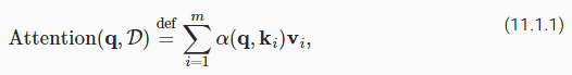
Clearly we would not have introduced a simple database here if it wasn’t for the purpose of explaining deep learning. Indeed, this leads to one of the most exciting concepts arguably introduced in deep learning in the past decade: the attention mechanism (Bahdanau et al., 2014). We will cover the specifics of its application to machine translation later. For now, simply consider the following: denote by Ddef={(k1,v1),…(km,vm)} a database of m tuples of keys and values. Moreover, denote by q a query. Then we can define the attention over D as where α(q,ki)∈ℝ (i=1,…,m) are scalar attention weights.
딥 러닝을 설명하기 위한 목적이 아니었다면 여기에 간단한 데이터베이스를 도입하지 않았을 것입니다. 실제로 이것은 지난 10년 동안 딥 러닝에 도입된 가장 흥미로운 개념 중 하나인 attention mechanism으로 이어집니다(Bahdanau et al., 2014). 나중에 기계 번역에 대한 응용 프로그램의 세부 사항을 다룰 것입니다. 지금은 간단히 다음을 고려하십시오. Ddef={(k1,v1),…(km,vm)} keys 와 values의 m 튜플 데이터베이스를 나타냅니다. 또한 쿼리를 q로 표시합니다. 그런 다음 α(q,ki)∈ℝ (i=1,…,m)이 스칼라 주의 가중치인 D에 대한 Attention를 정의할 수 있습니다.
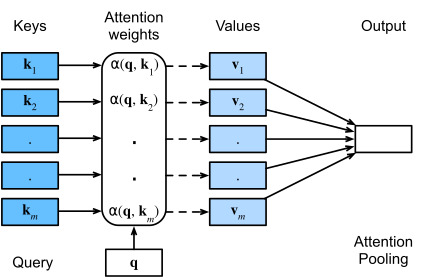
The operation itself is typically referred to as attention pooling. The name attention derives from the fact that the operation pays particular attention to the terms for which the weight α is significant (i.e., large). As such, the attention over D generates a linear combination of values contained in the database. In fact, this contains the above example as a special case where all but one weight is zero. We have a number of special cases:
작업 자체를 일반적으로 attention pooling이라고 합니다. attention 이라는 이름은 연산이 가중치 α가 중요한(즉, 큰) 용어에 특별한 attention 를 기울인다는 사실에서 유래합니다. 이와 같이 D에 대한 attention 은 데이터베이스에 포함된 values 의 선형 조합을 생성합니다. 사실 여기에는 하나를 제외하고 모두 가중치가 0인 특별한 경우로 위의 예가 포함되어 있습니다. 우리에게는 special cases가 많이 있습니다.
- The weights α(q,ki) are nonnegative. In this case the output of the attention mechanism is contained in the convex cone spanned by the values vi.
- weights α(q,ki)는 음수가 아닙니다. 이 경우 어텐션 메커니즘의 출력은 값 vi에 의해 확장되는 convex cone에 포함됩니다.
- The weights α(q,ki) form a convex combination, i.e., ∑iα(q,ki)=1 and α(q,ki)≥0 for all i. This is the most common setting in deep learning.
가중치 α(q,ki)는 convex combination, 즉 모든 i에 대해 ∑iα(q,ki)=1 이고 α(q,ki)≥0을 형성합니다. 이것은 딥 러닝에서 가장 일반적인 설정입니다. - Exactly one of the weights α(q,ki) is 1, while all others are 0. This is akin to a traditional database query.
- 가중치 α(q,ki) 중 정확히 하나는 1이고 나머지는 모두 0입니다. 이는 기존의 데이터베이스 쿼리와 유사합니다.
- All weights are equal, i.e., α(q,ki)=1/m for all i. This amounts to averaging across the entire database, also called average pooling in deep learning.
- 모든 가중치는 동일합니다. 즉, 모든 i에 대해 α(q,ki)=1/m입니다. 이는 딥 러닝에서 average pooling이라고도 하는 전체 데이터베이스의 평균입니다.
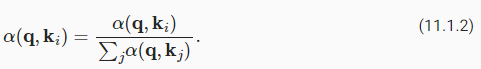
A common strategy to ensure that the weights sum up to 1 is to normalize them via
가중치 합이 1이 되도록 하는 일반적인 전략은 다음을 통해 가중치를 정규화하는 것입니다.
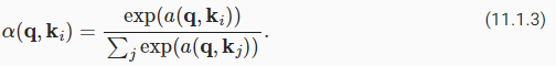
In particular, to ensure that the weights are also nonnegative, one can resort to exponentiation. This means that we can now pick any function α(q,k) and then apply the softmax operation used for multinomial models to it via
특히 가중치가 음수가 아닌 것을 확인하기 위해 지수화에 의지할 수 있습니다. 이것은 이제 우리가 어떤 함수 α(q,k)를 선택한 다음 다음을 통해 다항 모델에 사용되는 소프트맥스 연산을 적용할 수 있음을 의미합니다.
This operation is readily available in all deep learning frameworks. It is differentiable and its gradient never vanishes, all of which are desirable properties in a model. Note though, the attention mechanism introduced above is not the only option. For instance, we can design a non-differentiable attention model that can be trained using reinforcement learning methods (Mnih et al., 2014). As one would expect, training such a model is quite complex. Consequently the bulk of modern attention research follows the framework outlined in Fig. 11.1.1. We thus focus our exposition on this family of differentiable mechanisms.
이 operation 은 모든 딥 러닝 프레임워크에서 쉽게 사용할 수 있습니다. 미분 가능하고 기울기가 사라지지 않으며, 모두 모델에서 바람직한 속성(desirable properties)입니다. 그러나 위에서 소개한 어텐션 메커니즘이 유일한 옵션은 아닙니다. 예를 들어 강화 학습 방법(reinforcement learning methods)을 사용하여 훈련할 수 있는 미분할 수 없는 attention model을 설계할 수 있습니다(Mnih et al., 2014). 누구나 예상할 수 있듯이 그러한 모델을 교육하는 것은 상당히 복잡합니다. 결과적으로 현대 attention 연구의 대부분은 그림 11.1.1에 요약된 프레임워크를 따릅니다. 따라서 우리는 이 미분 가능한 메커니즘 계열에 대한 설명에 초점을 맞춥니다.
What is quite remarkable is that the actual “code” to execute on the set of keys and values, namely the query, can be quite concise, even though the space to operate on is significant. This is a desirable property for a network layer as it does not require too many parameters to learn. Just as convenient is the fact that attention can operate on arbitrarily large databases without the need to change the way the attention pooling operation is performed.
상당히 주목할 만한 점은 키와 값 세트를 통해 실행 할 코드, 즉 쿼리는 아주 중요합니다. 이것은 학습하는 데 너무 많은 매개변수가 필요하지 않기 때문에 network layer에 바람직한 속성입니다. attention pooling operation이 수행되는 방식을 변경할 필요 없이 attention 이 arbitrarily 큰 데이터베이스에서 작동할 수 있다는 사실도 편리합니다.
import torch
from d2l import torch as d2l
11.1.1. Visualization
One of the benefits of the attention mechanism is that it can be quite intuitive, particularly when the weights are nonnegative and sum to 1. In this case we might interpret large weights as a way for the model to select components of relevance. While this is a good intuition, it is important to remember that it is just that, an intuition. Regardless, we may want to visualize its effect on the given set of keys, when applying a variety of different queries. This function will come in handy later.
어텐션 메커니즘의 이점 중 하나는 특히 가중치가 음수가 아니고 합이 1일 때 매우 직관적(intuitive)일 수 있다는 것입니다. 이 경우 모델이 관련 구성 요소를 선택하는 방법으로 큰 가중치를 해석할 수 있습니다. 이것은 좋은 직감(intuition)이지만, 그것은 단지 직감이라는 것을 기억하는 것이 중요합니다. 그럼에도 불구하고 다양한 쿼리를 적용할 때 주어진 키 집합에 미치는 영향을 시각화하고 싶을 수 있습니다. 이 기능은 나중에 유용하게 활용될 것입니다.
#@save
def show_heatmaps(matrices, xlabel, ylabel, titles=None, figsize=(2.5, 2.5),
                  cmap='Reds'):
    """Show heatmaps of matrices."""
    d2l.use_svg_display()
    num_rows, num_cols, _, _ = matrices.shape
    fig, axes = d2l.plt.subplots(num_rows, num_cols, figsize=figsize,
                                 sharex=True, sharey=True, squeeze=False)
    for i, (row_axes, row_matrices) in enumerate(zip(axes, matrices)):
        for j, (ax, matrix) in enumerate(zip(row_axes, row_matrices)):
            pcm = ax.imshow(matrix.detach().numpy(), cmap=cmap)
            if i == num_rows - 1:
                ax.set_xlabel(xlabel)
            if j == 0:
                ax.set_ylabel(ylabel)
            if titles:
                ax.set_title(titles[j])
    fig.colorbar(pcm, ax=axes, shrink=0.6);
위 코드는 행렬들의 열화평면(heatmap)을 시각화하기 위한 함수를 정의하는 부분입니다. 이 함수를 사용하면 주어진 행렬들의 시각적인 표현을 생성하고 그릴 수 있습니다. heatmap은 행렬의 값들을 색상으로 표현하여 데이터의 패턴과 관계를 시각화하는 데 사용됩니다.
함수의 인자 설명:
- matrices: 시각화할 행렬들을 가지고 있는 4차원 텐서. (행 수, 열 수, 행 크기, 열 크기)의 형태를 가지며, 이 텐서에 있는 모든 행렬들을 heatmap으로 시각화합니다.
- xlabel: x축 레이블로 사용될 문자열.
- ylabel: y축 레이블로 사용될 문자열.
- titles: 열화평면 위에 표시될 제목들을 가지고 있는 리스트. 각 열화평면에 해당하는 제목을 지정할 수 있습니다.
- figsize: 생성된 열화평면의 크기를 지정하는 튜플.
- cmap: 색상 맵을 지정하는 문자열. heatmap의 색상을 결정합니다.
- d2l.use_svg_display(): SVG 형식으로 그림을 보여주는 설정을 적용합니다.
- num_rows, num_cols, _, _ = matrices.shape: 입력으로 받은 4차원 텐서의 형태에서 열화평면을 그릴 행과 열의 수를 가져옵니다.
- fig, axes = d2l.plt.subplots(...): 행렬들의 열화평면을 그릴 그림판과 서브플롯들을 생성합니다. num_rows x num_cols 크기의 서브플롯 그리드를 생성하며, figsize로 크기를 조절합니다.
- enumerate(zip(axes, matrices)): 서브플롯과 그에 해당하는 행렬을 하나씩 가져오는 반복문입니다.
- ax.imshow(...): 행렬을 heatmap으로 시각화합니다. imshow 함수에 행렬 데이터와 색상 맵(cmap)을 전달하여 heatmap을 그립니다.
- ax.set_xlabel(xlabel): x축 레이블을 설정합니다.
- ax.set_ylabel(ylabel): y축 레이블을 설정합니다.
- ax.set_title(titles[j]): 각 서브플롯의 제목을 설정합니다.
- fig.colorbar(...): 그림판에 색상 막대를 추가하여 heatmap의 값과 색상을 연결합니다.
이러한 단계들을 통해 show_heatmaps 함수는 입력으로 받은 행렬들을 열화평면으로 시각화합니다.
이 함수를 사용하면 주어진 행렬 데이터를 heatmap으로 시각화할 수 있습니다. 주로 머신러닝 모델의 가중치, 특성 맵, 그래디언트 등을 시각화하는 데 활용됩니다.
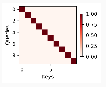
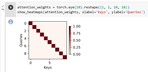
As a quick sanity check let’s visualize the identity matrix, representing a case where the attention weight is one only when the query and the key are the same.
quick sanity check로 쿼리와 키가 동일한 경우에만 어텐션 가중치가 1인 경우를 나타내는 항등 행렬(identity matrix)을 시각화해 보겠습니다.
11.1.2. Summary
The attention mechanism allows us to aggregate data from many (key, value) pairs. So far our discussion was quite abstract, simply describing a way to pool data. We have not explained yet where those mysterious queries, keys, and values might arise from. Some intuition might help here: for instance, in a regression setting, the query might correspond to the location where the regression should be carried out. The keys are the locations where past data was observed and the values are the (regression) values themselves. This is the so-called Nadaraya-Watson estimator (Nadaraya, 1964, Watson, 1964) that we will be studying in the next section.
어텐션 메커니즘을 통해 많은 (키, 값) 쌍의 데이터를 집계할 수 있습니다. 지금까지 우리의 논의는 매우 추상적이었고 단순히 데이터를 모으는 방법을 설명했습니다. 이러한 신비한 쿼리, 키 및 값이 어디서 발생할 수 있는지 아직 설명하지 않았습니다. 여기서 직관이 도움이 될 수 있습니다. 예를 들어 회귀 설정에서 쿼리는 회귀를 수행해야 하는 위치에 해당할 수 있습니다. 키는 과거 데이터가 관찰된 위치이고 값은 (회귀) 값 자체입니다. 이것은 소위 Nadaraya-Watson 추정기(Nadaraya, 1964, Watson, 1964)이며 다음 섹션에서 공부할 것입니다.
By design, the attention mechanism provides a differentiable means of control by which a neural network can select elements from a set and to construct an associated weighted sum over representations.
By design, attention mechanism은 신경망이 세트에서 elements 를 선택하고 representations에 대해 연관된 가중 합을 구성할 수 있는 미분 가능한 제어 수단을 제공합니다.
Nadaraya-Watson estimator란?
The Nadaraya-Watson estimator, often referred to as the Nadaraya-Watson kernel regression, is a non-parametric statistical method used for estimating the conditional expectation of a random variable given another random variable. It is commonly used in regression analysis and smoothing techniques.
나다라야-왓슨 추정기(Nadaraya-Watson estimator)는 종종 나다라야-왓슨 커널 회귀로 불리며, 랜덤 변수와 관련이 있는 다른 랜덤 변수를 기반으로 조건부 기대값을 추정하는 비모수적인 통계적 방법입니다. 이는 회귀 분석과 부드러운(smoothing) 기술에서 흔히 사용됩니다.
In simple terms, the Nadaraya-Watson estimator calculates the predicted value of a target variable based on a weighted average of observed values from the same dataset, where the weights are determined by a kernel function. This approach is particularly useful when dealing with noisy or complex data where a linear model may not be appropriate.
Mathematically, the Nadaraya-Watson estimator is expressed as:
간단하게 말하면, 나다라야-왓슨 추정기는 목표 변수의 예측 값을 계산하기 위해 같은 데이터 집합 내에서 관찰된 값들의 가중 평균을 사용하는데, 이때 가중치는 커널 함수에 의해 결정됩니다. 이 접근 방식은 선형 모델이 적절하지 않은 잡음이나 복잡한 데이터를 다룰 때 특히 유용합니다.
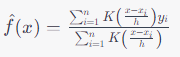
Where:
- is the estimated value of the target variable at point .
- 는 지점 에서 목표 변수의 추정된 값입니다.
- is the kernel function, which assigns weights to the data points based on their proximity to .
- 는 커널 함수로, 에 대한 가중치를 데이터 포인트에 할당합니다.
- are the observed values of the predictor variable.
- 는 예측 변수의 관찰 값입니다.
- are the corresponding observed values of the target variable.
- 는 해당하는 목표 변수의 관찰 값입니다.
- ℎ is the bandwidth parameter, which controls the width of the kernel and affects the smoothing level.
- 는 대역폭 파라미터로, 커널의 폭을 조절하고 부드러운 정도에 영향을 줍니다.
The Nadaraya-Watson estimator is a flexible and versatile tool for estimating relationships between variables without making strong assumptions about the underlying data distribution. It is commonly used in various fields, including machine learning, statistics, and data analysis.
나다라야-왓슨 추정기는 강력한 가정을 하지 않고 변수 간 관계를 추정하는 유연하고 다용도의 도구입니다. 이는 머신 러닝, 통계 및 데이터 분석을 포함한 여러 분야에서 흔히 사용됩니다.
https://youtu.be/lVZTVPzbEdo
https://youtu.be/FlI_1prDPpE
Where and how do you get Key, Value, and Query in Transformer?
In the Transformer architecture, the concepts of Key, Value, and Query are fundamental to the attention mechanism, which is a crucial component of both the encoder and decoder layers. They are used to compute the attention scores that determine how much focus should be given to different parts of the input sequence when generating the output sequence.
트랜스포머 아키텍처에서 'Key(키)', 'Value(값)', 'Query(쿼리)'는 어텐션 메커니즘의 기본 개념으로, 인코더와 디코더 레이어의 중요한 구성 요소입니다. 이들은 어텐션 점수를 계산하는 데 사용되며, 출력 시퀀스를 생성할 때 입력 시퀀스의 다른 부분에 얼마나 초점을 맞춰야 하는지를 결정합니다.
Here's how Key, Value, and Query are obtained in the Transformer:
트랜스포머에서 'Key(키)', 'Value(값)', 'Query(쿼리)'가 어떻게 얻어지는지에 대한 설명은 다음과 같습니다:
- Key (K): The Key vectors are derived from the input sequence and are used to represent the information in the context of each position. In the context of the self-attention mechanism, the Key vectors are obtained through a linear transformation of the input embeddings or the output of the previous layer.
키 벡터는 입력 시퀀스에서 파생되며 각 위치의 맥락을 나타내는 데 사용됩니다. 자기 어텐션 메커니즘의 맥락에서 키 벡터는 입력 임베딩 또는 이전 레이어의 출력의 선형 변환을 통해 얻어집니다. - Value (V): Similar to Keys, the Value vectors are also derived from the input sequence. They contain information about each position in the sequence and are used to provide context-aware representations. The Value vectors are obtained through another linear transformation of the input embeddings or the output of the previous layer.
키와 마찬가지로 값 벡터도 입력 시퀀스에서 파생됩니다. 각 위치의 정보를 포함하며 문맥에 민감한 표현을 제공합니다. 값 벡터는 입력 임베딩 또는 이전 레이어의 출력의 다른 선형 변환을 통해 얻어집니다. - Query (Q): The Query vectors represent the current position or token that the model is focusing on. These vectors are obtained in the same way as Keys and Values through a linear transformation of the input embeddings or the output of the previous layer.
쿼리 벡터는 모델이 주목하는 현재 위치나 토큰을 나타냅니다. 이 벡터들은 키와 값과 마찬가지로 입력 임베딩 또는 이전 레이어의 출력의 선형 변환을 통해 얻어집니다.
In the context of self-attention, the Key, Value, and Query vectors are transformed using different learned weight matrices for each of these components. Then, the attention scores between each Query and Key pair are computed, which quantify how well a Query relates to each Key. These attention scores are used to compute a weighted sum of the Value vectors, producing the attended output. This process is repeated across multiple attention heads in parallel, allowing the model to capture different aspects of context and relationships in the input sequence.
self-attention의 맥락에서 키, 값, 쿼리 벡터는 각 구성 요소에 대한 학습된 가중치 행렬을 적용하여 변환됩니다. 그런 다음 각 쿼리와 키 쌍 사이의 어텐션 점수가 계산되며, 각 쿼리가 각 키와 얼마나 관련이 있는지를 나타냅니다. 이 어텐션 점수는 값 벡터의 가중 합을 계산하는 데 사용되어 어텐드된 출력을 생성합니다. 이 프로세스는 병렬로 여러 어텐션 헤드에서 반복되며, 모델이 입력 시퀀스의 다양한 맥락과 관계를 포착할 수 있게 합니다.
In summary, the Key, Value, and Query vectors are obtained by applying linear transformations to the input embeddings or the output of the previous layer. They play a crucial role in the attention mechanism by allowing the model to attend to different parts of the input sequence while generating the output sequence.
요약하면, 'Key(키)', 'Value(값)', 'Query(쿼리)' 벡터는 입력 임베딩 또는 이전 레이어의 출력에 선형 변환을 적용하여 얻어집니다. 이들은 어텐션 메커니즘에서 핵심적인 역할을 하며 출력 시퀀스를 생성할 때 입력 시퀀스의 다른 부분에 주목할 수 있도록 해줍니다.
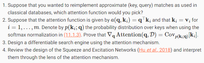
11.1.3. Exercises
'Dive into Deep Learning > D2L Attention Mechanisms and Transformer' 카테고리의 다른 글
| D2L - 11.9. Large-Scale Pretraining with Transformers (0) | 2023.08.10 |
|---|---|
| D2L - 11.8. Transformers for Vision (0) | 2023.08.10 |
| D2L - 11.7. The Transformer Architecture (0) | 2023.08.09 |
| D2L - 11.6. Self-Attention and Positional Encoding (0) | 2023.08.09 |
| D2L - 11.5. Multi-Head Attention (0) | 2023.08.08 |
| D2L - 11.4. The Bahdanau Attention Mechanism (0) | 2023.08.08 |
| D2L - 11.3. Attention Scoring Functions (0) | 2023.08.07 |
| D2L - 11.2. Attention Pooling by Similarity (0) | 2023.08.06 |
| D2L - 11. Attention Mechanisms and Transformers (0) | 2023.08.03 |