반응형
블로그 이미지
개발자로서 현장에서 일하면서 새로 접하는 기술들이나 알게된 정보 등을 정리하기 위한 블로그입니다. 운 좋게 미국에서 큰 회사들의 프로젝트에서 컬설턴트로 일하고 있어서 새로운 기술들을 접할 기회가 많이 있습니다. 미국의 IT 프로젝트에서 사용되는 툴들에 대해 많은 분들과 정보를 공유하고 싶습니다.
솔웅

최근에 올라온 글

최근에 달린 댓글

최근에 받은 트랙백

글 보관함

카테고리


반응형

16.7. Natural Language Inference: Fine-Tuning BERT — Dive into Deep Learning 1.0.3 documentation (d2l.ai)


16.7. Natural Language Inference: Fine-Tuning BERT — Dive into Deep Learning 1.0.3 documentation


d2l.ai


16.7. Natural Language Inference: Fine-Tuning BERT


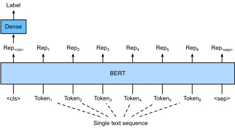
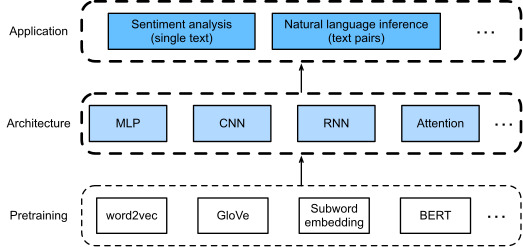
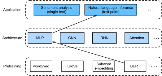
In earlier sections of this chapter, we have designed an attention-based architecture (in Section 16.5) for the natural language inference task on the SNLI dataset (as described in Section 16.4). Now we revisit this task by fine-tuning BERT. As discussed in Section 16.6, natural language inference is a sequence-level text pair classification problem, and fine-tuning BERT only requires an additional MLP-based architecture, as illustrated in Fig. 16.7.1.


이 장의 이전 섹션에서 우리는 SNLI 데이터 세트(섹션 16.4에서 설명)에 대한 자연어 추론 작업을 위한 attention-based architecture(섹션 16.5)를 설계했습니다. 이제 BERT를 미세 조정하여 이 작업을 다시 살펴보겠습니다. 섹션 16.6에서 설명한 것처럼 자연어 추론은 시퀀스 수준 텍스트 쌍 분류 문제이며 BERT를 미세 조정하려면 그림 16.7.1에 설명된 것처럼 추가적인 MLP 기반 아키텍처만 필요합니다.


Fig. 16.7.1  This section feeds pretrained BERT to an MLP-based architecture for natural language inference.


In this section, we will download a pretrained small version of BERT, then fine-tune it for natural language inference on the SNLI dataset.


이 섹션에서는 사전 훈련된 BERT의 작은 버전을 다운로드한 다음 SNLI 데이터 세트에 대한 자연어 추론을 위해 미세 조정합니다.


import json
import multiprocessing
import os
import torch
from torch import nn
from d2l import torch as d2l


16.7.1. Loading Pretrained BERT


We have explained how to pretrain BERT on the WikiText-2 dataset in Section 15.9 and Section 15.10 (note that the original BERT model is pretrained on much bigger corpora). As discussed in Section 15.10, the original BERT model has hundreds of millions of parameters. In the following, we provide two versions of pretrained BERT: “bert.base” is about as big as the original BERT base model that requires a lot of computational resources to fine-tune, while “bert.small” is a small version to facilitate demonstration.


d2l.DATA_HUB['bert.base'] = (d2l.DATA_URL + 'bert.base.torch.zip',
                             '225d66f04cae318b841a13d32af3acc165f253ac')
d2l.DATA_HUB['bert.small'] = (d2l.DATA_URL + 'bert.small.torch.zip',
                              'c72329e68a732bef0452e4b96a1c341c8910f81f')

이 코드는 데이터 저장소(DATA_HUB)에 두 개의 BERT(Bidirectional Encoder Representations from Transformers) 모델에 대한 정보를 추가하는 역할을 합니다. BERT는 자연어 처리 작업에 사용되는 사전 훈련된 언어 모델 중 하나로, 큰 텍스트 코퍼스에서 학습된 후 다양한 NLP 작업에 전이 학습(transfer learning)을 적용할 수 있도록 훈련된 모델입니다.

  • 'bert.base': 이 키는 큰 규모의 BERT 모델에 대한 정보를 나타냅니다. 해당 모델의 체크포인트 파일은 bert.base.torch.zip로 저장되어 있으며, 해당 파일을 다운로드하여 모델을 로드할 수 있습니다. 이 모델은 큰 언어 모델이기 때문에 자연어 처리 작업에 높은 성능을 제공할 것으로 기대됩니다.
  • 'bert.small': 이 키는 작은 규모의 BERT 모델에 대한 정보를 나타냅니다. 작은 모델은 더 가벼우며 계산 비용이 적게 들지만, 큰 모델보다는 성능이 낮을 수 있습니다. 이 모델은 자연어 처리 작업에 적합한 자원이 제한된 환경에서 사용될 수 있습니다.

따라서 이 코드는 데이터 저장소에서 BERT 모델의 체크포인트 파일을 다운로드하고 이를 사용하여 BERT 모델을 로드할 수 있도록 필요한 정보를 설정합니다.


Either pretrained BERT model contains a “vocab.json” file that defines the vocabulary set and a “pretrained.params” file of the pretrained parameters. We implement the following load_pretrained_model function to load pretrained BERT parameters.


사전 훈련된 BERT 모델에는 어휘 세트를 정의하는 "vocab.json" 파일과 사전 훈련된 매개변수의 "pretrained.params" 파일이 포함되어 있습니다. 사전 훈련된 BERT 매개변수를 로드하기 위해 다음 load_pretrained_model 함수를 구현합니다.


def load_pretrained_model(pretrained_model, num_hiddens, ffn_num_hiddens,
                          num_heads, num_blks, dropout, max_len, devices):
    data_dir = d2l.download_extract(pretrained_model)
    # Define an empty vocabulary to load the predefined vocabulary
    vocab = d2l.Vocab()
    vocab.idx_to_token = json.load(open(os.path.join(data_dir, 'vocab.json')))
    vocab.token_to_idx = {token: idx for idx, token in enumerate(
        vocab.idx_to_token)}
    bert = d2l.BERTModel(
        len(vocab), num_hiddens, ffn_num_hiddens=ffn_num_hiddens, num_heads=4,
        num_blks=2, dropout=0.2, max_len=max_len)
    # Load pretrained BERT parameters
    bert.load_state_dict(torch.load(os.path.join(data_dir,
                                                 'pretrained.params')))
    return bert, vocab

이 함수는 다음과 같은 역할을 합니다:

  1. pretrained_model: 미리 학습된 BERT 모델의 이름 또는 경로를 나타냅니다.
  2. num_hiddens: BERT 모델의 은닉 상태 크기를 나타냅니다.
  3. ffn_num_hiddens: BERT 모델의 Feedforward 네트워크에서의 은닉 상태 크기를 나타냅니다.
  4. num_heads: BERT 모델의 어텐션 헤드 개수를 나타냅니다.
  5. num_blks: BERT 모델의 어텐션 블록 수를 나타냅니다.
  6. dropout: 드롭아웃 비율을 나타냅니다.
  7. max_len: 입력 시퀀스의 최대 길이를 나타냅니다.
  8. devices: 사용할 디바이스 목록입니다.

함수는 다음 단계로 수행됩니다:

  • pretrained_model을 통해 지정된 미리 학습된 BERT 모델을 다운로드하고 압축을 해제합니다.
  • 빈 어휘 사전(vocab)을 정의하고, 미리 정의된 어휘 파일을 로드하여 이 어휘 사전을 채웁니다.
  • BERT 모델을 지정된 구성 및 어휘 사전을 사용하여 초기화합니다.
  • 미리 학습된 BERT 모델의 파라미터를 로드하여 BERT 모델을 미리 학습된 상태로 설정합니다.
  • 초기화된 BERT 모델과 어휘 사전을 반환합니다.

이 함수를 호출하면 미리 학습된 BERT 모델과 해당 어휘 사전이 반환됩니다. 이 모델을 사용하여 다양한 자연어 처리 작업을 수행할 수 있습니다.


To facilitate demonstration on most of machines, we will load and fine-tune the small version (“bert.small”) of the pretrained BERT in this section. In the exercise, we will show how to fine-tune the much larger “bert.base” to significantly improve the testing accuracy.


대부분의 머신에서 시연을 용이하게 하기 위해 이 섹션에서는 사전 훈련된 BERT의 작은 버전("bert.small")을 로드하고 미세 조정합니다. 이 연습에서는 훨씬 더 큰 "bert.base"를 미세 조정하여 테스트 정확도를 크게 향상시키는 방법을 보여줍니다.


devices = d2l.try_all_gpus()
bert, vocab = load_pretrained_model(
    'bert.small', num_hiddens=256, ffn_num_hiddens=512, num_heads=4,
    num_blks=2, dropout=0.1, max_len=512, devices=devices)

위의 코드는 BERT 모델을 불러오고 설정하는 작업을 수행합니다. 

  1. devices = d2l.try_all_gpus(): 이 코드는 가능한 모든 GPU 디바이스를 사용 가능한 경우 가져옵니다. 이것은 여러 GPU에서 BERT 모델을 병렬로 학습하거나 추론할 때 사용됩니다.
  2. load_pretrained_model(...): 이 함수는 앞서 정의한 load_pretrained_model 함수를 호출하여 미리 학습된 BERT 모델을 로드하고 설정합니다.
    • 'bert.small': 불러올 미리 학습된 BERT 모델의 이름 또는 경로를 나타냅니다.
    • num_hiddens=256: BERT 모델의 은닉 상태 크기를 설정합니다.
    • ffn_num_hiddens=512: BERT 모델의 Feedforward 네트워크에서의 은닉 상태 크기를 설정합니다.
    • num_heads=4: BERT 모델의 어텐션 헤드 개수를 설정합니다.
    • num_blks=2: BERT 모델의 어텐션 블록 수를 설정합니다.
    • dropout=0.1: 드롭아웃 비율을 설정합니다.
    • max_len=512: 입력 시퀀스의 최대 길이를 설정합니다.
    • devices=devices: 사용할 GPU 디바이스 목록을 전달합니다.

이 코드를 실행하면 bert 변수에는 설정된 BERT 모델이 로드되며, vocab 변수에는 어휘 사전이 로드됩니다. 이제 bert 모델을 사용하여 다양한 자연어 처리 작업을 수행할 수 있습니다.

Downloading ../data/bert.small.torch.zip from http://d2l-data.s3-accelerate.amazonaws.com/bert.small.torch.zip...


16.7.2. The Dataset for Fine-Tuning BERT


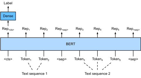
For the downstream task natural language inference on the SNLI dataset, we define a customized dataset class SNLIBERTDataset. In each example, the premise and hypothesis form a pair of text sequence and is packed into one BERT input sequence as depicted in Fig. 16.6.2. Recall Section 15.8.4 that segment IDs are used to distinguish the premise and the hypothesis in a BERT input sequence. With the predefined maximum length of a BERT input sequence (max_len), the last token of the longer of the input text pair keeps getting removed until max_len is met. To accelerate generation of the SNLI dataset for fine-tuning BERT, we use 4 worker processes to generate training or testing examples in parallel.


SNLI 데이터 세트에 대한 다운스트림 작업 자연어 추론을 위해 맞춤형 데이터 세트 클래스 SNLIBERTDataset를 정의합니다. 각 예에서 전제와 가설은 한 쌍의 텍스트 시퀀스를 형성하고 그림 16.6.2에 설명된 대로 하나의 BERT 입력 시퀀스로 압축됩니다. BERT 입력 시퀀스에서 전제와 가설을 구별하기 위해 세그먼트 ID가 사용된다는 섹션 15.8.4를 상기하세요. BERT 입력 시퀀스의 사전 정의된 최대 길이(max_len)를 사용하면 max_len이 충족될 때까지 더 긴 입력 텍스트 쌍의 마지막 토큰이 계속 제거됩니다. BERT 미세 조정을 위한 SNLI 데이터 세트 생성을 가속화하기 위해 4개의 작업자 프로세스를 사용하여 훈련 또는 테스트 예제를 병렬로 생성합니다.


class SNLIBERTDataset(torch.utils.data.Dataset):
    def __init__(self, dataset, max_len, vocab=None):
        all_premise_hypothesis_tokens = [[
            p_tokens, h_tokens] for p_tokens, h_tokens in zip(
            *[d2l.tokenize([s.lower() for s in sentences])
              for sentences in dataset[:2]])]

        self.labels = torch.tensor(dataset[2])
        self.vocab = vocab
        self.max_len = max_len
        (self.all_token_ids, self.all_segments,
         self.valid_lens) = self._preprocess(all_premise_hypothesis_tokens)
        print('read ' + str(len(self.all_token_ids)) + ' examples')

    def _preprocess(self, all_premise_hypothesis_tokens):
        pool = multiprocessing.Pool(4)  # Use 4 worker processes
        out = pool.map(self._mp_worker, all_premise_hypothesis_tokens)
        all_token_ids = [
            token_ids for token_ids, segments, valid_len in out]
        all_segments = [segments for token_ids, segments, valid_len in out]
        valid_lens = [valid_len for token_ids, segments, valid_len in out]
        return (torch.tensor(all_token_ids, dtype=torch.long),
                torch.tensor(all_segments, dtype=torch.long),
                torch.tensor(valid_lens))

    def _mp_worker(self, premise_hypothesis_tokens):
        p_tokens, h_tokens = premise_hypothesis_tokens
        self._truncate_pair_of_tokens(p_tokens, h_tokens)
        tokens, segments = d2l.get_tokens_and_segments(p_tokens, h_tokens)
        token_ids = self.vocab[tokens] + [self.vocab['<pad>']] \
                             * (self.max_len - len(tokens))
        segments = segments + [0] * (self.max_len - len(segments))
        valid_len = len(tokens)
        return token_ids, segments, valid_len

    def _truncate_pair_of_tokens(self, p_tokens, h_tokens):
        # Reserve slots for '<CLS>', '<SEP>', and '<SEP>' tokens for the BERT
        # input
        while len(p_tokens) + len(h_tokens) > self.max_len - 3:
            if len(p_tokens) > len(h_tokens):
                p_tokens.pop()
            else:
                h_tokens.pop()

    def __getitem__(self, idx):
        return (self.all_token_ids[idx], self.all_segments[idx],
                self.valid_lens[idx]), self.labels[idx]

    def __len__(self):
        return len(self.all_token_ids)

이 코드는 SNLI 데이터셋을 BERT 모델의 입력 형식에 맞게 전처리하는 데 사용되는 SNLIBERTDataset 클래스를 정의합니다. 이 클래스는 PyTorch의 torch.utils.data.Dataset 클래스를 상속하며, 데이터를 로드하고 전처리하는 역할을 합니다. 


  1. __init__(self, dataset, max_len, vocab=None): 이 클래스의 생성자는 다음과 같은 매개변수를 받습니다.
    • dataset: SNLI 데이터셋.
    • max_len: BERT 입력 시퀀스의 최대 길이.
    • vocab: 어휘 사전 (생략 가능).
  2. _preprocess(self, all_premise_hypothesis_tokens): 이 메서드는 데이터셋을 전처리하고 BERT 모델 입력에 맞게 변환합니다. 멀티프로세스를 사용하여 병렬로 처리하며, BERT 모델에 입력으로 들어갈 토큰 ID, 세그먼트 ID, 유효한 길이를 반환합니다.
  3. _mp_worker(self, premise_hypothesis_tokens): 이 메서드는 멀티프로세스 작업을 위해 호출되며, 입력으로 주어진 전제와 가설 문장의 토큰을 BERT 입력 형식에 맞게 전처리합니다.
  4. _truncate_pair_of_tokens(self, p_tokens, h_tokens): 이 메서드는 전제와 가설 문장의 토큰 길이가 max_len을 초과하지 않도록 자르는 역할을 합니다.
  5. __getitem__(self, idx): 이 메서드는 데이터셋에서 특정 인덱스 idx에 해당하는 데이터를 반환합니다. 이 데이터는 BERT 모델의 입력과 레이블을 포함합니다.
  6. __len__(self): 이 메서드는 데이터셋의 총 데이터 수를 반환합니다.

이 클래스를 사용하면 SNLI 데이터를 BERT 모델에 입력으로 제공하기 위한 데이터셋을 쉽게 생성할 수 있습니다.


After downloading the SNLI dataset, we generate training and testing examples by instantiating the SNLIBERTDataset class. Such examples will be read in minibatches during training and testing of natural language inference.


SNLI 데이터 세트를 다운로드한 후 SNLIBERTDataset 클래스를 인스턴스화하여 훈련 및 테스트 예제를 생성합니다. 이러한 예제는 자연어 추론을 훈련하고 테스트하는 동안 미니배치로 읽혀집니다.


# Reduce `batch_size` if there is an out of memory error. In the original BERT
# model, `max_len` = 512
batch_size, max_len, num_workers = 512, 128, d2l.get_dataloader_workers()
data_dir = d2l.download_extract('SNLI')
train_set = SNLIBERTDataset(d2l.read_snli(data_dir, True), max_len, vocab)
test_set = SNLIBERTDataset(d2l.read_snli(data_dir, False), max_len, vocab)
train_iter = torch.utils.data.DataLoader(train_set, batch_size, shuffle=True,
                                   num_workers=num_workers)
test_iter = torch.utils.data.DataLoader(test_set, batch_size,
                                  num_workers=num_workers)

이 코드는 BERT 모델을 사용하여 SNLI 데이터셋을 학습하기 위한 데이터 로딩 및 전처리 부분을 담당합니다.

  1. batch_size, max_len, num_workers 설정: 이 부분에서는 배치 크기(batch_size), 최대 시퀀스 길이(max_len), 그리고 데이터 로더에 사용할 워커 수(num_workers)를 설정합니다. 원래 BERT 모델에서는 max_len을 512로 사용하나, 메모리 부족 문제가 발생할 경우 이 값을 낮출 수 있습니다.
  2. 데이터 다운로드 및 전처리: data_dir 변수에 SNLI 데이터셋을 다운로드하고 압축을 해제합니다. 그 후, train_set과 test_set을 각각 SNLIBERTDataset 클래스로 초기화합니다. 이 때, max_len은 지정한 값으로 설정하고, vocab은 미리 로드한 어휘 사전을 사용합니다.
  3. 데이터 로더 생성: train_set과 test_set을 기반으로 데이터 로더(train_iter와 test_iter)를 생성합니다. 데이터 로더는 미니배치를 생성하고 데이터를 셔플하며, 병렬로 데이터를 로드하기 위해 num_workers를 사용합니다.

이렇게 설정된 데이터 로더를 사용하여 BERT 모델을 학습하고 평가할 수 있습니다.

read 549367 examples
read 9824 examples


16.7.3. Fine-Tuning BERT

As Fig. 16.6.2 indicates, fine-tuning BERT for natural language inference requires only an extra MLP consisting of two fully connected layers (see self.hidden and self.output in the following BERTClassifier class). This MLP transforms the BERT representation of the special “<cls>” token, which encodes the information of both the premise and the hypothesis, into three outputs of natural language inference: entailment, contradiction, and neutral.


그림 16.6.2에서 알 수 있듯이 자연어 추론을 위해 BERT를 미세 조정하려면 두 개의 완전히 연결된 레이어로 구성된 추가 MLP만 필요합니다(다음 BERTClassifier 클래스의 self.hidden 및 self.output 참조). 이 MLP는 전제와 가설 모두의 정보를 인코딩하는 특수 "<cls>" 토큰의 BERT 표현을 수반, 모순 및 중립의 세 가지 자연어 추론 출력으로 변환합니다.


class BERTClassifier(nn.Module):
    def __init__(self, bert):
        super(BERTClassifier, self).__init__()
        self.encoder = bert.encoder
        self.hidden = bert.hidden
        self.output = nn.LazyLinear(3)

    def forward(self, inputs):
        tokens_X, segments_X, valid_lens_x = inputs
        encoded_X = self.encoder(tokens_X, segments_X, valid_lens_x)
        return self.output(self.hidden(encoded_X[:, 0, :]))

이 모델은 다음과 같은 구조를 가집니다:

  1. self.encoder: BERT 모델의 인코더 부분을 가져와서 저장합니다. 이는 입력 데이터에 대한 특성 추출을 담당합니다.
  2. self.hidden: BERT 모델의 은닉 상태 부분을 가져와서 저장합니다. 이 부분은 모델의 내부 표현을 다룹니다.
  3. self.output: 감정 분류를 위한 출력 레이어로, 3개의 클래스로 분류하기 위한 선형 레이어입니다.

forward 메서드에서는 다음과 같은 과정을 거칩니다:

  1. 입력 데이터(inputs)를 받습니다. 이 입력 데이터는 토큰, 세그먼트, 유효한 길이로 이루어져 있습니다.
  2. 입력 데이터를 BERT 인코더(self.encoder)를 통해 처리하여 인코딩된 데이터(encoded_X)를 얻습니다.
  3. 인코딩된 데이터 중 첫 번째 토큰(encoded_X[:, 0, :])의 표현을 가져와서 이를 출력 레이어(self.output)에 입력합니다.
  4. 출력 레이어는 입력 표현을 활용하여 감정 분류를 수행하고 결과를 반환합니다.

이렇게 정의된 BERTClassifier 모델은 BERT를 기반으로 하여 텍스트 감정 분류를 수행하는 모델입니다.


In the following, the pretrained BERT model bert is fed into the BERTClassifier instance net for the downstream application. In common implementations of BERT fine-tuning, only the parameters of the output layer of the additional MLP (net.output) will be learned from scratch. All the parameters of the pretrained BERT encoder (net.encoder) and the hidden layer of the additional MLP (net.hidden) will be fine-tuned.


다음에서는 사전 훈련된 BERT 모델 bert가 다운스트림 애플리케이션을 위한 BERTClassifier 인스턴스 net에 공급됩니다. BERT 미세 조정의 일반적인 구현에서는 추가 MLP(net.output)의 출력 레이어 매개변수만 처음부터 학습됩니다. 사전 훈련된 BERT 인코더(net.encoder)의 모든 매개변수와 추가 MLP(net.hidden)의 숨겨진 계층이 미세 조정됩니다.


net = BERTClassifier(bert)

이 코드는 앞서 정의한 BERTClassifier 클래스를 사용하여 실제 BERT 모델을 텍스트 감정 분류를 위한 모델로 초기화하는 부분입니다.

여기서 net은 BERTClassifier 클래스의 인스턴스로, bert는 미리 학습된 BERT 모델을 의미합니다. 이 코드를 실행하면 net은 텍스트 감정 분류를 위한 모델로 설정되며, 이 모델은 BERT의 인코더와 은닉 상태를 활용하여 입력된 텍스트 데이터를 분류합니다.

즉, net을 사용하면 미리 학습된 BERT 모델을 감정 분류 작업에 활용할 수 있게 됩니다.


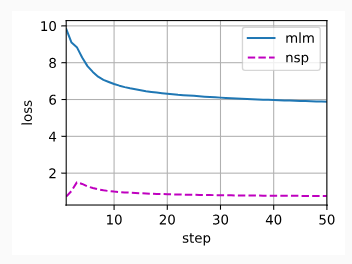
Recall that in Section 15.8 both the MaskLM class and the NextSentencePred class have parameters in their employed MLPs. These parameters are part of those in the pretrained BERT model bert, and thus part of parameters in net. However, such parameters are only for computing the masked language modeling loss and the next sentence prediction loss during pretraining. These two loss functions are irrelevant to fine-tuning downstream applications, thus the parameters of the employed MLPs in MaskLM and NextSentencePred are not updated (staled) when BERT is fine-tuned.


섹션 15.8에서 MaskLM 클래스와 NextSentencePred 클래스 모두 사용된 MLP에 매개변수를 가지고 있다는 점을 기억하세요. 이러한 매개변수는 사전 훈련된 BERT 모델 bert의 매개변수의 일부이므로 net의 매개변수의 일부입니다. 그러나 이러한 매개변수는 사전 훈련 중 마스크된 언어 모델링 손실과 다음 문장 예측 손실을 계산하는 데만 사용됩니다. 이 두 가지 손실 함수는 다운스트림 애플리케이션을 미세 조정하는 것과 관련이 없으므로 BERT가 미세 조정될 때 MaskLM 및 NextSentencePred에 사용된 MLP의 매개변수가 업데이트(정지)되지 않습니다.


To allow parameters with stale gradients, the flag ignore_stale_grad=True is set in the step function of d2l.train_batch_ch13. We use this function to train and evaluate the model net using the training set (train_iter) and the testing set (test_iter) of SNLI. Due to the limited computational resources, the training and testing accuracy can be further improved: we leave its discussions in the exercises.


오래된 그래디언트가 있는 매개변수를 허용하려면 d2l.train_batch_ch13의 단계 함수에ignore_stale_grad=True 플래그가 설정됩니다. 우리는 이 함수를 사용하여 SNLI의 훈련 세트(train_iter)와 테스트 세트(test_iter)를 사용하여 모델 네트워크를 훈련하고 평가합니다. 제한된 계산 리소스로 인해 훈련 및 테스트 정확도가 더욱 향상될 수 있습니다. 이에 대한 논의는 연습에 남겨두겠습니다.


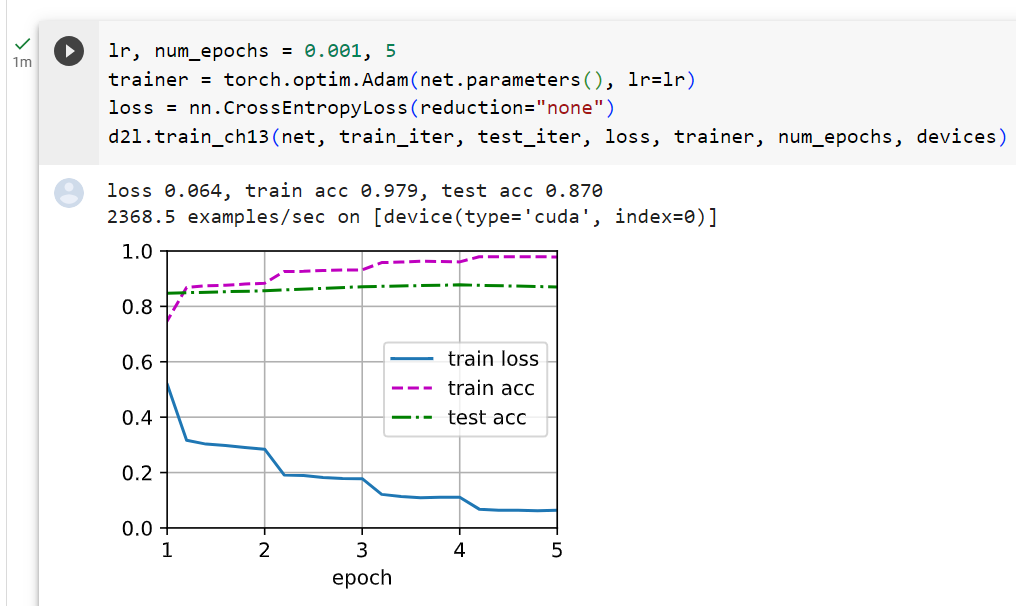
lr, num_epochs = 1e-4, 5
trainer = torch.optim.Adam(net.parameters(), lr=lr)
loss = nn.CrossEntropyLoss(reduction='none')
net(next(iter(train_iter))[0])
d2l.train_ch13(net, train_iter, test_iter, loss, trainer, num_epochs, devices)

이 코드는 BERT 모델을 텍스트 감정 분류 작업에 학습시키는 부분입니다.

  1. lr, num_epochs 변수는 학습률 (lr)과 학습 에포크 수 (num_epochs)를 설정합니다. lr은 0.0001로 설정되어 있으며, 학습률은 모델 가중치 업데이트에 사용되는 값입니다. num_epochs는 5로 설정되어 있으며, 데이터셋을 5번 반복하여 학습합니다.
  2. trainer 변수는 torch.optim.Adam 옵티마이저를 초기화합니다. 이 옵티마이저는 모델의 파라미터를 업데이트하는 데 사용됩니다.
  3. loss 변수는 nn.CrossEntropyLoss를 초기화합니다. 이 손실 함수는 다중 클래스 분류 작업에서 사용되며, 모델의 출력과 실제 레이블 간의 크로스 엔트로피 손실을 계산합니다. reduction='none'으로 설정되어 있으므로 손실을 각 샘플에 대한 개별 손실로 계산합니다.
  4. net(next(iter(train_iter))[0]) 코드는 학습 데이터의 첫 번째 미니배치를 사용하여 모델을 실행하고 출력을 확인하는 용도로 사용됩니다.
  5. d2l.train_ch13 함수를 호출하여 모델을 학습합니다. 이 함수는 모델, 학습 데이터 반복자, 테스트 데이터 반복자, 손실 함수, 옵티마이저, 학습 에포크 수, 그리고 디바이스를 입력으로 받아 모델을 학습하고 학습 결과를 시각화합니다. 이를 통해 BERT 모델이 텍스트 감정 분류 작업을 수행하도록 학습됩니다.

이러한 단계를 통해 BERT 모델이 주어진 데이터에 대해 감정 분류 작업을 수행하도록 학습됩니다.

loss 0.520, train acc 0.791, test acc 0.786
10588.8 examples/sec on [device(type='cuda', index=0), device(type='cuda', index=1)]
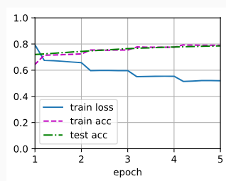
 

16.7.4. Summary

  • We can fine-tune the pretrained BERT model for downstream applications, such as natural language inference on the SNLI dataset.
  • SNLI 데이터세트에 대한 자연어 추론과 같은 다운스트림 애플리케이션을 위해 사전 훈련된 BERT 모델을 미세 조정할 수 있습니다.
  • During fine-tuning, the BERT model becomes part of the model for the downstream application. Parameters that are only related to pretraining loss will not be updated during fine-tuning.
  • 미세 조정 중에 BERT 모델은 다운스트림 애플리케이션을 위한 모델의 일부가 됩니다. 사전 훈련 손실에만 관련된 매개변수는 미세 조정 중에 업데이트되지 않습니다.


16.7.5. Exercises

  1. Fine-tune a much larger pretrained BERT model that is about as big as the original BERT base model if your computational resource allows. Set arguments in the load_pretrained_model function as: replacing ‘bert.small’ with ‘bert.base’, increasing values of num_hiddens=256, ffn_num_hiddens=512, num_heads=4, and num_blks=2 to 768, 3072, 12, and 12, respectively. By increasing fine-tuning epochs (and possibly tuning other hyperparameters), can you get a testing accuracy higher than 0.86?
  2. How to truncate a pair of sequences according to their ratio of length? Compare this pair truncation method and the one used in the SNLIBERTDataset class. What are their pros and cons?


반응형


반응형

16.6. Fine-Tuning BERT for Sequence-Level and Token-Level Applications — Dive into Deep Learning 1.0.3 documentation (d2l.ai)


16.6. Fine-Tuning BERT for Sequence-Level and Token-Level Applications — Dive into Deep Learning 1.0.3 documentation


d2l.ai


In the previous sections of this chapter, we have designed different models for natural language processing applications, such as based on RNNs, CNNs, attention, and MLPs. These models are helpful when there is space or time constraint, however, crafting a specific model for every natural language processing task is practically infeasible. In Section 15.8, we introduced a pretraining model, BERT, that requires minimal architecture changes for a wide range of natural language processing tasks. On the one hand, at the time of its proposal, BERT improved the state of the art on various natural language processing tasks. On the other hand, as noted in Section 15.10, the two versions of the original BERT model come with 110 million and 340 million parameters. Thus, when there are sufficient computational resources, we may consider fine-tuning BERT for downstream natural language processing applications.


이 장의 이전 섹션에서는 RNN, CNN, Attention 및 MLP를 기반으로 하는 자연어 처리 애플리케이션을 위한 다양한 모델을 설계했습니다. 이러한 모델은 공간이나 시간 제약이 있을 때 유용하지만 모든 자연어 처리 작업에 대한 특정 모델을 만드는 것은 사실상 불가능합니다. 섹션 15.8에서는 광범위한 자연어 처리 작업에 대해 최소한의 아키텍처 변경이 필요한 사전 훈련 모델인 BERT를 소개했습니다. 한편, BERT는 제안 당시 다양한 자연어 처리 작업에 대한 최신 기술을 개선했습니다. 반면에 섹션 15.10에서 언급했듯이 원래 BERT 모델의 두 가지 버전에는 1억 1천만 개와 3억 4천만 개의 매개 변수가 있습니다. 따라서 계산 리소스가 충분할 경우 다운스트림 자연어 처리 애플리케이션을 위해 BERT를 미세 조정하는 것을 고려할 수 있습니다.


In the following, we generalize a subset of natural language processing applications as sequence-level and token-level. On the sequence level, we introduce how to transform the BERT representation of the text input to the output label in single text classification and text pair classification or regression. On the token level, we will briefly introduce new applications such as text tagging and question answering and shed light on how BERT can represent their inputs and get transformed into output labels. During fine-tuning, the “minimal architecture changes” required by BERT across different applications are the extra fully connected layers. During supervised learning of a downstream application, parameters of the extra layers are learned from scratch while all the parameters in the pretrained BERT model are fine-tuned.


다음에서는 자연어 처리 애플리케이션의 하위 집합을 시퀀스 수준 및 토큰 수준으로 일반화합니다. 시퀀스 수준에서는 단일 텍스트 분류 및 텍스트 쌍 분류 또는 회귀에서 텍스트 입력의 BERT 표현을 출력 레이블로 변환하는 방법을 소개합니다. 토큰 수준에서는 텍스트 태깅 및 질문 답변과 같은 새로운 애플리케이션을 간략하게 소개하고 BERT가 입력을 표현하고 출력 레이블로 변환하는 방법을 조명합니다. 미세 조정 중에 다양한 애플리케이션 전반에 걸쳐 BERT에 필요한 "최소 아키텍처 변경"은 추가로 완전히 연결된 레이어입니다. 다운스트림 애플리케이션의 지도 학습 중에 추가 레이어의 매개변수는 사전 학습된 BERT 모델의 모든 매개변수가 미세 조정되는 동안 처음부터 학습됩니다.


16.6.1. Single Text Classification

Single text classification takes a single text sequence as input and outputs its classification result. Besides sentiment analysis that we have studied in this chapter, the Corpus of Linguistic Acceptability (CoLA) is also a dataset for single text classification, judging whether a given sentence is grammatically acceptable or not (Warstadt et al., 2019). For instance, “I should study.” is acceptable but “I should studying.” is not.


단일 텍스트 분류는 단일 텍스트 시퀀스를 입력으로 사용하고 해당 분류 결과를 출력합니다. 이 장에서 연구한 감정 분석 외에도 CoLA(언어적 수용성 코퍼스)는 주어진 문장이 문법적으로 수용 가능한지 여부를 판단하는 단일 텍스트 분류를 위한 데이터 세트이기도 합니다(Warstadt et al., 2019). 예를 들어, “I should study.” 는 괜찮지만 “I should studying” 문법적으로 틀리다.


Fig. 16.6.1&nbsp; Fine-tuning BERT for single text classification applications, such as sentiment analysis and testing linguistic acceptability. Suppose that the input single text has six tokens.&nbsp;그림 16.6.1&nbsp; 감정 분석 및 언어 수용성 테스트와 같은 단일 텍스트 분류 애플리케이션을 위해 BERT를 미세 조정합니다. 입력 단일 텍스트에 6개의 토큰이 있다고 가정합니다.

Section 15.8 describes the input representation of BERT. The BERT input sequence unambiguously represents both single text and text pairs, where the special classification token “<cls>” is used for sequence classification and the special classification token “<sep>” marks the end of single text or separates a pair of text. As shown in Fig. 16.6.1, in single text classification applications, the BERT representation of the special classification token “<cls>” encodes the information of the entire input text sequence. As the representation of the input single text, it will be fed into a small MLP consisting of fully connected (dense) layers to output the distribution of all the discrete label values.


16.6. Fine-Tuning BERT for Sequence-Level and Token-Level Applications — Dive into Deep Learning 1.0.3 documentation


d2l.ai

섹션 15.8에서는 BERT의 입력 표현을 설명합니다. BERT 입력 시퀀스는 단일 텍스트와 텍스트 쌍을 모두 명확하게 나타냅니다. 여기서 특수 분류 토큰 "<cls>"는 시퀀스 분류에 사용되고 특수 분류 토큰 "<sep>"은 단일 텍스트의 끝을 표시하거나 텍스트 쌍을 구분합니다. . 그림 16.6.1에서 볼 수 있듯이 단일 텍스트 분류 응용 프로그램에서 특수 분류 토큰 "<cls>"의 BERT 표현은 전체 입력 텍스트 시퀀스의 정보를 인코딩합니다. 입력된 단일 텍스트의 표현으로서 완전히 연결된(조밀한) 레이어로 구성된 작은 MLP에 공급되어 모든 개별 레이블 값의 분포를 출력합니다.


16.6.2. Text Pair Classification or Regression

We have also examined natural language inference in this chapter. It belongs to text pair classification, a type of application classifying a pair of text.


우리는 또한 이 장에서 자연어 추론을 조사했습니다. 텍스트 쌍 분류(text pair classification)는 텍스트 쌍을 분류하는 애플리케이션 유형에 속합니다.


Taking a pair of text as input but outputting a continuous value, semantic textual similarity is a popular text pair regression task. This task measures semantic similarity of sentences. For instance, in the Semantic Textual Similarity Benchmark dataset, the similarity score of a pair of sentences is an ordinal scale ranging from 0 (no meaning overlap) to 5 (meaning equivalence) (Cer et al., 2017). The goal is to predict these scores. Examples from the Semantic Textual Similarity Benchmark dataset include (sentence 1, sentence 2, similarity score):


한 쌍의 텍스트를 입력으로 사용하지만 연속 값을 출력하는 의미론적 텍스트 유사성은 널리 사용되는 텍스트 쌍 회귀 작업입니다. 이 작업은 문장의 의미적 유사성을 측정합니다. 예를 들어 의미론적 텍스트 유사성 벤치마크 데이터세트에서 한 쌍의 문장의 유사성 점수는 0(의미 중첩 없음)에서 5(동등성을 의미) 범위의 순서 척도입니다(Cer et al., 2017). 목표는 이러한 점수를 예측하는 것입니다. 의미론적 텍스트 유사성 벤치마크 데이터 세트의 예는 다음과 같습니다(문장 1, 문장 2, 유사성 점수).


  • “A plane is taking off.”, “An air plane is taking off.”, 5.000;
  • “비행기가 이륙하고 있습니다.”, “비행기가 이륙하고 있습니다.”, 5.000;
  • “A woman is eating something.”, “A woman is eating meat.”, 3.000;
  • “여자가 뭔가를 먹고 있어요.”, “여자가 고기를 먹고 있어요.”, 3.000;
  • “A woman is dancing.”, “A man is talking.”, 0.000.
  • “여자가 춤을 추고 있다.”, “남자가 말하고 있다.”, 0.000.

Fig. 16.6.2&nbsp; Fine-tuning BERT for text pair classification or regression applications, such as natural language inference and semantic textual similarity. Suppose that the input text pair has two and three tokens.


Comparing with single text classification in Fig. 16.6.1, fine-tuning BERT for text pair classification in Fig. 16.6.2 is different in the input representation. For text pair regression tasks such as semantic textual similarity, trivial changes can be applied such as outputting a continuous label value and using the mean squared loss: they are common for regression.


그림 16.6.1의 단일 텍스트 분류와 비교하면 그림 16.6.2의 텍스트 쌍 분류를 위한 BERT 미세 조정은 입력 표현이 다릅니다. 의미론적 텍스트 유사성과 같은 텍스트 쌍 회귀 작업의 경우 연속 레이블 값을 출력하고 평균 제곱 손실을 사용하는 등 사소한 변경 사항을 적용할 수 있습니다. 이는 회귀에서 일반적입니다.


16.6.3. Text Tagging


Now let’s consider token-level tasks, such as text tagging, where each token is assigned a label. Among text tagging tasks, part-of-speech tagging assigns each word a part-of-speech tag (e.g., adjective and determiner) according to the role of the word in the sentence. For example, according to the Penn Treebank II tag set, the sentence “John Smith ’s car is new” should be tagged as “NNP (noun, proper singular) NNP POS (possessive ending) NN (noun, singular or mass) VB (verb, base form) JJ (adjective)”.


이제 각 토큰에 레이블이 할당되는 텍스트 태그 지정과 같은 토큰 수준 작업을 고려해 보겠습니다. 텍스트 태깅 작업 중에서 품사 태깅은 문장에서 단어의 역할에 따라 각 단어에 품사 태그(예: 형용사 및 한정사)를 할당합니다. 예를 들어 Penn Treebank II 태그 세트에 따르면 "John Smith's car is new"라는 문장은 "NNP(명사, 고유 단수) NNP POS(소유 어미) NN(명사, 단수 또는 대량) VB로 태그되어야 합니다. (동사, 기본형) JJ (형용사)”.


Fig. 16.6.3&nbsp; Fine-tuning BERT for text tagging applications, such as part-of-speech tagging. Suppose that the input single text has six tokens.

Fine-tuning BERT for text tagging applications is illustrated in Fig. 16.6.3. Comparing with Fig. 16.6.1, the only distinction lies in that in text tagging, the BERT representation of every token of the input text is fed into the same extra fully connected layers to output the label of the token, such as a part-of-speech tag.


텍스트 태깅 애플리케이션을 위한 BERT 미세 조정은 그림 16.6.3에 설명되어 있습니다. 그림 16.6.1과 비교하면 유일한 차이점은 텍스트 태깅에 있다는 것입니다. 입력 텍스트의 모든 토큰에 대한 BERT 표현은 품사 태그와 같은 토큰의 레이블을 출력하기 위해 동일한 추가 완전히 연결된 레이어에 공급됩니다.


16.6.4. Question Answering

As another token-level application, question answering reflects capabilities of reading comprehension. For example, the Stanford Question Answering Dataset (SQuAD v1.1) consists of reading passages and questions, where the answer to every question is just a segment of text (text span) from the passage that the question is about (Rajpurkar et al., 2016). To explain, consider a passage “Some experts report that a mask’s efficacy is inconclusive. However, mask makers insist that their products, such as N95 respirator masks, can guard against the virus.” and a question “Who say that N95 respirator masks can guard against the virus?”. The answer should be the text span “mask makers” in the passage. Thus, the goal in SQuAD v1.1 is to predict the start and end of the text span in the passage given a pair of question and passage.


또 다른 토큰 수준 응용 프로그램인 질문 답변은 독해 능력을 반영합니다. 예를 들어, Stanford 질문 응답 데이터 세트(SQuAD v1.1)는 읽기 구절과 질문으로 구성되며, 모든 질문에 대한 대답은 질문에 관한 구절의 텍스트 세그먼트(텍스트 범위)입니다(Rajpurkar et al. , 2016). 설명하려면 “일부 전문가들은 마스크의 효능이 확실하지 않다고 보고합니다. 그러나 마스크 제조업체들은 N95 마스크와 같은 자사 제품이 바이러스를 예방할 수 있다고 주장합니다.” 그리고 “N95 마스크가 바이러스를 예방할 수 있다고 누가 말합니까?”라는 질문. 대답은 해당 구절의 "마스크 제작자"라는 텍스트 범위여야 합니다. 따라서 SQuAD v1.1의 목표는 한 쌍의 질문과 지문이 주어진 지문에서 텍스트 범위의 시작과 끝을 예측하는 것입니다.


Fig. 16.6.4&nbsp; Fine-tuning BERT for question answering. Suppose that the input text pair has two and three tokens.


To fine-tune BERT for question answering, the question and passage are packed as the first and second text sequence, respectively, in the input of BERT. To predict the position of the start of the text span, the same additional fully connected layer will transform the BERT representation of any token from the passage of position i into a scalar score si. Such scores of all the passage tokens are further transformed by the softmax operation into a probability distribution, so that each token position i in the passage is assigned a probability pi of being the start of the text span. Predicting the end of the text span is the same as above, except that parameters in its additional fully connected layer are independent from those for predicting the start. When predicting the end, any passage token of position i is transformed by the same fully connected layer into a scalar score ei. Fig. 16.6.4 depicts fine-tuning BERT for question answering.


질문 답변을 위해 BERT를 미세 조정하기 위해 질문과 구절은 BERT 입력에서 각각 첫 번째 및 두 번째 텍스트 시퀀스로 패킹됩니다. 텍스트 범위의 시작 위치를 예측하기 위해 동일한 추가 완전 연결 레이어는 위치 i의 통과에서 모든 토큰의 BERT 표현을 스칼라 점수 si로 변환합니다. 모든 구절 토큰의 이러한 점수는 소프트맥스 연산에 의해 확률 분포로 추가로 변환되어 구절의 각 토큰 위치 i에 텍스트 범위의 시작이 될 확률 pi가 할당됩니다. 텍스트 범위의 끝을 예측하는 것은 추가 완전 연결 레이어의 매개 변수가 시작 예측을 위한 매개 변수와 독립적이라는 점을 제외하면 위와 동일합니다. 끝을 예측할 때 위치 i의 모든 통과 토큰은 동일한 완전 연결 레이어에 의해 스칼라 점수 ei로 변환됩니다. 그림 16.6.4는 질문 응답을 위한 BERT의 미세 조정을 보여줍니다.


For question answering, the supervised learning’s training objective is as straightforward as maximizing the log-likelihoods of the ground-truth start and end positions. When predicting the span, we can compute the score si+ej for a valid span from position i to position j (i≤j), and output the span with the highest score.


질문 답변의 경우 지도 학습의 훈련 목표는 실제 시작 및 끝 위치의 로그 가능성을 최대화하는 것만큼 간단합니다. 스팬을 예측할 때 i 위치에서 j 위치(i≤j)까지 유효한 스팬에 대해 점수 si+ej를 계산하고 점수가 가장 높은 스팬을 출력할 수 있습니다.


16.6.5. Summary

  • BERT requires minimal architecture changes (extra fully connected layers) for sequence-level and token-level natural language processing applications, such as single text classification (e.g., sentiment analysis and testing linguistic acceptability), text pair classification or regression (e.g., natural language inference and semantic textual similarity), text tagging (e.g., part-of-speech tagging), and question answering.

    BERT는 single text classification, text pair classification or regression, text tagging, question answering 같은 sequence-level과 token level natural language processing applications에 대해 최소한의 아키텍쳐 변경만으로 task 를 수행할 수 있도록 함.

  • During supervised learning of a downstream application, parameters of the extra layers are learned from scratch while all the parameters in the pretrained BERT model are fine-tuned.

    다운스트림 애플리케이션의 지도 학습 중에 추가 레이어의 매개변수는 사전 학습된 BERT 모델의 모든 매개변수가 미세 조정되는 동안 처음부터 학습됩니다.


16.6.6. Exercises

  1. Let’s design a search engine algorithm for news articles. When the system receives an query (e.g., “oil industry during the coronavirus outbreak”), it should return a ranked list of news articles that are most relevant to the query. Suppose that we have a huge pool of news articles and a large number of queries. To simplify the problem, suppose that the most relevant article has been labeled for each query. How can we apply negative sampling (see Section 15.2.1) and BERT in the algorithm design?
  2. How can we leverage BERT in training language models?
  3. Can we leverage BERT in machine translation?


반응형


반응형

16.4. Natural Language Inference and the Dataset — Dive into Deep Learning 1.0.3 documentation (d2l.ai)


16.4. Natural Language Inference and the Dataset — Dive into Deep Learning 1.0.3 documentation


d2l.ai


16.5. Natural Language Inference: Using Attention

We introduced the natural language inference task and the SNLI dataset in Section 16.4. In view of many models that are based on complex and deep architectures, Parikh et al. (2016) proposed to address natural language inference with attention mechanisms and called it a “decomposable attention model”. This results in a model without recurrent or convolutional layers, achieving the best result at the time on the SNLI dataset with much fewer parameters. In this section, we will describe and implement this attention-based method (with MLPs) for natural language inference, as depicted in Fig. 16.5.1.


섹션 16.4에서 자연어 추론 작업과 SNLI 데이터 세트를 소개했습니다. 복잡하고 심층적인 아키텍처를 기반으로 하는 많은 모델을 고려하여 Parikh et al. (2016)은 Attention 메커니즘을 통해 자연어 추론을 처리할 것을 제안하고 이를 "분해 가능한 Attention 모델"이라고 불렀습니다. 그 결과 순환 또는 컨벌루션 레이어가 없는 모델이 생성되어 훨씬 적은 매개변수를 사용하여 SNLI 데이터세트에서 당시 최상의 결과를 얻을 수 있습니다. 이 섹션에서는 그림 16.5.1에 설명된 대로 자연어 추론을 위한 Attention  기반 방법(MLP 사용)을 설명하고 구현합니다.


Fig. 16.5.1&nbsp; This section feeds pretrained GloVe to an architecture based on attention and MLPs for natural language inference.


16.5.1. The Model


Simpler than preserving the order of tokens in premises and hypotheses, we can just align tokens in one text sequence to every token in the other, and vice versa, then compare and aggregate such information to predict the logical relationships between premises and hypotheses. Similar to alignment of tokens between source and target sentences in machine translation, the alignment of tokens between premises and hypotheses can be neatly accomplished by attention mechanisms.


전제와 가설에서 토큰의 순서를 유지하는 것보다 더 간단한 것은 한 텍스트 시퀀스의 토큰을 다른 텍스트 시퀀스의 모든 토큰에 정렬하고 그 반대의 경우도 마찬가지입니다. 그런 다음 이러한 정보를 비교하고 집계하여 전제와 가설 사이의 논리적 관계를 예측할 수 있습니다. 기계 번역에서 소스 문장과 대상 문장 사이의 토큰 정렬과 유사하게 전제와 가설 사이의 토큰 정렬은 어텐션 메커니즘을 통해 깔끔하게 수행될 수 있습니다.


Fig. 16.5.2&nbsp; Natural language inference using attention mechanisms.


Fig. 16.5.2 depicts the natural language inference method using attention mechanisms. At a high level, it consists of three jointly trained steps: attending, comparing, and aggregating. We will illustrate them step by step in the following.


그림 16.5.2는 Attention 메커니즘을 이용한 자연어 추론 방법을 보여줍니다. high level concept을 보면 참석 attending, 비교 comparing, 집계 aggregating라는 세 가지 공동 훈련 단계로 구성됩니다. 다음에서는 이를 단계별로 설명하겠습니다.


import torch
from torch import nn
from torch.nn import functional as F
from d2l import torch as d2l


16.5.1.1. Attending

The first step is to align tokens in one text sequence to each token in the other sequence. Suppose that the premise is “i do need sleep” and the hypothesis is “i am tired”. Due to semantical similarity, we may wish to align “i” in the hypothesis with “i” in the premise, and align “tired” in the hypothesis with “sleep” in the premise. Likewise, we may wish to align “i” in the premise with “i” in the hypothesis, and align “need” and “sleep” in the premise with “tired” in the hypothesis. Note that such alignment is soft using weighted average, where ideally large weights are associated with the tokens to be aligned. For ease of demonstration, Fig. 16.5.2 shows such alignment in a hard way.


첫 번째 단계는 한 텍스트 시퀀스의 토큰을 다른 시퀀스의 각 토큰에 정렬하는 것입니다. 전제가 "i do need sleep"이고 가설은 "i am tired"라고 가정해보자. 의미적 유사성으로 인해 가설의 "i"를 전제의 "i"와 정렬하고 가설의 "tired"를 전제의 "sleep"과 정렬할 수 있습니다. 마찬가지로, 전제의 "i"를 가설의 "i"와 정렬하고 전제의 "need"와 "sleep"을 가설의 "tired"와 정렬할 수 있습니다. 이러한 정렬은 가중 평균을 사용하여 유연하게 이루어지며, 이상적으로는 큰 가중치가 정렬할 토큰과 연관되어 있습니다. 설명을 쉽게 하기 위해 그림 16.5.2에서는 이러한 정렬을 어려운 방식으로 보여줍니다.


Now we describe the soft alignment using attention mechanisms in more detail. Denote by A=(a1,...,am) and B=(b1,...,bn) the premise and hypothesis, whose number of tokens are m and n, respectively, where ai,bj∈ℝ**d (i=1,...,m,j=1,...,n) is a d-dimensional word vector. For soft alignment, we compute the attention weights eij∈ as 


이제 attention  메커니즘을 사용하여 소프트 정렬을 더 자세히 설명합니다. 전제와 가설을 A=(a1,...,am) 및 B=(b1,...,bn)으로 표시합니다. 여기서 토큰 수는 각각 m과 n입니다. 여기서 ai,bj∈ℝ**d (i=1,...,m,j=1,...,n)은 d차원 단어 벡터입니다. 소프트 정렬을 위해 관심 가중치 attention weights eij∈ℝ를 다음과 같이 계산합니다.


where the function f is an MLP defined in the following mlp function. The output dimension of f is specified by the num_hiddens argument of mlp.


여기서 함수 f는 다음 mlp 함수에 정의된 MLP입니다. f의 출력 차원은 mlp의 num_hiddens 인수로 지정됩니다.


def mlp(num_inputs, num_hiddens, flatten):
    net = []
    net.append(nn.Dropout(0.2))
    net.append(nn.Linear(num_inputs, num_hiddens))
    net.append(nn.ReLU())
    if flatten:
        net.append(nn.Flatten(start_dim=1))
    net.append(nn.Dropout(0.2))
    net.append(nn.Linear(num_hiddens, num_hiddens))
    net.append(nn.ReLU())
    if flatten:
        net.append(nn.Flatten(start_dim=1))
    return nn.Sequential(*net)

이 코드는 다층 퍼셉트론(MLP) 네트워크를 정의하는 함수인 mlp를 생성하는 파이토치 코드입니다. 이 함수는 네트워크의 구조를 정의하고 반환합니다. 코드의 작동 방식을 설명하겠습니다.

  1. 함수 정의:
    • def mlp(num_inputs, num_hiddens, flatten):: MLP 네트워크를 정의하는 함수입니다. 인자로 입력 특성의 수(num_inputs), 은닉층의 유닛 수(num_hiddens), 평탄화 여부(flatten)를 받습니다.
  2. 네트워크 구성:
    • net = []: 빈 리스트를 생성하여 네트워크 레이어를 순서대로 추가할 예정입니다.
    • net.append(nn.Dropout(0.2)): 드롭아웃 레이어를 추가합니다. 드롭아웃은 과적합을 방지하기 위해 사용됩니다.
    • net.append(nn.Linear(num_inputs, num_hiddens)): 완전 연결 레이어를 추가합니다. 입력 특성 수에서 은닉층 유닛 수로 연결됩니다.
    • net.append(nn.ReLU()): ReLU 활성화 함수를 추가합니다. 이 함수는 비선형성을 네트워크에 추가합니다.
    • if flatten: ...: 만약 flatten이 True라면, 평탄화 레이어(nn.Flatten)를 추가합니다. 평탄화는 2D 입력을 1D로 변환합니다.
    • 위의 네 레이어를 한 번 더 추가합니다. 이것은 두 번째 은닉층과 ReLU 활성화 함수를 의미합니다.
  3. 네트워크 반환:
    • return nn.Sequential(*net): 정의한 레이어들을 nn.Sequential 컨테이너로 묶어서 반환합니다. 이것은 순차적으로 레이어가 실행되는 MLP 네트워크를 나타냅니다.

결과적으로, 이 함수는 주어진 입력 특성 수와 은닉층 유닛 수에 따라 다층 퍼셉트론(MLP) 네트워크를 생성하고, 평탄화 여부에 따라 네트워크 구조를 조절하여 반환합니다.


It should be highlighted that, in (16.5.1) f takes inputs ai and bj separately rather than takes a pair of them together as input. This decomposition trick leads to only m+n applications (linear complexity) of f rather than mn applications (quadratic complexity).


(16.5.1)에서 f는 ai와 bj를 입력으로 함께 사용하는 대신 입력 ai와 bj를 별도로 사용한다는 점을 강조해야 합니다. 이 분해 트릭은 mn 적용(2차 복잡도)이 아닌 f의 m+n 적용(선형 복잡도)만을 초래합니다.


Normalizing the attention weights in (16.5.1), we compute the weighted average of all the token vectors in the hypothesis to obtain representation of the hypothesis that is softly aligned with the token indexed by i in the premise:


(16.5.1)에서 어텐션 가중치를 정규화하여 가설의 모든 토큰 벡터의 가중 평균을 계산하여 전제에서 i로 인덱스된 토큰과 부드럽게 정렬되는 가설의 표현을 얻습니다.


Likewise, we compute soft alignment of premise tokens for each token indexed by j in the hypothesis:


마찬가지로 가설에서 j로 색인된 각 토큰에 대한 전제 토큰의 소프트 정렬을 계산합니다.


Below we define the Attend class to compute the soft alignment of hypotheses (beta) with input premises A and soft alignment of premises (alpha) with input hypotheses B.


아래에서는 입력 전제 A와 가설(베타)의 소프트 정렬 및 입력 가설 B와 전제(알파)의 소프트 정렬을 계산하기 위해 Attend 클래스를 정의합니다.


class Attend(nn.Module):
    def __init__(self, num_inputs, num_hiddens, **kwargs):
        super(Attend, self).__init__(**kwargs)
        self.f = mlp(num_inputs, num_hiddens, flatten=False)

    def forward(self, A, B):
        # Shape of `A`/`B`: (`batch_size`, no. of tokens in sequence A/B,
        # `embed_size`)
        # Shape of `f_A`/`f_B`: (`batch_size`, no. of tokens in sequence A/B,
        # `num_hiddens`)
        f_A = self.f(A)
        f_B = self.f(B)
        # Shape of `e`: (`batch_size`, no. of tokens in sequence A,
        # no. of tokens in sequence B)
        e = torch.bmm(f_A, f_B.permute(0, 2, 1))
        # Shape of `beta`: (`batch_size`, no. of tokens in sequence A,
        # `embed_size`), where sequence B is softly aligned with each token
        # (axis 1 of `beta`) in sequence A
        beta = torch.bmm(F.softmax(e, dim=-1), B)
        # Shape of `alpha`: (`batch_size`, no. of tokens in sequence B,
        # `embed_size`), where sequence A is softly aligned with each token
        # (axis 1 of `alpha`) in sequence B
        alpha = torch.bmm(F.softmax(e.permute(0, 2, 1), dim=-1), A)
        return beta, alpha

이 코드는 "Attend"라는 클래스를 정의하는 파이토치 코드로, 시퀀스 A와 시퀀스 B 간의 어텐션 메커니즘을 구현합니다. 코드의 작동 방식을 설명하겠습니다.

  1. 클래스 정의:
    • class Attend(nn.Module):: Attend 클래스를 정의합니다. 이 클래스는 파이토치의 nn.Module을 상속합니다.
  2. 생성자(__init__) 메서드:
    • def __init__(self, num_inputs, num_hiddens, **kwargs):: Attend 클래스의 생성자 메서드입니다. 인자로 num_inputs (입력 특성의 수), num_hiddens (은닉층의 유닛 수)를 받습니다.
    • self.f = mlp(num_inputs, num_hiddens, flatten=False): Attend 클래스 내에서 사용할 MLP 네트워크 f를 생성합니다. mlp 함수를 호출하여 생성한 MLP 네트워크를 self.f로 저장합니다.
  3. forward 메서드:
    • def forward(self, A, B):: Attend 클래스의 forward 메서드입니다. 인자로 시퀀스 A와 시퀀스 B를 받습니다.
    • f_A = self.f(A), f_B = self.f(B): 시퀀스 A와 시퀀스 B에 각각 MLP 네트워크를 적용하여 특성을 추출합니다.
    • e = torch.bmm(f_A, f_B.permute(0, 2, 1)): 두 시퀀스 간의 유사도 점수를 계산합니다. f_A와 f_B의 내적을 계산하여 어텐션 스코어 행렬 e를 얻습니다.
    • beta = torch.bmm(F.softmax(e, dim=-1), B): 시퀀스 A에 대한 부드러운 어텐션 가중치를 계산하고, 이를 기반으로 시퀀스 B를 정렬합니다.
    • alpha = torch.bmm(F.softmax(e.permute(0, 2, 1), dim=-1), A): 시퀀스 B에 대한 부드러운 어텐션 가중치를 계산하고, 이를 기반으로 시퀀스 A를 정렬합니다.
    • return beta, alpha: 계산된 어텐션 가중치인 beta와 alpha를 반환합니다.

결과적으로, 이 코드는 시퀀스 A와 시퀀스 B 간의 어텐션을 계산하는 Attend 클래스를 정의하고, forward 메서드를 통해 어텐션 가중치를 계산하여 반환합니다. 이것은 주로 자연어 처리 태스크에서 활용되는 어텐션 메커니즘의 일부분입니다.


https://pytorch.org/docs/stable/generated/torch.bmm.html


torch.bmm — PyTorch 2.0 documentation

Shortcuts

pytorch.org

https://blog.naver.com/gksthf4140/222986529109


(DL). torch - 선형 계층 ( matmul, bmm, nn.Module, nn.Linear, nn.Parameters )

[ 행렬 곱 ] 행렬의 곱은 inner product 또는 dot product 라고 불림 배치 행렬 곱 딥러닝을 수행할 때 Ba...

blog.naver.com

https://pytorch.org/docs/stable/generated/torch.permute.html


torch.permute — PyTorch 2.0 documentation

Shortcuts

pytorch.org

http://iambeginnerdeveloper.tistory.com/215


[pytorch] transpose, permute 함수

pytorch로 permute 함수를 사용하다가 transpose랑 비슷한 것 같은데 정확히 차이를 모르고 있구나 싶어서 찾아보고 기록하기 위해 해당 포스트를 작성하게 되었다. ◾ permute() 먼저, permute 함수는 모든

iambeginnerdeveloper.tistory.com

https://pytorch.org/docs/stable/generated/torch.nn.Softmax.html


Softmax — PyTorch 2.0 documentation

Shortcuts

pytorch.org


16.5.1.2. Comparing

In the next step, we compare a token in one sequence with the other sequence that is softly aligned with that token. Note that in soft alignment, all the tokens from one sequence, though with probably different attention weights, will be compared with a token in the other sequence. For easy of demonstration, Fig. 16.5.2 pairs tokens with aligned tokens in a hard way. For example, suppose that the attending step determines that “need” and “sleep” in the premise are both aligned with “tired” in the hypothesis, the pair “tired–need sleep” will be compared.


다음 단계에서는 한 시퀀스의 토큰을 해당 토큰과 소프트하게 정렬된 다른 시퀀스와 비교합니다. 소프트 정렬에서는 주의 가중치가 다를지라도 한 시퀀스의 모든 토큰이 다른 시퀀스의 토큰과 비교됩니다. 시연을 쉽게 하기 위해 그림 16.5.2에서는 토큰과 정렬된 토큰을 hard way으로 쌍으로 연결합니다. 예를 들어, 참석 attending  단계에서 전제 premise 의 "need"와 "sleep"이 모두 가설 hypothesis의 "tired"과 일치한다고 판단한다고 가정하면 "tired–need sleep" 쌍이 비교됩니다.


In the comparing step, we feed the concatenation (operator [⋅,⋅]) of tokens from one sequence and aligned tokens from the other sequence into a function g (an MLP):


비교 단계에서는 한 시퀀스의 토큰과 다른 시퀀스의 정렬된 토큰을 함수 g(MLP)에 연결(연산자 [⋅,⋅])합니다.


Soft Alignment란?


'Soft alignment'은 주어진 두 시퀀스 간의 상관 관계를 나타내는 방법 중 하나입니다. 이것은 자연어 처리와 기계 학습에서 자주 사용되며, 주로 시퀀스-시퀀스 모델, 언어 모델, 번역 모델 등에서 사용됩니다.


'Soft alignment'은 두 시퀀스 사이의 상호작용을 '단단한' 매칭이 아니라 각 요소 사이의 '소프트한' 매칭으로 표현합니다. 이것은 각 요소가 다른 요소와 얼마나 관련이 있는지를 확률적으로 표현합니다. 주로 다음과 같은 상황에서 사용됩니다.


  1. 번역 모델 (Machine Translation): 소스 언어와 타겟 언어 간의 문장을 번역할 때, 각 소스 단어가 타겟 문장에서 어떻게 매핑되는지를 나타냅니다. Soft alignment은 각 소스 단어가 다른 언어의 단어와 얼마나 연관되어 있는지를 확률적으로 표현하여 번역 모델을 개선하는 데 사용됩니다.

  2. 질의응답 (Question Answering): 주어진 질문과 문서에서 답변을 찾을 때, 문서의 각 단어가 질문과 어떻게 관련되어 있는지를 나타냅니다. 이것은 문서 내에서 답변을 찾는 데 도움이 됩니다.

  3. 기계 독해 (Machine Reading Comprehension): 주어진 텍스트에서 특정 질문에 대한 답변을 찾는 작업에서 사용됩니다. 각 문장 또는 문단의 각 단어가 질문과 어떻게 관련되어 있는지를 표현합니다.

Soft alignment을 사용하면 정보를 효과적으로 전달하고 시퀀스 간의 관계를 모델링할 수 있습니다. 이것은 주어진 작업에 따라 적절한 가중치를 각 요소에 할당하는 데 도움이 됩니다. Soft alignment은 주로 확률 분포 또는 어텐션 메커니즘과 같은 방법을 사용하여 구현됩니다. 이러한 메커니즘은 각 요소 간의 상호작용을 확률적으로 모델링하는 방법을 제공하며, 이를 통해 다양한 자연어 처리 작업을 효과적으로 수행할 수 있게 됩니다.


In (16.5.4), vA,i is the comparison between token i in the premise and all the hypothesis tokens that are softly aligned with token i; while vB,j is the comparison between token j in the hypothesis and all the premise tokens that are softly aligned with token j. The following Compare class defines such as comparing step.


(16.5.4)에서 vA,i는 전제의 토큰 i와 토큰 i와 부드럽게 정렬된 모든 가설 토큰 간의 비교입니다. vB,j는 가설의 토큰 j와 토큰 j와 부드럽게 정렬된 모든 전제 토큰 간의 비교입니다. 다음 Compare 클래스는 비교 단계 등을 정의합니다.


class Compare(nn.Module):
    def __init__(self, num_inputs, num_hiddens, **kwargs):
        super(Compare, self).__init__(**kwargs)
        self.g = mlp(num_inputs, num_hiddens, flatten=False)

    def forward(self, A, B, beta, alpha):
        V_A = self.g(torch.cat([A, beta], dim=2))
        V_B = self.g(torch.cat([B, alpha], dim=2))
        return V_A, V_B


이 코드는 "Compare"라는 클래스를 정의하는 파이토치 코드로, 두 시퀀스 A와 B 간의 비교를 수행하는 부분입니다. 코드의 작동 방식을 설명하겠습니다.

  1. 클래스 정의:
    • class Compare(nn.Module):: Compare 클래스를 정의합니다. 이 클래스는 파이토치의 nn.Module을 상속합니다.
  2. 생성자(__init__) 메서드:
    • def __init__(self, num_inputs, num_hiddens, **kwargs):: Compare 클래스의 생성자 메서드입니다. 인자로 num_inputs (입력 특성의 수), num_hiddens (은닉층의 유닛 수)를 받습니다.
    • self.g = mlp(num_inputs, num_hiddens, flatten=False): Compare 클래스 내에서 사용할 MLP 네트워크 g를 생성합니다. mlp 함수를 호출하여 생성한 MLP 네트워크를 self.g로 저장합니다.
  3. forward 메서드:
    • def forward(self, A, B, beta, alpha):: Compare 클래스의 forward 메서드입니다. 인자로 시퀀스 A, 시퀀스 B, 그리고 Attend 클래스에서 얻은 어텐션 가중치 beta와 alpha를 받습니다.
    • V_A = self.g(torch.cat([A, beta], dim=2)): 시퀀스 A와 해당 시퀀스에 부드러운 어텐션을 적용한 beta를 합치고, MLP 네트워크 g를 사용하여 시퀀스 A에 대한 특성 벡터 V_A를 계산합니다.
    • V_B = self.g(torch.cat([B, alpha], dim=2)): 시퀀스 B와 해당 시퀀스에 부드러운 어텐션을 적용한 alpha를 합치고, MLP 네트워크 g를 사용하여 시퀀스 B에 대한 특성 벡터 V_B를 계산합니다.
    • return V_A, V_B: 계산된 시퀀스 A와 B의 특성 벡터 V_A와 V_B를 반환합니다.

결과적으로, 이 코드는 두 시퀀스 A와 B 간의 비교를 수행하는 Compare 클래스를 정의하고, forward 메서드를 통해 각 시퀀스에 대한 특성 벡터 V_A와 V_B를 계산하여 반환합니다. 이것은 주로 자연어 처리 태스크에서 활용되는 비교 메커니즘의 일부분입니다.


16.5.1.3. Aggregating

With two sets of comparison vectors vA,i (i=1,…,m) and vB,j (j=1,…,n) on hand, in the last step we will aggregate such information to infer the logical relationship. We begin by summing up both sets:


두 세트의 비교 벡터 vA,i(i=1,…,m) 및 vB,j(j=1,…,n)를 사용하여 마지막 단계에서 이러한 정보를 집계하여 논리적 관계를 추론합니다. 두 세트를 요약하는 것으로 시작합니다.


Next we feed the concatenation of both summarization results into function  (an MLP) to obtain the classification result of the logical relationship:


다음으로 두 요약 결과를 함수 ℎ(MLP)에 연결하여 논리적 관계의 분류 결과를 얻습니다.


The aggregation step is defined in the following Aggregate class.


집계 단계는 다음 Aggregate 클래스에 정의되어 있습니다.


class Aggregate(nn.Module):
    def __init__(self, num_inputs, num_hiddens, num_outputs, **kwargs):
        super(Aggregate, self).__init__(**kwargs)
        self.h = mlp(num_inputs, num_hiddens, flatten=True)
        self.linear = nn.Linear(num_hiddens, num_outputs)

    def forward(self, V_A, V_B):
        # Sum up both sets of comparison vectors
        V_A = V_A.sum(dim=1)
        V_B = V_B.sum(dim=1)
        # Feed the concatenation of both summarization results into an MLP
        Y_hat = self.linear(self.h(torch.cat([V_A, V_B], dim=1)))
        return Y_hat

이 코드는 "Aggregate"라는 클래스를 정의하는 파이토치 코드로, 두 집합 A와 B 간의 요약 및 집계 작업을 수행합니다. 코드의 작동 방식을 설명하겠습니다.

  1. 클래스 정의:
    • class Aggregate(nn.Module):: Aggregate 클래스를 정의합니다. 이 클래스는 파이토치의 nn.Module을 상속합니다.
  2. 생성자(__init__) 메서드:
    • def __init__(self, num_inputs, num_hiddens, num_outputs, **kwargs):: Aggregate 클래스의 생성자 메서드입니다. 인자로 num_inputs (입력 특성의 수), num_hiddens (은닉층의 유닛 수), num_outputs (출력 특성의 수)를 받습니다.
    • self.h = mlp(num_inputs, num_hiddens, flatten=True): 입력 특성에 대한 MLP 네트워크 h를 생성합니다. mlp 함수를 호출하여 생성한 MLP 네트워크를 self.h로 저장합니다.
    • self.linear = nn.Linear(num_hiddens, num_outputs): 선형 변환 레이어를 생성합니다. 이 레이어는 MLP 네트워크 h의 출력을 최종 출력 특성 수에 매핑합니다.
  3. forward 메서드:
    • def forward(self, V_A, V_B):: Aggregate 클래스의 forward 메서드입니다. 인자로 두 집합 A와 B에 대한 특성 벡터 V_A와 V_B를 받습니다.
    • V_A = V_A.sum(dim=1), V_B = V_B.sum(dim=1): 두 집합의 비교 벡터를 각각 합산합니다. 각 집합 내의 벡터를 모두 합하여 집합을 하나의 벡터로 요약합니다.
    • Y_hat = self.linear(self.h(torch.cat([V_A, V_B], dim=1))): 합산된 두 집합의 요약 벡터를 연결하고, 이를 MLP 네트워크 h를 통과시켜 최종 출력 특성 벡터 Y_hat을 계산합니다.
    • return Y_hat: 계산된 출력 특성 벡터 Y_hat을 반환합니다.

결과적으로, 이 코드는 두 집합 A와 B 간의 요약과 집계를 수행하는 Aggregate 클래스를 정의하고, forward 메서드를 통해 두 집합의 특성 벡터를 합산하고 최종 예측을 계산합니다. 이것은 자연어 처리 및 비교 분류 작업에 사용될 수 있습니다.


16.5.1.4. Putting It All Together

By putting the attending, comparing, and aggregating steps together, we define the decomposable attention model to jointly train these three steps.


주의 attending, 비교 comparing 및 집계 aggregating  단계를 함께 배치하여 이 세 단계를 공동으로 훈련하는 분해 가능한 주의 모델을 정의합니다.


class DecomposableAttention(nn.Module):
    def __init__(self, vocab, embed_size, num_hiddens, num_inputs_attend=100,
                 num_inputs_compare=200, num_inputs_agg=400, **kwargs):
        super(DecomposableAttention, self).__init__(**kwargs)
        self.embedding = nn.Embedding(len(vocab), embed_size)
        self.attend = Attend(num_inputs_attend, num_hiddens)
        self.compare = Compare(num_inputs_compare, num_hiddens)
        # There are 3 possible outputs: entailment, contradiction, and neutral
        self.aggregate = Aggregate(num_inputs_agg, num_hiddens, num_outputs=3)

    def forward(self, X):
        premises, hypotheses = X
        A = self.embedding(premises)
        B = self.embedding(hypotheses)
        beta, alpha = self.attend(A, B)
        V_A, V_B = self.compare(A, B, beta, alpha)
        Y_hat = self.aggregate(V_A, V_B)
        return Y_hat


이 코드는 "DecomposableAttention"이라는 클래스를 정의하는 파이토치 코드로, 자연어 처리 작업에서 사용되는 디코마블 어텐션 모델을 구현합니다. 코드의 작동 방식을 설명하겠습니다.

  1. 클래스 정의:
    • class DecomposableAttention(nn.Module):: DecomposableAttention 클래스를 정의합니다. 이 클래스는 파이토치의 nn.Module을 상속합니다.
  2. 생성자(__init__) 메서드:
    • def __init__(self, vocab, embed_size, num_hiddens, num_inputs_attend=100, num_inputs_compare=200, num_inputs_agg=400, **kwargs):: DecomposableAttention 클래스의 생성자 메서드입니다. 인자로 다양한 하이퍼파라미터를 받습니다.
    • self.embedding = nn.Embedding(len(vocab), embed_size): 입력 토큰을 임베딩하는 데 사용되는 임베딩 레이어를 생성합니다.
    • self.attend = Attend(num_inputs_attend, num_hiddens): Attend 클래스를 사용하여 어텐션 메커니즘을 구현합니다.
    • self.compare = Compare(num_inputs_compare, num_hiddens): Compare 클래스를 사용하여 두 시퀀스의 비교를 수행합니다.
    • self.aggregate = Aggregate(num_inputs_agg, num_hiddens, num_outputs=3): Aggregate 클래스를 사용하여 최종 결과를 집계합니다. 가능한 출력은 entailment(인과 관계), contradiction(모순), neutral(중립) 세 가지입니다.
  3. forward 메서드:
    • def forward(self, X):: DecomposableAttention 클래스의 forward 메서드입니다. 인자로 토큰화된 전처리된 시퀀스 쌍 X를 받습니다.
    • premises, hypotheses = X: 입력으로 받은 시퀀스 쌍 X를 premise(전제)와 hypothesis(가설)로 나눕니다.
    • A = self.embedding(premises), B = self.embedding(hypotheses): 각각의 premise와 hypothesis를 임베딩하여 시퀀스 A와 B를 얻습니다.
    • beta, alpha = self.attend(A, B): Attend 클래스를 사용하여 어텐션 가중치 beta와 alpha를 계산합니다.
    • V_A, V_B = self.compare(A, B, beta, alpha): Compare 클래스를 사용하여 시퀀스 A와 B 간의 비교를 수행하고, 결과인 V_A와 V_B를 얻습니다.
    • Y_hat = self.aggregate(V_A, V_B): Aggregate 클래스를 사용하여 최종 결과를 집계하고, 예측 결과인 Y_hat을 반환합니다.

이 코드는 자연어 처리 작업에서 시퀀스 쌍에 대한 디코마블 어텐션 모델을 구현합니다. 이 모델은 시퀀스 A와 B 간의 관계를 예측하는 데 사용될 수 있습니다.


16.5.2. Training and Evaluating the Model

Now we will train and evaluate the defined decomposable attention model on the SNLI dataset. We begin by reading the dataset.


이제 SNLI 데이터 세트에서 정의된 분해 가능한 주의 모델을 훈련하고 평가하겠습니다. 데이터세트를 읽는 것부터 시작합니다.


16.5.2.1. Reading the dataset


We download and read the SNLI dataset using the function defined in Section 16.4. The batch size and sequence length are set to 256 and 50, respectively.


섹션 16.4에 정의된 함수를 사용하여 SNLI 데이터 세트를 다운로드하고 읽습니다. 배치 크기와 시퀀스 길이는 각각 256과 50으로 설정됩니다.


batch_size, num_steps = 256, 50
train_iter, test_iter, vocab = d2l.load_data_snli(batch_size, num_steps)

이 코드는 SNLI 데이터셋을 로드하고 데이터를 미니배치로 나누는 작업을 수행합니다.

  • batch_size: 미니배치의 크기를 설정합니다. 각 미니배치에 포함될 데이터 포인트의 수입니다. 이 경우 256으로 설정됩니다.
  • num_steps: 시퀀스의 길이를 설정합니다. 각 입력 시퀀스는 이 길이로 자르거나 패딩됩니다. 이 경우 50으로 설정됩니다.
  • train_iter: 훈련 데이터셋을 나타내는 데이터 로더(iterator)입니다. 이 데이터 로더는 미니배치 단위로 훈련 데이터를 제공합니다.
  • test_iter: 테스트 데이터셋을 나타내는 데이터 로더(iterator)입니다. 이 데이터 로더는 미니배치 단위로 테스트 데이터를 제공합니다.
  • vocab: 데이터셋에서 생성된 어휘(vocabulary)입니다. 어휘는 텍스트 데이터를 숫자로 변환하는 데 사용됩니다.

즉, 이 코드는 SNLI 데이터셋을 설정한 미니배치 크기와 시퀀스 길이에 따라 로드하고 데이터를 훈련용과 테스트용으로 분할합니다. 이렇게 분할된 데이터를 모델 학습 및 평가에 사용할 수 있게 합니다.

Downloading ../data/snli_1.0.zip from https://nlp.stanford.edu/projects/snli/snli_1.0.zip...
read 549367 examples
read 9824 examples


16.5.2.2. Creating the Model


We use the pretrained 100-dimensional GloVe embedding to represent the input tokens. Thus, we predefine the dimension of vectors ai and bj in (16.5.1) as 100. The output dimension of functions f in (16.5.1) and g in (16.5.4) is set to 200. Then we create a model instance, initialize its parameters, and load the GloVe embedding to initialize vectors of input tokens.


우리는 사전 훈련된 100차원 GloVe 임베딩을 사용하여 입력 토큰을 나타냅니다. 따라서 (16.5.1)의 벡터 ai 및 bj의 차원을 100으로 미리 정의합니다. 함수 f in (16.5.1) 및 g in (16.5.4)의 출력 차원은 200으로 설정됩니다. 그런 다음 모델을 생성합니다. 예를 들어 매개변수를 초기화하고 GloVe 임베딩을 로드하여 입력 토큰의 벡터를 초기화합니다.


embed_size, num_hiddens, devices = 100, 200, d2l.try_all_gpus()
net = DecomposableAttention(vocab, embed_size, num_hiddens)
glove_embedding = d2l.TokenEmbedding('glove.6b.100d')
embeds = glove_embedding[vocab.idx_to_token]
net.embedding.weight.data.copy_(embeds);

이 코드는 SNLI 분류 모델을 위한 Decomposable Attention 모델을 설정하고, 사전 훈련된 GloVe 임베딩을 사용하여 모델의 임베딩 레이어 초기화를 수행합니다.

  • embed_size: 임베딩 차원의 크기를 설정합니다. 각 단어의 임베딩 벡터는 이 차원의 크기를 갖습니다. 이 경우 100으로 설정됩니다.
  • num_hiddens: 은닉 레이어의 크기를 설정합니다. 모델의 은닉 상태나 특성 벡터의 크기를 나타냅니다. 이 경우 200으로 설정됩니다.
  • devices: 사용 가능한 GPU 디바이스(device) 목록을 확인합니다. 여기서 d2l.try_all_gpus()를 사용하여 가능한 모든 GPU를 선택합니다. 이렇게 선택한 GPU에서 모델이 학습됩니다.
  • net: DecomposableAttention 클래스의 인스턴스를 생성합니다. 이 모델은 토큰 임베딩, 어텐션, 비교, 집계 레이어로 구성됩니다.
  • glove_embedding: GloVe 임베딩을 로드합니다. GloVe는 사전 훈련된 단어 임베딩 모델로, 단어를 벡터로 표현합니다. 'glove.6b.100d'는 6억 단어의 텍스트 데이터를 사용하여 학습한 100차원의 GloVe 임베딩 모델을 지칭합니다.
  • embeds: GloVe 임베딩 모델에서 현재 데이터셋 어휘(vocabulary)에 있는 단어들에 해당하는 임베딩 벡터를 가져옵니다.
  • net.embedding.weight.data.copy_(embeds): 모델의 임베딩 레이어의 가중치를 GloVe 임베딩 벡터로 초기화합니다. 이를 통해 모델은 사전 훈련된 단어 임베딩을 활용하여 학습을 시작할 수 있습니다.

이 코드는 모델의 초기화 단계로, 토큰 임베딩을 사전 훈련된 GloVe 임베딩으로 초기화하여 모델이 텍스트 데이터를 이해하고 활용할 수 있도록 준비합니다.

Downloading ../data/glove.6B.100d.zip from http://d2l-data.s3-accelerate.amazonaws.com/glove.6B.100d.zip...


16.5.2.3. Training and Evaluating the Model


In contrast to the split_batch function in Section 13.5 that takes single inputs such as text sequences (or images), we define a split_batch_multi_inputs function to take multiple inputs such as premises and hypotheses in minibatches.


텍스트 시퀀스(또는 이미지)와 같은 단일 입력을 취하는 섹션 13.5의 Split_batch 함수와 달리 우리는 minibatch의 전제 및 가설과 같은 여러 입력을 취하는 Split_batch_multi_inputs 함수를 정의합니다.


#@save
def split_batch_multi_inputs(X, y, devices):
    """Split multi-input `X` and `y` into multiple devices."""
    X = list(zip(*[gluon.utils.split_and_load(
        feature, devices, even_split=False) for feature in X]))
    return (X, gluon.utils.split_and_load(y, devices, even_split=False))

이 코드는 주어진 X와 y를 여러 디바이스로 분할하는 함수를 정의합니다. 이 함수는 주로 딥러닝 모델을 여러 GPU 또는 디바이스에 병렬로 실행할 때 사용됩니다. 코드를 자세히 설명하겠습니다.

  • X: 입력 데이터로서 리스트입니다. 이 리스트에는 모델의 여러 입력 특성이 포함되어 있습니다. 예를 들어, 이미지 및 텍스트 입력을 모두 처리하는 모델의 경우 X는 [image_data, text_data]와 같은 형식이 될 수 있습니다.
  • y: 레이블 데이터입니다. 입력 데이터와 대응하는 정답 레이블을 나타내는 텐서 또는 배열입니다.
  • devices: 데이터를 분할할 디바이스의 리스트입니다. 딥러닝 모델을 병렬로 실행하려는 디바이스 목록입니다. 예를 들어, GPU가 두 개인 경우 devices는 [gpu(0), gpu(1)]과 같은 형식일 수 있습니다.

이 함수의 목적은 X와 y를 여러 디바이스에 분할하는 것입니다. 각 디바이스에는 데이터 일부가 할당됩니다. 이를 통해 모델의 순전파 및 역전파 과정을 병렬로 수행하여 훈련 속도를 높일 수 있습니다.

구체적으로 함수의 동작은 다음과 같습니다.

  1. zip(*[gluon.utils.split_and_load(feature, devices, even_split=False) for feature in X]): 입력 특성 X를 여러 디바이스에 분할합니다. split_and_load 함수는 입력 데이터를 주어진 디바이스에 분할하여 반환합니다. even_split=False로 설정되어 있으므로 데이터가 불균형하게 분할될 수 있습니다.
  2. gluon.utils.split_and_load(y, devices, even_split=False): 레이블 데이터 y를 여러 디바이스에 분할합니다. 이것도 split_and_load 함수를 사용하여 수행됩니다.
  3. 결과는 (X, y) 튜플로 반환됩니다. X는 입력 특성의 리스트이며, 각 리스트 요소는 하나의 디바이스에 할당된 입력 데이터입니다. y는 레이블 데이터로서, 각 디바이스에 할당된 레이블입니다.

이렇게 분할된 데이터는 각 디바이스에서 모델을 독립적으로 실행할 수 있게 하며, 그렇게 함으로써 모델의 훈련을 가속화할 수 있습니다.


Now we can train and evaluate the model on the SNLI dataset.


이제 SNLI 데이터 세트에서 모델을 훈련하고 평가할 수 있습니다.


lr, num_epochs = 0.001, 4
trainer = torch.optim.Adam(net.parameters(), lr=lr)
loss = nn.CrossEntropyLoss(reduction="none")
d2l.train_ch13(net, train_iter, test_iter, loss, trainer, num_epochs, devices)

이 코드는 모델을 훈련하는 데 필요한 하이퍼파라미터 설정과 훈련 프로세스를 실행하는 부분입니다.

  • lr: 학습률(learning rate)로, 모델의 가중치 업데이트에 사용되는 스케일 파라미터입니다. 이 경우 학습률은 0.001로 설정됩니다.
  • num_epochs: 에폭 수로, 전체 훈련 데이터셋을 몇 번 반복하여 학습할 것인지를 결정합니다. 이 경우 4번의 에폭으로 설정됩니다.
  • trainer: 옵티마이저로, 모델의 가중치를 업데이트하는 데 사용됩니다. 여기서는 Adam 옵티마이저를 사용하며, 학습률은 위에서 설정한 lr 값을 사용합니다. net.parameters()를 통해 모델의 학습 가능한 가중치를 전달합니다.
  • loss: 손실 함수로, 모델의 성능을 평가하고 손실을 최소화하기 위해 역전파(backpropagation) 과정에서 사용됩니다. 이 경우 크로스 엔트로피 손실 함수를 사용하며, reduction="none"으로 설정하여 각 미니배치의 개별 예제에 대한 손실을 계산합니다.
  • d2l.train_ch13(net, train_iter, test_iter, loss, trainer, num_epochs, devices): 모델을 훈련하는 함수인 train_ch13를 호출합니다. 이 함수는 주어진 모델(net), 훈련 데이터셋(train_iter), 테스트 데이터셋(test_iter), 손실 함수(loss), 옵티마이저(trainer), 에폭 수(num_epochs), 그리고 디바이스(devices)에 따라 모델을 학습하고 테스트합니다.

이 코드는 모델을 설정하고 학습을 진행하는 부분으로, 주어진 하이퍼파라미터와 데이터셋으로 모델을 훈련합니다.

loss 0.496, train acc 0.805, test acc 0.828
20383.2 examples/sec on [device(type='cuda', index=0), device(type='cuda', index=1)]

16.5.2.4. Using the Model

Finally, define the prediction function to output the logical relationship between a pair of premise and hypothesis.


마지막으로 전제 premise 와 가설 hypothesis 쌍의 논리적 관계를 출력하는 예측 함수를 정의합니다.


#@save
def predict_snli(net, vocab, premise, hypothesis):
    """Predict the logical relationship between the premise and hypothesis."""
    net.eval()
    premise = torch.tensor(vocab[premise], device=d2l.try_gpu())
    hypothesis = torch.tensor(vocab[hypothesis], device=d2l.try_gpu())
    label = torch.argmax(net([premise.reshape((1, -1)),
                           hypothesis.reshape((1, -1))]), dim=1)
    return 'entailment' if label == 0 else 'contradiction' if label == 1 \
            else 'neutral'

이 코드는 학습된 모델을 사용하여 주어진 전제(premise)와 가설(hypothesis) 사이의 논리적 관계를 예측하는 함수인 predict_snli를 정의합니다. 이 함수는 다음과 같은 작업을 수행합니다:

  • net.eval(): 모델을 평가 모드로 설정합니다. 이것은 모델이 평가 모드에서 동작하도록 하며, 드롭아웃(dropout) 및 배치 정규화(batch normalization)와 같은 학습 중에만 필요한 연산들을 비활성화합니다.
  • premise와 hypothesis: 전제와 가설은 텍스트 형식으로 주어지며, 이를 모델의 입력 형식에 맞게 변환합니다. 우선 vocab을 사용하여 텍스트를 토큰으로 변환하고, 그 다음에는 torch.tensor를 사용하여 텐서 형식으로 변환합니다. 이때, d2l.try_gpu()를 사용하여 가능한 경우 GPU 디바이스에 텐서를 할당합니다.
  • net([premise.reshape((1, -1)), hypothesis.reshape((1, -1))]): 모델에 입력 데이터를 전달하여 논리적 관계를 예측합니다. 입력은 전제와 가설을 포함하며, 모델의 입력 형식에 맞게 텐서를 조작하고 모델에 전달합니다.
  • label = torch.argmax(...): 모델의 출력에서 가장 높은 확률을 가지는 클래스를 선택합니다. 이를 위해 torch.argmax 함수를 사용하고, dim=1을 설정하여 각 예제에 대한 예측 클래스를 선택합니다.
  • 최종적으로 예측된 클래스에 따라 'entailment' (유추), 'contradiction' (모순), 또는 'neutral' (중립) 중 하나의 논리적 관계를 반환합니다.

이 함수를 사용하면 모델을 통해 주어진 전제와 가설의 논리적 관계를 예측할 수 있습니다.


We can use the trained model to obtain the natural language inference result for a sample pair of sentences.


훈련된 모델을 사용하여 샘플 문장 쌍에 대한 자연어 추론 결과를 얻을 수 있습니다.


predict_snli(net, vocab, ['he', 'is', 'good', '.'], ['he', 'is', 'bad', '.'])

이 코드는 predict_snli 함수를 사용하여 두 개의 문장(전제와 가설) 사이의 논리적 관계를 예측하는 예제입니다.

  • net: 미리 학습된 모델로, 두 문장 사이의 논리적 관계를 예측하는 역할을 합니다.
  • vocab: 어휘 사전으로, 모델이 텍스트를 이해하고 처리하는 데 사용됩니다.
  • ['he', 'is', 'good', '.']: 첫 번째 문장인 전제를 토큰화한 리스트입니다. 여기서는 "he", "is", "good", "."로 구성되어 있습니다.
  • ['he', 'is', 'bad', '.']: 두 번째 문장인 가설을 토큰화한 리스트입니다. 여기서는 "he", "is", "bad", "."로 구성되어 있습니다.

predict_snli 함수는 이 두 문장을 입력으로 받아 모델을 사용하여 논리적 관계를 예측하고, 예측된 결과를 반환합니다. 예를 들어, 이 코드를 실행하면 전제와 가설 사이의 관계를 예측하여 "entailment" (유추) 또는 "contradiction" (모순) 또는 "neutral" (중립) 중 하나의 결과를 반환할 것입니다.

'contradiction'

16.5.3. Summary


  • The decomposable attention model consists of three steps for predicting the logical relationships between premises and hypotheses: attending, comparing, and aggregating.

    분해 가능한 주의 모델은 전제와 가설 사이의 논리적 관계를 예측하기 위한 세 가지 단계(참석, 비교, 집계)로 구성됩니다.

  • With attention mechanisms, we can align tokens in one text sequence to every token in the other, and vice versa. Such alignment is soft using weighted average, where ideally large weights are associated with the tokens to be aligned.

    주의 메커니즘을 사용하면 한 텍스트 시퀀스의 토큰을 다른 텍스트 시퀀스의 모든 토큰에 정렬하거나 그 반대로 정렬할 수 있습니다. 이러한 정렬은 가중 평균을 사용하여 소프트하게 이루어지며, 이상적으로는 큰 가중치가 정렬할 토큰과 연결됩니다.

  • The decomposition trick leads to a more desirable linear complexity than quadratic complexity when computing attention weights.

    분해 트릭은 주의 가중치를 계산할 때 2차 복잡도보다 더 바람직한 선형 복잡도로 이어집니다.

  • We can use pretrained word vectors as the input representation for downstream natural language processing task such as natural language inference.

    자연어 추론과 같은 다운스트림 자연어 처리 작업을 위한 입력 표현으로 사전 훈련된 단어 벡터를 사용할 수 있습니다.


16.5.4. Exercises

  1. Train the model with other combinations of hyperparameters. Can you get better accuracy on the test set?
  2. What are major drawbacks of the decomposable attention model for natural language inference?
  3. Suppose that we want to get the level of semantical similarity (e.g., a continuous value between 0 and 1) for any pair of sentences. How shall we collect and label the dataset? Can you design a model with attention mechanisms?


반응형


반응형

16.4. Natural Language Inference and the Dataset — Dive into Deep Learning 1.0.3 documentation (d2l.ai)


16.4. Natural Language Inference and the Dataset — Dive into Deep Learning 1.0.3 documentation


d2l.ai

16.4. Natural Language Inference and the Dataset


In Section 16.1, we discussed the problem of sentiment analysis. This task aims to classify a single text sequence into predefined categories, such as a set of sentiment polarities. However, when there is a need to decide whether one sentence can be inferred form another, or eliminate redundancy by identifying sentences that are semantically equivalent, knowing how to classify one text sequence is insufficient. Instead, we need to be able to reason over pairs of text sequences.


섹션 16.1에서 우리는 감정 분석의 문제를 논의했습니다. 이 작업의 목표는 단일 텍스트 시퀀스를 감정 극성 세트 set of sentiment polarities와 같은 사전 정의된 카테고리로 분류하는 것입니다. 그러나 한 문장이 다른 문장에서 추론될 수 있는지 여부를 결정하거나 의미상 동일한 문장을 식별하여 중복을 제거해야 하는 경우 하나의 텍스트 시퀀스를 분류하는 방법을 아는 것만으로는 충분하지 않습니다. 대신, 텍스트 시퀀스 쌍을 추론할 수 있어야 합니다.


16.4.1. Natural Language Inference

Natural language inference studies whether a hypothesis can be inferred from a premise, where both are a text sequence. In other words, natural language inference determines the logical relationship between a pair of text sequences. Such relationships usually fall into three types:


자연어 추론은 둘 다 텍스트 시퀀스인 전제로부터 가설을 추론할 수 있는지 여부를 연구합니다. 즉, 자연어 추론은 한 쌍의 텍스트 시퀀스 간의 논리적 관계를 결정합니다. 이러한 관계는 일반적으로 세 가지 유형으로 나뉩니다.


  • Entailment: the hypothesis can be inferred from the premise.

    수반: 전제로부터 가설을 추론할 수 있습니다.

  • Contradiction: the negation of the hypothesis can be inferred from the premise.

    모순: 가설의 부정은 전제로부터 추론될 수 있습니다.

  • Neutral: all the other cases.

    중립: 다른 모든 경우.


Natural language inference is also known as the recognizing textual entailment task. For example, the following pair will be labeled as entailment because “showing affection” in the hypothesis can be inferred from “hugging one another” in the premise.


자연어 추론은 텍스트 수반 작업 인식으로도 알려져 있습니다. 예를 들어, 가설의 "애정 표시"가 전제의 "서로 포옹"에서 추론될 수 있기 때문에 다음 쌍은 수반으로 분류됩니다.


Premise (전제): Two women are hugging each other.

Hypothesis (가설): Two women are showing affection.


The following is an example of contradiction as “running the coding example” indicates “not sleeping” rather than “sleeping”.


다음은 "코딩 예제를 실행하는 것"이 "자고 있음"이 아닌 "자지 않음"을 의미하므로 모순의 예입니다.


Premise: A man is running the coding example from Dive into Deep Learning.

Hypothesis: The man is sleeping.


The third example shows a neutrality relationship because neither “famous” nor “not famous” can be inferred from the fact that “are performing for us”.


세 번째 예는 '우리를 위해 공연하고 있다'는 사실에서 '유명하다'도 '유명하지 않다'도 추론할 수 없기 때문에 중립 관계를 보여준다.


Premise: The musicians are performing for us.

Hypothesis: The musicians are famous.


Natural language inference has been a central topic for understanding natural language. It enjoys wide applications ranging from information retrieval to open-domain question answering. To study this problem, we will begin by investigating a popular natural language inference benchmark dataset.


자연어 추론은 자연어를 이해하기 위한 핵심 주제였습니다. 정보 검색부터 오픈 도메인 질문 응답까지 폭넓게 응용됩니다. 이 문제를 연구하기 위해 먼저 인기 있는 자연어 추론 벤치마크 데이터 세트를 조사하겠습니다.


16.4.2. The Stanford Natural Language Inference (SNLI) Dataset


Stanford Natural Language Inference (SNLI) Corpus is a collection of over 500000 labeled English sentence pairs (Bowman et al., 2015). We download and store the extracted SNLI dataset in the path ../data/snli_1.0.


SNLI(Stanford Natural Language Inference) 코퍼스는 500,000개가 넘는 레이블이 있는 영어 문장 쌍의 모음입니다(Bowman et al., 2015). 추출된 SNLI 데이터 세트를 다운로드하여 ../data/snli_1.0 경로에 저장합니다.


import os
import re
import torch
from torch import nn
from d2l import torch as d2l

#@save
d2l.DATA_HUB['SNLI'] = (
    'https://nlp.stanford.edu/projects/snli/snli_1.0.zip',
    '9fcde07509c7e87ec61c640c1b2753d9041758e4')

data_dir = d2l.download_extract('SNLI')

이 코드는 SNLI 데이터셋을 다운로드하고 압축을 해제하는 파이토치 코드입니다. 코드의 작동 방식을 설명하겠습니다.

  1. 필요한 라이브러리 및 모듈 임포트:
    • import os: 파일 및 디렉터리 경로를 조작하기 위한 파이썬 기본 모듈입니다.
    • import re: 정규 표현식을 활용하기 위한 모듈입니다.
    • import torch: 파이토치 라이브러리입니다.
    • from torch import nn: 파이토치의 신경망 모듈을 임포트합니다.
    • from d2l import torch as d2l: 'd2l' 모듈에서 'torch' 모듈을 임포트하고, 'd2l'이라는 이름으로 사용합니다.
  2. 데이터셋 정보 설정:
    • d2l.DATA_HUB['SNLI']: SNLI 데이터셋에 대한 정보를 딕셔너리로 지정합니다. 데이터셋의 URL과 파일 해시값을 포함합니다.
    • data_dir = d2l.download_extract('SNLI'): 'd2l' 라이브러리의 download_extract 함수를 사용하여 SNLI 데이터셋을 다운로드하고 압축을 해제합니다. 데이터셋의 압축이 해제된 경로를 data_dir 변수에 저장합니다.

결과적으로, 이 코드는 SNLI 데이터셋을 다운로드하고 압축을 해제하여 사용할 준비를 하는 과정을 수행합니다. 이 데이터셋은 자연어 처리 작업에서 활용되며, 모델 학습 및 평가에 사용될 수 있습니다.


16.4.2.1. Reading the Dataset

The original SNLI dataset contains much richer information than what we really need in our experiments. Thus, we define a function read_snli to only extract part of the dataset, then return lists of premises, hypotheses, and their labels.


원본 SNLI 데이터 세트에는 실험에 실제로 필요한 것보다 훨씬 더 풍부한 정보가 포함되어 있습니다. 따라서 우리는 데이터 세트의 일부만 추출한 다음 전제, 가설 및 해당 레이블 목록을 반환하도록 read_snli 함수를 정의합니다.


#@save
def read_snli(data_dir, is_train):
    """Read the SNLI dataset into premises, hypotheses, and labels."""
    def extract_text(s):
        # Remove information that will not be used by us
        s = re.sub('\\(', '', s)
        s = re.sub('\\)', '', s)
        # Substitute two or more consecutive whitespace with space
        s = re.sub('\\s{2,}', ' ', s)
        return s.strip()
    label_set = {'entailment': 0, 'contradiction': 1, 'neutral': 2}
    file_name = os.path.join(data_dir, 'snli_1.0_train.txt'
                             if is_train else 'snli_1.0_test.txt')
    with open(file_name, 'r') as f:
        rows = [row.split('\t') for row in f.readlines()[1:]]
    premises = [extract_text(row[1]) for row in rows if row[0] in label_set]
    hypotheses = [extract_text(row[2]) for row in rows if row[0] in label_set]
    labels = [label_set[row[0]] for row in rows if row[0] in label_set]
    return premises, hypotheses, labels

이 코드는 SNLI 데이터셋을 읽어와 문장 및 레이블을 추출하는 함수를 정의하는 파이토치 코드입니다. 코드의 작동 방식을 설명하겠습니다.

  1. 함수 정의:
    • read_snli(data_dir, is_train): SNLI 데이터셋을 읽어와 문장과 레이블을 추출하는 함수입니다. data_dir은 데이터셋이 위치한 디렉터리 경로이고, is_train은 훈련 데이터인지 여부를 나타내는 변수입니다.
  2. 문장 추출 및 전처리:
    • extract_text(s): 주어진 문자열 s를 전처리하는 함수입니다. 괄호 및 공백을 제거하고, 연속된 공백을 하나의 공백으로 대체한 후 양쪽 공백을 제거하여 문장을 정리합니다.
  3. 레이블 설정:
    • label_set: 레이블과 해당하는 숫자를 매핑한 딕셔너리입니다.
  4. 데이터 파일 읽기:
    • file_name: 데이터 파일 경로를 설정합니다. is_train에 따라 훈련 데이터 또는 테스트 데이터 파일을 선택합니다.
    • with open(file_name, 'r') as f:: 파일을 열고 읽기 모드로 처리합니다.
    • rows = [row.split('\t') for row in f.readlines()[1:]]: 파일에서 읽은 각 행을 탭으로 분리하여 리스트로 변환합니다. 첫 번째 행은 헤더이므로 무시합니다.
  5. 문장 및 레이블 추출:
    • premises, hypotheses, labels: 각 행에서 필요한 정보를 추출하여 각각의 리스트에 저장합니다. 레이블은 label_set을 이용하여 숫자로 변환합니다.

결과적으로, 이 함수는 데이터 디렉터리에서 SNLI 데이터셋을 읽어와 전처리된 문장과 레이블을 추출하여 반환하는 역할을 수행합니다.


Now let’s print the first 3 pairs of premise and hypothesis, as well as their labels (“0”, “1”, and “2” correspond to “entailment”, “contradiction”, and “neutral”, respectively ).


이제 전제와 가설의 처음 3쌍과 해당 레이블("0", "1" 및 "2"는 각각 "수반", "모순" 및 "중립"에 해당)을 인쇄해 보겠습니다.


train_data = read_snli(data_dir, is_train=True)
for x0, x1, y in zip(train_data[0][:3], train_data[1][:3], train_data[2][:3]):
    print('premise:', x0)
    print('hypothesis:', x1)
    print('label:', y)

이 코드는 SNLI 데이터셋에서 훈련 데이터를 읽어와 문장과 레이블을 출력하는 작업을 수행하는 파이토치 코드입니다. 코드의 작동 방식을 설명하겠습니다.

  1. 훈련 데이터 읽기:
    • train_data = read_snli(data_dir, is_train=True): read_snli 함수를 사용하여 훈련 데이터를 읽어옵니다. 이 함수는 premises, hypotheses, labels를 반환합니다.
  2. 데이터 출력:
    • for x0, x1, y in zip(train_data[0][:3], train_data[1][:3], train_data[2][:3]):: 훈련 데이터에서 처음 3개의 데이터에 대해서 반복문을 실행합니다. x0는 premises, x1은 hypotheses, y는 labels를 나타냅니다.
    • print('premise:', x0): 현재 반복에서 추출한 premises를 출력합니다.
    • print('hypothesis:', x1): 현재 반복에서 추출한 hypotheses를 출력합니다.
    • print('label:', y): 현재 반복에서 추출한 label을 출력합니다.

결과적으로, 이 코드는 훈련 데이터에서 처음 3개의 문장과 해당하는 가설, 레이블을 출력하여 데이터가 올바르게 읽혔는지 확인하는 역할을 수행합니다.

premise: A person on a horse jumps over a broken down airplane .
hypothesis: A person is training his horse for a competition .
label: 2
premise: A person on a horse jumps over a broken down airplane .
hypothesis: A person is at a diner , ordering an omelette .
label: 1
premise: A person on a horse jumps over a broken down airplane .
hypothesis: A person is outdoors , on a horse .
label: 0

The training set has about 550000 pairs, and the testing set has about 10000 pairs. The following shows that the three labels “entailment”, “contradiction”, and “neutral” are balanced in both the training set and the testing set.


훈련 세트에는 약 550000개의 쌍이 있고 테스트 세트에는 약 10000개의 쌍이 있습니다. 다음은 "수반", "모순" 및 "중립"이라는 세 가지 레이블이 훈련 세트와 테스트 세트 모두에서 균형을 이루고 있음을 보여줍니다.


test_data = read_snli(data_dir, is_train=False)
for data in [train_data, test_data]:
    print([[row for row in data[2]].count(i) for i in range(3)])

이 코드는 SNLI 데이터셋에서 훈련 데이터와 테스트 데이터의 레이블 분포를 출력하는 작업을 수행하는 파이토치 코드입니다. 코드의 작동 방식을 설명하겠습니다.

  1. 테스트 데이터 읽기:
    • test_data = read_snli(data_dir, is_train=False): read_snli 함수를 사용하여 테스트 데이터를 읽어옵니다. 이 함수는 premises, hypotheses, labels를 반환합니다. is_train을 False로 설정하여 테스트 데이터를 가져옵니다.
  2. 레이블 분포 출력:
    • for data in [train_data, test_data]:: 훈련 데이터와 테스트 데이터에 대해 각각 반복문을 실행합니다.
    • print([[row for row in data[2]].count(i) for i in range(3)]): 각 데이터의 레이블 분포를 출력합니다. 각 레이블(0, 1, 2)별로 데이터에서 해당 레이블의 개수를 계산하여 출력합니다.

결과적으로, 이 코드는 훈련 데이터와 테스트 데이터에서 각 레이블(0, 1, 2)별로 데이터의 분포를 출력하여 어떤 레이블이 얼마나 많은지를 확인하는 역할을 수행합니다.

[183416, 183187, 182764]
[3368, 3237, 3219]


16.4.2.2. Defining a Class for Loading the Dataset

Below we define a class for loading the SNLI dataset by inheriting from the Dataset class in Gluon. The argument num_steps in the class constructor specifies the length of a text sequence so that each minibatch of sequences will have the same shape. In other words, tokens after the first num_steps ones in longer sequence are trimmed, while special tokens “<pad>” will be appended to shorter sequences until their length becomes num_steps. By implementing the __getitem__ function, we can arbitrarily access the premise, hypothesis, and label with the index idx.


아래에서는 Gluon의 Dataset 클래스를 상속하여 SNLI 데이터 세트를 로드하기 위한 클래스를 정의합니다. 클래스 생성자의 num_steps 인수는 각 시퀀스 미니 배치가 동일한 모양을 갖도록 텍스트 시퀀스의 길이를 지정합니다. 즉, 긴 시퀀스에서 첫 번째 num_steps 이후의 토큰은 잘리는 반면, 특수 토큰 "<pad>"는 길이가 num_steps가 될 때까지 더 짧은 시퀀스에 추가됩니다. __getitem__ 함수를 구현하면 인덱스 idx로 전제, 가설, 레이블에 임의로 접근할 수 있습니다.


#@save
class SNLIDataset(torch.utils.data.Dataset):
    """A customized dataset to load the SNLI dataset."""
    def __init__(self, dataset, num_steps, vocab=None):
        self.num_steps = num_steps
        all_premise_tokens = d2l.tokenize(dataset[0])
        all_hypothesis_tokens = d2l.tokenize(dataset[1])
        if vocab is None:
            self.vocab = d2l.Vocab(all_premise_tokens + all_hypothesis_tokens,
                                   min_freq=5, reserved_tokens=['<pad>'])
        else:
            self.vocab = vocab
        self.premises = self._pad(all_premise_tokens)
        self.hypotheses = self._pad(all_hypothesis_tokens)
        self.labels = torch.tensor(dataset[2])
        print('read ' + str(len(self.premises)) + ' examples')

    def _pad(self, lines):
        return torch.tensor([d2l.truncate_pad(
            self.vocab[line], self.num_steps, self.vocab['<pad>'])
                         for line in lines])

    def __getitem__(self, idx):
        return (self.premises[idx], self.hypotheses[idx]), self.labels[idx]

    def __len__(self):
        return len(self.premises)


위의 코드는 SNLI(Sentence Natural Language Inference) 데이터셋을 로드하기 위한 사용자 정의 데이터셋 클래스인 SNLIDataset을 정의하는 부분입니다. 이 클래스는 PyTorch의 torch.utils.data.Dataset 클래스를 상속하여 구현되었습니다.


이 클래스의 주요 목적은 SNLI 데이터를 모델에 입력으로 공급하기 위한 데이터 파이프라인을 구축하는 것입니다. 이 데이터셋은 주어진 문장 쌍(전제문과 가설문)에 대한 텍스트와 해당 라벨(문장 간의 관계)을 처리합니다.

클래스 내부에서 다음 주요 구성 요소를 확인할 수 있습니다.


  • __init__: 데이터셋의 초기화 함수입니다. 이 함수는 다음 인자들을 받습니다.
    • dataset: 데이터셋으로부터 읽은 원시 데이터 (전제문, 가설문, 라벨)입니다.
    • num_steps: 데이터의 시퀀스 길이를 지정하는 인자로, 긴 시퀀스를 자르거나 패딩하는 데 사용됩니다.
    • vocab: 선택적으로 전달되는 어휘 사전입니다. 어휘 사전을 직접 제공하지 않으면, 데이터셋에서 자동으로 어휘 사전을 생성합니다.
  • _pad: 시퀀스를 주어진 num_steps 길이로 패딩하고 어휘 사전에 맞게 인덱스로 변환하는 내부 함수입니다.
  • __getitem__: 데이터셋에서 데이터를 로드할 때 호출되는 함수로, 주어진 인덱스 idx에 해당하는 전제문과 가설문, 그리고 라벨을 반환합니다.
  • __len__: 데이터셋의 전체 샘플 수를 반환하는 함수입니다.

SNLIDataset 클래스를 사용하면 SNLI 데이터셋을 쉽게 PyTorch 데이터로 변환하고 데이터 로더를 통해 모델에 공급할 수 있습니다

16.4.2.3. Putting It All Together

Now we can invoke the read_snli function and the SNLIDataset class to download the SNLI dataset and return DataLoader instances for both training and testing sets, together with the vocabulary of the training set. It is noteworthy that we must use the vocabulary constructed from the training set as that of the testing set. As a result, any new token from the testing set will be unknown to the model trained on the training set.


이제 read_snli 함수와 SNLIDataset 클래스를 호출하여 SNLI 데이터 세트를 다운로드하고 훈련 세트의 어휘와 함께 훈련 세트와 테스트 세트 모두에 대한 DataLoader 인스턴스를 반환할 수 있습니다. 훈련 세트에서 구성된 어휘를 테스트 세트의 어휘로 사용해야 한다는 점은 주목할 만합니다. 결과적으로 테스트 세트의 새로운 토큰은 훈련 세트에서 훈련된 모델에 알려지지 않습니다.


#@save
def load_data_snli(batch_size, num_steps=50):
    """Download the SNLI dataset and return data iterators and vocabulary."""
    num_workers = d2l.get_dataloader_workers()
    data_dir = d2l.download_extract('SNLI')
    train_data = read_snli(data_dir, True)
    test_data = read_snli(data_dir, False)
    train_set = SNLIDataset(train_data, num_steps)
    test_set = SNLIDataset(test_data, num_steps, train_set.vocab)
    train_iter = torch.utils.data.DataLoader(train_set, batch_size,
                                             shuffle=True,
                                             num_workers=num_workers)
    test_iter = torch.utils.data.DataLoader(test_set, batch_size,
                                            shuffle=False,
                                            num_workers=num_workers)
    return train_iter, test_iter, train_set.vocab

위의 코드는 SNLI(Sentence Natural Language Inference) 데이터셋을 다운로드하고 데이터 반복자(data iterators)와 어휘 사전(vocabulary)을 반환하는 함수인 load_data_snli를 정의한 부분입니다. 이 함수를 통해 데이터를 준비하고 모델에 공급할 수 있는 형태로 만듭니다.


주요 구성 요소와 작업 단계는 다음과 같습니다.


  • num_workers: 데이터 로더에 사용할 병렬 작업자 수를 결정하는 변수입니다.
  • data_dir: 데이터셋 파일이 저장될 디렉토리를 지정하는 변수입니다.
  • train_data와 test_data: read_snli 함수를 사용하여 SNLI 데이터셋을 읽어온 원시 데이터입니다.
  • train_set과 test_set: SNLIDataset 클래스를 사용하여 데이터를 전처리하고 PyTorch 데이터셋 형식으로 변환한 데이터셋입니다. 각 데이터셋에는 전제문과 가설문의 시퀀스, 그리고 문장 간의 관계를 나타내는 라벨이 포함되어 있습니다.
  • train_iter와 test_iter: torch.utils.data.DataLoader를 사용하여 배치(batch) 단위로 데이터를 불러오는 데이터 반복자입니다. 이 반복자들은 모델 학습 및 평가에 사용됩니다.
  • train_set.vocab: 데이터셋의 어휘 사전입니다. 이 어휘 사전은 전체 데이터셋의 어휘를 관리하며, 텍스트 데이터를 숫자로 변환하는 데 사용됩니다.

이 함수를 호출하면 학습용(train_iter)과 테스트용(test_iter) 데이터 반복자와 어휘 사전(train_set.vocab)이 반환됩니다. 이러한 데이터 반복자와 어휘 사전을 사용하여 모델 학습 및 평가를 수행할 수 있습니다.


Here we set the batch size to 128 and sequence length to 50, and invoke the load_data_snli function to get the data iterators and vocabulary. Then we print the vocabulary size.


여기서는 배치 크기를 128로 설정하고 시퀀스 길이를 50으로 설정하고 load_data_snli 함수를 호출하여 데이터 반복자와 어휘를 가져옵니다. 그런 다음 어휘 크기를 인쇄합니다.


train_iter, test_iter, vocab = load_data_snli(128, 50)
len(vocab)

이 코드는 SNLI 데이터셋을 로드하여 데이터 반복자(train_iter, test_iter)와 어휘 사전(vocab)을 생성하고, 어휘 사전의 크기를 출력하는 작업을 수행하는 파이토치 코드입니다. 코드의 작동 방식을 설명하겠습니다.

  1. 데이터 로드 및 어휘 생성:
    • train_iter, test_iter, vocab = load_data_snli(128, 50): load_data_snli 함수를 사용하여 SNLI 데이터셋을 로드하고 데이터 반복자(train_iter, test_iter)와 어휘 사전(vocab)을 생성합니다. 인자로 배치 크기(128)와 문장의 최대 토큰 개수(50)를 전달합니다.
  2. 어휘 사전 크기 출력:
    • len(vocab): 생성된 어휘 사전의 크기를 출력합니다. 이 값은 어휘 사전에 등록된 고유한 단어의 개수를 나타냅니다.

결과적으로, 이 코드는 SNLI 데이터셋을 로드하고 어휘 사전을 생성한 후, 생성된 어휘 사전의 크기를 출력하여 데이터 처리 과정의 결과를 확인하는 역할을 수행합니다.

read 549367 examples
read 9824 examples
18678

Now we print the shape of the first minibatch. Contrary to sentiment analysis, we have two inputs X[0] and X[1] representing pairs of premises and hypotheses.


이제 첫 번째 미니배치의 모양을 인쇄합니다. 감정 분석과 달리 전제와 가설의 쌍을 나타내는 두 개의 입력 X[0] 및 X[1]이 있습니다.


for X, Y in train_iter:
    print(X[0].shape)
    print(X[1].shape)
    print(Y.shape)
    break

위의 코드는 학습 데이터 반복자(train_iter)를 통해 첫 번째 미니배치(mini-batch) 데이터를 가져와서 각 구성 요소의 모양(shape)을 출력하는 부분입니다. 이 코드를 통해 데이터의 형태를 이해할 수 있습니다.

  • for X, Y in train_iter:: 학습 데이터 반복자인 train_iter를 순회하며 각 미니배치를 가져옵니다. X는 입력 데이터, Y는 해당 입력에 대한 라벨(정답)을 나타냅니다.
  • print(X[0].shape): 현재 미니배치의 첫 번째 요소 X[0]의 모양(shape)을 출력합니다. 여기서 X[0]은 입력 데이터 중 첫 번째 시퀀스에 해당합니다.
  • print(X[1].shape): 현재 미니배치의 두 번째 요소 X[1]의 모양(shape)을 출력합니다. X[1]은 입력 데이터 중 두 번째 시퀀스에 해당합니다.
  • print(Y.shape): 현재 미니배치의 라벨(정답) 데이터 Y의 모양(shape)을 출력합니다.
  • break: 첫 번째 미니배치의 출력 후에 반복문을 종료합니다. 이 부분은 미니배치의 구성 요소를 확인하기 위한 간단한 디버깅 용도로 사용됩니다.

이 코드를 실행하면 첫 번째 미니배치의 입력 데이터와 라벨의 모양을 확인할 수 있으며, 이를 통해 모델을 설계할 때 입력 및 출력의 형태를 정확하게 지정하는 데 도움이 됩니다.

torch.Size([128, 50])
torch.Size([128])


16.4.3. Summary

  • Natural language inference studies whether a hypothesis can be inferred from a premise, where both are a text sequence.

    자연어 추론은 둘 다 텍스트 시퀀스인 전제로부터 가설을 추론할 수 있는지 여부를 연구합니다.

  • In natural language inference, relationships between premises and hypotheses include entailment, contradiction, and neutral.

    자연어 추론에서 전제와 가설 사이의 관계에는 수반, 모순, 중립이 포함됩니다.

  • Stanford Natural Language Inference (SNLI) Corpus is a popular benchmark dataset of natural language inference.

    SNLI(Stanford Natural Language Inference) 코퍼스는 자연어 추론에 대한 인기 있는 벤치마크 데이터세트입니다.


16.4.4. Exercises

  1. Machine translation has long been evaluated based on superficial n-gram matching between an output translation and a ground-truth translation. Can you design a measure for evaluating machine translation results by using natural language inference?
  2. How can we change hyperparameters to reduce the vocabulary size?


반응형


반응형

16.3. Sentiment Analysis: Using Convolutional Neural Networks — Dive into Deep Learning 1.0.3 documentation (d2l.ai)


16.3. Sentiment Analysis: Using Convolutional Neural Networks — Dive into Deep Learning 1.0.3 documentation


d2l.ai


16.3. Sentiment Analysis: Using Convolutional Neural Networks


In Section 7, we investigated mechanisms for processing two-dimensional image data with two-dimensional CNNs, which were applied to local features such as adjacent pixels. Though originally designed for computer vision, CNNs are also widely used for natural language processing. Simply put, just think of any text sequence as a one-dimensional image. In this way, one-dimensional CNNs can process local features such as n-grams in text.


섹션 7에서는 인접 픽셀과 같은 로컬 특징에 적용된 2차원 CNN을 사용하여 2차원 이미지 데이터를 처리하는 메커니즘을 조사했습니다. CNN은 원래 컴퓨터 비전용으로 설계되었지만 자연어 처리에도 널리 사용됩니다. 간단히 말해서 텍스트 시퀀스를 1차원 이미지로 생각하면 됩니다. 이러한 방식으로 1차원 CNN은 텍스트의 n-gram과 같은 로컬 기능을 처리할 수 있습니다.


In this section, we will use the textCNN model to demonstrate how to design a CNN architecture for representing single text (Kim, 2014). Compared with Fig. 16.2.1 that uses an RNN architecture with GloVe pretraining for sentiment analysis, the only difference in Fig. 16.3.1 lies in the choice of the architecture.


이 섹션에서는 textCNN 모델을 사용하여 단일 텍스트를 표현하기 위한 CNN 아키텍처를 설계하는 방법을 보여줍니다(Kim, 2014). 감정 분석을 위해 GloVe 사전 훈련이 포함된 RNN 아키텍처를 사용하는 그림 16.2.1과 비교하면 그림 16.3.1의 유일한 차이점은 아키텍처 선택에 있습니다.


Fig. 16.3.1&nbsp; This section feeds pretrained GloVe to a CNN-based architecture for sentiment analysis.


import torch
from torch import nn
from d2l import torch as d2l

batch_size = 64
train_iter, test_iter, vocab = d2l.load_data_imdb(batch_size)


이 코드는 IMDb 감정 분석 데이터셋을 로드하고, 데이터를 미니배치로 나누어서 데이터 로더(iterator)를 생성하는 작업을 수행하는 파이토치 코드입니다. 코드의 작동 방식을 설명하겠습니다.

  1. 모듈 및 패키지 가져오기:
    • import torch: 파이토치 라이브러리를 가져옵니다.
    • from torch import nn: 파이토치의 nn 모듈에서 뉴럴 네트워크 관련 클래스와 함수를 가져옵니다.
    • from d2l import torch as d2l: d2l 패키지에서 torch 모듈을 가져오되, d2l을 접두어로 사용하여 모듈을 사용할 수 있도록 합니다.
  2. 미니배치 크기 설정:
    • batch_size = 64: 미니배치의 크기를 64로 설정합니다. 한 번에 처리하는 데이터 샘플의 개수입니다.
  3. 데이터 로딩:
    • train_iter, test_iter, vocab = d2l.load_data_imdb(batch_size): d2l 패키지의 load_data_imdb 함수를 사용하여 IMDb 감정 분석 데이터셋을 로드하고 데이터를 미니배치로 분할하여 훈련 및 테스트 데이터 이터레이터(train_iter, test_iter)와 어휘 사전(vocab)을 반환합니다.
    • train_iter: 훈련 데이터를 미니배치로 가져오는 데이터 이터레이터
    • test_iter: 테스트 데이터를 미니배치로 가져오는 데이터 이터레이터
    • vocab: 데이터에 사용되는 어휘 사전

즉, 이 코드는 IMDb 감정 분석 데이터셋을 로드하고 훈련 및 테스트 데이터를 미니배치로 나누어서 이후 모델 학습 및 평가에 사용할 수 있도록 데이터 로더를 생성하는 작업을 수행합니다.


16.3.1. One-Dimensional Convolutions


Before introducing the model, let’s see how a one-dimensional convolution works. Bear in mind that it is just a special case of a two-dimensional convolution based on the cross-correlation operation.


모델을 소개하기 전에 1차원 컨볼루션이 어떻게 작동하는지 살펴보겠습니다. 이는 상호 상관 연산을 기반으로 하는 2차원 컨볼루션의 특별한 경우일 뿐이라는 점을 명심하세요.


Fig. 16.3.2&nbsp; One-dimensional cross-correlation operation. The shaded portions are the first output element as well as the input and kernel tensor elements used for the output computation: 0&times;1+1&times;2=2.&nbsp;&nbsp;그림 16.3.2 1차원 상호 상관 연산. 음영 처리된 부분은 첫 번째 출력 요소이자 출력 계산에 사용되는 입력 및 커널 텐서 요소입니다.


As shown in Fig. 16.3.2, in the one-dimensional case, the convolution window slides from left to right across the input tensor. During sliding, the input subtensor (e.g., 0 and 1 in Fig. 16.3.2) contained in the convolution window at a certain position and the kernel tensor (e.g., 1 and 2 in Fig. 16.3.2) are multiplied elementwise. The sum of these multiplications gives the single scalar value (e.g., 0×1+1×2=2 in Fig. 16.3.2) at the corresponding position of the output tensor.


그림 16.3.2에서 볼 수 있듯이 1차원 경우 컨볼루션 창이 입력 텐서를 가로질러 왼쪽에서 오른쪽으로 미끄러집니다. 슬라이딩하는 동안 컨볼루션 윈도우의 특정 위치에 포함된 입력 서브텐서(예: 그림 16.3.2의 0과 1)와 커널 텐서(예: 그림 16.3.2의 1과 2)가 요소별로 곱해집니다. 이러한 곱셈의 합은 출력 텐서의 해당 위치에 단일 스칼라 값(예: 그림 16.3.2의 0×1+1×2=2)을 제공합니다.


We implement one-dimensional cross-correlation in the following corr1d function. Given an input tensor X and a kernel tensor K, it returns the output tensor Y.


다음 corr1d 함수에서 1차원 상호 상관을 구현합니다. 입력 텐서 X와 커널 텐서 K가 주어지면 출력 텐서 Y를 반환합니다.


def corr1d(X, K):
    w = K.shape[0]
    Y = torch.zeros((X.shape[0] - w + 1))
    for i in range(Y.shape[0]):
        Y[i] = (X[i: i + w] * K).sum()
    return Y

이 코드는 1차원의 합성곱 연산을 수행하는 함수를 정의하는 파이토치 코드입니다. 코드의 작동 방식을 설명하겠습니다.

  1. 함수 정의:
    • corr1d(X, K) 함수는 입력 시퀀스 X와 커널 K를 받아 1차원 합성곱 연산을 수행하는 역할을 합니다.
  2. 커널 크기 확인:
    • w = K.shape[0]: 커널 K의 크기를 w로 지정합니다. 여기서 K의 크기는 커널의 길이를 의미합니다.
  3. 출력 텐서 초기화:
    • Y = torch.zeros((X.shape[0] - w + 1)): 출력 텐서 Y를 생성합니다. X의 길이에서 커널 크기를 뺀 길이만큼의 영행렬을 생성합니다.
  4. 합성곱 연산 수행:
    • for i in range(Y.shape[0]):: 출력 텐서의 각 원소를 계산하기 위한 루프를 수행합니다.
    • (X[i: i + w] * K).sum(): 입력 시퀀스 X에서 현재 위치 i부터 i + w까지의 부분 시퀀스와 커널 K 간의 원소별 곱셈을 수행한 후 그 합을 계산합니다. 이 결과는 Y의 i 위치에 저장됩니다.
  5. 결과 반환:
    • 계산된 출력 텐서 Y를 반환합니다. 이 텐서는 1차원 합성곱 연산 결과입니다.

즉, 이 코드는 주어진 입력 시퀀스와 커널을 사용하여 1차원 합성곱 연산을 수행하는 함수를 정의합니다. 이 함수는 시퀀스 데이터에서 패턴을 찾거나 특성을 추출하는 데 사용될 수 있습니다.


We can construct the input tensor X and the kernel tensor K from Fig. 16.3.2 to validate the output of the above one-dimensional cross-correlation implementation.


위의 1차원 상호 상관 구현의 출력을 검증하기 위해 그림 16.3.2의 입력 텐서 X와 커널 텐서 K를 구성할 수 있습니다.


X, K = torch.tensor([0, 1, 2, 3, 4, 5, 6]), torch.tensor([1, 2])
corr1d(X, K)

이 코드는 주어진 입력 시퀀스와 커널을 사용하여 1차원 합성곱 연산을 수행하는 corr1d 함수를 호출하는 파이토치 코드입니다. 코드의 작동 방식을 설명하겠습니다.

  1. 텐서 생성:
    • X는 입력 시퀀스를 나타내는 텐서로, [0, 1, 2, 3, 4, 5, 6]로 초기화됩니다.
    • K는 커널을 나타내는 텐서로, [1, 2]로 초기화됩니다.
  2. 함수 호출:
    • corr1d(X, K) 함수를 호출하여 주어진 입력 시퀀스 X와 커널 K를 사용하여 1차원 합성곱 연산을 수행합니다.
  3. 합성곱 연산 결과 반환:
    • 함수는 주어진 입력 시퀀스 X에 대해 커널 K를 사용하여 1차원 합성곱 연산을 수행한 결과인 출력 텐서를 반환합니다.

결과적으로, 코드는 주어진 입력 시퀀스 X와 커널 K를 사용하여 1차원 합성곱 연산을 수행한 결과를 계산하고 출력합니다. 이를 통해 시퀀스 데이터에서 패턴을 추출하거나 특성을 찾는 데 사용되는 연산을 수행합니다.

tensor([ 2.,  5.,  8., 11., 14., 17.])


For any one-dimensional input with multiple channels, the convolution kernel needs to have the same number of input channels. Then for each channel, perform a cross-correlation operation on the one-dimensional tensor of the input and the one-dimensional tensor of the convolution kernel, summing the results over all the channels to produce the one-dimensional output tensor. Fig. 16.3.3 shows a one-dimensional cross-correlation operation with 3 input channels.


여러 채널이 있는 1차원 입력의 경우 컨볼루션 커널의 입력 채널 수가 동일해야 합니다. 그런 다음 각 채널에 대해 입력의 1차원 텐서와 컨볼루션 커널의 1차원 텐서에 대해 상호 상관 연산을 수행하고 모든 채널에 대한 결과를 합산하여 1차원 출력 텐서를 생성합니다. 그림 16.3.3은 3개의 입력 채널을 사용한 1차원 상호 상관 연산을 보여줍니다.


Fig. 16.3.3&nbsp; One-dimensional cross-correlation operation with 3 input channels. The shaded portions are the first output element as well as the input and kernel tensor elements used for the output computation: 0&times;1+1&times;2+1&times;3+2&times;4+2&times;(&minus;1)+3&times;(&minus;3)=2.&nbsp;그림 16.3.3 3개의 입력 채널을 사용한 1차원 상호 상관 연산. 음영 처리된 부분은 첫 번째 출력 요소이자 출력 계산에 사용되는 입력 및 커널 텐서 요소입니다. 0&times;1+1&times;2+1&times;3+2&times;4+2&times;(&minus;1)+3&times;(&minus; 3)=2.


We can implement the one-dimensional cross-correlation operation for multiple input channels and validate the results in Fig. 16.3.3.


우리는 여러 입력 채널에 대한 1차원 상호 상관 연산을 구현하고 그림 16.3.3의 결과를 검증할 수 있습니다.


def corr1d_multi_in(X, K):
    # First, iterate through the 0th dimension (channel dimension) of `X` and
    # `K`. Then, add them together
    return sum(corr1d(x, k) for x, k in zip(X, K))

X = torch.tensor([[0, 1, 2, 3, 4, 5, 6],
              [1, 2, 3, 4, 5, 6, 7],
              [2, 3, 4, 5, 6, 7, 8]])
K = torch.tensor([[1, 2], [3, 4], [-1, -3]])
corr1d_multi_in(X, K)

이 코드는 다중 입력 채널을 가진 입력과 커널을 사용하여 다중 입력 채널에 대한 1차원 합성곱 연산을 수행하는 함수를 정의하고 호출하는 파이토치 코드입니다. 코드의 작동 방식을 설명하겠습니다.

  1. 함수 정의:
    • corr1d_multi_in(X, K) 함수는 다중 입력 채널을 가진 입력 X와 커널 K를 받아 각 입력 채널에 대한 1차원 합성곱 연산을 수행한 결과를 합산하여 반환하는 역할을 합니다.
    • 함수 내부에서는 zip(X, K)를 사용하여 입력 채널과 커널을 하나씩 묶어서 연산합니다.
  2. 입력과 커널 텐서 생성:
    • X는 다중 입력 채널을 가진 입력을 나타내는 텐서입니다.
    • K는 다중 커널을 나타내는 텐서입니다.
  3. 함수 호출:
    • corr1d_multi_in(X, K) 함수를 호출하여 주어진 다중 입력 채널을 가진 입력 X와 다중 커널 K를 사용하여 다중 입력 채널에 대한 1차원 합성곱 연산을 수행합니다.
  4. 합성곱 연산 결과 합산:
    • 함수는 zip(X, K)를 통해 각 입력 채널과 커널을 묶어서 corr1d 함수로 1차원 합성곱 연산을 수행한 결과를 합산합니다.

결과적으로, 코드는 주어진 다중 입력 채널과 커널을 사용하여 각 입력 채널에 대한 1차원 합성곱 연산을 수행한 결과를 합산하여 반환합니다. 이는 다중 채널의 입력 데이터에 대해 필터 연산을 수행하는 데 사용될 수 있습니다.

tensor([ 2.,  8., 14., 20., 26., 32.])


Note that multi-input-channel one-dimensional cross-correlations are equivalent to single-input-channel two-dimensional cross-correlations. To illustrate, an equivalent form of the multi-input-channel one-dimensional cross-correlation in Fig. 16.3.3 is the single-input-channel two-dimensional cross-correlation in Fig. 16.3.4, where the height of the convolution kernel has to be the same as that of the input tensor.


다중 입력 채널 1차원 상호 상관은 단일 입력 채널 2차원 상호 상관과 동일합니다. 설명하기 위해 그림 16.3.3의 다중 입력 채널 1차원 상호 상관의 등가 형식은 그림 16.3.4의 단일 입력 채널 2차원 상호 상관입니다. 컨볼루션 커널은 입력 텐서의 커널과 동일해야 합니다.


Fig. 16.3.4&nbsp; Two-dimensional cross-correlation operation with a single input channel. The shaded portions are the first output element as well as the input and kernel tensor elements used for the output computation: 2&times;(&minus;1)+3&times;(&minus;3)+1&times;3+2&times;4+0&times;1+1&times;2=2.&nbsp;그림 16.3.4 단일 입력 채널을 사용한 2차원 상호 상관 연산. 음영 처리된 부분은 첫 번째 출력 요소이자 출력 계산에 사용되는 입력 및 커널 텐서 요소입니다. 2&times;(&minus;1)+3&times;(&minus;3)+1&times;3+2&times;4+0&times;1+1 &times;2=2.


Both the outputs in Fig. 16.3.2 and Fig. 16.3.3 have only one channel. Same as two-dimensional convolutions with multiple output channels described in Section 7.4.2, we can also specify multiple output channels for one-dimensional convolutions.


그림 16.3.2와 그림 16.3.3의 출력에는 모두 채널이 하나만 있습니다. 7.4.2절에 설명된 여러 출력 채널을 사용하는 2차원 컨볼루션과 마찬가지로 1차원 컨볼루션에 대해 여러 출력 채널을 지정할 수도 있습니다.


16.3.2. Max-Over-Time Pooling


Similarly, we can use pooling to extract the highest value from sequence representations as the most important feature across time steps. The max-over-time pooling used in textCNN works like the one-dimensional global max-pooling (Collobert et al., 2011). For a multi-channel input where each channel stores values at different time steps, the output at each channel is the maximum value for that channel. Note that the max-over-time pooling allows different numbers of time steps at different channels.


마찬가지로 풀링을 사용하여 시퀀스 표현에서 가장 높은 값을 시간 단계에 걸쳐 가장 중요한 특징으로 추출할 수 있습니다. textCNN에서 사용되는 최대 시간 풀링은 1차원 전역 최대 풀링과 유사하게 작동합니다(Collobert et al., 2011). 각 채널이 서로 다른 시간 간격으로 값을 저장하는 다중 채널 입력의 경우 각 채널의 출력은 해당 채널의 최대값입니다. 시간에 따른 최대 풀링은 서로 다른 채널에서 서로 다른 수의 시간 단계를 허용한다는 점에 유의하십시오.


Max-Over-Time Pooling 이란?


Max-over-time pooling is a type of pooling operation commonly used in natural language processing (NLP) and text analysis tasks, especially in the context of convolutional neural networks (CNNs) for text classification. The purpose of max-over-time pooling is to extract the most important information or features from a sequence of data (such as a sentence or text document) while preserving their sequential order.


맥스 오버 타임 풀링(Max-over-time pooling)은 주로 자연어 처리(NLP) 및 텍스트 분석 작업에서 사용되는 풀링 연산 중 하나로, 특히 텍스트 분류를 위한 컨볼루션 신경망(CNN)의 맥락에서 널리 사용됩니다. 맥스 오버 타임 풀링의 목적은 데이터 시퀀스(예: 문장 또는 텍스트 문서)에서 가장 중요한 정보나 특징을 추출하면서 그들의 순차적인 순서를 보존하는 것입니다.


Here's how max-over-time pooling works:


맥스 오버 타임 풀링의 작동 방식은 다음과 같습니다.


  1. Input: You have a sequence of data, typically represented as a matrix where each row corresponds to a token or word embedding, and the columns represent features of each token.

    입력: 데이터 시퀀스를 가지고 있으며, 일반적으로 각 행이 토큰 또는 단어 임베딩에 해당하고 열은 각 토큰의 특징을 나타내는 행렬로 표현됩니다.

  2. Pooling Operation: Max-over-time pooling takes the maximum value along a specific dimension of the input matrix. In text analysis, this dimension is often the sequence length or time steps. Essentially, for each feature (column), it selects the maximum value across all tokens in the sequence for that feature.

    풀링 연산: 맥스 오버 타임 풀링은 입력 행렬의 특정 차원을 따라 최댓값을 선택합니다. 텍스트 분석에서 이 차원은 일반적으로 시퀀스 길이 또는 시간 단계입니다. 본질적으로 각 특징(열)에 대해 시퀀스 전체에서 해당 특징에 대한 모든 토큰에서 최댓값을 선택합니다.

  3. Result: The result of max-over-time pooling is a fixed-size vector where each element represents the maximum value of a feature across the entire sequence. This vector is sometimes referred to as a "pooled feature" vector.

    결과: 맥스 오버 타임 풀링의 결과는 고정 크기의 벡터입니다. 각 요소는 입력 시퀀스 전체에서 해당 특징에 대한 최댓값을 나타냅니다. 이 벡터는 종종 "풀링된 특징" 벡터로 불립니다.

The intuition behind max-over-time pooling is that it captures the most important information or the "key feature" from each feature dimension of the input sequence. In text classification tasks, this can be particularly useful because it helps identify the most relevant words or phrases in a sentence for making a classification decision.


맥스 오버 타임 풀링의 아이디어는 입력 시퀀스의 각 특징에서 가장 중요한 정보 또는 "주요 특징"을 포착하는 것입니다. 텍스트 분류 작업에서 이는 특히 유용합니다. 왜냐하면 이를 통해 분류 결정을 내리기 위해 문장 내에서 가장 관련성 높은 단어나 구를 식별할 수 있기 때문입니다.


Max-over-time pooling is often used in combination with convolutional neural networks (CNNs) for text classification tasks. After applying a series of convolutional filters to the input text, max-over-time pooling is used to select the most important features from the resulting feature maps, which are then fed into a classifier for making predictions.


맥스 오버 타임 풀링은 종종 텍스트 분류 작업을 위한 컨볼루션 신경망(CNN)과 결합하여 사용됩니다. 입력 텍스트에 일련의 컨볼루션 필터를 적용한 후, 맥스 오버 타임 풀링을 사용하여 결과 특징 맵에서 가장 중요한 특징을 선택하고, 그런 다음 예측을 위한 분류기에 공급합니다.


In summary, max-over-time pooling is a pooling technique used in NLP and text analysis to capture the most salient features from a sequence of data, such as a sentence, while preserving the sequence's order. It is particularly useful in text classification tasks to identify key information for making predictions.


요약하면, 맥스 오버 타임 풀링은 NLP 및 텍스트 분석에서 데이터 시퀀스(예: 문장)에서 가장 중요한 특징을 추출하고 순차적인 순서를 유지하는 풀링 기술 중 하나입니다. 텍스트 분류 작업에서 키 정보를 식별하는 데 유용하며, 입력 데이터 시퀀스에서 예측을 위한 핵심 정보를 파악하는 데 도움이 됩니다.


One-dimensional global max pooling 이란?


"One-dimensional global max pooling" refers to a specific type of pooling operation applied to one-dimensional data, typically used in deep learning models, particularly for tasks involving sequences such as text or time series data.


일차원 글로벌 맥스 풀링"은 주로 시퀀스와 관련된 딥러닝 모델에서 사용되는 일련의 데이터에 적용되는 풀링 작업 중 하나를 가리킵니다. 이것은 일차원 데이터에서 사용되며 주로 텍스트 또는 시계열 데이터와 같은 순차 데이터 작업에 사용됩니다.


Here's what it means:


이게 무엇을 의미하는지 살펴보겠습니다.


  • One-dimensional Data: This refers to data organized in a single sequence, often represented as a vector or a sequence of values along a single dimension. Examples include a sequence of words in a sentence or a time series of sensor readings.

    일차원 데이터: 이것은 하나의 시퀀스로 구성된 데이터를 나타냅니다. 일반적으로 벡터 또는 단일 차원을 따라 값의 시퀀스로 표현됩니다. 예로는 문장의 단어 시퀀스 또는 센서 데이터의 시계열이 있습니다.

  • Global Max Pooling: Pooling is an operation used to reduce the dimensionality of data while retaining essential information. Global max pooling, in particular, involves taking the maximum value across the entire sequence.

    글로벌 맥스 풀링: 풀링은 데이터의 차원을 줄이는 연산으로, 중요한 정보를 유지하면서 데이터의 차원을 줄입니다. 특히 글로벌 맥스 풀링은 전체 시퀀스에서 최대값을 선택하는 것을 의미합니다.

In the context of one-dimensional data, one-dimensional global max pooling entails finding the maximum value from the entire sequence. Here's how it works:


일차원 데이터의 맥스 풀링은 전체 시퀀스에서 최대값을 찾는 것을 포함합니다. 작동 방식은 다음과 같습니다.


  1. Input: You have a one-dimensional sequence of data.

    입력: 일차원 데이터 시퀀스가 있습니다.

  2. Pooling Operation: The pooling operation scans through the entire sequence and selects the maximum value.

    풀링 연산: 풀링 연산은 전체 시퀀스를 스캔하고 최대값을 선택합니다.

  3. Output: The output of this operation is a single value, which is the maximum value found in the entire sequence.

    출력: 이 작업의 결과는 전체 시퀀스에서 찾은 최대값으로, 시퀀스의 가장 중요한 특징을 나타냅니다.

One-dimensional global max pooling is commonly used in neural networks, especially in convolutional neural networks (CNNs) applied to text or time series data. It helps capture the most important or salient feature from the sequence, which can be useful for various tasks like sentiment analysis, text classification, or anomaly detection in time series data.

일차원 글로벌 맥스 풀링은 특히 텍스트 또는 시계열 데이터에 적용되는 합성곱 신경망(CNN)에서 일반적으로 사용됩니다. 이것은 시퀀스에서 가장 중요한 또는 주요한 특징을 포착하여 해당 문장이나 데이터의 대표적인 값을 얻는 데 도움이 됩니다. 이 값은 감정 분석, 텍스트 분류 또는 시계열 데이터에서 이상 탐지와 같은 다양한 작업에 유용하게 사용됩니다.

For example, in text classification, you might have a sequence of word embeddings for a sentence, and applying one-dimensional global max pooling would give you a single value representing the most important feature in that sentence, which can be used as an input for further layers in the neural network.


예를 들어 텍스트 분류에서는 문장에 대한 일련의 단어 임베딩이 있을 수 있습니다. 1차원 전역 최대 풀링을 적용하면 해당 문장에서 가장 중요한 특징을 나타내는 단일 값이 제공되며, 이는 신경망의 추가 레이어에 대한 입력으로 사용될 수 있습니다.


16.3.3. The textCNN Model

Using the one-dimensional convolution and max-over-time pooling, the textCNN model takes individual pretrained token representations as input, then obtains and transforms sequence representations for the downstream application.


1차원 컨볼루션 및 최대 시간 풀링을 사용하여 textCNN 모델은 사전 훈련된 개별 토큰 표현을 입력으로 가져온 다음 다운스트림 애플리케이션에 대한 시퀀스 표현을 얻고 변환합니다.


For a single text sequence with n tokens represented by d-dimensional vectors, the width, height, and number of channels of the input tensor are n, 1, and d, respectively. The textCNN model transforms the input into the output as follows:


d차원 벡터로 표현되는 n개의 토큰이 있는 단일 텍스트 시퀀스의 경우 입력 텐서의 너비, 높이, 채널 수는 각각 n, 1, d입니다. textCNN 모델은 다음과 같이 입력을 출력으로 변환합니다.


  1. Define multiple one-dimensional convolution kernels and perform convolution operations separately on the inputs. Convolution kernels with different widths may capture local features among different numbers of adjacent tokens.

    여러 개의 1차원 컨볼루션 커널을 정의하고 입력에 대해 개별적으로 컨볼루션 작업을 수행합니다. 폭이 서로 다른 컨볼루션 커널은 서로 다른 수의 인접한 토큰 중에서 로컬 기능을 캡처할 수 있습니다.

  2. Perform max-over-time pooling on all the output channels, and then concatenate all the scalar pooling outputs as a vector.

    모든 출력 채널에 대해 최대 시간 풀링을 수행한 다음 모든 스칼라 풀링 출력을 벡터로 연결합니다.

  3. Transform the concatenated vector into the output categories using the fully connected layer. Dropout can be used for reducing overfitting.

    완전 연결 레이어를 사용하여 연결된 벡터를 출력 범주로 변환합니다. Dropout은 Overfitting을 줄이기 위해 사용될 수 있습니다.


Fig. 16.3.5&nbsp; The model architecture of textCNN.


Fig. 16.3.5 illustrates the model architecture of textCNN with a concrete example. The input is a sentence with 11 tokens, where each token is represented by a 6-dimensional vectors. So we have a 6-channel input with width 11. Define two one-dimensional convolution kernels of widths 2 and 4, with 4 and 5 output channels, respectively. They produce 4 output channels with width 11−2+1=10 and 5 output channels with width 11−4+1=8. Despite different widths of these 9 channels, the max-over-time pooling gives a concatenated 9-dimensional vector, which is finally transformed into a 2-dimensional output vector for binary sentiment predictions.


그림 16.3.5는 구체적인 예를 들어 textCNN의 모델 아키텍처를 보여줍니다. 입력은 11개의 토큰이 포함된 문장이며, 각 토큰은 6차원 벡터로 표시됩니다. 따라서 너비가 11인 6채널 입력이 있습니다. 각각 4개와 5개의 출력 채널을 사용하여 너비가 2와 4인 두 개의 1차원 컨볼루션 커널을 정의합니다. 너비가 11−2+1=10인 4개의 출력 채널과 너비가 11−4+1=8인 5개의 출력 채널을 생성합니다. 이러한 9개 채널의 너비가 다름에도 불구하고 시간별 최대 풀링은 연결된 9차원 벡터를 제공하며 이는 최종적으로 이진 감정 예측을 위한 2차원 출력 벡터로 변환됩니다.


textCNN이란?


TextCNN은 텍스트 분류 및 텍스트 기반 작업을 위한 컨볼루션 신경망 (Convolutional Neural Network) 아키텍처 중 하나입니다. 주로 텍스트 문제에 적합한 모델 구조로, 텍스트 분류, 감정 분석, 스팸 탐지, 텍스트 유사성 평가 등 다양한 자연어 처리 (NLP) 작업에 사용됩니다. 아래에서 TextCNN의 주요 특징과 작동 방식을 설명하겠습니다.


주요 특징:


  1. 합성곱 레이어 사용: TextCNN은 합성곱 레이어를 사용하여 텍스트의 지역적인 특징을 추출합니다. 이 합성곱 레이어는 일반적으로 텍스트에서의 n-그램 (n-grams)을 감지하는 데 사용됩니다. 예를 들어, 1-gram 합성곱은 단어 수준의 특징을, 2-gram 합성곱은 이웃한 단어 쌍의 특징을 추출합니다.

  2. 풀링 레이어 사용: TextCNN은 풀링 레이어를 사용하여 추출된 특징을 요약합니다. 일반적으로 최대 풀링 (max-pooling)이 사용되며, 각 합성곱 필터가 생성한 특징 중에서 가장 중요한 정보만을 선택합니다. 이것은 텍스트의 중요한 부분을 강조하는 데 도움이 됩니다.

  3. 다중 크기의 필터: TextCNN은 서로 다른 크기의 여러 합성곱 필터를 사용합니다. 이로 인해 모델은 다양한 크기의 텍스트 구조를 캡처할 수 있으며, 단어 수준과 구문 수준의 특징을 동시에 학습할 수 있습니다.

  4. 단어 임베딩: 텍스트 데이터를 처리하기 위해 사전 훈련된 단어 임베딩 (Word Embedding)을 사용하는 것이 일반적입니다. 이를 통해 단어를 고정 차원의 벡터로 표현하고, 이러한 임베딩을 모델 입력으로 사용합니다.

  5. 전역 맥스 풀링: 마지막으로, 전역 맥스 풀링을 사용하여 합성곱 레이어의 출력을 하나의 벡터로 요약합니다. 이는 텍스트 길이와 상관없이 일정한 출력 크기를 갖게 해주며, 텍스트 분류 작업을 위해 주로 사용됩니다.

작동 방식:

  1. 입력 텍스트는 단어 임베딩으로 변환됩니다.
  2. 서로 다른 크기의 합성곱 필터가 입력 텍스트를 합성곱 연산합니다. 이것은 입력에서 서로 다른 크기의 특징을 추출합니다.
  3. 합성곱 결과를 최대 풀링 레이어를 통해 요약하고, 각 필터가 생성한 가장 중요한 특징만 남깁니다.
  4. 다양한 크기의 필터에서 얻은 특징을 하나로 연결합니다.
  5. 전역 맥스 풀링을 사용하여 이러한 특징을 최종적으로 하나의 벡터로 압축합니다.
  6. 압축된 벡터를 완전 연결 레이어를 통해 최종 예측 결과로 변환합니다.

TextCNN은 간단하면서도 강력한 텍스트 분류 모델 중 하나로, 컴퓨터 비전에서의 CNN과 유사한 구조를 텍스트 처리에 적용한 예입니다. 이 모델은 텍스트 데이터의 특징 추출과 분류를 위해 효과적이며, 자연어 처리 작업에 널리 사용됩니다.


16.3.3.1. Defining the Model


We implement the textCNN model in the following class. Compared with the bidirectional RNN model in Section 16.2, besides replacing recurrent layers with convolutional layers, we also use two embedding layers: one with trainable weights and the other with fixed weights.


다음 클래스에서 textCNN 모델을 구현합니다. 섹션 16.2의 양방향 RNN 모델과 비교하여 순환 레이어를 컨볼루셔널 레이어로 바꾸는 것 외에도 두 개의 임베딩 레이어를 사용합니다. 하나는 훈련 가능한 가중치가 있고 다른 하나는 고정 가중치가 있습니다.


class TextCNN(nn.Module):
    def __init__(self, vocab_size, embed_size, kernel_sizes, num_channels,
                 **kwargs):
        super(TextCNN, self).__init__(**kwargs)
        self.embedding = nn.Embedding(vocab_size, embed_size)
        # The embedding layer not to be trained
        self.constant_embedding = nn.Embedding(vocab_size, embed_size)
        self.dropout = nn.Dropout(0.5)
        self.decoder = nn.Linear(sum(num_channels), 2)
        # The max-over-time pooling layer has no parameters, so this instance
        # can be shared
        self.pool = nn.AdaptiveAvgPool1d(1)
        self.relu = nn.ReLU()
        # Create multiple one-dimensional convolutional layers
        self.convs = nn.ModuleList()
        for c, k in zip(num_channels, kernel_sizes):
            self.convs.append(nn.Conv1d(2 * embed_size, c, k))

    def forward(self, inputs):
        # Concatenate two embedding layer outputs with shape (batch size, no.
        # of tokens, token vector dimension) along vectors
        embeddings = torch.cat((
            self.embedding(inputs), self.constant_embedding(inputs)), dim=2)
        # Per the input format of one-dimensional convolutional layers,
        # rearrange the tensor so that the second dimension stores channels
        embeddings = embeddings.permute(0, 2, 1)
        # For each one-dimensional convolutional layer, after max-over-time
        # pooling, a tensor of shape (batch size, no. of channels, 1) is
        # obtained. Remove the last dimension and concatenate along channels
        encoding = torch.cat([
            torch.squeeze(self.relu(self.pool(conv(embeddings))), dim=-1)
            for conv in self.convs], dim=1)
        outputs = self.decoder(self.dropout(encoding))
        return outputs

이 코드는 텍스트 분류를 위한 CNN(Convolutional Neural Network) 모델을 정의하는 파이토치 코드입니다. 코드의 작동 방식을 설명하겠습니다.

  1. 클래스 정의:
    • TextCNN(nn.Module) 클래스는 텍스트 분류를 위한 CNN 모델을 정의합니다.
    • vocab_size: 어휘 사전의 크기
    • embed_size: 임베딩 차원 크기
    • kernel_sizes: 커널 크기 리스트
    • num_channels: 각 커널 크기에 해당하는 채널 수 리스트
  2. 초기화 메서드:
    • __init__ 메서드에서 모델의 구조를 정의합니다.
    • 임베딩 레이어, 고정된 임베딩 레이어, 드롭아웃, 디코더(FC 레이어), 풀링 레이어, 활성화 함수 레이어, 1D 컨볼루션 레이어들을 생성합니다.
  3. 순전파 메서드:
    • forward 메서드에서 모델의 순전파 연산을 정의합니다.
    • 입력 데이터에 대한 임베딩을 생성하고, 두 개의 임베딩 레이어 결과를 연결(concatenate)합니다.
    • 1D 컨볼루션 레이어들을 순회하며 연산을 수행하고, 풀링과 활성화 함수를 적용한 후 연산 결과를 연결합니다.
    • 최종적으로 드롭아웃과 FC 레이어를 통해 최종 출력을 계산합니다.

즉, 이 코드는 텍스트 분류를 위한 CNN 모델을 정의하는데 사용되며, 임베딩, 컨볼루션, 풀링, 드롭아웃 등의 다양한 레이어들이 조합되어 텍스트 데이터의 특성을 추출하고 분류하는 데 활용됩니다.


Let’s create a textCNN instance. It has 3 convolutional layers with kernel widths of 3, 4, and 5, all with 100 output channels.


textCNN 인스턴스를 만들어 보겠습니다. 커널 너비가 3, 4, 5이고 모두 100개의 출력 채널을 갖는 3개의 컨벌루션 레이어가 있습니다.


embed_size, kernel_sizes, nums_channels = 100, [3, 4, 5], [100, 100, 100]
devices = d2l.try_all_gpus()
net = TextCNN(len(vocab), embed_size, kernel_sizes, nums_channels)

def init_weights(module):
    if type(module) in (nn.Linear, nn.Conv1d):
        nn.init.xavier_uniform_(module.weight)

net.apply(init_weights);

이 코드는 TextCNN 모델을 초기화하고 가중치를 초기화하는 작업을 수행하는 파이토치 코드입니다. 코드의 작동 방식을 설명하겠습니다.

  1. 변수 설정:
    • embed_size: 임베딩 차원 크기를 100으로 설정합니다.
    • kernel_sizes: 사용할 커널 크기 리스트로 [3, 4, 5]로 설정합니다.
    • nums_channels: 각 커널 크기에 해당하는 채널 수 리스트로 [100, 100, 100]으로 설정합니다.
  2. GPU 디바이스 설정:
    • devices = d2l.try_all_gpus(): 가능한 모든 GPU 디바이스를 가져옵니다.
  3. TextCNN 모델 생성:
    • net = TextCNN(len(vocab), embed_size, kernel_sizes, nums_channels): TextCNN 클래스를 사용하여 텍스트 분류를 위한 CNN 모델을 생성합니다. 어휘 사전의 크기, 임베딩 차원 크기, 커널 크기 리스트, 채널 수 리스트를 인자로 제공합니다.
  4. 초기화 함수 정의:
    • init_weights(module) 함수는 모듈의 가중치를 초기화하는 역할을 합니다.
    • 만약 모듈이 nn.Linear 또는 nn.Conv1d 타입이라면, 해당 모듈의 가중치를 Xavier 초기화를 사용하여 초기화합니다.
  5. 가중치 초기화:
    • net.apply(init_weights);: 모델의 가중치를 초기화하는 함수 init_weights를 적용합니다. 이를 통해 모델 내의 선형 레이어와 1D 컨볼루션 레이어의 가중치가 초기화됩니다.

결과적으로, 이 코드는 TextCNN 모델을 초기화하고 Xavier 초기화를 사용하여 모델 내의 선형 레이어와 1D 컨볼루션 레이어의 가중치를 초기화합니다. 이를 통해 모델이 효과적으로 학습될 수 있도록 준비 단계를 수행합니다.


16.3.3.2. Loading Pretrained Word Vectors


Same as Section 16.2, we load pretrained 100-dimensional GloVe embeddings as the initialized token representations. These token representations (embedding weights) will be trained in embedding and fixed in constant_embedding.


섹션 16.2와 동일하게 사전 훈련된 100차원 GloVe 임베딩을 초기화된 토큰 표현으로 로드합니다. 이러한 토큰 표현(임베딩 가중치)은 임베딩에 대해 학습되고 Constant_embedding에서 수정됩니다.


glove_embedding = d2l.TokenEmbedding('glove.6b.100d')
embeds = glove_embedding[vocab.idx_to_token]
net.embedding.weight.data.copy_(embeds)
net.constant_embedding.weight.data.copy_(embeds)
net.constant_embedding.weight.requires_grad = False

이 코드는 사전 훈련된 임베딩 벡터를 사용하여 모델의 임베딩 레이어 가중치를 초기화하고, 고정된 임베딩 레이어의 학습을 방지하는 작업을 수행하는 파이토치 코드입니다. 코드의 작동 방식을 설명하겠습니다.

  1. 사전 훈련된 임베딩 벡터 로드:
    • glove_embedding = d2l.TokenEmbedding('glove.6b.100d'): 'glove.6b.100d' 데이터셋의 사전 훈련된 임베딩 벡터를 가져옵니다. 이 벡터들은 단어에 대한 의미론적 표현을 포함하고 있습니다.
  2. 어휘에 해당하는 임베딩 벡터 추출:
    • embeds = glove_embedding[vocab.idx_to_token]: 어휘 사전에 있는 단어들에 대응하는 임베딩 벡터를 glove_embedding에서 추출합니다. idx_to_token 메서드는 어휘 사전의 인덱스에 해당하는 단어를 반환합니다.
  3. 임베딩 레이어 가중치 초기화:
    • net.embedding.weight.data.copy_(embeds): 모델의 임베딩 레이어의 가중치를 사전 훈련된 임베딩 벡터 embeds로 초기화합니다.
  4. 고정된 임베딩 레이어 가중치 초기화 및 학습 방지:
    • net.constant_embedding.weight.data.copy_(embeds): 모델의 고정된 임베딩 레이어의 가중치도 사전 훈련된 임베딩 벡터 embeds로 초기화합니다.
    • net.constant_embedding.weight.requires_grad = False: 고정된 임베딩 레이어의 가중치에 대한 기울기 계산을 비활성화하여 해당 가중치가 학습되지 않도록 합니다.

결과적으로, 이 코드는 모델의 임베딩 레이어와 고정된 임베딩 레이어에 대해 사전 훈련된 임베딩 벡터를 초기화하고, 고정된 임베딩 레이어의 학습을 방지하여 모델이 사전 훈련된 의미론적 정보를 활용하면서도 특정 임베딩 가중치는 업데이트되지 않도록 설정합니다.


16.3.3.3. Training and Evaluating the Model


Now we can train the textCNN model for sentiment analysis.


이제 감정 분석을 위해 textCNN 모델을 훈련할 수 있습니다.


lr, num_epochs = 0.001, 5
trainer = torch.optim.Adam(net.parameters(), lr=lr)
loss = nn.CrossEntropyLoss(reduction="none")
d2l.train_ch13(net, train_iter, test_iter, loss, trainer, num_epochs, devices)

이 코드는 TextCNN 모델을 학습하는 과정을 구성하는 파이토치 코드입니다. 코드의 작동 방식을 설명하겠습니다.

  1. 학습률 및 에폭 설정:
    • lr, num_epochs = 0.001, 5: 학습률을 0.001로 설정하고, 학습할 에폭 수를 5로 설정합니다.
  2. 옵티마이저 설정:
    • trainer = torch.optim.Adam(net.parameters(), lr=lr): Adam 옵티마이저를 생성하고, 모델의 파라미터들을 최적화할 대상으로 지정합니다. 학습률은 위에서 설정한 값인 0.001로 설정됩니다.
  3. 손실 함수 설정:
    • loss = nn.CrossEntropyLoss(reduction="none"): 교차 엔트로피 손실 함수를 생성하고, 각 샘플에 대한 손실 값을 개별적으로 계산하기 위해 reduction을 "none"으로 설정합니다.
  4. 모델 학습:
    • d2l.train_ch13(net, train_iter, test_iter, loss, trainer, num_epochs, devices): d2l 라이브러리의 train_ch13 함수를 사용하여 모델을 학습합니다. 학습 데이터인 train_iter, 검증 데이터인 test_iter, 손실 함수 loss, 옵티마이저 trainer, 에폭 수 num_epochs, GPU 디바이스 devices 등을 인자로 제공합니다.

결과적으로, 이 코드는 지정한 학습률과 에폭 수로 TextCNN 모델을 학습시키고, 손실 함수와 옵티마이저를 사용하여 모델을 최적화합니다. d2l 라이브러리의 학습 함수를 사용하여 학습 과정을 수행하며, 학습 데이터와 검증 데이터의 손실 및 성능을 모니터링하면서 모델이 훈련됩니다.

loss 0.066, train acc 0.979, test acc 0.868
4354.2 examples/sec on [device(type='cuda', index=0), device(type='cuda', index=1)]


Below we use the trained model to predict the sentiment for two simple sentences.


아래에서는 훈련된 모델을 사용하여 두 개의 간단한 문장에 대한 감정을 예측합니다.


d2l.predict_sentiment(net, vocab, 'this movie is so great')

이 코드는 훈련된 TextCNN 모델을 사용하여 주어진 텍스트에 대한 감성 분석 결과를 예측하는 파이토치 코드입니다. 코드의 작동 방식을 설명하겠습니다.

  1. 함수 호출:
    • d2l.predict_sentiment(net, vocab, 'this movie is so great'): d2l 라이브러리의 predict_sentiment 함수를 호출합니다. 이 함수는 훈련된 모델 net, 어휘 사전 vocab, 그리고 예측하고자 하는 텍스트 'this movie is so great'를 인자로 제공하여 해당 텍스트의 감성을 예측합니다.
  2. 예측 결과 반환:
    • 함수는 주어진 텍스트에 대한 감성 예측을 수행하고, 예측 결과를 반환합니다. 결과로 'positive'나 'negative'와 같은 감성 분석 결과를 출력합니다.

즉, 이 코드는 훈련된 TextCNN 모델을 사용하여 주어진 텍스트의 감성을 예측하는 작업을 수행하고 그 결과를 출력합니다. 'this movie is so great'와 같은 문장을 입력으로 주면 해당 문장의 감성 분석 결과를 예측하여 출력합니다.

'positive'

d2l.predict_sentiment(net, vocab, 'this movie is so bad')
'negative'

이건 내가 바라는대로 답이 나오지 않음.


16.3.4. Summary

  • One-dimensional CNNs can process local features such as n-grams in text.

    1차원 CNN은 텍스트의 n-gram과 같은 로컬 기능을 처리할 수 있습니다.

  • Multi-input-channel one-dimensional cross-correlations are equivalent to single-input-channel two-dimensional cross-correlations.

    다중 입력 채널 1차원 상호 상관은 단일 입력 채널 2차원 상호 상관과 동일합니다.

  • The max-over-time pooling allows different numbers of time steps at different channels.

    최대 시간별 풀링은 서로 다른 채널에서 서로 다른 수의 시간 단계를 허용합니다.

  • The textCNN model transforms individual token representations into downstream application outputs using one-dimensional convolutional layers and max-over-time pooling layers.

    textCNN 모델은 1차원 컨벌루션 레이어와 시간별 최대 풀링 레이어를 사용하여 개별 토큰 표현을 다운스트림 애플리케이션 출력으로 변환합니다.


16.3.5. Exercises

  1. Tune hyperparameters and compare the two architectures for sentiment analysis in Section 16.2 and in this section, such as in classification accuracy and computational efficiency.
  2. Can you further improve the classification accuracy of the model by using the methods introduced in the exercises of Section 16.2?
  3. Add positional encoding in the input representations. Does it improve the classification accuracy?


반응형


반응형

16.2. Sentiment Analysis: Using Recurrent Neural Networks — Dive into Deep Learning 1.0.3 documentation (d2l.ai)


16.2. Sentiment Analysis: Using Recurrent Neural Networks — Dive into Deep Learning 1.0.3 documentation


d2l.ai


16.2. Sentiment Analysis: Using Recurrent Neural Networks


Like word similarity and analogy tasks, we can also apply pretrained word vectors to sentiment analysis. Since the IMDb review dataset in Section 16.1 is not very big, using text representations that were pretrained on large-scale corpora may reduce overfitting of the model. As a specific example illustrated in Fig. 16.2.1, we will represent each token using the pretrained GloVe model, and feed these token representations into a multilayer bidirectional RNN to obtain the text sequence representation, which will be transformed into sentiment analysis outputs (Maas et al., 2011). For the same downstream application, we will consider a different architectural choice later.


단어 유사성 및 유추 작업과 마찬가지로 사전 훈련된 단어 벡터를 감정 분석에 적용할 수도 있습니다. 섹션 16.1의 IMDb 검토 데이터 세트는 그다지 크지 않기 때문에 대규모 말뭉치에 대해 사전 훈련된 텍스트 표현을 사용하면 모델의 과적합을 줄일 수 있습니다. 그림 16.2.1에 설명된 구체적인 예와 같이 사전 훈련된 GloVe 모델을 사용하여 각 토큰을 표현하고 이러한 토큰 표현을 다층 양방향 RNN에 공급하여 감정 분석 출력으로 변환될 텍스트 시퀀스 표현을 얻습니다(Maas 등, 2011). 동일한 다운스트림 애플리케이션에 대해 나중에 다른 아키텍처 선택을 고려할 것입니다.


Fig. 16.2.1&nbsp; This section feeds pretrained GloVe to an RNN-based architecture for sentiment analysis.

import torch
from torch import nn
from d2l import torch as d2l

batch_size = 64
train_iter, test_iter, vocab = d2l.load_data_imdb(batch_size)


16.2.1. Representing Single Text with RNNs

In text classifications tasks, such as sentiment analysis, a varying-length text sequence will be transformed into fixed-length categories. In the following BiRNN class, while each token of a text sequence gets its individual pretrained GloVe representation via the embedding layer (self.embedding), the entire sequence is encoded by a bidirectional RNN (self.encoder). More concretely, the hidden states (at the last layer) of the bidirectional LSTM at both the initial and final time steps are concatenated as the representation of the text sequence. This single text representation is then transformed into output categories by a fully connected layer (self.decoder) with two outputs (“positive” and “negative”).


감정 분석과 같은 텍스트 분류 작업에서는 다양한 길이의 텍스트 시퀀스가 고정 길이 범주로 변환됩니다. 다음 BiRNN 클래스에서 텍스트 시퀀스의 각 토큰은 임베딩 레이어(self.embedding)를 통해 사전 훈련된 개별 GloVe 표현을 가져오지만 전체 시퀀스는 양방향 RNN(self.encoder)으로 인코딩됩니다. 보다 구체적으로, 초기 및 최종 시간 단계 모두에서 양방향 LSTM의 숨겨진 상태(마지막 레이어)는 텍스트 시퀀스의 표현으로 연결됩니다. 이 단일 텍스트 표현은 두 개의 출력("양수" 및 "음수")이 있는 완전히 연결된 레이어(self.decoder)에 의해 출력 범주로 변환됩니다.


LSTM 이란?


LSTM stands for "Long Short-Term Memory," which is a type of recurrent neural network (RNN) architecture designed to handle sequences and patterns in data. RNNs are a class of artificial neural networks that are well-suited for tasks involving sequential data, such as time series, natural language processing, and more.


LSTM은 "Long Short-Term Memory"의 약자로, 데이터의 시퀀스와 패턴을 다루기 위해 고안된 순환 신경망(RNN) 아키텍처입니다. RNN은 시계열 데이터, 자연어 처리 등과 같은 순차적인 데이터를 다루는 데 적합한 인공 신경망의 한 유형입니다.


The key challenge LSTM addresses is the vanishing gradient problem, which can occur when training traditional RNNs. The vanishing gradient problem makes it difficult for RNNs to capture long-range dependencies in sequential data. LSTM networks overcome this limitation by introducing specialized memory cells and gating mechanisms that allow them to learn and store information for longer periods of time.


LSTM이 다루는 주요 문제는 기존의 RNN에서 나타나는 사라지는 그래디언트 문제(vanishing gradient problem)입니다. 사라지는 그래디언트 문제는 전통적인 RNN이 순차 데이터의 장기적인 의존성을 잡아내기 어렵게 만듭니다. LSTM 네트워크는 특수한 메모리 셀과 게이팅 메커니즘을 도입하여 더 오래된 시간 동안 정보를 학습하고 저장할 수 있도록 합니다.


LSTM networks consist of different components that work together to process sequences of data:


LSTM 네트워크는 데이터 시퀀스를 처리하기 위해 함께 동작하는 여러 구성 요소로 구성됩니다:


  1. Cell State: This is the "memory" of the LSTM. Information can be added to or removed from the cell state using various gates.

    셀 상태(Cell State): 이것은 LSTM의 "메모리"입니다. 다양한 게이트를 사용하여 셀 상태에 정보를 추가하거나 제거할 수 있습니다.

  2. Input Gate: Determines what information from the current input should be added to the cell state.

    입력 게이트(Input Gate): 현재 입력에서 어떤 정보를 셀 상태에 추가해야 할지 결정합니다.

  3. Forget Gate: Decides what information from the cell state should be removed or forgotten.

    망각 게이트(Forget Gate): 셀 상태에서 어떤 정보를 제거하거나 잊어야 할지 결정합니다.

  4. Output Gate: Determines what information from the cell state should be output based on the current input and the past memory.

    출력 게이트(Output Gate): 현재 입력과 이전 메모리를 기반으로 셀 상태에서 어떤 정보를 출력해야 할지 결정합니다.

LSTM networks excel in capturing and maintaining dependencies in sequences, making them highly effective for tasks like language modeling, machine translation, sentiment analysis, speech recognition, and more. They are capable of learning both short-term and long-term dependencies, which makes them particularly suitable for handling sequences with varying time lags between important events.

LSTM 네트워크는 시퀀스의 의존성을 캡처하고 유지하는 데 능숙하며, 언어 모델링, 기계 번역, 감성 분석, 음성 인식 등과 같은 작업에서 뛰어난 성과를 내놓습니다. LSTM은 단기적인 의존성과 장기적인 의존성을 모두 학습할 수 있어, 중요한 이벤트 사이의 다양한 시간 간격을 가진 시퀀스를 처리하는 데 특히 적합합니다.

In summary, LSTM (Long Short-Term Memory) is a type of recurrent neural network architecture that addresses the vanishing gradient problem and excels in modeling sequential data by utilizing memory cells and gating mechanisms.

요약하면, LSTM(Long Short-Term Memory)은 사라지는 그래디언트 문제를 해결하고 메모리 셀과 게이팅 메커니즘을 활용하여 순차적인 데이터를 모델링하는 순환 신경망 아키텍처입니다.


**아래 코드가 핵심임

class BiRNN(nn.Module):
    def __init__(self, vocab_size, embed_size, num_hiddens,
                 num_layers, **kwargs):
        super(BiRNN, self).__init__(**kwargs)
        self.embedding = nn.Embedding(vocab_size, embed_size)
        # Set `bidirectional` to True to get a bidirectional RNN
        self.encoder = nn.LSTM(embed_size, num_hiddens, num_layers=num_layers,
                                bidirectional=True)
        self.decoder = nn.Linear(4 * num_hiddens, 2)

    def forward(self, inputs):
        # The shape of `inputs` is (batch size, no. of time steps). Because
        # LSTM requires its input's first dimension to be the temporal
        # dimension, the input is transposed before obtaining token
        # representations. The output shape is (no. of time steps, batch size,
        # word vector dimension)
        embeddings = self.embedding(inputs.T)
        self.encoder.flatten_parameters()
        # Returns hidden states of the last hidden layer at different time
        # steps. The shape of `outputs` is (no. of time steps, batch size,
        # 2 * no. of hidden units)
        outputs, _ = self.encoder(embeddings)
        # Concatenate the hidden states at the initial and final time steps as
        # the input of the fully connected layer. Its shape is (batch size,
        # 4 * no. of hidden units)
        encoding = torch.cat((outputs[0], outputs[-1]), dim=1)
        outs = self.decoder(encoding)
        return outs

이 코드는 양방향 LSTM 네트워크를 정의하는 파이토치 모듈(nn.Module)입니다. 코드의 작동 방식을 단계별로 설명하겠습니다.

  1. 클래스 정의와 초기화(__init__ 메서드):
    • BiRNN 클래스는 nn.Module 클래스를 상속하여 정의됩니다.
    • 클래스의 생성자(__init__)에서는 네트워크의 구조와 파라미터를 설정합니다.
    • vocab_size, embed_size, num_hiddens, num_layers 등의 인자를 받아 네트워크를 초기화합니다.
  2. 네트워크 구조 설정:
    • nn.Embedding 층을 사용하여 임베딩을 정의합니다. vocab_size와 embed_size는 어휘 사전 크기와 임베딩 차원을 의미합니다.
    • nn.LSTM 층을 사용하여 양방향 LSTM을 정의합니다. num_hiddens는 은닉 유닛의 개수, num_layers는 LSTM 층의 층 수를 의미합니다.
    • nn.Linear 층을 사용하여 완전 연결층을 정의합니다. 입력 차원은 4 * num_hiddens로 설정되며, 출력 차원은 2로 설정됩니다.
  3. forward 메서드:
    • 입력 데이터 inputs를 받아 모델을 통해 결과를 반환하는 forward 메서드를 정의합니다.
    • 입력 데이터를 임베딩하고 양방향 LSTM에 통과시키는 작업을 수행합니다.
    • 초기와 최종 시간 단계에서의 은닉 상태를 연결한 결과를 완전 연결층에 통과시켜 최종 출력을 얻습니다.

이 코드는 양방향 LSTM 네트워크를 정의하고 입력 데이터를 처리하여 출력을 생성하는 기능을 가진 파이토치 모듈을 생성합니다.


Let’s construct a bidirectional RNN with two hidden layers to represent single text for sentiment analysis.


감정 분석을 위한 단일 텍스트를 나타내기 위해 두 개의 숨겨진 레이어가 있는 양방향 RNN을 구성해 보겠습니다.


embed_size, num_hiddens, num_layers, devices = 100, 100, 2, d2l.try_all_gpus()
net = BiRNN(len(vocab), embed_size, num_hiddens, num_layers)

def init_weights(module):
    if type(module) == nn.Linear:
        nn.init.xavier_uniform_(module.weight)
    if type(module) == nn.LSTM:
        for param in module._flat_weights_names:
            if "weight" in param:
                nn.init.xavier_uniform_(module._parameters[param])
net.apply(init_weights);

이 코드는 모델의 가중치를 초기화하는 과정을 수행하는 파이토치 코드입니다. 코드의 작동 방식을 단계별로 설명하겠습니다.

  1. 하이퍼파라미터 설정:
    • embed_size, num_hiddens, num_layers는 모델의 임베딩 차원, 은닉 유닛 수, LSTM 층 수를 나타내는 값입니다.
    • d2l.try_all_gpus()는 사용 가능한 모든 GPU 디바이스를 가져옵니다.
  2. 모델 생성:
    • BiRNN 클래스를 사용하여 net 모델을 생성합니다.
    • len(vocab)는 어휘 사전의 크기를 나타내며, embed_size, num_hiddens, num_layers는 앞서 설정한 하이퍼파라미터입니다.
  3. 가중치 초기화 함수 정의:
    • init_weights 함수는 모델의 가중치를 초기화하는 역할을 합니다.
    • nn.Linear 타입의 층의 가중치를 세팅하는 부분과 nn.LSTM 타입의 층의 가중치를 세팅하는 부분으로 구성됩니다.
  4. 가중치 초기화 적용:
    • net.apply(init_weights)는 net 모델에 init_weights 함수를 적용하여 가중치 초기화를 수행합니다.

즉, 이 코드는 먼저 모델을 정의하고, 그 모델의 가중치를 초기화하는 함수를 정의한 후, 해당 함수를 모델에 적용하여 모델의 가중치를 초기화하는 작업을 수행합니다. 초기화된 가중치는 모델 학습 전에 모델 파라미터를 초기화하는데 사용됩니다.


https://pytorch.org/cppdocs/api/function_namespacetorch_1_1nn_1_1init_1ace282f75916a862c9678343dfd4d5ffe.html


Function torch::nn::init::xavier_uniform_ — PyTorch main documentation

Shortcuts

pytorch.org


[Pytorch] 파이토치 가중치 초기화 방법(Xavier, He) (tistory.com)


[Pytorch] 파이토치 가중치 초기화 방법(Xavier, He)

Python torch Weight Initialization 파이토치에서 Xavier, He 등의 가중치 초기화를 각 layer 별로 혹은 모델 전체에 대하여 진행하는 방법을 간략하게 요약해보도록 하겠습니다. 우선, 다음과 같이 fc1, fc2, fc3

jimmy-ai.tistory.com

16.2.2. Loading Pretrained Word Vectors


Below we load the pretrained 100-dimensional (needs to be consistent with embed_size) GloVe embeddings for tokens in the vocabulary.


아래에서는 어휘의 토큰에 대해 사전 훈련된 100차원(embed_size와 일치해야 함) GloVe 임베딩을 로드합니다.


glove_embedding = d2l.TokenEmbedding('glove.6b.100d')

이 코드는 GloVe(차원 크기: 100) 사전 훈련된 임베딩을 불러오는 작업을 수행합니다. 코드의 작동 방식을 설명하겠습니다.

  1. d2l.TokenEmbedding('glove.6b.100d'):
    • d2l.TokenEmbedding은 토큰 임베딩을 다루는 도구입니다.
    • 'glove.6b.100d'는 GloVe 임베딩의 파일 이름을 나타냅니다.
    • 이 파일 이름은 6억 개의 토큰으로 구성된 GloVe 데이터셋을 사용하며, 각 임베딩은 100차원으로 표현됩니다.

이 코드는 GloVe 사전 훈련된 임베딩을 불러와 glove_embedding 객체에 저장하는 작업을 수행합니다. 이 임베딩은 텍스트 데이터를 임베딩 벡터로 변환하는 데 사용될 수 있습니다.


Print the shape of the vectors for all the tokens in the vocabulary.


어휘의 모든 토큰에 대한 벡터의 모양을 인쇄합니다.


embeds = glove_embedding[vocab.idx_to_token]
embeds.shape

이 코드는 어휘의 토큰에 해당하는 GloVe 임베딩을 가져오고 해당 임베딩의 형태(shape)를 확인하는 작업을 수행합니다. 코드의 작동 방식을 설명하겠습니다.

  1. glove_embedding[vocab.idx_to_token]:
    • vocab.idx_to_token은 어휘 사전의 인덱스를 토큰으로 매핑한 딕셔너리입니다.
    • glove_embedding은 GloVe 임베딩 객체를 나타내며, [vocab.idx_to_token]은 어휘의 각 토큰에 해당하는 GloVe 임베딩을 선택합니다.
    • 이 작업을 통해 어휘 내 모든 토큰의 GloVe 임베딩을 가져옵니다.
  2. embeds.shape:
    • embeds는 선택된 GloVe 임베딩들로 이루어진 텐서입니다.
    • .shape는 해당 텐서의 형태(shape)를 확인하는 연산입니다.
    • embeds.shape는 GloVe 임베딩 텐서의 형태를 출력합니다.

즉, 이 코드는 어휘 내의 각 토큰에 해당하는 GloVe 임베딩을 가져와 텐서 embeds에 저장하고, 이 텐서의 형태를 출력하여 임베딩 차원 정보를 확인하는 작업을 수행합니다.

torch.Size([49346, 100])

We use these pretrained word vectors to represent tokens in the reviews and will not update these vectors during training.


우리는 사전 훈련된 단어 벡터를 사용하여 리뷰에서 토큰을 나타내며 훈련 중에는 이러한 벡터를 업데이트하지 않습니다.


net.embedding.weight.data.copy_(embeds)
net.embedding.weight.requires_grad = False

이 코드는 뉴럴 네트워크의 임베딩 층에 미리 훈련된 임베딩 값을 복사하고, 해당 임베딩 가중치의 역전파를 막는 작업을 수행합니다. 코드의 작동 방식을 설명하겠습니다.

  1. net.embedding.weight.data.copy_(embeds):
    • net은 이미 정의된 뉴럴 네트워크 모델을 가리킵니다.
    • embedding.weight는 뉴럴 네트워크 내의 임베딩 층의 가중치를 나타냅니다.
    • .data는 가중치 텐서 자체를 나타냅니다.
    • .copy_(embeds)는 embeds 텐서의 값을 가중치 텐서로 복사합니다.
    • 이 작업을 통해 미리 훈련된 임베딩 값을 모델의 임베딩 가중치에 복사합니다.
  2. net.embedding.weight.requires_grad = False:
    • requires_grad는 파라미터의 역전파 여부를 제어하는 플래그입니다.
    • net.embedding.weight.requires_grad를 False로 설정하여 해당 임베딩 가중치의 역전파를 막습니다.
    • 이는 미리 훈련된 임베딩 값을 고정하고 역전파 시 가중치 업데이트를 방지하는 데 사용됩니다.

즉, 이 코드는 뉴럴 네트워크 모델의 임베딩 층에 미리 훈련된 임베딩 값을 복사하고, 해당 가중치의 역전파를 막아 가중치가 고정되도록 설정하는 작업을 수행합니다. 이는 사전 훈련된 임베딩을 사용하여 모델을 초기화하고, 이후 임베딩 가중치를 업데이트하지 않는 용도로 사용될 수 있습니다.


16.2.3. Training and Evaluating the Model


Now we can train the bidirectional RNN for sentiment analysis.


이제 감정 분석을 위해 양방향 RNN을 훈련할 수 있습니다.


lr, num_epochs = 0.01, 5
trainer = torch.optim.Adam(net.parameters(), lr=lr)
loss = nn.CrossEntropyLoss(reduction="none")
d2l.train_ch13(net, train_iter, test_iter, loss, trainer, num_epochs, devices)

이 코드는 모델의 학습을 설정하고 학습을 실행하는 작업을 수행하는 파이토치 코드입니다. 코드의 작동 방식을 설명하겠습니다.

  1. 학습 관련 하이퍼파라미터 설정:
    • lr은 학습률(learning rate)을 나타냅니다.
    • num_epochs는 학습 에포크(epoch)의 수를 나타냅니다.
  2. 옵티마이저 설정:
    • torch.optim.Adam은 Adam 옵티마이저를 생성하는 역할을 합니다.
    • net.parameters()는 모델 내의 학습 가능한 파라미터들을 반환합니다.
    • lr=lr로 학습률을 설정하여 옵티마이저를 초기화합니다.
  3. 손실 함수 설정:
    • nn.CrossEntropyLoss(reduction="none")은 교차 엔트로피 손실 함수를 생성합니다.
    • reduction="none"은 손실 값을 개별 데이터 포인트별로 계산하도록 설정합니다.
  4. 학습 실행:
    • d2l.train_ch13()은 모델을 학습하는 함수입니다. 해당 함수에 학습에 필요한 정보를 전달하여 학습을 실행합니다.
    • net: 학습할 모델
    • train_iter: 훈련 데이터 이터레이터
    • test_iter: 테스트 데이터 이터레이터
    • loss: 사용할 손실 함수
    • trainer: 사용할 옵티마이저
    • num_epochs: 학습 에포크 수
    • devices: 사용할 디바이스(GPU) 정보

즉, 이 코드는 하이퍼파라미터, 옵티마이저, 손실 함수를 설정하고 지정된 에포크 수 동안 모델을 학습하는 작업을 수행합니다. d2l.train_ch13() 함수는 실제로 학습을 진행하고 훈련 및 검증 데이터에 대한 손실과 정확도를 반환합니다.

loss 0.277, train acc 0.884, test acc 0.861
2608.4 examples/sec on [device(type='cuda', index=0), device(type='cuda', index=1)]


We define the following function to predict the sentiment of a text sequence using the trained model net.


훈련된 모델 네트를 사용하여 텍스트 시퀀스의 감정을 예측하기 위해 다음 함수를 정의합니다.


#@save
def predict_sentiment(net, vocab, sequence):
    """Predict the sentiment of a text sequence."""
    sequence = torch.tensor(vocab[sequence.split()], device=d2l.try_gpu())
    label = torch.argmax(net(sequence.reshape(1, -1)), dim=1)
    return 'positive' if label == 1 else 'negative'

이 코드는 텍스트 시퀀스의 감정(긍정 또는 부정)을 예측하는 함수를 정의하는 파이토치 코드입니다. 코드의 작동 방식을 설명하겠습니다.

  1. 함수 정의:
    • predict_sentiment 함수는 뉴럴 네트워크 모델, 어휘 사전, 텍스트 시퀀스를 입력으로 받아 감정을 예측하는 역할을 합니다.
  2. 텍스트 시퀀스 전처리:
    • vocab[sequence.split()]는 입력된 텍스트 시퀀스를 공백으로 분할하여 어휘 사전의 토큰 인덱스들로 변환합니다.
    • torch.tensor로 변환하고, device=d2l.try_gpu()로 텐서를 GPU로 전송합니다.
  3. 감정 예측:
    • net(sequence.reshape(1, -1))는 모델에 텍스트 시퀀스를 전달하여 예측 결과를 얻습니다.
    • torch.argmax로 가장 높은 예측 확률을 가진 클래스의 인덱스를 선택합니다.
    • label은 예측된 레이블을 나타내는 텐서입니다.
  4. 반환:
    • label == 1인 경우 'positive', 그렇지 않은 경우 'negative'로 감정을 예측합니다.
    • 이 예측 결과를 문자열로 반환합니다.

즉, 이 코드는 뉴럴 네트워크 모델과 어휘 사전을 사용하여 입력된 텍스트 시퀀스의 감정을 예측하고, 결과를 문자열로 반환하는 함수를 정의합니다


https://pytorch.org/docs/stable/generated/torch.argmax.html


torch.argmax — PyTorch 2.0 documentation

Shortcuts

pytorch.org

http://nozzi-study.tistory.com/34


[Pytorch 함수] torch.max( ) & torch.argmax( )

torch.max : 최댓값을 출력 dim=0이면 dim=1이면 뭐를 기준으로 어떻게 더한다...이런게 나는 헷갈려서 터득한 방법이 있다 ! torch.sum과 마찬가지로 인덱스를 이용하여 구하는 방법 예를 들어, 아래와

nozzi-study.tistory.com

http://paintycode.tistory.com/25


[파이토치] torch.argmax 함수

torch.argmax torch.argmax(input) → LongTensor torch.argmax(input, dim, keepdim=False) → LongTensor 이 함수는 input tensor에 있는 모든 element들 중에서 가장 큰 값을 가지는 공간의 인덱스 번호를 반환하는 함수이다. a =

paintycode.tistory.com

Finally, let’s use the trained model to predict the sentiment for two simple sentences.


마지막으로 훈련된 모델을 사용하여 두 개의 간단한 문장에 대한 감정을 예측해 보겠습니다.


predict_sentiment(net, vocab, 'this movie is so great')

이 코드는 뉴럴 네트워크 모델을 사용하여 주어진 텍스트 시퀀스의 감정(긍정 또는 부정)을 예측하는 작업을 수행하는 파이토치 코드입니다. 코드의 작동 방식을 설명하겠습니다.

  1. 함수 호출:
    • predict_sentiment(net, vocab, 'this movie is so great')는 predict_sentiment 함수를 호출합니다.
    • 함수에 뉴럴 네트워크 모델 net, 어휘 사전 vocab, 그리고 예측하고자 하는 텍스트 시퀀스 'this movie is so great'를 입력으로 제공합니다.
  2. 텍스트 시퀀스 전처리:
    • 입력된 텍스트 시퀀스 'this movie is so great'는 함수 내부에서 어휘 사전을 사용하여 토큰 인덱스로 변환됩니다.
  3. 감정 예측:
    • 변환된 토큰 인덱스를 뉴럴 네트워크 모델에 전달하여 감정을 예측합니다.
    • 예측된 결과를 바탕으로 긍정 또는 부정으로 감정을 분류합니다.
  4. 반환:
    • 예측된 감정 결과를 문자열로 반환합니다.

즉, 이 코드는 주어진 텍스트 시퀀스에 대해 뉴럴 네트워크 모델을 사용하여 감정(긍정 또는 부정)을 예측하고, 해당 결과를 출력합니다. 이 경우 'this movie is so great'라는 문장이 어떤 감정을 나타내는지 예측한 결과를 출력합니다.

'positive'


predict_sentiment(net, vocab, 'this movie is so bad')
'negative'


16.2.4. Summary

  • Pretrained word vectors can represent individual tokens in a text sequence.

    사전 훈련된 단어 벡터는 텍스트 시퀀스의 개별 토큰을 나타낼 수 있습니다.
  • Bidirectional RNNs can represent a text sequence, such as via the concatenation of its hidden states at the initial and final time steps. This single text representation can be transformed into categories using a fully connected layer.

    양방향 RNN은 초기 및 최종 시간 단계에서 숨겨진 상태를 연결하는 등의 방법으로 텍스트 시퀀스를 represent 할  있습니다. 이 단일 텍스트 표현은 완전히 연결된 레이어를 사용하여 카테고리로 변환될 수 있습니다.


16.2.5. Exercises

  1. Increase the number of epochs. Can you improve the training and testing accuracies? How about tuning other hyperparameters?
  2. Use larger pretrained word vectors, such as 300-dimensional GloVe embeddings. Does it improve classification accuracy?
  3. Can we improve the classification accuracy by using the spaCy tokenization? You need to install spaCy (pip install spacy) and install the English package (python -m spacy download en). In the code, first, import spaCy (import spacy). Then, load the spaCy English package (spacy_en = spacy.load('en')). Finally, define the function def tokenizer(text): return [tok.text for tok in spacy_en.tokenizer(text)] and replace the original tokenizer function. Note the different forms of phrase tokens in GloVe and spaCy. For example, the phrase token “new york” takes the form of “new-york” in GloVe and the form of “new york” after the spaCy tokenization.
반응형


반응형

16.1. Sentiment Analysis and the Dataset — Dive into Deep Learning 1.0.3 documentation (d2l.ai)


16.1. Sentiment Analysis and the Dataset — Dive into Deep Learning 1.0.3 documentation


d2l.ai


16.1. Sentiment Analysis and the Dataset


With the proliferation of online social media and review platforms, a plethora of opinionated data has been logged, bearing great potential for supporting decision making processes. Sentiment analysis studies people’s sentiments in their produced text, such as product reviews, blog comments, and forum discussions. It enjoys wide applications to fields as diverse as politics (e.g., analysis of public sentiments towards policies), finance (e.g., analysis of sentiments of the market), and marketing (e.g., product research and brand management).


온라인 소셜 미디어와 리뷰 플랫폼이 확산되면서 수많은 의견이 있는 데이터가 기록되어 의사 결정 프로세스를 지원할 수 있는 큰 잠재력을 갖게 되었습니다. 감정 분석은 제품 리뷰, 블로그 댓글, 포럼 토론 등 생성된 텍스트에서 사람들의 감정을 연구합니다. 이는 정치(예: 정책에 대한 대중 정서 분석), 금융(예: 시장 정서 분석), 마케팅(예: 제품 연구 및 브랜드 관리) 등 다양한 분야에 폭넓게 적용됩니다.


Since sentiments can be categorized as discrete polarities or scales (e.g., positive and negative), we can consider sentiment analysis as a text classification task, which transforms a varying-length text sequence into a fixed-length text category. In this chapter, we will use Stanford’s large movie review dataset for sentiment analysis. It consists of a training set and a testing set, either containing 25000 movie reviews downloaded from IMDb. In both datasets, there are equal number of “positive” and “negative” labels, indicating different sentiment polarities.


감정은 별개의 극성 또는 척도(예: 긍정적 및 부정적)로 분류될 수 있으므로 감정 분석을 다양한 길이의 텍스트 시퀀스를 고정 길이의 텍스트 범주로 변환하는 텍스트 분류 작업으로 간주할 수 있습니다. 이 장에서는 감정 분석을 위해 Stanford의 대규모 영화 리뷰 데이터 세트를 사용합니다. 이는 IMDb에서 다운로드한 25,000개의 영화 리뷰를 포함하는 훈련 세트와 테스트 세트로 구성됩니다. 두 데이터세트 모두 동일한 수의 "긍정적" 레이블과 "부정적" 레이블이 있어 서로 다른 감정 극성을 나타냅니다.


import os
import torch
from torch import nn
from d2l import torch as d2l


16.1.1. Reading the Dataset

First, download and extract this IMDb review dataset in the path ../data/aclImdb.


먼저 ../data/aclImdb 경로에서 이 IMDb 검토 데이터 세트를 다운로드하고 추출합니다.


#@save
d2l.DATA_HUB['aclImdb'] = (d2l.DATA_URL + 'aclImdb_v1.tar.gz',
                          '01ada507287d82875905620988597833ad4e0903')

data_dir = d2l.download_extract('aclImdb', 'aclImdb')

이 코드는 파이썬 프로그램으로, 주로 딥 러닝과 관련된 작업을 수행하는 데 사용됩니다. 코드의 작동 방식을 단계별로 설명하겠습니다.

  1. import 문을 통해 필요한 모듈을 가져옵니다:
    • os: 운영 체제 관련 기능을 사용할 수 있는 모듈입니다.
    • torch: 파이토치 딥 러닝 라이브러리입니다.
    • nn (torch의 하위 모듈인 torch.nn): 신경망 관련 기능을 포함한 모듈입니다.
    • d2l: "Dive into Deep Learning" 책의 예제 및 유틸리티 함수를 담고 있는 사용자 지정 라이브러리입니다. torch as d2l로 불러왔으므로 이후에 d2l을 사용하여 파이토치 관련 작업을 수행할 수 있습니다.
  2. d2l.DATA_HUB에 새 데이터 세트를 추가합니다:
    • d2l.DATA_HUB['aclImdb']에는 데이터 세트의 URL과 해시 값이 튜플로 저장되어 있습니다. 이 정보는 데이터를 다운로드하고 압축을 해제할 때 사용됩니다. 여기서는 IMDB 영화 리뷰 데이터 세트에 대한 정보가 저장되었습니다.
  3. data_dir 변수를 생성합니다:
    • d2l.download_extract() 함수를 사용하여 데이터 세트를 다운로드하고 압축을 해제한 후, 압축 해제된 데이터가 저장될 디렉터리 경로를 data_dir 변수에 저장합니다. 이때 'aclImdb'는 데이터 세트의 이름이며, 두 번째 'aclImdb'는 데이터가 압축 해제될 디렉터리 이름입니다.

즉, 이 코드는 IMDB 영화 리뷰 데이터 세트를 다운로드하고 압축을 해제하여 data_dir 디렉터리에 저장하는 작업을 수행합니다. 이 데이터는 후속 작업에서 자연어 처리나 감정 분석과 같은 NLP 작업에 활용될 수 있습니다.


aclImdb 압축 해제 후 볼 수 있는 폴더 구조.


Next, read the training and test datasets. Each example is a review and its label: 1 for “positive” and 0 for “negative”.


다음으로 훈련 및 테스트 데이터 세트를 읽습니다. 각 예는 리뷰이며 해당 라벨은 '긍정적'인 경우 1이고 '부정적인'인 경우 0입니다.


#@save
def read_imdb(data_dir, is_train):
    """Read the IMDb review dataset text sequences and labels."""
    data, labels = [], []
    for label in ('pos', 'neg'):
        folder_name = os.path.join(data_dir, 'train' if is_train else 'test',
                                   label)
        for file in os.listdir(folder_name):
            with open(os.path.join(folder_name, file), 'rb') as f:
                review = f.read().decode('utf-8').replace('\n', '')
                data.append(review)
                labels.append(1 if label == 'pos' else 0)
    return data, labels

train_data = read_imdb(data_dir, is_train=True)
print('# trainings:', len(train_data[0]))
for x, y in zip(train_data[0][:3], train_data[1][:3]):
    print('label:', y, 'review:', x[:60])


이 코드는 IMDb 영화 리뷰 데이터셋의 텍스트 시퀀스와 레이블을 읽어오는 함수를 정의하고, 이를 활용하여 데이터를 읽고 출력하는 작업을 수행합니다. 코드의 작동 방식을 단계별로 설명하겠습니다.

  1. read_imdb(data_dir, is_train) 함수를 정의합니다:
    • 이 함수는 IMDb 영화 리뷰 데이터셋의 텍스트 시퀀스와 레이블을 읽어옵니다.
    • data_dir은 데이터가 저장된 디렉터리 경로이며, is_train은 훈련 데이터인지 여부를 나타냅니다.
  2. 데이터를 읽어오는 과정:
    • 먼저 긍정('pos')과 부정('neg') 리뷰에 대한 각각의 레이블을 순회합니다.
    • folder_name은 데이터가 저장된 디렉터리 경로를 나타냅니다. is_train 값에 따라 'train' 또는 'test' 디렉터리에서 데이터를 읽습니다.
    • 각 레이블 폴더 내의 파일을 순회하며 파일을 열고 내용을 읽어옵니다. 이 때 파일 내용을 UTF-8로 디코딩하고 개행 문자를 제거하여 리뷰 텍스트를 얻습니다.
    • 읽어온 리뷰와 해당 레이블(긍정인 경우 1, 부정인 경우 0)을 data와 labels 리스트에 추가합니다.
  3. train_data에 데이터를 읽어옵니다:
    • read_imdb() 함수를 사용하여 훈련 데이터를 읽어옵니다. data_dir는 앞서 정의한 데이터 디렉터리 경로이며, is_train=True로 설정하여 훈련 데이터를 읽습니다.
  4. 데이터 출력:
    • train_data의 길이를 출력하여 훈련 데이터의 총 개수를 보여줍니다.
    • 첫 번째 3개의 데이터 샘플에 대해서 레이블과 리뷰 일부를 출력합니다.

이 코드는 IMDb 영화 리뷰 데이터셋을 읽고, 데이터와 레이블을 추출하여 이를 활용할 수 있도록 하는 작업을 수행합니다.


# trainings: 25000
label: 1 review: Zentropa has much in common with The Third Man, another noir
label: 1 review: Zentropa is the most original movie I've seen in years. If y
label: 1 review: Lars Von Trier is never backward in trying out new technique

16.1.2. Preprocessing the Dataset

Treating each word as a token and filtering out words that appear less than 5 times, we create a vocabulary out of the training dataset.


각 단어를 토큰으로 처리하고 5번 미만으로 나타나는 단어를 필터링하여 훈련 데이터 세트에서 어휘를 생성합니다.


train_tokens = d2l.tokenize(train_data[0], token='word')
vocab = d2l.Vocab(train_tokens, min_freq=5, reserved_tokens=['<pad>'])

이 코드는 IMDb 영화 리뷰 텍스트 데이터를 토큰화하고 어휘 사전을 생성하는 작업을 수행합니다. 코드의 작동 방식을 단계별로 설명하겠습니다.

  1. train_data[0]에 있는 영화 리뷰 데이터를 토큰화합니다:
    • d2l.tokenize() 함수를 사용하여 영화 리뷰 텍스트를 토큰화합니다. train_data[0]에는 훈련 데이터의 리뷰 텍스트가 저장되어 있습니다.
    • token='word'는 단어 단위로 텍스트를 토큰화하라는 의미입니다.
  2. 어휘 사전을 생성합니다:
    • d2l.Vocab() 함수를 사용하여 어휘 사전을 생성합니다. 어휘 사전은 텍스트 데이터에서 사용되는 단어들을 숫자로 매핑하여 표현하는데 사용됩니다.
    • train_tokens는 토큰화된 훈련 데이터의 리스트입니다.
    • min_freq=5는 최소 빈도를 나타내며, 이 값보다 적게 등장한 단어는 어휘 사전에 포함되지 않습니다.
    • reserved_tokens=['<pad>']는 특정 단어를 어휘 사전에 예약하고 추가하는 역할을 합니다. 여기서는 <pad>라는 토큰을 예약하여 패딩을 위한 토큰으로 사용하고 있습니다.

즉, 이 코드는 훈련 데이터의 리뷰 텍스트를 단어 단위로 토큰화하고, 이 토큰들을 바탕으로 어휘 사전을 생성하는 작업을 수행합니다. 이렇게 생성된 어휘 사전은 텍스트 데이터를 숫자로 변환하여 모델이 이해하고 처리할 수 있도록 돕습니다.


After tokenization, let’s plot the histogram of review lengths in tokens.


토큰화 후에 리뷰 길이의 히스토그램을 토큰 단위로 그려보겠습니다.


d2l.set_figsize()
d2l.plt.xlabel('# tokens per review')
d2l.plt.ylabel('count')
d2l.plt.hist([len(line) for line in train_tokens], bins=range(0, 1000, 50));

이 코드는 영화 리뷰 데이터의 토큰 개수 분포를 히스토그램으로 시각화하는 작업을 수행합니다. 코드의 작동 방식을 단계별로 설명하겠습니다.

  1. d2l.set_figsize():
    • 그래프의 크기를 설정하는 함수입니다. 시각화 결과의 크기를 조절하는 역할을 합니다.
  2. d2l.plt.xlabel('# tokens per review'):
    • x축에 레이블을 설정하는 함수로, 그래프의 x축에 "리뷰 당 토큰 수"를 나타내는 레이블을 추가합니다.
  3. d2l.plt.ylabel('count'):
    • y축에 레이블을 설정하는 함수로, 그래프의 y축에 "개수"를 나타내는 레이블을 추가합니다.
  4. d2l.plt.hist([len(line) for line in train_tokens], bins=range(0, 1000, 50));:
    • 히스토그램을 그리는 함수로, train_tokens 리스트 내의 각 리뷰의 토큰 개수에 대한 히스토그램을 생성합니다.
    • len(line) for line in train_tokens는 train_tokens 리스트 내 각 리뷰의 토큰 개수를 나타냅니다.
    • bins=range(0, 1000, 50)는 히스토그램의 구간(bin)을 나타내며, 0부터 1000까지 50 단위로 나눈 범위를 사용합니다.

이 코드는 훈련 데이터 내의 각 리뷰에 대한 토큰 개수를 히스토그램으로 시각화하여, 리뷰의 길이 분포를 확인할 수 있도록 돕습니다. 이를 통해 리뷰 텍스트의 길이 특성을 이해하고 모델을 설계하는 데 도움을 줄 수 있습니다.

As we expected, the reviews have varying lengths. To process a minibatch of such reviews at each time, we set the length of each review to 500 with truncation and padding, which is similar to the preprocessing step for the machine translation dataset in Section 10.5.


예상한 대로 리뷰의 길이는 다양합니다. 매번 이러한 리뷰의 미니 배치를 처리하기 위해 섹션 10.5의 기계 번역 데이터 세트에 대한 전처리 단계와 유사하게 잘림 및 패딩을 사용하여 각 리뷰의 길이를 500으로 설정했습니다.


num_steps = 500  # sequence length
train_features = torch.tensor([d2l.truncate_pad(
    vocab[line], num_steps, vocab['<pad>']) for line in train_tokens])
print(train_features.shape)

이 코드는 토큰화된 영화 리뷰 데이터를 처리하여 시퀀스 길이를 맞추고 패딩을 적용하는 작업을 수행합니다. 코드의 작동 방식을 단계별로 설명하겠습니다.

  1. num_steps = 500:
    • 시퀀스 길이를 나타내는 변수로, 각 리뷰의 토큰 수를 최대 500개로 제한하고자 합니다.
  2. train_features = torch.tensor([...]):
    • 리스트 컴프리헨션을 사용하여 각 리뷰의 토큰을 처리하고 시퀀스 길이를 조절하는 작업을 수행합니다.
    • vocab[line]은 토큰화된 리뷰를 어휘 사전을 이용해 숫자로 변환한 결과입니다.
    • d2l.truncate_pad(...) 함수는 토큰 시퀀스를 주어진 시퀀스 길이로 자르거나 패딩을 적용하여 길이를 맞추는 역할을 합니다.
    • vocab['<pad>']는 패딩 토큰 '<pad>'의 숫자 표현을 나타냅니다.
  3. print(train_features.shape):
    • 변환된 데이터의 크기를 출력합니다. train_features는 토큰 시퀀스를 처리하여 시퀀스 길이를 맞추고 패딩을 적용한 결과로, 이 텐서의 형태를 출력합니다.

즉, 이 코드는 토큰화된 영화 리뷰 데이터를 어휘 사전을 활용하여 숫자 시퀀스로 변환하고, 시퀀스 길이를 맞추기 위해 패딩을 적용한 후, 그 결과의 형태를 출력하는 작업을 수행합니다. 이는 모델 학습을 위해 데이터를 준비하는 단계 중 하나입니다.

torch.Size([25000, 500])

print(train_features[:1])
tensor([[ 9590, 45841, 45793, 35404, 48194, 17311, 33838, 20000, 45544, 35301,
         35404, 23749, 18774, 29385, 32497, 23653, 28550, 15892, 32497, 30257,
         32554, 22945, 37421, 36449, 45586, 38202, 32497, 25457, 29744, 32207,
         48797, 49280, 47063, 36449, 45586, 35433, 15815, 19877, 41287,  9681,
         49252, 36145, 36705, 46106, 35259, 33408, 38345, 31265, 45650, 45793,
         38920, 32477, 45586, 35404, 28546, 49258,  9590, 45841, 18139, 45586,
         17647, 31580, 45586, 35404, 48482, 37015,  7401, 21639, 30257, 45610,
         28999, 35143, 18388, 45586, 19192, 19076, 45586, 16121,  8000,  7965,
         48194, 33163, 45932, 45586, 48616, 45743,  9590, 45841, 45586, 41374,
         48194, 17311, 45119, 37028, 45586, 46215, 31580, 36633, 37402, 18785,
         20982, 45564, 32165, 25523, 10115,  6597, 32452, 40859, 31580, 45556,
         18254, 32511, 42133, 31580, 45586, 29038, 32497, 39855, 34135, 49242,
         41831, 45586, 38736,  3680,  3680,  3680,  3680,  3680,  3680,  3680,
          3680,  3680,  3680,  3680,  3680,  3680,  3680,  3680,  3680,  3680,
          3680,  3680,  3680,  3680,  3680,  3680,  3680,  3680,  3680,  3680,
          3680,  3680,  3680,  3680,  3680,  3680,  3680,  3680,  3680,  3680,
          3680,  3680,  3680,  3680,  3680,  3680,  3680,  3680,  3680,  3680,
          3680,  3680,  3680,  3680,  3680,  3680,  3680,  3680,  3680,  3680,
          3680,  3680,  3680,  3680,  3680,  3680,  3680,  3680,  3680,  3680,
          3680,  3680,  3680,  3680,  3680,  3680,  3680,  3680,  3680,  3680,
          3680,  3680,  3680,  3680,  3680,  3680,  3680,  3680,  3680,  3680,
          3680,  3680,  3680,  3680,  3680,  3680,  3680,  3680,  3680,  3680,
          3680,  3680,  3680,  3680,  3680,  3680,  3680,  3680,  3680,  3680,
          3680,  3680,  3680,  3680,  3680,  3680,  3680,  3680,  3680,  3680,
          3680,  3680,  3680,  3680,  3680,  3680,  3680,  3680,  3680,  3680,
          3680,  3680,  3680,  3680,  3680,  3680,  3680,  3680,  3680,  3680,
          3680,  3680,  3680,  3680,  3680,  3680,  3680,  3680,  3680,  3680,
          3680,  3680,  3680,  3680,  3680,  3680,  3680,  3680,  3680,  3680,
          3680,  3680,  3680,  3680,  3680,  3680,  3680,  3680,  3680,  3680,
          3680,  3680,  3680,  3680,  3680,  3680,  3680,  3680,  3680,  3680,
          3680,  3680,  3680,  3680,  3680,  3680,  3680,  3680,  3680,  3680,
          3680,  3680,  3680,  3680,  3680,  3680,  3680,  3680,  3680,  3680,
          3680,  3680,  3680,  3680,  3680,  3680,  3680,  3680,  3680,  3680,
          3680,  3680,  3680,  3680,  3680,  3680,  3680,  3680,  3680,  3680,
          3680,  3680,  3680,  3680,  3680,  3680,  3680,  3680,  3680,  3680,
          3680,  3680,  3680,  3680,  3680,  3680,  3680,  3680,  3680,  3680,
          3680,  3680,  3680,  3680,  3680,  3680,  3680,  3680,  3680,  3680,
          3680,  3680,  3680,  3680,  3680,  3680,  3680,  3680,  3680,  3680,
          3680,  3680,  3680,  3680,  3680,  3680,  3680,  3680,  3680,  3680,
          3680,  3680,  3680,  3680,  3680,  3680,  3680,  3680,  3680,  3680,
          3680,  3680,  3680,  3680,  3680,  3680,  3680,  3680,  3680,  3680,
          3680,  3680,  3680,  3680,  3680,  3680,  3680,  3680,  3680,  3680,
          3680,  3680,  3680,  3680,  3680,  3680,  3680,  3680,  3680,  3680,
          3680,  3680,  3680,  3680,  3680,  3680,  3680,  3680,  3680,  3680,
          3680,  3680,  3680,  3680,  3680,  3680,  3680,  3680,  3680,  3680,
          3680,  3680,  3680,  3680,  3680,  3680,  3680,  3680,  3680,  3680,
          3680,  3680,  3680,  3680,  3680,  3680,  3680,  3680,  3680,  3680,
          3680,  3680,  3680,  3680,  3680,  3680,  3680,  3680,  3680,  3680,
          3680,  3680,  3680,  3680,  3680,  3680,  3680,  3680,  3680,  3680,
          3680,  3680,  3680,  3680,  3680,  3680,  3680,  3680,  3680,  3680]])


16.1.3. Creating Data Iterators


Now we can create data iterators. At each iteration, a minibatch of examples are returned.

이제 데이터 반복자를 만들 수 있습니다. 각 반복마다 예제의 미니배치가 반환됩니다.
train_iter = d2l.load_array((train_features, torch.tensor(train_data[1])), 64)

for X, y in train_iter:
    print('X:', X.shape, ', y:', y.shape)
    break
print('# batches:', len(train_iter))

이 코드는 데이터를 미니배치로 나누어 반복적으로 사용할 수 있도록 데이터 로더를 생성하는 작업을 수행합니다. 코드의 작동 방식을 단계별로 설명하겠습니다.

  1. train_iter = d2l.load_array((train_features, torch.tensor(train_data[1])), 64):
    • d2l.load_array(...) 함수를 사용하여 데이터를 로딩하고 미니배치로 나누는 데이터 로더를 생성합니다.
    • (train_features, torch.tensor(train_data[1]))는 입력 데이터와 해당 데이터의 레이블을 나타내는 튜플입니다.
    • 64는 미니배치 크기를 나타내며, 데이터를 64개의 샘플로 나누어 미니배치를 생성합니다.
  2. for X, y in train_iter::
    • train_iter를 반복하여 미니배치 데이터를 순회합니다.
    • 각 미니배치에서 X는 입력 데이터, y는 해당 데이터의 레이블을 나타냅니다.
  3. print('X:', X.shape, ', y:', y.shape):
    • 각 미니배치의 입력 데이터 X와 레이블 y의 크기를 출력합니다.
    • X.shape는 X의 형태(shape)를 나타내며, y.shape는 y의 형태를 나타냅니다.
  4. break:
    • 첫 번째 미니배치만 출력한 후 반복문을 종료합니다.
  5. print('# batches:', len(train_iter)):
    • 생성된 미니배치의 총 개수를 출력합니다.
    • len(train_iter)는 train_iter의 미니배치 개수를 나타냅니다.

즉, 이 코드는 데이터를 미니배치로 나누어주는 데이터 로더를 생성하고, 첫 번째 미니배치의 입력 데이터와 레이블을 출력하며, 생성된 미니배치의 총 개수를 출력하는 작업을 수행합니다. 이는 모델 학습 시 데이터를 효율적으로 처리하기 위한 단계 중 하나입니다.

X: torch.Size([64, 500]) , y: torch.Size([64])
# batches: 391

16.1.4. Putting It All Together


Last, we wrap up the above steps into the load_data_imdb function. It returns training and test data iterators and the vocabulary of the IMDb review dataset.


마지막으로 위의 단계를 load_data_imdb 함수로 마무리합니다. 훈련 및 테스트 데이터 반복자와 IMDb 검토 데이터 세트의 어휘를 반환합니다.


#@save
def load_data_imdb(batch_size, num_steps=500):
    """Return data iterators and the vocabulary of the IMDb review dataset."""
    data_dir = d2l.download_extract('aclImdb', 'aclImdb')
    train_data = read_imdb(data_dir, True)
    test_data = read_imdb(data_dir, False)
    train_tokens = d2l.tokenize(train_data[0], token='word')
    test_tokens = d2l.tokenize(test_data[0], token='word')
    vocab = d2l.Vocab(train_tokens, min_freq=5)
    train_features = torch.tensor([d2l.truncate_pad(
        vocab[line], num_steps, vocab['<pad>']) for line in train_tokens])
    test_features = torch.tensor([d2l.truncate_pad(
        vocab[line], num_steps, vocab['<pad>']) for line in test_tokens])
    train_iter = d2l.load_array((train_features, torch.tensor(train_data[1])),
                                batch_size)
    test_iter = d2l.load_array((test_features, torch.tensor(test_data[1])),
                               batch_size,
                               is_train=False)
    return train_iter, test_iter, vocab

이 코드는 IMDb 영화 리뷰 데이터셋을 처리하고 데이터 이터레이터와 어휘 사전을 생성하여 반환하는 함수를 정의합니다. 코드의 작동 방식을 단계별로 설명하겠습니다.

  1. 함수 시그니처 설명:
    • load_data_imdb(batch_size, num_steps=500): IMDb 리뷰 데이터셋의 데이터 이터레이터와 어휘 사전을 반환하는 함수입니다.
    • batch_size: 미니배치 크기를 나타내는 인자입니다.
    • num_steps: 시퀀스 길이를 나타내는 인자로, 기본값은 500입니다.
  2. 데이터 로딩 및 전처리:
    • 데이터를 다운로드하고 압축을 해제하여 데이터 디렉터리를 얻습니다.
    • read_imdb() 함수를 사용하여 훈련 데이터와 테스트 데이터를 읽어옵니다.
    • 각 데이터의 텍스트를 토큰화하여 토큰 시퀀스로 변환합니다.
  3. 어휘 사전 생성:
    • 훈련 데이터의 토큰을 이용하여 어휘 사전 vocab을 생성합니다. 단어의 최소 빈도는 min_freq=5로 설정됩니다.
  4. 시퀀스 길이 조절 및 패딩 적용:
    • 훈련 데이터와 테스트 데이터의 토큰 시퀀스를 시퀀스 길이로 자르거나 패딩을 적용하여 길이를 맞춥니다.
  5. 데이터 이터레이터 생성:
    • 훈련 데이터와 해당 레이블을 이용하여 훈련 데이터 이터레이터 train_iter를 생성합니다.
    • 테스트 데이터와 해당 레이블을 이용하여 테스트 데이터 이터레이터 test_iter를 생성합니다.
    • is_train=False로 설정하여 테스트 데이터를 로딩하는 것을 나타냅니다.
  6. 반환:
    • 생성된 훈련 데이터 이터레이터, 테스트 데이터 이터레이터, 그리고 어휘 사전을 반환합니다.

이 코드는 IMDb 리뷰 데이터셋을 처리하고 데이터 이터레이터를 생성하여 모델 학습에 활용할 수 있도록 하는 작업을 수행합니다.


16.1.5. Summary

  • Sentiment analysis studies people’s sentiments in their produced text, which is considered as a text classification problem that transforms a varying-length text sequence into a fixed-length text category.
  • 감정 분석은 생산된 텍스트에서 사람들의 감정을 연구하는데, 이는 다양한 길이의 텍스트 시퀀스를 고정 길이의 텍스트 범주로 변환하는 텍스트 분류 문제로 간주됩니다.
  • After preprocessing, we can load Stanford’s large movie review dataset (IMDb review dataset) into data iterators with a vocabulary.
  • 전처리 후에 Stanford의 대규모 영화 리뷰 데이터 세트(IMDb 리뷰 데이터 세트)를 어휘가 있는 데이터 반복기에 로드할 수 있습니다.


16.1.6. Exercises

  1. What hyperparameters in this section can we modify to accelerate training sentiment analysis models?
  2. Can you implement a function to load the dataset of Amazon reviews into data iterators and labels for sentiment analysis?


반응형


반응형

16. Natural Language Processing: Applications — Dive into Deep Learning 1.0.3 documentation (d2l.ai)


16. Natural Language Processing: Applications — Dive into Deep Learning 1.0.3 documentation


d2l.ai


16. Natural Language Processing: Applications

We have seen how to represent tokens in text sequences and train their representations in Section 15. Such pretrained text representations can be fed to various models for different downstream natural language processing tasks.


우리는 섹션 15에서 텍스트 시퀀스에서 토큰을 표현하고 그 표현을 훈련하는 방법을 살펴보았습니다. 이러한 사전 훈련된 텍스트 표현은 다양한 다운스트림 자연어 처리 작업을 위한 다양한 모델에 공급될 수 있습니다.


In fact, earlier chapters have already discussed some natural language processing applications without pretraining, just for explaining deep learning architectures. For instance, in Section 9, we have relied on RNNs to design language models to generate novella-like text. In Section 10 and Section 11, we have also designed models based on RNNs and attention mechanisms for machine translation.


실제로 이전 장에서는 단지 딥러닝 아키텍처를 설명하기 위해 사전 훈련 없이 일부 자연어 처리 응용 프로그램을 이미 논의했습니다. 예를 들어 섹션 9에서는 RNN을 사용하여 소설 같은 텍스트를 생성하는 언어 모델을 설계했습니다. 섹션 10과 섹션 11에서는 RNN과 기계 번역을 위한 attention 메커니즘을 기반으로 모델을 설계했습니다.


However, this book does not intend to cover all such applications in a comprehensive manner. Instead, our focus is on how to apply (deep) representation learning of languages to addressing natural language processing problems. Given pretrained text representations, this chapter will explore two popular and representative downstream natural language processing tasks: sentiment analysis and natural language inference, which analyze single text and relationships of text pairs, respectively.


그러나 이 책에서는 그러한 모든 응용 프로그램을 포괄적으로 다루지는 않습니다. 대신, 우리는 자연어 처리 문제를 해결하기 위해 언어의 (심층) 표현 학습 representation learning 을 적용하는 방법에 중점을 둡니다. 미리 훈련된 텍스트 표현이 주어지면 이 장에서는 인기 있고 대표적인 두 가지 다운스트림 자연어 처리 작업, 즉 단일 텍스트와 텍스트 쌍의 관계를 각각 분석하는 감정 분석과 자연어 추론을 살펴봅니다.


Fig. 16.1&nbsp; Pretrained text representations can be fed to various deep learning architectures for different downstream natural language processing applications. This chapter focuses on how to design models for different downstream natural language processing applications.&nbsp;그림 16.1 사전 훈련된 텍스트 표현은 다양한 다운스트림 자연어 처리 애플리케이션을 위한 다양한 딥러닝 아키텍처에 공급될 수 있습니다. 이 장에서는 다양한 다운스트림 자연어 처리 애플리케이션을 위한 모델을 설계하는 방법에 중점을 둡니다.


As depicted in Fig. 16.1, this chapter focuses on describing the basic ideas of designing natural language processing models using different types of deep learning architectures, such as MLPs, CNNs, RNNs, and attention. Though it is possible to combine any pretrained text representations with any architecture for either application in Fig. 16.1, we select a few representative combinations. Specifically, we will explore popular architectures based on RNNs and CNNs for sentiment analysis. For natural language inference, we choose attention and MLPs to demonstrate how to analyze text pairs. In the end, we introduce how to fine-tune a pretrained BERT model for a wide range of natural language processing applications, such as on a sequence level (single text classification and text pair classification) and a token level (text tagging and question answering). As a concrete empirical case, we will fine-tune BERT for natural language inference.


그림 16.1에 설명된 것처럼 이 장에서는 MLP, CNN, RNN 및 Attention과 같은 다양한 유형의 딥러닝 아키텍처를 사용하여 자연어 처리 모델을 설계하는 기본 아이디어를 설명하는 데 중점을 둡니다. 그림 16.1의 각 응용 프로그램에 대해 사전 훈련된 텍스트 표현을 모든 아키텍처와 결합하는 것이 가능하지만 몇 가지 대표적인 조합을 선택합니다. 특히, 감정 분석을 위해 RNN 및 CNN을 기반으로 하는 인기 있는 아키텍처를 살펴보겠습니다. 자연어 추론의 경우 어텐션과 MLP를 선택하여 텍스트 쌍을 분석하는 방법을 보여줍니다. 마지막에는 시퀀스 수준(단일 텍스트 분류 및 텍스트 쌍 분류) 및 토큰 수준(텍스트 태깅 및 질문 답변)과 같은 광범위한 자연어 처리 애플리케이션에 대해 사전 훈련된 BERT 모델을 미세 조정하는 방법을 소개합니다. ). 구체적인 실증 사례로 자연어 추론을 위해 BERT를 미세 조정해 보겠습니다.


As we have introduced in Section 15.8, BERT requires minimal architecture changes for a wide range of natural language processing applications. However, this benefit comes at the cost of fine-tuning a huge number of BERT parameters for the downstream applications. When space or time is limited, those crafted models based on MLPs, CNNs, RNNs, and attention are more feasible. In the following, we start by the sentiment analysis application and illustrate the model design based on RNNs and CNNs, respectively.


섹션 15.8에서 소개한 것처럼 BERT는 광범위한 자연어 처리 애플리케이션에 대해 최소한의 아키텍처 변경이 필요합니다. 그러나 이러한 이점은 다운스트림 애플리케이션에 대해 수많은 BERT 매개변수를 미세 조정하는 비용으로 발생합니다. 공간이나 시간이 제한되어 있는 경우 MLP, CNN, RNN 및 Attention을 기반으로 제작된 모델이 더 실현 가능합니다. 다음에서는 감정 분석 애플리케이션으로 시작하여 각각 RNN과 CNN을 기반으로 한 모델 설계를 설명합니다.


반응형


반응형

15.10. Pretraining BERT — Dive into Deep Learning 1.0.3 documentation (d2l.ai)


15.10. Pretraining BERT — Dive into Deep Learning 1.0.3 documentation


d2l.ai


15.10. Pretraining BERT


With the BERT model implemented in Section 15.8 and the pretraining examples generated from the WikiText-2 dataset in Section 15.9, we will pretrain BERT on the WikiText-2 dataset in this section.


섹션 15.8에서 구현된 BERT 모델과 섹션 15.9의 WikiText-2 데이터 세트에서 생성된 사전 학습 예제를 사용하여 이 섹션에서는 WikiText-2 데이터 세트에 대해 BERT를 사전 학습할 것입니다.


import torch
from torch import nn
from d2l import torch as d2l


To start, we load the WikiText-2 dataset as minibatches of pretraining examples for masked language modeling and next sentence prediction. The batch size is 512 and the maximum length of a BERT input sequence is 64. Note that in the original BERT model, the maximum length is 512.


시작하려면 WikiText-2 데이터 세트를 마스크된 언어 모델링 및 다음 문장 예측을 위한 사전 학습 예제의 미니 배치로 로드합니다. 배치 크기는 512이고 BERT 입력 시퀀스의 최대 길이는 64입니다. 원래 BERT 모델에서 최대 길이는 512입니다.


batch_size, max_len = 512, 64
train_iter, vocab = d2l.load_data_wiki(batch_size, max_len)

위의 코드에서 이루어지는 작업은 다음과 같습니다:

  1. batch_size와 max_len 설정: 미니 배치 크기와 최대 시퀀스 길이를 설정합니다.
  2. 데이터 로드 및 데이터로더 생성: d2l.load_data_wiki 함수를 호출하여 WikiText-2 데이터셋을 로드하고, 데이터로더를 생성합니다.

이렇게 생성된 train_iter는 미니 배치 데이터를 반복적으로 제공하며, vocab은 데이터셋에 등장하는 단어들의 어휘 사전을 나타냅니다. 이렇게 생성된 데이터로더와 어휘 사전은 BERT 모델 학습을 위해 사용될 수 있습니다.

15.10.1. Pretraining BERT

The original BERT has two versions of different model sizes (Devlin et al., 2018). The base model (BERTBASE) uses 12 layers (Transformer encoder blocks) with 768 hidden units (hidden size) and 12 self-attention heads. The large model (BERTLARGE) uses 24 layers with 1024 hidden units and 16 self-attention heads. Notably, the former has 110 million parameters while the latter has 340 million parameters. For demonstration with ease, we define a small BERT, using 2 layers, 128 hidden units, and 2 self-attention heads.


원래 BERT에는 서로 다른 모델 크기의 두 가지 버전이 있습니다(Devlin et al., 2018). 기본 모델(BERTBASE)은 768개의 숨겨진 유닛(숨겨진 크기)과 12개의 self-attention 헤드가 있는 12개의 레이어(변환기 인코더 블록)를 사용합니다. 대형 모델(BERTLARGE)은 1024개의 숨겨진 유닛과 16개의 self-attention 헤드가 포함된 24개의 레이어를 사용합니다. 특히 전자에는 1억 1천만 개의 매개변수가 있고 후자에는 3억 4천만 개의 매개변수가 있습니다. 쉽게 시연하기 위해 2개의 레이어, 128개의 숨겨진 유닛, 2개의 self-attention 헤드를 사용하여 작은 BERT를 정의합니다.


net = d2l.BERTModel(len(vocab), num_hiddens=128,
                    ffn_num_hiddens=256, num_heads=2, num_blks=2, dropout=0.2)
devices = d2l.try_all_gpus()
loss = nn.CrossEntropyLoss()

위의 코드에서 이루어지는 작업은 다음과 같습니다:

BERT 모델 생성: d2l.BERTModel 클래스를 이용하여 BERT 모델을 생성합니다. 인자로는 어휘 사전 크기 len(vocab)와 모델의 히든 차원 수 num_hiddens, 피드포워드 신경망의 히든 차원 수 ffn_num_hiddens, 어텐션 헤드 수 num_heads, 블록 수 num_blks, 드롭아웃 비율 dropout 등이 설정됩니다.


디바이스 할당: d2l.try_all_gpus() 함수를 호출하여 가능한 GPU 장치들 중에서 사용 가능한 장치들의 리스트를 가져옵니다. 이렇게 얻은 장치 리스트는 모델 학습을 GPU에서 병렬적으로 처리하기 위해 사용될 수 있습니다.


손실 함수 설정: 분류 작업을 위한 크로스 엔트로피 손실 함수 nn.CrossEntropyLoss()를 생성합니다. 이 함수는 모델의 출력과 실제 타겟 간의 손실을 계산합니다.


이렇게 생성된 BERT 모델과 관련된 요소들은 이후 학습과 평가를 수행하는 단계에서 사용됩니다.


Before defining the training loop, we define a helper function _get_batch_loss_bert. Given the shard of training examples, this function computes the loss for both the masked language modeling and next sentence prediction tasks. Note that the final loss of BERT pretraining is just the sum of both the masked language modeling loss and the next sentence prediction loss.


훈련 루프를 정의하기 전에 도우미 함수 _get_batch_loss_bert를 정의합니다. 훈련 예제의 조각이 주어지면 이 함수는 마스크된 언어 모델링과 다음 문장 예측 작업 모두에 대한 손실을 계산합니다. BERT 사전 훈련의 최종 손실은 마스크된 언어 모델링 손실과 다음 문장 예측 손실의 합일 뿐입니다.


#@save
def _get_batch_loss_bert(net, loss, vocab_size, tokens_X,
                         segments_X, valid_lens_x,
                         pred_positions_X, mlm_weights_X,
                         mlm_Y, nsp_y):
    # Forward pass
    _, mlm_Y_hat, nsp_Y_hat = net(tokens_X, segments_X,
                                  valid_lens_x.reshape(-1),
                                  pred_positions_X)
    # Compute masked language model loss
    mlm_l = loss(mlm_Y_hat.reshape(-1, vocab_size), mlm_Y.reshape(-1)) *\
    mlm_weights_X.reshape(-1, 1)
    mlm_l = mlm_l.sum() / (mlm_weights_X.sum() + 1e-8)
    # Compute next sentence prediction loss
    nsp_l = loss(nsp_Y_hat, nsp_y)
    l = mlm_l + nsp_l
    return mlm_l, nsp_l, l

위의 함수는 아래 작업을 수행합니다:

  1. Forward Pass: 입력 데이터인 tokens_X, segments_X, valid_lens_x, pred_positions_X를 BERT 모델 net에 전달하여 순전파를 수행합니다. 이 과정에서 얻어진 출력은 mlm_Y_hat (마스킹된 언어 모델의 예측)와 nsp_Y_hat (다음 문장 예측의 예측)입니다.
  2. 마스킹된 언어 모델 손실 계산: mlm_Y_hat와 실제 레이블 mlm_Y 간의 손실을 계산합니다. 이 손실은 마스킹된 토큰들에 대해서만 계산되며, 마스킹된 토큰의 가중치 mlm_weights_X를 고려하여 계산된 다음, 이를 마스킹된 토큰의 총 가중치 합으로 나누어 정규화합니다.
  3. 다음 문장 예측 손실 계산: nsp_Y_hat와 실제 레이블 nsp_y 간의 손실을 계산합니다.
  4. 총 손실 계산: 마스킹된 언어 모델 손실과 다음 문장 예측 손실을 더한 총 손실을 계산합니다.

즉, 이 함수는 하나의 미니배치 데이터에 대해 BERT 모델의 마스킹된 언어 모델 손실과 다음 문장 예측 손실을 계산하고, 이들 손실을 합산한 총 손실을 반환합니다. 이 손실 값은 학습 단계에서 최적화(optimizer)를 위해 사용됩니다


Invoking the two aforementioned helper functions, the following train_bert function defines the procedure to pretrain BERT (net) on the WikiText-2 (train_iter) dataset. Training BERT can take very long. Instead of specifying the number of epochs for training as in the train_ch13 function (see Section 14.1), the input num_steps of the following function specifies the number of iteration steps for training.


앞서 언급한 두 도우미 함수를 호출하는 다음 train_bert 함수는 WikiText-2(train_iter) 데이터 세트에서 BERT(net)를 사전 훈련하는 절차를 정의합니다. BERT 훈련은 매우 오랜 시간이 걸릴 수 있습니다. train_ch13 함수(14.1절 참조)에서처럼 훈련을 위한 에포크 수를 지정하는 대신, 다음 함수의 입력 num_steps는 훈련을 위한 반복 단계 수를 지정합니다.


def train_bert(train_iter, net, loss, vocab_size, devices, num_steps):
    net(*next(iter(train_iter))[:4])
    net = nn.DataParallel(net, device_ids=devices).to(devices[0])
    trainer = torch.optim.Adam(net.parameters(), lr=0.01)
    step, timer = 0, d2l.Timer()
    animator = d2l.Animator(xlabel='step', ylabel='loss',
                            xlim=[1, num_steps], legend=['mlm', 'nsp'])
    # Sum of masked language modeling losses, sum of next sentence prediction
    # losses, no. of sentence pairs, count
    metric = d2l.Accumulator(4)
    num_steps_reached = False
    while step < num_steps and not num_steps_reached:
        for tokens_X, segments_X, valid_lens_x, pred_positions_X,\
            mlm_weights_X, mlm_Y, nsp_y in train_iter:
            tokens_X = tokens_X.to(devices[0])
            segments_X = segments_X.to(devices[0])
            valid_lens_x = valid_lens_x.to(devices[0])
            pred_positions_X = pred_positions_X.to(devices[0])
            mlm_weights_X = mlm_weights_X.to(devices[0])
            mlm_Y, nsp_y = mlm_Y.to(devices[0]), nsp_y.to(devices[0])
            trainer.zero_grad()
            timer.start()
            mlm_l, nsp_l, l = _get_batch_loss_bert(
                net, loss, vocab_size, tokens_X, segments_X, valid_lens_x,
                pred_positions_X, mlm_weights_X, mlm_Y, nsp_y)
            l.backward()
            trainer.step()
            metric.add(mlm_l, nsp_l, tokens_X.shape[0], 1)
            timer.stop()
            animator.add(step + 1,
                         (metric[0] / metric[3], metric[1] / metric[3]))
            step += 1
            if step == num_steps:
                num_steps_reached = True
                break

    print(f'MLM loss {metric[0] / metric[3]:.3f}, '
          f'NSP loss {metric[1] / metric[3]:.3f}')
    print(f'{metric[2] / timer.sum():.1f} sentence pairs/sec on '
          f'{str(devices)}')


위의 함수는 아래 작업을 수행합니다:

  1. 모델 초기화: 먼저 net에 한 미니배치 데이터를 전달하여 모델을 초기화합니다. 이는 BERT 모델을 GPU에 병렬로 배치하기 위한 사전작업입니다.
  2. 모델 병렬화 및 옵티마이저 설정: 모델을 병렬화하여 다중 GPU에서 학습할 수 있도록 준비하고, Adam 옵티마이저를 설정합니다.
  3. 학습 루프: 학습 루프는 주어진 num_steps만큼 반복하여 BERT 모델을 학습합니다. 미니배치 데이터를 하나씩 가져와 GPU로 이동시킨 후, _get_batch_loss_bert 함수를 호출하여 마스킹된 언어 모델 손실과 다음 문장 예측 손실을 계산합니다. 그런 다음 손실을 역전파하고 옵티마이저를 통해 모델의 파라미터를 업데이트합니다.
  4. 손실 및 성능 측정: _get_batch_loss_bert 함수에서 계산한 마스킹된 언어 모델 손실과 다음 문장 예측 손실을 누적하여 기록하고, 성능 지표를 계산합니다. 이후 학습의 진행 상황을 애니메이션으로 표시합니다.
  5. 학습 결과 출력: 학습이 완료되면 마스킹된 언어 모델 손실과 다음 문장 예측 손실을 출력하며, 학습 속도를 표시합니다.

즉, 이 함수는 BERT 모델을 주어진 데이터로 학습시키는 데 사용되며, 모델의 학습 손실 및 성능 지표를 출력합니다.


모델 초기화와 병렬화

net(*next(iter(train_iter))[:4])
net = nn.DataParallel(net, device_ids=devices).to(devices[0])


첫 번째 줄에서는 미니배치 데이터의 첫 번째 요소를 가져와 모델에 전달하여 초기화합니다. 이는 모델을 GPU에 병렬로 배치하기 위해 필요한 작업입니다.


두 번째 줄에서는 nn.DataParallel을 사용하여 모델을 다중 GPU로 병렬화합니다. device_ids 매개변수를 통해 사용할 GPU를 선택하고, .to(devices[0])를 사용하여 모델을 첫 번째 GPU로 이동시킵니다. 이렇게 함으로써 모델을 다중 GPU에서 병렬로 학습할 수 있도록 준비합니다.


옵티마이저 설정

trainer = torch.optim.Adam(net.parameters(), lr=0.01)

Adam 옵티마이저를 설정합니다. net.parameters()를 통해 모델의 파라미터들을 가져와 옵티마이저에 전달하고, lr 매개변수를 통해 학습률을 설정합니다.


학습 루프

for tokens_X, segments_X, valid_lens_x, pred_positions_X,\
    mlm_weights_X, mlm_Y, nsp_y in train_iter:
    # ...

학습 루프에서는 주어진 train_iter 데이터로 BERT 모델을 학습합니다. 데이터를 하나씩 가져와서 다음 작업을 수행합니다:

  1. 데이터를 GPU로 이동시킵니다.
  2. 옵티마이저의 그래디언트를 초기화합니다.
  3. _get_batch_loss_bert 함수를 호출하여 마스킹된 언어 모델 손실과 다음 문장 예측 손실을 계산합니다.
  4. 역전파를 수행하고 옵티마이저를 통해 모델 파라미터를 업데이트합니다.
  5. 손실과 성능 지표를 기록합니다.

손실 및 성능 측정

mlm_l, nsp_l, l = _get_batch_loss_bert(
    net, loss, vocab_size, tokens_X, segments_X, valid_lens_x,
    pred_positions_X, mlm_weights_X, mlm_Y, nsp_y)
metric.add(mlm_l, nsp_l, tokens_X.shape[0], 1)

_get_batch_loss_bert 함수를 통해 계산된 마스킹된 언어 모델 손실과 다음 문장 예측 손실을 기록하고, 해당 미니배치의 문장 쌍 수와 학습한 미니배치 수를 누적합니다. 이 정보는 학습 과정에서 손실과 성능 지표를 계산하고 모니터링하는 데 사용됩니다.


print(f'MLM loss {metric[0] / metric[3]:.3f}, '
      f'NSP loss {metric[1] / metric[3]:.3f}')
print(f'{metric[2] / timer.sum():.1f} sentence pairs/sec on '
      f'{str(devices)}')


학습이 완료되면 마스킹된 언어 모델 손실과 다음 문장 예측 손실을 출력하며, 학습 속도를 표시합니다. metric[0]은 마스킹된 언어 모델 손실의 누적값, metric[1]은 다음 문장 예측 손실의 누적값, metric[2]는 학습한 문장 쌍의 수, `metric[3]


We can plot both the masked language modeling loss and the next sentence prediction loss during BERT pretraining.


BERT 사전 훈련 중 마스크된 언어 모델링 손실과 다음 문장 예측 손실을 모두 플롯할 수 있습니다.


train_bert(train_iter, net, loss, len(vocab), devices, 50)

위의 출력은 학습 결과를 보여줍니다.

  • MLM loss 5.885: 마스킹된 언어 모델 손실의 평균 값입니다.
  • NSP loss 0.760: 다음 문장 예측 손실의 평균 값입니다.
  • 4413.2 sentence pairs/sec: 초당 처리된 문장 쌍의 수를 나타냅니다.
  • on [device(type='cuda', index=0), device(type='cuda', index=1)]: 학습에 사용된 GPU 장치입니다. [device(type='cuda', index=0), device(type='cuda', index=1)]은 두 개의 GPU를 사용한다는 것을 나타냅니다.

이 출력을 통해 BERT 모델의 학습 과정과 손실 값, 학습 속도 등을 파악할 수 있습니다.

MLM loss 5.885, NSP loss 0.760
4413.2 sentence pairs/sec on [device(type='cuda', index=0), device(type='cuda', index=1)]


15.10.2. Representing Text with BERT


After pretraining BERT, we can use it to represent single text, text pairs, or any token in them. The following function returns the BERT (net) representations for all tokens in tokens_a and tokens_b.


BERT를 사전 훈련한 후 이를 사용하여 단일 텍스트, 텍스트 쌍 또는 그 안에 있는 모든 토큰을 나타낼 수 있습니다. 다음 함수는 tokens_a 및 tokens_b의 모든 토큰에 대한 BERT(net) 표현을 반환합니다.


def get_bert_encoding(net, tokens_a, tokens_b=None):
    tokens, segments = d2l.get_tokens_and_segments(tokens_a, tokens_b)
    token_ids = torch.tensor(vocab[tokens], device=devices[0]).unsqueeze(0)
    segments = torch.tensor(segments, device=devices[0]).unsqueeze(0)
    valid_len = torch.tensor(len(tokens), device=devices[0]).unsqueeze(0)
    encoded_X, _, _ = net(token_ids, segments, valid_len)
    return encoded_X

위의 코드는 주어진 입력 문장 또는 문장 쌍을 BERT 모델을 통해 인코딩하는 함수를 정의합니다. 각 매개변수의 역할을 살펴보겠습니다.

  • net: BERT 모델 인스턴스입니다.
  • tokens_a: 첫 번째 문장에 해당하는 토큰 리스트입니다.
  • tokens_b: 두 번째 문장에 해당하는 토큰 리스트입니다. (옵션)

이 함수는 주어진 문장 또는 문장 쌍을 BERT 모델을 통해 인코딩하여 반환합니다. 구체적으로 다음 단계를 따릅니다.

  1. d2l.get_tokens_and_segments(tokens_a, tokens_b) 함수를 사용하여 입력 토큰과 세그먼트 정보를 가져옵니다.
  2. vocab[tokens]를 사용하여 토큰들을 정수 ID로 변환하고, 그 결과를 torch.tensor로 변환하고 unsqueeze(0)으로 차원을 추가하여 텐서를 생성합니다. 이 텐서는 BERT 모델에 입력됩니다.
  3. token_ids와 세그먼트 정보, 그리고 문장 길이 정보(valid_len)를 사용하여 BERT 모델에 인코딩을 요청합니다.


Consider the sentence “a crane is flying”. Recall the input representation of BERT as discussed in Section 15.8.4. After inserting special tokens “<cls>” (used for classification) and “<sep>” (used for separation), the BERT input sequence has a length of six. Since zero is the index of the “<cls>” token, encoded_text[:, 0, :] is the BERT representation of the entire input sentence. To evaluate the polysemy token “crane”, we also print out the first three elements of the BERT representation of the token.


a crane is flying”라는 문장을 생각해 보세요. 섹션 15.8.4에서 논의된 BERT의 입력 표현을 상기해보세요. 특수 토큰 “<cls>”(분류에 사용) 및 “<sep>”(분리에 사용)을 삽입한 후 BERT 입력 시퀀스의 길이는 6입니다. 0은 "<cls>" 토큰의 인덱스이므로 Encoded_text[:, 0, :]는 전체 입력 문장의 BERT 표현입니다. 다의어 토큰 "crane"을 평가하기 위해 토큰의 BERT 표현의 처음 세 요소도 인쇄합니다.


tokens_a = ['a', 'crane', 'is', 'flying']
encoded_text = get_bert_encoding(net, tokens_a)
# Tokens: '<cls>', 'a', 'crane', 'is', 'flying', '<sep>'
encoded_text_cls = encoded_text[:, 0, :]
encoded_text_crane = encoded_text[:, 2, :]
encoded_text.shape, encoded_text_cls.shape, encoded_text_crane[0][:3]

위의 코드는 BERT 모델을 사용하여 입력 토큰 시퀀스를 인코딩한 결과를 추출하는 과정을 보여줍니다. 코드의 각 부분을 살펴보겠습니다.

  • tokens_a: 인코딩하려는 입력 토큰 시퀀스입니다.
  • encoded_text: get_bert_encoding 함수를 사용하여 입력 토큰 시퀀스를 BERT 모델을 통해 인코딩한 결과입니다.

위의 코드는 다음과 같은 작업을 수행합니다:

  1. get_bert_encoding 함수를 호출하여 입력 토큰 시퀀스 tokens_a를 BERT 모델을 통해 인코딩한 결과를 encoded_text로 받습니다.
  2. encoded_text는 3차원 텐서입니다. 첫 번째 차원은 배치 차원, 두 번째 차원은 토큰 시퀀스의 위치 (토큰의 위치), 세 번째 차원은 BERT 모델의 히든 상태의 차원입니다.
  3. encoded_text_cls는 인코딩된 텍스트의 첫 번째 토큰인 <cls>의 히든 상태를 추출합니다.
  4. encoded_text_crane은 인코딩된 텍스트에서 "crane" 토큰의 히든 상태를 추출합니다.
  5. 마지막으로, encoded_text의 모양, encoded_text_cls의 모양, 그리고 encoded_text_crane의 처음 세 원소를 출력합니다.

이 코드를 실행하면 입력 토큰 시퀀스를 BERT 모델을 통해 인코딩한 결과와 해당 결과의 특정 위치에서 추출한 히든 상태를 확인할 수 있습니다

(torch.Size([1, 6, 128]),
 torch.Size([1, 128]),
 tensor([0.8414, 1.4830, 0.8226], device='cuda:0', grad_fn=<SliceBackward0>))


Now consider a sentence pair “a crane driver came” and “he just left”. Similarly, encoded_pair[:, 0, :] is the encoded result of the entire sentence pair from the pretrained BERT. Note that the first three elements of the polysemy token “crane” are different from those when the context is different. This supports that BERT representations are context-sensitive.


이제 "a crane driver came"와 "he just left"라는 문장 쌍을 생각해 보세요. 마찬가지로, Encoded_pair[:, 0, :]는 사전 훈련된 BERT의 전체 문장 쌍의 인코딩된 결과입니다. 다의어 토큰 "크레인"의 처음 세 요소는 문맥이 다를 때의 요소와 다릅니다. 이는 BERT 표현이 상황에 따라 달라지는 것을 지원합니다.


tokens_a, tokens_b = ['a', 'crane', 'driver', 'came'], ['he', 'just', 'left']
encoded_pair = get_bert_encoding(net, tokens_a, tokens_b)
# Tokens: '<cls>', 'a', 'crane', 'driver', 'came', '<sep>', 'he', 'just',
# 'left', '<sep>'
encoded_pair_cls = encoded_pair[:, 0, :]
encoded_pair_crane = encoded_pair[:, 2, :]
encoded_pair.shape, encoded_pair_cls.shape, encoded_pair_crane[0][:3]

위의 코드는 두 개의 입력 시퀀스를 BERT 모델을 통해 함께 인코딩하는 과정을 나타냅니다. 코드의 내용을 자세히 살펴보겠습니다.

  • tokens_a: 첫 번째 입력 시퀀스로 사용되는 토큰들의 리스트입니다.
  • tokens_b: 두 번째 입력 시퀀스로 사용되는 토큰들의 리스트입니다.
  • encoded_pair: get_bert_encoding 함수를 호출하여 두 개의 입력 시퀀스를 BERT 모델을 통해 인코딩한 결과입니다.

위의 코드는 다음과 같은 작업을 수행합니다:

  1. get_bert_encoding 함수를 호출하여 두 개의 입력 시퀀스 tokens_a와 tokens_b를 BERT 모델을 통해 함께 인코딩한 결과를 encoded_pair로 받습니다.
  2. encoded_pair는 3차원 텐서입니다. 첫 번째 차원은 배치 차원, 두 번째 차원은 토큰 시퀀스의 위치 (토큰의 위치), 세 번째 차원은 BERT 모델의 히든 상태의 차원입니다.
  3. encoded_pair_cls는 인코딩된 페어의 첫 번째 토큰인 <cls>의 히든 상태를 추출합니다.
  4. encoded_pair_crane은 인코딩된 페어에서 "crane" 토큰의 히든 상태를 추출합니다.
  5. 마지막으로, encoded_pair의 모양, encoded_pair_cls의 모양, 그리고 encoded_pair_crane의 처음 세 원소를 출력합니다.

이 코드를 실행하면 두 개의 입력 시퀀스를 BERT 모델을 통해 함께 인코딩한 결과와 해당 결과의 특정 위치에서 추출한 히든 상태를 확인할 수 있습니다

(torch.Size([1, 10, 128]),
 torch.Size([1, 128]),
 tensor([0.0430, 1.6132, 0.0437], device='cuda:0', grad_fn=<SliceBackward0>))


In Section 16, we will fine-tune a pretrained BERT model for downstream natural language processing applications.


섹션 16에서는 다운스트림 자연어 처리 애플리케이션을 위해 사전 훈련된 BERT 모델을 미세 조정합니다.


15.10.3. Summary

  • The original BERT has two versions, where the base model has 110 million parameters and the large model has 340 million parameters.

    원래 BERT에는 두 가지 버전이 있습니다. 기본 모델에는 1억 1천만 개의 매개변수가 있고 대형 모델에는 3억 4천만 개의 매개변수가 있습니다.

  • After pretraining BERT, we can use it to represent single text, text pairs, or any token in them.

    BERT를 사전 훈련한 후 이를 사용하여 단일 텍스트, 텍스트 쌍 또는 그 안에 있는 모든 토큰을 나타낼 수 있습니다.

  • In the experiment, the same token has different BERT representation when their contexts are different. This supports that BERT representations are context-sensitive.

    실험에서 동일한 토큰은 컨텍스트가 다를 때 BERT 표현이 다릅니다. 이는 BERT 표현이 상황에 따라 달라지는 것을 지원합니다.


15.10.4. Exercises

  1. In the experiment, we can see that the masked language modeling loss is significantly higher than the next sentence prediction loss. Why?
  2. Set the maximum length of a BERT input sequence to be 512 (same as the original BERT model). Use the configurations of the original BERT model such as BERTLARGE. Do you encounter any error when running this section? Why?


반응형


반응형

15.9. The Dataset for Pretraining BERT — Dive into Deep Learning 1.0.3 documentation (d2l.ai)


15.9. The Dataset for Pretraining BERT — Dive into Deep Learning 1.0.3 documentation


d2l.ai

15.9. The Dataset for Pretraining BERT


To pretrain the BERT model as implemented in Section 15.8, we need to generate the dataset in the ideal format to facilitate the two pretraining tasks: masked language modeling and next sentence prediction. On the one hand, the original BERT model is pretrained on the concatenation of two huge corpora BookCorpus and English Wikipedia (see Section 15.8.5), making it hard to run for most readers of this book. On the other hand, the off-the-shelf pretrained BERT model may not fit for applications from specific domains like medicine. Thus, it is getting popular to pretrain BERT on a customized dataset. To facilitate the demonstration of BERT pretraining, we use a smaller corpus WikiText-2 (Merity et al., 2016).


섹션 15.8에 구현된 BERT 모델을 사전 훈련하려면 마스크된 언어 모델링과 다음 문장 예측이라는 두 가지 사전 훈련 작업을 용이하게 하기 위해 이상적인 형식으로 데이터 세트를 생성해야 합니다. 한편으로, 원래 BERT 모델은 두 개의 거대한 말뭉치인 BookCorpus와 English Wikipedia(섹션 15.8.5 참조)의 연결에 대해 사전 훈련되어 있어 이 책의 대부분의 독자가 실행하기 어렵습니다. 반면, 상용 사전 훈련된 BERT 모델은 의학과 같은 특정 영역의 애플리케이션에는 적합하지 않을 수 있습니다. 따라서 맞춤형 데이터 세트에 대해 BERT를 사전 훈련하는 것이 인기를 얻고 있습니다. BERT 사전 훈련의 시연을 용이하게 하기 위해 우리는 더 작은 말뭉치인 WikiText-2(Merity et al., 2016)를 사용합니다.


Comparing with the PTB dataset used for pretraining word2vec in Section 15.3, WikiText-2 (i) retains the original punctuation, making it suitable for next sentence prediction; (ii) retains the original case and numbers; (iii) is over twice larger.


15.3. The Dataset for Pretraining Word Embeddings — Dive into Deep Learning 1.0.3 documentation


d2l.ai

섹션 15.3의 word2vec 사전 훈련에 사용된 PTB 데이터 세트와 비교하면 WikiText-2 (i)는 원래 구두점을 유지하여 다음 문장 예측에 적합합니다. (ii) 원래 대소문자와 번호를 유지합니다. (iii) 2배 이상 크다.


import os
import random
import torch
from d2l import torch as d2l

In the WikiText-2 dataset, each line represents a paragraph where space is inserted between any punctuation and its preceding token. Paragraphs with at least two sentences are retained. To split sentences, we only use the period as the delimiter for simplicity. We leave discussions of more complex sentence splitting techniques in the exercises at the end of this section.


WikiText-2 데이터세트에서 각 줄은 구두점과 선행 토큰 사이에 공백이 삽입된 단락을 나타냅니다. 문장이 두 개 이상인 단락은 유지됩니다. 문장을 분할하려면 단순화를 위해 마침표만 구분 기호로 사용합니다. 이 섹션 끝 부분의 연습에서 더 복잡한 문장 분할 기술에 대한 논의를 남깁니다.


#@save
d2l.DATA_HUB['wikitext-2'] = (
    'https://s3.amazonaws.com/research.metamind.io/wikitext/'
    'wikitext-2-v1.zip', '3c914d17d80b1459be871a5039ac23e752a53cbe')

#@save
def _read_wiki(data_dir):
    file_name = os.path.join(data_dir, 'wiki.train.tokens')
    with open(file_name, 'r') as f:
        lines = f.readlines()
    # Uppercase letters are converted to lowercase ones
    paragraphs = [line.strip().lower().split(' . ')
                  for line in lines if len(line.split(' . ')) >= 2]
    random.shuffle(paragraphs)
    return paragraphs

위의 코드에서 이루어지는 작업은 다음과 같습니다:

  1. d2l.DATA_HUB['wikitext-2'] 정의: 데이터셋을 다운로드하기 위한 URL과 체크섬을 정의합니다. 이 정보는 데이터를 다운로드하고 추출하는 데 사용됩니다.
  2. _read_wiki 함수 정의: 이 함수는 Wikitext-2 데이터셋을 읽어와 처리하는 역할을 합니다. data_dir 매개변수는 데이터셋이 저장되어 있는 디렉토리 경로를 나타냅니다.
  3. 데이터 읽기 및 전처리: 함수 내부에서는 데이터 파일을 열어 각 줄을 읽어들이고 처리합니다. 각 줄을 소문자로 변환하고 ' . ' (마침표+공백)을 구분자로 사용하여 문단을 분할합니다. 문단의 길이가 2 이상인 경우에만 선택하도록 하여 문장이 적어도 두 개 이상 있는 문단들을 선택합니다.
  4. 데이터 섞기: 문단들을 무작위로 섞어 데이터의 랜덤성을 높입니다.

이러한 작업을 통해 _read_wiki 함수는 Wikitext-2 데이터셋을 읽어와 전처리한 후 문단들을 반환합니다. 이 데이터는 텍스트 처리 태스크에서 사용될 수 있습니다.


15.9.1. Defining Helper Functions for Pretraining Tasks

In the following, we begin by implementing helper functions for the two BERT pretraining tasks: next sentence prediction and masked language modeling. These helper functions will be invoked later when transforming the raw text corpus into the dataset of the ideal format to pretrain BERT.


다음에서는 다음 문장 예측과 마스크된 언어 모델링이라는 두 가지 BERT 사전 학습 작업에 대한 도우미 기능을 구현하는 것으로 시작합니다. 이러한 도우미 함수는 나중에 BERT를 사전 훈련하기 위해 원시 텍스트 코퍼스를 이상적인 형식의 데이터 세트로 변환할 때 호출됩니다.


15.9.1.1. Generating the Next Sentence Prediction Task

According to descriptions of Section 15.8.5.2, the _get_next_sentence function generates a training example for the binary classification task.


섹션 15.8.5.2의 설명에 따라 _get_next_sentence 함수는 이진 분류 작업에 대한 훈련 예제를 생성합니다.


#@save
def _get_next_sentence(sentence, next_sentence, paragraphs):
    if random.random() < 0.5:
        is_next = True
    else:
        # `paragraphs` is a list of lists of lists
        next_sentence = random.choice(random.choice(paragraphs))
        is_next = False
    return sentence, next_sentence, is_next

위의 코드에서 이루어지는 작업은 다음과 같습니다:

  1. sentence, next_sentence, paragraphs 매개변수: 함수에는 세 개의 매개변수가 전달됩니다.
    • sentence: 현재 문장입니다.
    • next_sentence: 다음 문장입니다.
    • paragraphs: 이중 리스트 형태의 데이터셋으로, 문단들을 포함한 구조입니다.
  2. NSP 타겟 생성: 먼저 0.5의 확률로 is_next 라는 변수를 True로 설정합니다. 이는 현재 문장과 다음 문장이 연속된 문장인 경우를 의미합니다. 그렇지 않은 경우에는 (0.5 확률로) 다른 무작위 문단에서 문장을 선택하여 next_sentence를 업데이트하고 is_next를 False로 설정합니다. 이 경우 현재 문장과 다음 문장은 연속되지 않습니다.
  3. 결과 반환: 최종적으로 생성된 sentence, next_sentence, is_next를 반환합니다. 이 정보는 NSP 작업의 학습 데이터를 구성하거나 평가하는 데 사용됩니다.

NSP 작업은 BERT 모델의 학습에서 사용되며, 주어진 문장과 다음 문장이 실제로 연속되는지 여부를 판단하는 과제입니다. 이를 통해 모델은 문맥을 이해하고 문장 간의 관계를 파악할 수 있도록 학습됩니다


The following function generates training examples for next sentence prediction from the input paragraph by invoking the _get_next_sentence function. Here paragraph is a list of sentences, where each sentence is a list of tokens. The argument max_len specifies the maximum length of a BERT input sequence during pretraining.


다음 함수는 _get_next_sentence 함수를 호출하여 입력 단락에서 다음 문장 예측을 위한 훈련 예제를 생성합니다. 여기 단락은 문장 목록이며, 각 문장은 토큰 목록입니다. max_len 인수는 사전 학습 중 BERT 입력 시퀀스의 최대 길이를 지정합니다.


#@save
def _get_nsp_data_from_paragraph(paragraph, paragraphs, vocab, max_len):
    nsp_data_from_paragraph = []
    for i in range(len(paragraph) - 1):
        tokens_a, tokens_b, is_next = _get_next_sentence(
            paragraph[i], paragraph[i + 1], paragraphs)
        # Consider 1 '<cls>' token and 2 '<sep>' tokens
        if len(tokens_a) + len(tokens_b) + 3 > max_len:
            continue
        tokens, segments = d2l.get_tokens_and_segments(tokens_a, tokens_b)
        nsp_data_from_paragraph.append((tokens, segments, is_next))
    return nsp_data_from_paragraph

위의 코드에서 이루어지는 작업은 다음과 같습니다:

  1. paragraph, paragraphs, vocab, max_len 매개변수: 함수에는 네 가지 매개변수가 전달됩니다.
    • paragraph: 현재 문단을 나타내는 리스트입니다.
    • paragraphs: 전체 데이터셋의 모든 문단들을 포함한 구조입니다.
    • vocab: 어휘 사전입니다.
    • max_len: 토큰의 최대 길이입니다.
  2. NSP 데이터 생성: 현재 문단 내에서 인접한 두 문장을 선택하여 NSP 작업에 사용되는 데이터를 생성합니다. 이를 위해 _get_next_sentence 함수를 사용하여 현재 문장과 다음 문장, 그리고 두 문장이 연속되는지 여부(is_next)를 얻어옵니다.
  3. 길이 조건 확인: 생성된 두 문장의 토큰들의 길이와 추가된 특수 토큰('<cls>' 및 '<sep>')을 고려하여 문장의 길이가 max_len을 초과하지 않는지 확인합니다. 만약 초과하는 경우 건너뛰고 다음 인덱스의 문장을 고려합니다.
  4. 토큰 및 세그먼트 생성: _get_tokens_and_segments 함수를 사용하여 두 문장의 토큰과 세그먼트를 생성합니다. 이 정보는 BERT 입력으로 사용됩니다.
  5. 결과 반환: 생성된 NSP 데이터인 (tokens, segments, is_next)를 리스트에 추가하여 반환합니다. 이 정보는 NSP 작업의 학습 데이터를 구성하는 데 사용됩니다.

NSP 작업은 BERT 모델의 학습에서 문장 간의 관계를 학습하는 데 사용되며, 문장이 실제로 연속되는지 여부를 판단하는 태스크입니다.


15.9.1.2. Generating the Masked Language Modeling Task

In order to generate training examples for the masked language modeling task from a BERT input sequence, we define the following _replace_mlm_tokens function. In its inputs, tokens is a list of tokens representing a BERT input sequence, candidate_pred_positions is a list of token indices of the BERT input sequence excluding those of special tokens (special tokens are not predicted in the masked language modeling task), and num_mlm_preds indicates the number of predictions (recall 15% random tokens to predict). Following the definition of the masked language modeling task in Section 15.8.5.1, at each prediction position, the input may be replaced by a special “<mask>” token or a random token, or remain unchanged. In the end, the function returns the input tokens after possible replacement, the token indices where predictions take place and labels for these predictions.


BERT 입력 시퀀스에서 마스크된 언어 모델링 작업에 대한 훈련 예제를 생성하기 위해 다음 _replace_mlm_tokens 함수를 정의합니다. 입력에서 tokens는 BERT 입력 시퀀스를 나타내는 토큰 목록이고, Candidate_pred_positions는 특수 토큰을 제외한 BERT 입력 시퀀스의 토큰 인덱스 목록이며(특수 토큰은 마스크된 언어 모델링 작업에서 예측되지 않음) num_mlm_preds는 예측 수(예측을 위해 15% 무작위 토큰을 회수) 섹션 15.8.5.1의 마스크된 언어 모델링 작업 정의에 따라 각 예측 위치에서 입력은 특수 "<mask>" 토큰 또는 무작위 토큰으로 대체되거나 변경되지 않은 상태로 유지될 수 있습니다. 결국 함수는 가능한 교체 후 입력 토큰, 예측이 발생하는 토큰 인덱스 및 이러한 예측에 대한 레이블을 반환합니다.


#@save
def _replace_mlm_tokens(tokens, candidate_pred_positions, num_mlm_preds,
                        vocab):
    # For the input of a masked language model, make a new copy of tokens and
    # replace some of them by '<mask>' or random tokens
    mlm_input_tokens = [token for token in tokens]
    pred_positions_and_labels = []
    # Shuffle for getting 15% random tokens for prediction in the masked
    # language modeling task
    random.shuffle(candidate_pred_positions)
    for mlm_pred_position in candidate_pred_positions:
        if len(pred_positions_and_labels) >= num_mlm_preds:
            break
        masked_token = None
        # 80% of the time: replace the word with the '<mask>' token
        if random.random() < 0.8:
            masked_token = '<mask>'
        else:
            # 10% of the time: keep the word unchanged
            if random.random() < 0.5:
                masked_token = tokens[mlm_pred_position]
            # 10% of the time: replace the word with a random word
            else:
                masked_token = random.choice(vocab.idx_to_token)
        mlm_input_tokens[mlm_pred_position] = masked_token
        pred_positions_and_labels.append(
            (mlm_pred_position, tokens[mlm_pred_position]))
    return mlm_input_tokens, pred_positions_and_labels

위의 코드에서 이루어지는 작업은 다음과 같습니다:

  1. tokens, candidate_pred_positions, num_mlm_preds, vocab 매개변수: 함수에는 네 가지 매개변수가 전달됩니다.
    • tokens: 입력 문장의 토큰들을 나타내는 리스트입니다.
    • candidate_pred_positions: 예측될 토큰 위치의 후보 목록입니다.
    • num_mlm_preds: MLM 작업에서 예측할 토큰의 개수입니다.
    • vocab: 어휘 사전입니다.
  2. MLM 데이터 생성: 입력 문장의 토큰들 중에서 일부를 '<mask>' 토큰이나 랜덤한 토큰으로 교체하여 MLM 작업에 사용되는 데이터를 생성합니다.
  3. 교체 비율 선택: 랜덤한 확률에 따라 토큰을 교체할지 여부를 결정합니다. 대부분의 경우에는 '<mask>' 토큰으로 교체하며, 일부 경우에는 토큰을 변경하지 않거나 랜덤한 토큰으로 교체합니다.
  4. 교체 및 레이블 생성: mlm_input_tokens 리스트에서 선택된 위치의 토큰을 교체하고, 교체된 토큰 위치와 원래 토큰 값을 pred_positions_and_labels에 저장합니다.
  5. 결과 반환: 교체된 토큰들을 포함한 mlm_input_tokens 리스트와 예측된 토큰 위치와 레이블을 저장한 pred_positions_and_labels 리스트를 반환합니다. 이 정보는 MLM 작업의 학습 데이터를 구성하는 데 사용됩니다.

MLM 작업은 BERT 모델의 학습에서 토큰의 일부를 가리고 해당 토큰을 예측하는 태스크로, 모델이 언어적인 패턴을 학습하고 문맥을 이해하는데 도움이 됩니다.


By invoking the aforementioned _replace_mlm_tokens function, the following function takes a BERT input sequence (tokens) as an input and returns indices of the input tokens (after possible token replacement as described in Section 15.8.5.1), the token indices where predictions take place, and label indices for these predictions.


앞서 언급한 _replace_mlm_tokens 함수를 호출함으로써 다음 함수는 BERT 입력 시퀀스(토큰)를 입력으로 사용하고 입력 토큰의 인덱스(섹션 15.8.5.1에 설명된 대로 가능한 토큰 교체 후), 예측이 발생하는 토큰 인덱스를 반환합니다. 이러한 예측에 대한 라벨 인덱스.


#@save
def _get_mlm_data_from_tokens(tokens, vocab):
    candidate_pred_positions = []
    # `tokens` is a list of strings
    for i, token in enumerate(tokens):
        # Special tokens are not predicted in the masked language modeling
        # task
        if token in ['<cls>', '<sep>']:
            continue
        candidate_pred_positions.append(i)
    # 15% of random tokens are predicted in the masked language modeling task
    num_mlm_preds = max(1, round(len(tokens) * 0.15))
    mlm_input_tokens, pred_positions_and_labels = _replace_mlm_tokens(
        tokens, candidate_pred_positions, num_mlm_preds, vocab)
    pred_positions_and_labels = sorted(pred_positions_and_labels,
                                       key=lambda x: x[0])
    pred_positions = [v[0] for v in pred_positions_and_labels]
    mlm_pred_labels = [v[1] for v in pred_positions_and_labels]
    return vocab[mlm_input_tokens], pred_positions, vocab[mlm_pred_labels]

위의 코드에서 이루어지는 작업은 다음과 같습니다:

  1. tokens, vocab 매개변수: 함수에는 두 가지 매개변수가 전달됩니다.
    • tokens: 입력 문장의 토큰들을 나타내는 리스트입니다.
    • vocab: 어휘 사전입니다.
  2. 후보 예측 위치 식별: 입력 문장에서 '<cls>'와 '<sep>' 토큰을 제외한 토큰들의 위치를 후보 예측 위치로 식별합니다.
  3. 예측할 토큰 개수 결정: 입력 문장 길이의 15%에 해당하는 토큰을 예측합니다.
  4. MLM 데이터 생성: _replace_mlm_tokens 함수를 사용하여 입력 문장에서 일부 토큰을 '<mask>' 토큰이나 랜덤한 토큰으로 교체하여 MLM 작업에 사용되는 데이터를 생성합니다.
  5. 토큰과 위치 정보 반환: MLM 작업에 필요한 토큰들과 예측 위치 정보를 반환합니다. 이 정보는 BERT 모델의 학습 데이터로 사용됩니다.

MLM 작업에서는 입력 문장의 토큰 중에서 일부를 가리고 해당 토큰을 예측하는 태스크로, 모델이 문맥을 이해하고 언어적인 패턴을 학습하는 데 도움이 됩니다.

15.9.2. Transforming Text into the Pretraining Dataset

Now we are almost ready to customize a Dataset class for pretraining BERT. Before that, we still need to define a helper function _pad_bert_inputs to append the special “<pad>” tokens to the inputs. Its argument examples contain the outputs from the helper functions _get_nsp_data_from_paragraph and _get_mlm_data_from_tokens for the two pretraining tasks.


이제 BERT 사전 훈련을 위해 Dataset 클래스를 사용자 정의할 준비가 거의 완료되었습니다. 그 전에 특수 "<pad>" 토큰을 입력에 추가하려면 도우미 함수 _pad_bert_inputs를 정의해야 합니다. 인수 예제에는 두 가지 사전 학습 작업에 대한 도우미 함수 _get_nsp_data_from_paragraph 및 _get_mlm_data_from_tokens의 출력이 포함되어 있습니다.


#@save
def _pad_bert_inputs(examples, max_len, vocab):
    max_num_mlm_preds = round(max_len * 0.15)
    all_token_ids, all_segments, valid_lens,  = [], [], []
    all_pred_positions, all_mlm_weights, all_mlm_labels = [], [], []
    nsp_labels = []
    for (token_ids, pred_positions, mlm_pred_label_ids, segments,
         is_next) in examples:
        all_token_ids.append(torch.tensor(token_ids + [vocab['<pad>']] * (
            max_len - len(token_ids)), dtype=torch.long))
        all_segments.append(torch.tensor(segments + [0] * (
            max_len - len(segments)), dtype=torch.long))
        # `valid_lens` excludes count of '<pad>' tokens
        valid_lens.append(torch.tensor(len(token_ids), dtype=torch.float32))
        all_pred_positions.append(torch.tensor(pred_positions + [0] * (
            max_num_mlm_preds - len(pred_positions)), dtype=torch.long))
        # Predictions of padded tokens will be filtered out in the loss via
        # multiplication of 0 weights
        all_mlm_weights.append(
            torch.tensor([1.0] * len(mlm_pred_label_ids) + [0.0] * (
                max_num_mlm_preds - len(pred_positions)),
                dtype=torch.float32))
        all_mlm_labels.append(torch.tensor(mlm_pred_label_ids + [0] * (
            max_num_mlm_preds - len(mlm_pred_label_ids)), dtype=torch.long))
        nsp_labels.append(torch.tensor(is_next, dtype=torch.long))
    return (all_token_ids, all_segments, valid_lens, all_pred_positions,
            all_mlm_weights, all_mlm_labels, nsp_labels)

위의 코드에서 이루어지는 작업은 다음과 같습니다:

  1. examples 입력: 함수에는 입력 데이터 예시인 examples가 전달됩니다. 각 예시는 (token_ids, pred_positions, mlm_pred_label_ids, segments, is_next) 형태의 튜플로 구성되어 있습니다.
  2. BERT 입력 데이터 생성: 입력 데이터를 모델의 입력 형식에 맞게 생성합니다. 이 과정에서 패딩이 진행됩니다.
  3. 입력 데이터 반환: 모든 생성된 데이터를 리스트 형태로 반환합니다. 반환되는 데이터는 (all_token_ids, all_segments, valid_lens, all_pred_positions, all_mlm_weights, all_mlm_labels, nsp_labels) 형식입니다.

BERT 모델은 다양한 입력 데이터를 필요로 합니다. 이 함수는 이러한 입력 데이터를 정제하고 필요한 형식으로 변환하여 모델에 공급할 준비를 하는 역할을 수행합니다


Putting the helper functions for generating training examples of the two pretraining tasks, and the helper function for padding inputs together, we customize the following _WikiTextDataset class as the WikiText-2 dataset for pretraining BERT. By implementing the __getitem__function, we can arbitrarily access the pretraining (masked language modeling and next sentence prediction) examples generated from a pair of sentences from the WikiText-2 corpus.


두 가지 사전 훈련 작업의 훈련 예제를 생성하기 위한 도우미 함수와 입력 패딩을 위한 도우미 함수를 함께 배치하여 BERT 사전 훈련을 위한 WikiText-2 데이터 세트로 다음 _WikiTextDataset 클래스를 사용자 정의합니다. __getitem__function을 구현함으로써 WikiText-2 코퍼스의 문장 쌍에서 생성된 사전 훈련(마스킹된 언어 모델링 및 다음 문장 예측) 예제에 임의로 액세스할 수 있습니다.


The original BERT model uses WordPiece embeddings whose vocabulary size is 30000 (Wu et al., 2016). The tokenization method of WordPiece is a slight modification of the original byte pair encoding algorithm in Section 15.6.2. For simplicity, we use the d2l.tokenize function for tokenization. Infrequent tokens that appear less than five times are filtered out.


원래 BERT 모델은 어휘 크기가 30000인 WordPiece 임베딩을 사용합니다(Wu et al., 2016). WordPiece의 토큰화 방법은 섹션 15.6.2의 원래 바이트 쌍 인코딩 알고리즘을 약간 수정한 것입니다. 단순화를 위해 토큰화에 d2l.tokenize 함수를 사용합니다. 5회 미만으로 나타나는 빈도가 낮은 토큰은 필터링됩니다.


#@save
class _WikiTextDataset(torch.utils.data.Dataset):
    def __init__(self, paragraphs, max_len):
        # Input `paragraphs[i]` is a list of sentence strings representing a
        # paragraph; while output `paragraphs[i]` is a list of sentences
        # representing a paragraph, where each sentence is a list of tokens
        paragraphs = [d2l.tokenize(
            paragraph, token='word') for paragraph in paragraphs]
        sentences = [sentence for paragraph in paragraphs
                     for sentence in paragraph]
        self.vocab = d2l.Vocab(sentences, min_freq=5, reserved_tokens=[
            '<pad>', '<mask>', '<cls>', '<sep>'])
        # Get data for the next sentence prediction task
        examples = []
        for paragraph in paragraphs:
            examples.extend(_get_nsp_data_from_paragraph(
                paragraph, paragraphs, self.vocab, max_len))
        # Get data for the masked language model task
        examples = [(_get_mlm_data_from_tokens(tokens, self.vocab)
                      + (segments, is_next))
                     for tokens, segments, is_next in examples]
        # Pad inputs
        (self.all_token_ids, self.all_segments, self.valid_lens,
         self.all_pred_positions, self.all_mlm_weights,
         self.all_mlm_labels, self.nsp_labels) = _pad_bert_inputs(
            examples, max_len, self.vocab)

    def __getitem__(self, idx):
        return (self.all_token_ids[idx], self.all_segments[idx],
                self.valid_lens[idx], self.all_pred_positions[idx],
                self.all_mlm_weights[idx], self.all_mlm_labels[idx],
                self.nsp_labels[idx])

    def __len__(self):
        return len(self.all_token_ids)

위의 코드에서 이루어지는 작업은 다음과 같습니다:

  1. 텍스트 전처리: 입력으로 주어진 paragraphs 리스트의 각 문단을 토큰화하여 BERT 모델에 필요한 형태로 변환합니다.
  2. 어휘 생성: 위에서 전처리한 문단들을 바탕으로 어휘를 생성합니다. BERT 모델에서 사용할 토큰들과 토큰의 인덱스를 매핑하는 역할을 합니다.
  3. NSP 및 MLM 데이터 생성: 생성된 어휘와 문단 데이터를 활용하여 다음 문장 예측(NSP) 및 마스킹된 언어 모델(MLM) 학습을 위한 데이터를 생성합니다.
  4. 입력 데이터 패딩: 생성된 데이터를 BERT 모델의 입력 형식에 맞게 패딩합니다.
  5. __getitem__ 메서드: 인덱스를 입력으로 받아 해당 인덱스의 데이터를 반환합니다. BERT 모델의 입력으로 사용될 데이터를 반환합니다.
  6. __len__ 메서드: 데이터셋의 크기를 반환합니다.

이 클래스는 BERT 모델 학습을 위한 데이터셋을 생성하는데 필요한 모든 과정을 수행하며, 학습 데이터를 모델에 공급할 준비를 하게 됩니다


By using the _read_wiki function and the _WikiTextDataset class, we define the following load_data_wiki to download and WikiText-2 dataset and generate pretraining examples from it.


_read_wiki 함수와 _WikiTextDataset 클래스를 사용하여 다음 load_data_wiki를 정의하여 WikiText-2 데이터 세트를 다운로드하고 여기에서 사전 훈련 예제를 생성합니다.


#@save
def load_data_wiki(batch_size, max_len):
    """Load the WikiText-2 dataset."""
    num_workers = d2l.get_dataloader_workers()
    data_dir = d2l.download_extract('wikitext-2', 'wikitext-2')
    paragraphs = _read_wiki(data_dir)
    train_set = _WikiTextDataset(paragraphs, max_len)
    train_iter = torch.utils.data.DataLoader(train_set, batch_size,
                                        shuffle=True, num_workers=num_workers)
    return train_iter, train_set.vocab

위의 코드에서 이루어지는 작업은 다음과 같습니다:

  1. 데이터 디렉토리 설정: WikiText-2 데이터셋을 다운로드하고 압축을 해제한 후, 데이터 디렉토리를 가져옵니다.
  2. WikiText-2 데이터 읽기: _read_wiki 함수를 사용하여 WikiText-2 데이터셋을 읽어와서 전처리합니다.
  3. 데이터셋 생성: 전처리된 문단 데이터를 기반으로 _WikiTextDataset 클래스를 사용하여 데이터셋을 생성합니다.
  4. 데이터로더 생성: 생성된 데이터셋을 PyTorch의 DataLoader로 변환하여 모델 학습에 사용할 수 있는 형태로 준비합니다. 배치 사이즈와 데이터 로더의 워커 수도 설정합니다.
  5. 반환: 생성된 데이터로더와 어휘(vocabulary)를 반환합니다. 데이터로더는 학습에 사용되며, 어휘는 BERT 모델의 입력을 처리하기 위해 필요한 정보를 담고 있습니다.

이 함수를 호출하면 WikiText-2 데이터셋을 효율적으로 학습에 활용할 수 있는 형태로 변환하여 반환해줍니다.


Setting the batch size to 512 and the maximum length of a BERT input sequence to be 64, we print out the shapes of a minibatch of BERT pretraining examples. Note that in each BERT input sequence, 10 (64×0.15) positions are predicted for the masked language modeling task.


배치 크기를 512로 설정하고 BERT 입력 시퀀스의 최대 길이를 64로 설정하면 BERT 사전 학습 예제의 미니 배치 모양을 인쇄합니다. 각 BERT 입력 시퀀스에서 마스크된 언어 모델링 작업에 대해 10(64×0.15) 위치가 예측됩니다.


batch_size, max_len = 512, 64
train_iter, vocab = load_data_wiki(batch_size, max_len)

for (tokens_X, segments_X, valid_lens_x, pred_positions_X, mlm_weights_X,
     mlm_Y, nsp_y) in train_iter:
    print(tokens_X.shape, segments_X.shape, valid_lens_x.shape,
          pred_positions_X.shape, mlm_weights_X.shape, mlm_Y.shape,
          nsp_y.shape)
    break

위의 코드에서 이루어지는 작업은 다음과 같습니다:

  1. batch_size와 max_len 설정: 미니 배치 크기와 최대 시퀀스 길이를 설정합니다.
  2. 데이터 로드 및 데이터로더 생성: load_data_wiki 함수를 호출하여 WikiText-2 데이터셋을 로드하고, 데이터로더를 생성합니다.
  3. 미니 배치 순회: train_iter 데이터로더에서 미니 배치를 순회합니다.
  4. 미니 배치 구성 요소 확인: 각 미니 배치에 포함된 요소들의 형태(shape)를 확인합니다. 이는 데이터의 구성을 이해하고 문제 없이 모델에 입력할 수 있는지 확인하기 위한 과정입니다.

위의 코드는 하나의 미니 배치만 확인하기 위해 break문을 사용하여 첫 번째 미니 배치만 순회하고 종료합니다. 출력된 형태들은 미니 배치에 포함된 다양한 요소들의 차원(shape)을 나타내며, 각각의 형태는 데이터의 차원을 나타냅니다

Downloading ../data/wikitext-2-v1.zip from https://s3.amazonaws.com/research.metamind.io/wikitext/wikitext-2-v1.zip...
torch.Size([512, 64]) torch.Size([512, 64]) torch.Size([512]) torch.Size([512, 10]) torch.Size([512, 10]) torch.Size([512, 10]) torch.Size([512])


In the end, let’s take a look at the vocabulary size. Even after filtering out infrequent tokens, it is still over twice larger than that of the PTB dataset.


마지막으로 어휘량을 살펴보겠습니다. 자주 발생하지 않는 토큰을 필터링한 후에도 여전히 PTB 데이터세트보다 2배 이상 큽니다.


len(vocab)
20256


15.9.3. Summary

  • Comparing with the PTB dataset, the WikiText-2 dateset retains the original punctuation, case and numbers, and is over twice larger.

    PTB 데이터 세트와 비교할 때 WikiText-2 날짜 세트는 원래 구두점, 대소문자 및 숫자를 유지하며 두 배 이상 더 큽니다.

  • We can arbitrarily access the pretraining (masked language modeling and next sentence prediction) examples generated from a pair of sentences from the WikiText-2 corpus.

    WikiText-2 코퍼스의 문장 쌍에서 생성된 사전 훈련(마스크된 언어 모델링 및 다음 문장 예측) 예제에 임의로 액세스할 수 있습니다.


15.9.4. Exercises

  1. For simplicity, the period is used as the only delimiter for splitting sentences. Try other sentence splitting techniques, such as the spaCy and NLTK. Take NLTK as an example. You need to install NLTK first: pip install nltk. In the code, first import nltk. Then, download the Punkt sentence tokenizer: nltk.download('punkt'). To split sentences such as sentences = 'This is great ! Why not ?', invoking nltk.tokenize.sent_tokenize(sentences) will return a list of two sentence strings: ['This is great !', 'Why not ?'].
  2. What is the vocabulary size if we do not filter out any infrequent token?
반응형
이전 1 2 다음