반응형
블로그 이미지
개발자로서 현장에서 일하면서 새로 접하는 기술들이나 알게된 정보 등을 정리하기 위한 블로그입니다. 운 좋게 미국에서 큰 회사들의 프로젝트에서 컬설턴트로 일하고 있어서 새로운 기술들을 접할 기회가 많이 있습니다. 미국의 IT 프로젝트에서 사용되는 툴들에 대해 많은 분들과 정보를 공유하고 싶습니다.
솔웅

최근에 올라온 글

최근에 달린 댓글

최근에 받은 트랙백

글 보관함

카테고리


반응형

15.8. Bidirectional Encoder Representations from Transformers (BERT) — Dive into Deep Learning 1.0.3 documentation (d2l.ai)


15.8. Bidirectional Encoder Representations from Transformers (BERT) — Dive into Deep Learning 1.0.3 documentation


d2l.ai


15.8. Bidirectional Encoder Representations from Transformers (BERT)


BERT 란?


BERT (Bidirectional Encoder Representations from Transformers)는 자연어 처리(NLP) 분야에서 가장 혁신적인 모델 중 하나로, 2018년에 고안되었습니다. BERT는 사전 훈련된 언어 모델로, 언어의 다양한 태스크에 대한 성능을 크게 향상시켰습니다. 이 모델은 Transformers 아키텍처를 기반으로 하며, 양방향 언어 모델링을 통해 문맥을 고려한 텍스트 임베딩을 생성합니다.


BERT의 주요 특징과 개념을 설명해보겠습니다:


  1. 사전 훈련과 미세 조정: BERT는 "사전 훈련(pre-training)"과 "미세 조정(fine-tuning)" 두 단계로 모델을 구축합니다. 사전 훈련 단계에서는 대량의 텍스트 데이터로 모델을 미리 학습시킵니다. 그리고 이후 미세 조정 단계에서는 특정 NLP 태스크에 대해 작은 양의 태스크 관련 데이터로 모델을 미세 조정하여 해당 태스크에 적합한 정보를 학습합니다.

  2. 양방향 언어 모델링: BERT는 양방향 언어 모델링을 수행합니다. 이는 문장 내 모든 단어를 좌우 방향으로 모두 고려하여 임베딩을 생성하는 것을 의미합니다. 이는 기존의 단방향 모델보다 훨씬 풍부한 문맥 정보를 반영할 수 있도록 도와줍니다.

  3. 사전 훈련 태스크: BERT는 사전 훈련을 위해 "마스크드 언어 모델링"과 "다음 문장 예측"이라는 두 가지 태스크를 활용합니다. "마스크드 언어 모델링"에서는 문장 내에서 임의의 단어를 가리고 그 단어를 모델이 추론하도록 합니다. "다음 문장 예측"에서는 두 문장의 관계를 판단하여 한 문장이 다른 문장의 뒤에 올 확률을 예측합니다.

  4. Transfer Learning: BERT는 사전 훈련을 통해 언어의 일반적인 특징을 학습하고, 이를 다양한 NLP 태스크에 전이 학습(transfer learning)하여 활용합니다. BERT를 미세 조정하여 특정 태스크에 맞게 튜닝하면, 해당 태스크에서 높은 성능을 달성할 수 있습니다.

  5. Transformer 아키텍처: BERT는 Transformer 아키텍처의 여러 레이어를 쌓아 만들어진 모델입니다. Self-Attention 메커니즘을 활용하여 문장 내 단어 간의 상관 관계를 모델링하며, 여러 개의 인코더 레이어로 구성되어 문맥을 잘 파악하는 텍스트 임베딩을 생성합니다.

BERT는 자연어 처리에서 다양한 태스크에 적용할 수 있는 범용적인 임베딩을 제공하며, 전통적인 NLP 모델보다 훨씬 뛰어난 성능을 보입니다. 그 결과, BERT는 자연어 이해와 생성 과제에서 혁신적인 역할을 하였고, 이후로도 다양한 NLP 모델의 기반이 되는 중요한 아키텍처 중 하나로 자리 잡았습니다.


We have introduced several word embedding models for natural language understanding. After pretraining, the output can be thought of as a matrix where each row is a vector that represents a word of a predefined vocabulary. In fact, these word embedding models are all context-independent. Let’s begin by illustrating this property.


우리는 자연어 이해를 위한 여러 단어 임베딩 모델을 도입했습니다. 사전 훈련 후 출력은 각 행이 사전 정의된 어휘의 단어를 나타내는 벡터인 행렬로 간주될 수 있습니다. 실제로 이러한 단어 임베딩 모델은 모두 상황에 독립적입니다. 이 속성을 설명하는 것부터 시작하겠습니다.


15.8.1. From Context-Independent to Context-Sensitive

Recall the experiments in Section 15.4 and Section 15.7. For instance, word2vec and GloVe both assign the same pretrained vector to the same word regardless of the context of the word (if any). Formally, a context-independent representation of any token x is a function f(x) that only takes x as its input. Given the abundance of polysemy and complex semantics in natural languages, context-independent representations have obvious limitations. For instance, the word “crane” in contexts “a crane is flying” and “a crane driver came” has completely different meanings; thus, the same word may be assigned different representations depending on contexts.


15.4절과 15.7절의 실험을 떠올려 보세요. 예를 들어, word2vec과 GloVe는 모두 단어의 컨텍스트(있는 경우)에 관계없이 동일한 사전 훈련된 벡터를 동일한 단어에 할당합니다. 공식적으로 토큰 x의 컨텍스트 독립적 표현은 x만 입력으로 사용하는 함수 f(x)입니다. 자연어의 풍부한 다의어와 복잡한 의미를 고려할 때 문맥 독립적 표현에는 분명한 한계가 있습니다. 예를 들어, "a crane is flying"와 "a crane driver came"라는 맥락에서 "crane"이라는 단어는 완전히 다른 의미를 갖습니다. 따라서 동일한 단어에도 상황에 따라 다른 표현이 할당될 수 있습니다.


This motivates the development of context-sensitive word representations, where representations of words depend on their contexts. Hence, a context-sensitive representation of token x is a function f(x,c(x)) depending on both x and its context c(x). Popular context-sensitive representations include TagLM (language-model-augmented sequence tagger) (Peters et al., 2017), CoVe (Context Vectors) (McCann et al., 2017), and ELMo (Embeddings from Language Models) (Peters et al., 2018).


이는 단어 표현이 문맥에 따라 달라지는 문맥 인식 단어 표현의 개발에 동기를 부여합니다. 따라서 토큰 x의 상황에 맞는 표현은 x와 해당 상황 c(x)에 모두 의존하는 함수 f(x,c(x))입니다. 널리 사용되는 상황 인식 표현에는 TagLM(언어 모델 증강 시퀀스 태거)(Peters et al., 2017), CoVe(컨텍스트 벡터)(McCann et al., 2017) 및 ELMo(Embeddings from Language Models)(Peters et al. al., 2018) 등이 있습니.


For example, by taking the entire sequence as input, ELMo is a function that assigns a representation to each word from the input sequence. Specifically, ELMo combines all the intermediate layer representations from pretrained bidirectional LSTM as the output representation. Then the ELMo representation will be added to a downstream task’s existing supervised model as additional features, such as by concatenating ELMo representation and the original representation (e.g., GloVe) of tokens in the existing model. On the one hand, all the weights in the pretrained bidirectional LSTM model are frozen after ELMo representations are added. On the other hand, the existing supervised model is specifically customized for a given task. Leveraging different best models for different tasks at that time, adding ELMo improved the state of the art across six natural language processing tasks: sentiment analysis, natural language inference, semantic role labeling, coreference resolution, named entity recognition, and question answering.


예를 들어 ELMo는 전체 시퀀스를 입력으로 사용하여 입력 시퀀스의 각 단어에 표현을 할당하는 함수입니다. 특히 ELMo는 사전 훈련된 양방향 LSTM의 모든 중간 계층 표현을 출력 표현으로 결합합니다. 그런 다음 ELMo 표현은 ELMo 표현과 기존 모델의 토큰 원래 표현(예: GloVe)을 연결하는 등의 추가 기능으로 다운스트림 작업의 기존 감독 모델에 추가됩니다. 한편, 사전 훈련된 양방향 LSTM 모델의 모든 가중치는 ELMo 표현이 추가된 후에 고정됩니다. 반면, 기존 지도 모델은 특정 작업에 맞게 특별히 맞춤화되었습니다. 당시 다양한 작업에 대해 다양한 최상의 모델을 활용하고 ELMo를 추가하여 감정 분석, 자연어 추론, 의미론적 역할 레이블 지정, 상호 참조 해결, 명명된 엔터티 인식 및 질문 응답 등 6가지 자연어 처리 작업 전반에 걸쳐 최신 기술을 향상시켰습니다.


ELMo란?


ELMo (Embeddings from Language Models)는 사전 훈련된 언어 모델을 활용하여 단어 임베딩을 생성하는 기술입니다. ELMo는 2018년에 제안된 자연어 처리 기법 중 하나로, 언어 모델을 사용하여 단어의 의미를 잘 포착하고 문맥을 고려한 풍부한 단어 임베딩을 만들어냅니다.


ELMo는 다음과 같은 특징을 가지고 있습니다:


  1. 사전 훈련된 언어 모델 사용: ELMo는 언어 모델을 사전 훈련하여 단어의 의미와 문맥 정보를 학습합니다. 이 때, 양방향 LSTM (Bidirectional Long Short-Term Memory)을 사용하여 단어의 좌우 문맥을 모두 고려합니다.
  2. 문맥 정보 반영: ELMo는 단어의 임베딩을 생성할 때 해당 단어가 나타나는 문맥 정보를 모두 고려합니다. 이렇게 함으로써 단어의 다의성을 해소하고 문맥을 풍부하게 반영한 임베딩을 얻을 수 있습니다.
  3. 계층적 특성 추출: ELMo는 다양한 언어적 특징을 반영하기 위해 여러 계층의 언어 모델을 사용하여 임베딩을 생성합니다. 이는 각 계층의 모델이 단어의 다양한 언어적 특성을 포착하도록 도와줍니다.
  4. 사전 훈련 및 파인 튜닝: ELMo는 먼저 대규모 텍스트 데이터로 사전 훈련된 언어 모델을 생성한 다음, 특정 자연어 처리 작업에 맞게 파인 튜닝하여 사용합니다. 이로써 작업에 특화된 품질 높은 임베딩을 얻을 수 있습니다.

ELMo는 문맥을 고려한 임베딩을 통해 다양한 자연어 처리 작업에서 성능 향상을 이룰 수 있습니다. 특히 ELMo 임베딩은 감정 분석, 질문 응답, 기계 번역, 개체명 인식 등 다양한 자연어 처리 작업에 활용되며, 사전 훈련된 모델의 높은 품질과 다양한 언어 특징을 반영하는 장점을 가지고 있습니다.


15.8.2. From Task-Specific to Task-Agnostic

Although ELMo has significantly improved solutions to a diverse set of natural language processing tasks, each solution still hinges on a task-specific architecture. However, it is practically non-trivial to craft a specific architecture for every natural language processing task. The GPT (Generative Pre-Training) model represents an effort in designing a general task-agnostic model for context-sensitive representations (Radford et al., 2018). Built on a Transformer decoder, GPT pretrains a language model that will be used to represent text sequences. When applying GPT to a downstream task, the output of the language model will be fed into an added linear output layer to predict the label of the task. In sharp contrast to ELMo that freezes parameters of the pretrained model, GPT fine-tunes all the parameters in the pretrained Transformer decoder during supervised learning of the downstream task. GPT was evaluated on twelve tasks of natural language inference, question answering, sentence similarity, and classification, and improved the state of the art in nine of them with minimal changes to the model architecture.


ELMo는 다양한 자연어 처리 작업에 대한 솔루션을 크게 개선했지만 각 솔루션은 여전히 작업별 아키텍처에 달려 있습니다. 그러나 모든 자연어 처리 작업에 대해 특정 아키텍처를 제작하는 것은 사실상 쉽지 않습니다. GPT(Generative Pre-Training) 모델은 상황에 맞는 표현을 위한 일반적인 작업 독립적 모델을 설계하려는 노력을 나타냅니다(Radford et al., 2018). Transformer 디코더를 기반으로 구축된 GPT는 텍스트 시퀀스를 나타내는 데 사용될 언어 모델을 사전 학습합니다. 다운스트림 작업에 GPT를 적용하면 언어 모델의 출력이 추가된 선형 출력 레이어에 공급되어 작업의 레이블을 예측합니다. 사전 학습된 모델의 매개변수를 고정하는 ELMo와는 대조적으로 GPT는 다운스트림 작업의 지도 학습 중에 사전 학습된 Transformer 디코더의 모든 매개변수를 미세 조정합니다. GPT는 자연어 추론, 질의 응답, 문장 유사성, 분류 등 12가지 과제에 대해 평가했으며, 모델 아키텍처를 최소한으로 변경하면서 9가지 항목을 최신 수준으로 개선했습니다.


However, due to the autoregressive nature of language models, GPT only looks forward (left-to-right). In contexts “i went to the bank to deposit cash” and “i went to the bank to sit down”, as “bank” is sensitive to the context to its left, GPT will return the same representation for “bank”, though it has different meanings.


그러나 언어 모델의 자동 회귀 특성으로 인해 GPT는 앞(왼쪽에서 오른쪽)만 봅니다. "i went to the bank to deposit cash" 및 "i went to the bank to sit down"라는 맥락에서 "bank"은 왼쪽의 상황에 민감하므로 GPT는 '은행'에 대해 동일한 표현을 반환하지만 의미는 다릅니다.


15.8.3. BERT: Combining the Best of Both Worlds


As we have seen, ELMo encodes context bidirectionally but uses task-specific architectures; while GPT is task-agnostic but encodes context left-to-right. Combining the best of both worlds, BERT (Bidirectional Encoder Representations from Transformers) encodes context bidirectionally and requires minimal architecture changes for a wide range of natural language processing tasks (Devlin et al., 2018). Using a pretrained Transformer encoder, BERT is able to represent any token based on its bidirectional context. During supervised learning of downstream tasks, BERT is similar to GPT in two aspects. First, BERT representations will be fed into an added output layer, with minimal changes to the model architecture depending on nature of tasks, such as predicting for every token vs. predicting for the entire sequence. Second, all the parameters of the pretrained Transformer encoder are fine-tuned, while the additional output layer will be trained from scratch. Fig. 15.8.1 depicts the differences among ELMo, GPT, and BERT.


앞서 살펴본 것처럼 ELMo는 컨텍스트를 양방향으로 인코딩하지만 작업별 아키텍처를 사용합니다. GPT는 작업에 구애받지 않지만 컨텍스트를 왼쪽에서 오른쪽으로 인코딩합니다. 두 가지 장점을 결합한 BERT(BiDirectional Encoder Representations from Transformers)는 컨텍스트를 양방향으로 인코딩하고 광범위한 자연어 처리 작업에 대해 최소한의 아키텍처 변경이 필요합니다(Devlin et al., 2018). 사전 훈련된 Transformer 인코더를 사용하여 BERT는 양방향 컨텍스트를 기반으로 모든 토큰을 나타낼 수 있습니다. 다운스트림 작업에 대한 지도 학습 중에 BERT는 두 가지 측면에서 GPT와 유사합니다. 첫째, BERT 표현은 모든 토큰에 대한 예측과 전체 시퀀스에 대한 예측과 같은 작업의 성격에 따라 모델 아키텍처를 최소한으로 변경하여 추가된 출력 레이어에 공급됩니다. 둘째, 사전 훈련된 Transformer 인코더의 모든 매개변수가 미세 조정되는 반면, 추가 출력 레이어는 처음부터 훈련됩니다. 그림 15.8.1은 ELMo, GPT, BERT의 차이점을 보여줍니다.
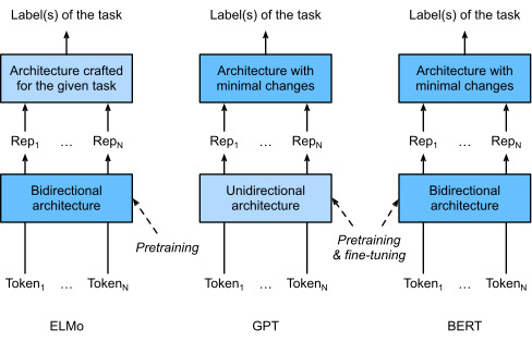
 

Fig. 15.8.1  A comparison of ELMo, GPT, and BERT.


BERT further improved the state of the art on eleven natural language processing tasks under broad categories of (i) single text classification (e.g., sentiment analysis), (ii) text pair classification (e.g., natural language inference), (iii) question answering, (iv) text tagging (e.g., named entity recognition). All proposed in 2018, from context-sensitive ELMo to task-agnostic GPT and BERT, conceptually simple yet empirically powerful pretraining of deep representations for natural languages have revolutionized solutions to various natural language processing tasks.


BERT는 (i) 단일 텍스트 분류(예: 감정 분석), (ii) 텍스트 쌍 분류(예: 자연어 추론), (iii) 질문 응답의 광범위한 범주에서 11가지 자연어 처리 작업에 대한 최신 기술을 더욱 개선했습니다. , (iv) 텍스트 태깅(예: 명명된 개체 인식). context-sensitive ELMo부터 task-agnostic GPT 및 BERT에 이르기까지 2018년에 제안된 모든 것, 개념적으로 단순하지만 경험적으로 강력한 자연어에 대한 심층 표현 사전 학습은 다양한 자연어 처리 작업에 대한 솔루션에 혁명을 일으켰습니다.


In the rest of this chapter, we will dive into the pretraining of BERT. When natural language processing applications are explained in Section 16, we will illustrate fine-tuning of BERT for downstream applications.


이 장의 나머지 부분에서는 BERT의 사전 훈련에 대해 살펴보겠습니다. 섹션 16에서 자연어 처리 애플리케이션을 설명할 때 다운스트림 애플리케이션을 위한 BERT의 미세 조정을 설명합니다.


import torch
from torch import nn
from d2l import torch as d2l


15.8.4. Input Representation


In natural language processing, some tasks (e.g., sentiment analysis) take single text as input, while in some other tasks (e.g., natural language inference), the input is a pair of text sequences. The BERT input sequence unambiguously represents both single text and text pairs. In the former, the BERT input sequence is the concatenation of the special classification token “<cls>”, tokens of a text sequence, and the special separation token “<sep>”. In the latter, the BERT input sequence is the concatenation of “<cls>”, tokens of the first text sequence, “<sep>”, tokens of the second text sequence, and “<sep>”. We will consistently distinguish the terminology “BERT input sequence” from other types of “sequences”. For instance, one BERT input sequence may include either one text sequence or two text sequences.


자연어 처리에서 일부 작업(예: 감정 분석)은 단일 텍스트를 입력으로 사용하는 반면, 일부 다른 작업(예: 자연어 추론)에서는 입력이 텍스트 시퀀스 쌍입니다. BERT 입력 시퀀스는 단일 텍스트와 텍스트 쌍을 모두 명확하게 나타냅니다. 전자의 경우 BERT 입력 시퀀스는 특수 분류 토큰 “<cls>”, 텍스트 시퀀스 토큰 및 특수 분리 토큰 “<sep>”의 연결입니다. 후자의 경우, BERT 입력 시퀀스는 첫 번째 텍스트 시퀀스의 토큰인 "<cls>", 두 번째 텍스트 시퀀스의 토큰인 "<sep>" 및 "<sep>"의 연결입니다. 우리는 "BERT 입력 시퀀스"라는 용어를 다른 유형의 "시퀀스"와 일관되게 구별할 것입니다. 예를 들어, 하나의 BERT 입력 시퀀스에는 하나의 텍스트 시퀀스 또는 두 개의 텍스트 시퀀스가 포함될 수 있습니다.
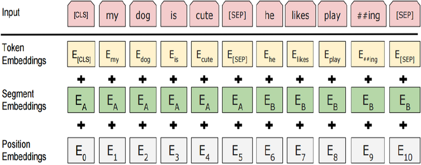
 

To distinguish text pairs, the learned segment embeddings eA and eB are added to the token embeddings of the first sequence and the second sequence, respectively. For single text inputs, only eA is used.


텍스트 쌍을 구별하기 위해 학습된 세그먼트 임베딩 eA 및 eB가 각각 첫 번째 시퀀스와 두 번째 시퀀스의 토큰 임베딩에 추가됩니다. 단일 텍스트 입력의 경우 eA만 사용됩니다.


The following get_tokens_and_segments takes either one sentence or two sentences as input, then returns tokens of the BERT input sequence and their corresponding segment IDs.


다음 get_tokens_and_segments는 한 문장 또는 두 문장을 입력으로 사용한 다음 BERT 입력 시퀀스의 토큰과 해당 세그먼트 ID를 반환합니다.


#@save
def get_tokens_and_segments(tokens_a, tokens_b=None):
    """Get tokens of the BERT input sequence and their segment IDs."""
    tokens = ['<cls>'] + tokens_a + ['<sep>']
    # 0 and 1 are marking segment A and B, respectively
    segments = [0] * (len(tokens_a) + 2)
    if tokens_b is not None:
        tokens += tokens_b + ['<sep>']
        segments += [1] * (len(tokens_b) + 1)
    return tokens, segments

이 함수는 BERT 모델의 입력으로 사용되는 토큰과 세그먼트 ID를 생성하는 과정을 수행합니다. BERT의 입력 형식은 [CLS] - 토큰 A - [SEP] - 토큰 B - [SEP]으로 구성되며, 이때 세그먼트 A는 토큰 A에 대한 세그먼트 ID(0), 세그먼트 B는 토큰 B에 대한 세그먼트 ID(1)를 나타냅니다.

  1. tokens_a: 첫 번째 시퀀스의 토큰 리스트입니다.
  2. tokens_b: 두 번째 시퀀스의 토큰 리스트(선택 사항)입니다.

함수 내용:

  • tokens: BERT 입력 시퀀스에 해당하는 토큰 리스트를 구성합니다. 시퀀스의 처음은 [CLS] 토큰으로 시작하고, 첫 번째 시퀀스의 토큰들을 이어붙인 후 [SEP] 토큰을 추가합니다. 두 번째 시퀀스가 제공되면 해당 시퀀스의 토큰들을 이어붙이고 다시 [SEP] 토큰을 추가합니다.
  • segments: 각 토큰의 세그먼트 ID를 나타내는 리스트를 구성합니다. 세그먼트 A는 토큰 A에 대한 것이므로 길이는 tokens_a의 길이 + 2입니다. 만약 두 번째 시퀀스가 제공되면 해당 시퀀스에 대한 세그먼트 ID를 추가합니다.

이 함수를 통해 토큰과 세그먼트 ID를 생성하여 BERT 입력 형식에 맞게 구성할 수 있습니다.


BERT chooses the Transformer encoder as its bidirectional architecture. Common in the Transformer encoder, positional embeddings are added at every position of the BERT input sequence. However, different from the original Transformer encoder, BERT uses learnable positional embeddings. To sum up, Fig. 15.8.2 shows that the embeddings of the BERT input sequence are the sum of the token embeddings, segment embeddings, and positional embeddings.


15.8. Bidirectional Encoder Representations from Transformers (BERT) — Dive into Deep Learning 1.0.3 documentation


d2l.ai

BERT는 양방향 아키텍처로 Transformer 인코더를 선택합니다. Transformer 인코더에서 일반적으로 위치 임베딩은 BERT 입력 시퀀스의 모든 위치에 추가됩니다. 그러나 원래 Transformer 인코더와 달리 BERT는 학습 가능한 위치 임베딩을 사용합니다. 요약하면 그림 15.8.2는 BERT 입력 시퀀스의 임베딩이 토큰 임베딩, 세그먼트 임베딩 및 위치 임베딩의 합임을 보여줍니다.
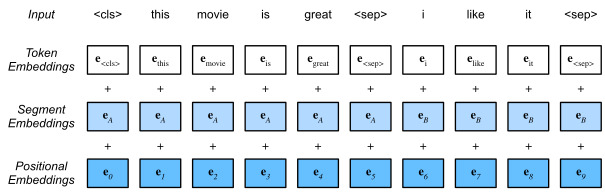
 

Fig. 15.8.2&nbsp; The embeddings of the BERT input sequence are the sum of the token embeddings, segment embeddings, and positional embeddings.


The following BERTEncoder class is similar to the TransformerEncoder class as implemented in Section 11.7. Different from TransformerEncoder, BERTEncoder uses segment embeddings and learnable positional embeddings.


다음 BERTEncoder 클래스는 섹션 11.7에 구현된 TransformerEncoder 클래스와 유사합니다. TransformerEncoder와 달리 BERTEncoder는 세그먼트 임베딩과 학습 가능한 위치 임베딩을 사용합니다.


#@save
class BERTEncoder(nn.Module):
    """BERT encoder."""
    def __init__(self, vocab_size, num_hiddens, ffn_num_hiddens, num_heads,
                 num_blks, dropout, max_len=1000, **kwargs):
        super(BERTEncoder, self).__init__(**kwargs)
        self.token_embedding = nn.Embedding(vocab_size, num_hiddens)
        self.segment_embedding = nn.Embedding(2, num_hiddens)
        self.blks = nn.Sequential()
        for i in range(num_blks):
            self.blks.add_module(f"{i}", d2l.TransformerEncoderBlock(
                num_hiddens, ffn_num_hiddens, num_heads, dropout, True))
        # In BERT, positional embeddings are learnable, thus we create a
        # parameter of positional embeddings that are long enough
        self.pos_embedding = nn.Parameter(torch.randn(1, max_len,
                                                      num_hiddens))

    def forward(self, tokens, segments, valid_lens):
        # Shape of `X` remains unchanged in the following code snippet:
        # (batch size, max sequence length, `num_hiddens`)
        X = self.token_embedding(tokens) + self.segment_embedding(segments)
        X = X + self.pos_embedding[:, :X.shape[1], :]
        for blk in self.blks:
            X = blk(X, valid_lens)
        return X

이 클래스는 BERT 모델의 인코더 부분을 정의합니다. BERT 모델은 토큰 임베딩, 세그먼트 임베딩, 여러 개의 변환기 블록 및 위치 임베딩을 포함하고 있습니다.

  • vocab_size: 토큰의 종류 수입니다.
  • num_hiddens: 임베딩 차원 및 히든 레이어의 차원입니다.
  • ffn_num_hiddens: Feed-Forward 신경망의 히든 레이어 차원입니다.
  • num_heads: Multi-Head Attention의 헤드 수입니다.
  • num_blks: 변환기 블록의 개수입니다.
  • dropout: 드롭아웃 비율입니다.
  • max_len: 최대 시퀀스 길이입니다.
  • kwargs: 추가 매개변수입니다.

이 클래스는 다음과 같은 요소들로 구성됩니다:

  • token_embedding: 토큰 임베딩 레이어입니다. 입력 토큰을 임베딩 벡터로 변환합니다.
  • segment_embedding: 세그먼트 임베딩 레이어입니다. 입력 세그먼트 정보를 임베딩 벡터로 변환합니다.
  • blks: 여러 개의 변환기 블록을 포함하는 순차적인 레이어입니다.
  • pos_embedding: 위치 임베딩 매개변수로서, BERT에서 위치 임베딩은 학습 가능합니다.

forward 메서드에서는 다음과 같은 작업을 수행합니다:

  1. token_embedding과 segment_embedding을 사용하여 토큰과 세그먼트 임베딩을 생성합니다.
  2. 위치 임베딩을 추가합니다.
  3. blks에 있는 각 변환기 블록을 차례로 통과시킵니다.
  4. 최종 인코딩 결과를 반환합니다.

이를 통해 BERTEncoder 클래스는 BERT의 인코더 부분을 구현하며, 입력 토큰과 세그먼트를 받아서 인코딩된 벡터를 반환합니다.


Suppose that the vocabulary size is 10000. To demonstrate forward inference of BERTEncoder, let’s create an instance of it and initialize its parameters.


어휘 크기가 10000이라고 가정합니다. BERTEncoder의 순방향 추론을 시연하기 위해 인스턴스를 만들고 해당 매개변수를 초기화하겠습니다.


vocab_size, num_hiddens, ffn_num_hiddens, num_heads = 10000, 768, 1024, 4
ffn_num_input, num_blks, dropout = 768, 2, 0.2
encoder = BERTEncoder(vocab_size, num_hiddens, ffn_num_hiddens, num_heads,
                      num_blks, dropout)

위의 코드에서 다음과 같은 변수들을 설정하고 있습니다:

  • vocab_size: 어휘 크기로, 모델에서 다루는 토큰의 종류 수입니다.
  • num_hiddens: 임베딩 차원 및 각 변환기 블록의 출력 차원입니다.
  • ffn_num_hiddens: Feed-Forward 신경망의 히든 레이어 차원입니다.
  • num_heads: Multi-Head Attention의 헤드 수입니다.
  • ffn_num_input: Feed-Forward 신경망의 입력 차원으로, 일반적으로 num_hiddens와 동일합니다.
  • num_blks: 변환기 블록의 개수입니다.
  • dropout: 드롭아웃 비율입니다.

그리고 BERTEncoder 클래스의 인스턴스인 encoder를 생성합니다. 이를 통해 BERT 인코더 모델을 정의하고 인코딩 작업을 수행할 수 있게 됩니다. encoder 객체는 위에서 설정한 매개변수들을 바탕으로 BERT 인코더를 생성한 것입니다.


We define tokens to be 2 BERT input sequences of length 8, where each token is an index of the vocabulary. The forward inference of BERTEncoder with the input tokens returns the encoded result where each token is represented by a vector whose length is predefined by the hyperparameter num_hiddens. This hyperparameter is usually referred to as the hidden size (number of hidden units) of the Transformer encoder.


우리는 토큰을 길이 8의 2개의 BERT 입력 시퀀스로 정의합니다. 여기서 각 토큰은 어휘의 인덱스입니다. 입력 토큰을 사용한 BERTEncoder의 순방향 추론은 각 토큰이 하이퍼파라미터 num_hiddens에 의해 길이가 미리 정의된 벡터로 표현되는 인코딩된 결과를 반환합니다. 이 하이퍼파라미터는 일반적으로 Transformer 인코더의 숨겨진 크기(숨겨진 단위 수)라고 합니다.


tokens = torch.randint(0, vocab_size, (2, 8))
segments = torch.tensor([[0, 0, 0, 0, 1, 1, 1, 1], [0, 0, 0, 1, 1, 1, 1, 1]])
encoded_X = encoder(tokens, segments, None)
encoded_X.shape

위 코드에서 다음과 같은 작업을 수행하고 있습니다:

  1. tokens와 segments 생성: 임의의 정수로 구성된 tokens와 세그먼트 정보를 생성합니다. tokens는 (2, 8) 모양의 텐서로, 2개의 시퀀스 각각에 8개의 토큰이 포함되어 있습니다. segments는 (2, 8) 모양의 텐서로, 세그먼트 정보를 나타내는데 0은 첫 번째 세그먼트를, 1은 두 번째 세그먼트를 나타냅니다.
  2. 인코딩: encoder 객체를 사용하여 tokens와 segments를 인코딩한 결과를 계산합니다. 이를 encoded_X에 저장합니다. 이 과정은 BERT 인코더의 forward 연산과정을 의미합니다. 입력 토큰과 세그먼트 정보를 통해 인코딩된 특성 행렬을 얻게 됩니다.
  3. 결과 확인: encoded_X의 형태(shape)를 출력하여 인코딩된 결과의 텐서 모양을 확인합니다. 출력된 형태는 인코딩된 특성 행렬의 모양을 나타냅니다.

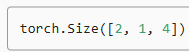
결과적으로 encoded_X는 인코딩된 특성 행렬로, 첫 번째 차원은 시퀀스의 개수, 두 번째 차원은 시퀀스의 길이, 세 번째 차원은 임베딩 차원(num_hiddens)으로 구성됩니다. 따라서 encoded_X.shape의 결과는 (2, 8, 768)이 됩니다.

torch.Size([2, 8, 768])


15.8.5. Pretraining Tasks


The forward inference of BERTEncoder gives the BERT representation of each token of the input text and the inserted special tokens “<cls>” and “<seq>”. Next, we will use these representations to compute the loss function for pretraining BERT. The pretraining is composed of the following two tasks: masked language modeling and next sentence prediction.


BERTEncoder의 순방향 추론은 입력 텍스트의 각 토큰과 삽입된 특수 토큰 "<cls>" 및 "<seq>"에 대한 BERT representation을 제공합니다. 다음으로 이러한 representations을 사용하여 BERT 사전 학습을 위한 손실 함수를 계산합니다. 사전 훈련은 마스크된 언어 모델링과 다음 문장 예측이라는 두 가지 작업으로 구성됩니다.


15.8.5.1. Masked Language Modeling

As illustrated in Section 9.3, a language model predicts a token using the context on its left. To encode context bidirectionally for representing each token, BERT randomly masks tokens and uses tokens from the bidirectional context to predict the masked tokens in a self-supervised fashion. This task is referred to as a masked language model.


섹션 9.3에 설명된 대로 언어 모델은 왼쪽의 컨텍스트를 사용하여 토큰을 예측합니다. 각 토큰을 표현하기 위해 컨텍스트를 양방향으로 인코딩하기 위해 BERT는 토큰을 무작위로 마스킹하고 양방향 컨텍스트의 토큰을 사용하여 자체 감독 방식으로 마스킹된 토큰을 예측합니다. 이 작업을 마스크된 언어 모델이라고 합니다.


In this pretraining task, 15% of tokens will be selected at random as the masked tokens for prediction. To predict a masked token without cheating by using the label, one straightforward approach is to always replace it with a special “<mask>” token in the BERT input sequence. However, the artificial special token “<mask>” will never appear in fine-tuning. To avoid such a mismatch between pretraining and fine-tuning, if a token is masked for prediction (e.g., “great” is selected to be masked and predicted in “this movie is great”), in the input it will be replaced with:


이 사전 훈련 작업에서는 토큰의 15%가 예측을 위한 마스크된 토큰으로 무작위로 선택됩니다. 레이블을 사용하여 부정 행위 없이 마스킹된 토큰을 예측하기 위한 한 가지 간단한 접근 방식은 항상 BERT 입력 시퀀스에서 특수 "<mask>" 토큰으로 바꾸는 것입니다. 그러나 인공 특수 토큰 “<mask>”는 미세 조정에서는 절대 나타나지 않습니다. 사전 훈련과 미세 조정 사이의 불일치를 피하기 위해 토큰이 예측을 위해 마스크된 경우(예: "이 영화는 훌륭합니다"에서 "훌륭함"이 마스크되고 예측되도록 선택됨) 입력에서 다음으로 대체됩니다.


  • a special “<mask>” token for 80% of the time (e.g., “this movie is great” becomes “this movie is <mask>”);

    80%의 시간 동안 특수 "<마스크>" 토큰(예: "이 영화는 훌륭합니다"는 "이 영화는 <마스크>입니다"가 됨)

  • a random token for 10% of the time (e.g., “this movie is great” becomes “this movie is drink”);

    10%의 시간에 대한 무작위 토큰(예: "이 영화는 훌륭해요"는 "이 영화는 술입니다"가 됩니다)

  • the unchanged label token for 10% of the time (e.g., “this movie is great” becomes “this movie is great”).

    10%의 시간 동안 변경되지 않은 레이블 토큰(예: "이 영화는 훌륭합니다"는 "이 영화는 훌륭합니다"가 됨)


Note that for 10% of 15% time a random token is inserted. This occasional noise encourages BERT to be less biased towards the masked token (especially when the label token remains unchanged) in its bidirectional context encoding.


15% 시간 중 10% 동안 무작위 토큰이 삽입된다는 점에 유의하세요. 이러한 간헐적인 노이즈는 BERT가 양방향 컨텍스트 인코딩에서 마스크된 토큰(특히 레이블 토큰이 변경되지 않은 상태로 유지되는 경우)에 덜 편향되도록 장려합니다.


We implement the following MaskLM class to predict masked tokens in the masked language model task of BERT pretraining. The prediction uses a one-hidden-layer MLP (self.mlp). In forward inference, it takes two inputs: the encoded result of BERTEncoder and the token positions for prediction. The output is the prediction results at these positions.


BERT 사전 학습의 마스크된 언어 모델 작업에서 마스크된 토큰을 예측하기 위해 다음 MaskLM 클래스를 구현합니다. 예측은 단일 숨겨진 레이어 MLP(self.mlp)를 사용합니다. 순방향 추론에서는 BERTEncoder의 인코딩된 결과와 예측을 위한 토큰 위치라는 두 가지 입력을 사용합니다. 출력은 이러한 위치에서의 예측 결과입니다.


#@save
class MaskLM(nn.Module):
    """The masked language model task of BERT."""
    def __init__(self, vocab_size, num_hiddens, **kwargs):
        super(MaskLM, self).__init__(**kwargs)
        self.mlp = nn.Sequential(nn.LazyLinear(num_hiddens),
                                 nn.ReLU(),
                                 nn.LayerNorm(num_hiddens),
                                 nn.LazyLinear(vocab_size))

    def forward(self, X, pred_positions):
        num_pred_positions = pred_positions.shape[1]
        pred_positions = pred_positions.reshape(-1)
        batch_size = X.shape[0]
        batch_idx = torch.arange(0, batch_size)
        # Suppose that `batch_size` = 2, `num_pred_positions` = 3, then
        # `batch_idx` is `torch.tensor([0, 0, 0, 1, 1, 1])`
        batch_idx = torch.repeat_interleave(batch_idx, num_pred_positions)
        masked_X = X[batch_idx, pred_positions]
        masked_X = masked_X.reshape((batch_size, num_pred_positions, -1))
        mlm_Y_hat = self.mlp(masked_X)
        return mlm_Y_hat

위의 코드에서 수행되는 작업은 다음과 같습니다:

  1. 초기화 메서드(__init__): MaskLM 클래스의 초기화 메서드에서는 MLM 작업을 위한 신경망 구조를 정의합니다. num_hiddens는 은닉 유닛의 수, vocab_size는 어휘 크기를 나타냅니다.
  2. Forward 메서드(forward): 이 메서드는 BERT의 마스킹된 언어 모델 작업을 수행합니다. 입력으로 주어진 X는 BERT 인코더의 출력입니다. pred_positions는 마스킹된 위치를 나타내는 텐서로, 예측해야 할 위치에 대한 정보를 가지고 있습니다.
    • pred_positions의 형태(shape)를 조정하여 마스크된 위치 정보를 준비합니다.
    • 마스크된 위치에 해당하는 특성만 추출하여 masked_X를 생성합니다.
    • masked_X를 MLP 모델(self.mlp)에 통과시켜 마스킹된 언어 모델의 예측값을 계산합니다.

즉, 이 모듈은 인코더의 출력을 받아서 마스크된 위치의 특성을 추출하고, 이를 통해 마스킹된 언어 모델 작업을 수행하여 단어 예측을 수행합니다.


To demonstrate the forward inference of MaskLM, we create its instance mlm and initialize it. Recall that encoded_X from the forward inference of BERTEncoder represents 2 BERT input sequences. We define mlm_positions as the 3 indices to predict in either BERT input sequence of encoded_X. The forward inference of mlm returns prediction results mlm_Y_hat at all the masked positions mlm_positions of encoded_X. For each prediction, the size of the result is equal to the vocabulary size.


MaskLM의 순방향 추론을 보여주기 위해 인스턴스 mlm을 생성하고 초기화합니다. BERTEncoder의 순방향 추론에서 나온 Encoded_X는 2개의 BERT 입력 시퀀스를 나타냅니다. 우리는 mlm_positions를 Encoded_X의 BERT 입력 시퀀스에서 예측할 3개의 인덱스로 정의합니다. mlm의 순방향 추론은 Encoded_X의 모든 마스크 위치 mlm_positions에서 예측 결과 mlm_Y_hat를 반환합니다. 각 예측에 대해 결과의 크기는 어휘 크기와 같습니다.


mlm = MaskLM(vocab_size, num_hiddens)
mlm_positions = torch.tensor([[1, 5, 2], [6, 1, 5]])
mlm_Y_hat = mlm(encoded_X, mlm_positions)
mlm_Y_hat.shape

위의 코드에서 수행되는 작업은 다음과 같습니다:

  1. MaskLM 모델 생성: MaskLM 클래스로부터 MLM 모델을 생성합니다. vocab_size는 어휘 크기, num_hiddens는 은닉 유닛의 수입니다.
  2. 마스크된 위치 정보 생성: mlm_positions 텐서는 마스킹된 위치 정보를 나타내며, 이 정보를 통해 모델은 어떤 위치의 단어를 예측할지 결정합니다.
  3. MLM 모델 적용: 생성한 mlm 모델에 인코딩된 입력 encoded_X와 마스크된 위치 정보 mlm_positions를 전달하여 마스킹된 언어 모델 작업을 수행합니다. 모델은 이 위치에서 어떤 단어가 들어갈지 예측한 결과를 반환합니다.
  4. 결과 확인: mlm_Y_hat은 마스킹된 언어 모델의 예측 결과입니다. 이 결과의 형태(shape)를 확인하면 마스크된 위치의 단어 예측에 대한 확률값 분포를 확인할 수 있습니다.

즉, 위의 코드는 MaskLM 모델을 사용하여 BERT의 마스킹된 언어 모델 작업을 수행하고, 예측 결과의 형태(shape)를 출력하는 예제입니다

torch.Size([6])


15.8.5.2. Next Sentence Prediction


Although masked language modeling is able to encode bidirectional context for representing words, it does not explicitly model the logical relationship between text pairs. To help understand the relationship between two text sequences, BERT considers a binary classification task, next sentence prediction, in its pretraining. When generating sentence pairs for pretraining, for half of the time they are indeed consecutive sentences with the label “True”; while for the other half of the time the second sentence is randomly sampled from the corpus with the label “False”.


마스킹된 언어 모델링은 단어를 표현하기 위해 양방향 컨텍스트를 인코딩할 수 있지만 텍스트 쌍 간의 논리적 관계를 명시적으로 모델링하지는 않습니다. 두 텍스트 시퀀스 간의 관계를 이해하는 데 도움을 주기 위해 BERT는 사전 학습에서 이진 분류 작업, 다음 문장 예측을 고려합니다. 사전 학습을 위해 문장 쌍을 생성할 때 절반의 시간 동안 실제로는 "True"라는 레이블이 붙은 연속 문장입니다. 나머지 절반 동안은 "False"라는 라벨이 붙은 코퍼스에서 두 번째 문장이 무작위로 샘플링됩니다.


The following NextSentencePred class uses a one-hidden-layer MLP to predict whether the second sentence is the next sentence of the first in the BERT input sequence. Due to self-attention in the Transformer encoder, the BERT representation of the special token “<cls>” encodes both the two sentences from the input. Hence, the output layer (self.output) of the MLP classifier takes X as input, where X is the output of the MLP hidden layer whose input is the encoded “<cls>” token.


다음 NextSentencePred 클래스는 단일 숨겨진 레이어 MLP를 사용하여 두 번째 문장이 BERT 입력 시퀀스에서 첫 번째 문장의 다음 문장인지 예측합니다. Transformer 인코더의 self-attention으로 인해 특수 토큰 “<cls>”의 BERT 표현은 입력의 두 문장을 모두 인코딩합니다. 따라서 MLP 분류기의 출력 계층(self.output)은 X를 입력으로 사용합니다. 여기서 X는 입력이 인코딩된 "<cls>" 토큰인 MLP 숨겨진 계층의 출력입니다.


#@save
class NextSentencePred(nn.Module):
    """The next sentence prediction task of BERT."""
    def __init__(self, **kwargs):
        super(NextSentencePred, self).__init__(**kwargs)
        self.output = nn.LazyLinear(2)

    def forward(self, X):
        # `X` shape: (batch size, `num_hiddens`)
        return self.output(X)

위의 코드에서 수행되는 작업은 다음과 같습니다:

  1. NextSentencePred 모듈 생성: NextSentencePred 클래스로부터 다음 문장 예측 작업을 수행하는 모듈을 생성합니다.
  2. 모듈 구성: 모듈 내부에는 출력을 생성하는 레이어인 nn.LazyLinear이 정의되어 있습니다. nn.LazyLinear(2)는 출력 레이어를 생성하며, 이 레이어는 2개의 출력 유닛을 가집니다. 이것은 다음 문장이 관련성이 있을지 없을지에 대한 이진 예측을 수행하기 위한 레이어입니다.
  3. Forward 연산: forward 함수는 주어진 입력 X를 받아 출력을 계산합니다. X의 형태는 (배치 크기, num_hiddens)입니다. 입력 X를 출력 레이어에 전달하여 다음 문장 예측 작업을 수행하고 결과를 반환합니다.

위의 코드는 BERT의 다음 문장 예측 작업을 위한 모듈인 NextSentencePred를 정의하는 예제입니다.


We can see that the forward inference of an NextSentencePred instance returns binary predictions for each BERT input sequence.


NextSentencePred 인스턴스의 순방향 추론이 각 BERT 입력 시퀀스에 대해 이진 예측을 반환하는 것을 볼 수 있습니다.


# PyTorch by default will not flatten the tensor as seen in mxnet where, if
# flatten=True, all but the first axis of input data are collapsed together
encoded_X = torch.flatten(encoded_X, start_dim=1)
# input_shape for NSP: (batch size, `num_hiddens`)
nsp = NextSentencePred()
nsp_Y_hat = nsp(encoded_X)
nsp_Y_hat.shape

위의 코드에서 수행되는 작업은 다음과 같습니다:

  1. encoded_X 펼치기: torch.flatten 함수를 사용하여 encoded_X 텐서를 펼치는 작업을 수행합니다. encoded_X는 이전 단계에서 인코딩된 BERT 출력 텐서로, 차원을 펼쳐서 2차원으로 만듭니다. start_dim=1 인자는 펼치는 시작 차원을 지정합니다.
  2. NextSentencePred 모듈 생성: 다음 문장 예측 작업을 위한 NextSentencePred 모듈을 생성합니다.
  3. Forward 연산: 생성된 NextSentencePred 모듈에 펼쳐진 encoded_X를 입력으로 전달하여 다음 문장 예측 작업을 수행하고, 결과 nsp_Y_hat을 얻습니다.
  4. 결과 확인: nsp_Y_hat의 형태(shape)를 확인하여 다음 문장 예측 작업의 결과를 파악합니다. 결과 형태는 (batch size, 2)입니다. 두 개의 출력 유닛은 각각 두 가지 다른 클래스(다음 문장이 관련성이 있을 경우 1, 없을 경우 0)에 대한 확률 예측을 나타냅니다.

위의 코드는 BERT의 다음 문장 예측 작업을 수행하는 예제로, 인코딩된 텍스트 데이터를 입력으로 하여 다음 문장이 관련성이 있을지 없을지를 예측하는 모듈을 생성하고 결과를 확인하는 과정을 보여줍니다

torch.Size([2, 2])

The cross-entropy loss of the 2 binary classifications can also be computed.


2개의 이진 분류의 교차 엔트로피 손실도 계산할 수 있습니다.


nsp_y = torch.tensor([0, 1])
nsp_l = loss(nsp_Y_hat, nsp_y)
nsp_l.shape

위의 코드에서 수행되는 작업은 다음과 같습니다:

  1. nsp_y 정의: 다음 문장 예측 작업에서 실제 정답 레이블을 나타내는 텐서 nsp_y를 정의합니다. 이 예제에서는 두 개의 미니배치 샘플에 대한 정답 레이블을 나타냅니다. 첫 번째 샘플은 관련성이 없는 경우(0), 두 번째 샘플은 관련성이 있는 경우(1)를 나타냅니다.
  2. 손실 계산: 앞서 정의한 nsp_Y_hat 텐서와 nsp_y 정답 레이블을 사용하여 다음 문장 예측 작업의 손실을 계산합니다. 이를 위해 사용하는 손실 함수인 loss는 코드에는 나타나지 않았지만, BERT의 다음 문장 예측 작업에서는 일반적으로 교차 엔트로피(Cross Entropy) 손실이 사용됩니다.
  3. 손실 형태 확인: nsp_l의 형태(shape)를 확인하여 계산된 손실의 형태를 파악합니다. 이 경우 nsp_l은 스칼라값입니다. 미니배치 내 각 샘플에 대한 손실을 합한 결과를 나타냅니다.

위의 코드는 BERT의 다음 문장 예측 작업에서 손실을 계산하는 과정을 보여주는 예제입니다.

torch.Size([2])


It is noteworthy that all the labels in both the aforementioned pretraining tasks can be trivially obtained from the pretraining corpus without manual labeling effort. The original BERT has been pretrained on the concatenation of BookCorpus (Zhu et al., 2015) and English Wikipedia. These two text corpora are huge: they have 800 million words and 2.5 billion words, respectively.


앞서 언급한 사전 훈련 작업의 모든 레이블은 수동 레이블 지정 작업 없이 사전 훈련 코퍼스에서 쉽게 얻을 수 있다는 점은 주목할 만합니다. 원래 BERT는 BookCorpus(Zhu et al., 2015)와 English Wikipedia의 연결을 통해 사전 학습되었습니다. 이 두 개의 텍스트 말뭉치에는 각각 8억 단어와 25억 단어가 있습니다.


15.8.6. Putting It All Together

When pretraining BERT, the final loss function is a linear combination of both the loss functions for masked language modeling and next sentence prediction. Now we can define the BERTModel class by instantiating the three classes BERTEncoder, MaskLM, and NextSentencePred. The forward inference returns the encoded BERT representations encoded_X, predictions of masked language modeling mlm_Y_hat, and next sentence predictions nsp_Y_hat.


BERT를 사전 훈련할 때 최종 손실 함수는 마스크된 언어 모델링과 다음 문장 예측을 위한 손실 함수의 선형 조합입니다. 이제 BERTEncoder, MaskLM 및 NextSentencePred 세 클래스를 인스턴스화하여 BERTModel 클래스를 정의할 수 있습니다. 순방향 추론은 인코딩된 BERT 표현 encode_X, 마스크된 언어 모델링 mlm_Y_hat의 예측 및 다음 문장 예측 nsp_Y_hat을 반환합니다.


#@save
class BERTModel(nn.Module):
    """The BERT model."""
    def __init__(self, vocab_size, num_hiddens, ffn_num_hiddens,
                 num_heads, num_blks, dropout, max_len=1000):
        super(BERTModel, self).__init__()
        self.encoder = BERTEncoder(vocab_size, num_hiddens, ffn_num_hiddens,
                                   num_heads, num_blks, dropout,
                                   max_len=max_len)
        self.hidden = nn.Sequential(nn.LazyLinear(num_hiddens),
                                    nn.Tanh())
        self.mlm = MaskLM(vocab_size, num_hiddens)
        self.nsp = NextSentencePred()

    def forward(self, tokens, segments, valid_lens=None, pred_positions=None):
        encoded_X = self.encoder(tokens, segments, valid_lens)
        if pred_positions is not None:
            mlm_Y_hat = self.mlm(encoded_X, pred_positions)
        else:
            mlm_Y_hat = None
        # The hidden layer of the MLP classifier for next sentence prediction.
        # 0 is the index of the '<cls>' token
        nsp_Y_hat = self.nsp(self.hidden(encoded_X[:, 0, :]))
        return encoded_X, mlm_Y_hat, nsp_Y_hat

위의 코드에서 수행되는 작업은 다음과 같습니다:

  1. nsp_y 정의: 다음 문장 예측 작업에서 실제 정답 레이블을 나타내는 텐서 nsp_y를 정의합니다. 이 예제에서는 두 개의 미니배치 샘플에 대한 정답 레이블을 나타냅니다. 첫 번째 샘플은 관련성이 없는 경우(0), 두 번째 샘플은 관련성이 있는 경우(1)를 나타냅니다.
  2. 손실 계산: 앞서 정의한 nsp_Y_hat 텐서와 nsp_y 정답 레이블을 사용하여 다음 문장 예측 작업의 손실을 계산합니다. 이를 위해 사용하는 손실 함수인 loss는 코드에는 나타나지 않았지만, BERT의 다음 문장 예측 작업에서는 일반적으로 교차 엔트로피(Cross Entropy) 손실이 사용됩니다.
  3. 손실 형태 확인: nsp_l의 형태(shape)를 확인하여 계산된 손실의 형태를 파악합니다. 이 경우 nsp_l은 스칼라값입니다. 미니배치 내 각 샘플에 대한 손실을 합한 결과를 나타냅니다.

위의 코드는 BERT의 다음 문장 예측 작업에서 손실을 계산하는 과정을 보여주는 예제입니다.

15.8.7. Summary

  • Word embedding models such as word2vec and GloVe are context-independent. They assign the same pretrained vector to the same word regardless of the context of the word (if any). It is hard for them to handle well polysemy or complex semantics in natural languages.

    word2vec 및 GloVe와 같은 단어 임베딩 모델은 상황에 독립적입니다. 단어의 맥락(있는 경우)에 관계없이 동일한 사전 훈련된 벡터를 동일한 단어에 할당합니다. 자연어에서는 다의어나 복잡한 의미를 잘 다루기가 어렵습니다.

  • For context-sensitive word representations such as ELMo and GPT, representations of words depend on their contexts.

    ELMo 및 GPT와 같은 상황에 맞는 단어 표현의 경우 단어 표현은 해당 상황에 따라 달라집니다.

  • ELMo encodes context bidirectionally but uses task-specific architectures (however, it is practically non-trivial to craft a specific architecture for every natural language processing task); while GPT is task-agnostic but encodes context left-to-right.

    ELMo는 컨텍스트를 양방향으로 인코딩하지만 작업별 아키텍처를 사용합니다(그러나 모든 자연어 처리 작업에 대해 특정 아키텍처를 만드는 것은 사실상 쉽지 않습니다). GPT는 작업에 구애받지 않지만 컨텍스트를 왼쪽에서 오른쪽으로 인코딩합니다.

  • BERT combines the best of both worlds: it encodes context bidirectionally and requires minimal architecture changes for a wide range of natural language processing tasks.

    BERT는 두 가지 장점을 결합합니다. 즉, 컨텍스트를 양방향으로 인코딩하고 광범위한 자연어 처리 작업에 대해 최소한의 아키텍처 변경이 필요합니다.

  • The embeddings of the BERT input sequence are the sum of the token embeddings, segment embeddings, and positional embeddings.

    BERT 입력 시퀀스의 임베딩은 토큰 임베딩, 세그먼트 임베딩 및 위치 임베딩의 합계입니다.

  • Pretraining BERT is composed of two tasks: masked language modeling and next sentence prediction. The former is able to encode bidirectional context for representing words, while the latter explicitly models the logical relationship between text pairs.

    사전 훈련 BERT는 마스크된 언어 모델링과 다음 문장 예측이라는 두 가지 작업으로 구성됩니다. 전자는 단어를 표현하기 위해 양방향 컨텍스트를 인코딩할 수 있는 반면, 후자는 텍스트 쌍 간의 논리적 관계를 명시적으로 모델링합니다.

https://www.youtube.com/live/QCOT5D7Pa7s?si=BfY_2QMLWpFqvm9T 

15.8.8. Exercises

  1. All other things being equal, will a masked language model require more or fewer pretraining steps to converge than a left-to-right language model? Why?
  2. In the original implementation of BERT, the positionwise feed-forward network in BERTEncoder (via d2l.TransformerEncoderBlock) and the fully connected layer in MaskLM both use the Gaussian error linear unit (GELU) (Hendrycks and Gimpel, 2016) as the activation function. Research into the difference between GELU and ReLU.


반응형


반응형

15.7. Word Similarity and Analogy — Dive into Deep Learning 1.0.3 documentation (d2l.ai)


15.7. Word Similarity and Analogy — Dive into Deep Learning 1.0.3 documentation


d2l.ai

15.7. Word Similarity and Analogy


In Section 15.4, we trained a word2vec model on a small dataset, and applied it to find semantically similar words for an input word. In practice, word vectors that are pretrained on large corpora can be applied to downstream natural language processing tasks, which will be covered later in Section 16. To demonstrate semantics of pretrained word vectors from large corpora in a straightforward way, let’s apply them in the word similarity and analogy tasks.


섹션 15.4에서는 작은 데이터 세트에 대해 word2vec 모델을 훈련하고 이를 적용하여 입력 단어에 대해 의미상 유사한 단어를 찾았습니다. 실제로 큰 말뭉치에서 사전 훈련된 단어 벡터는 다운스트림 자연어 처리 작업에 적용될 수 있으며 이에 대해서는 섹션 16에서 나중에 다룰 것입니다. 큰 말뭉치에서 사전 훈련된 단어 벡터의 의미를 간단한 방법으로 보여주기 위해 이것들을 유사성 및 비유 작업이라는 단어에 적용해 보겠습니다.


import os
import torch
from torch import nn
from d2l import torch as d2l


15.7.1. Loading Pretrained Word Vectors

Below lists pretrained GloVe embeddings of dimension 50, 100, and 300, which can be downloaded from the GloVe website. The pretrained fastText embeddings are available in multiple languages. Here we consider one English version (300-dimensional “wiki.en”) that can be downloaded from the fastText website.


아래에는 GloVe 웹사이트에서 다운로드할 수 있는 차원 50, 100, 300의 사전 훈련된 GloVe 임베딩이 나열되어 있습니다. 사전 훈련된 fastText 임베딩은 여러 언어로 제공됩니다. 여기에서는 fastText 웹사이트에서 다운로드할 수 있는 하나의 영어 버전(300차원 “wiki.en”)을 고려합니다.


#@save
d2l.DATA_HUB['glove.6b.50d'] = (d2l.DATA_URL + 'glove.6B.50d.zip',
                                '0b8703943ccdb6eb788e6f091b8946e82231bc4d')

#@save
d2l.DATA_HUB['glove.6b.100d'] = (d2l.DATA_URL + 'glove.6B.100d.zip',
                                 'cd43bfb07e44e6f27cbcc7bc9ae3d80284fdaf5a')

#@save
d2l.DATA_HUB['glove.42b.300d'] = (d2l.DATA_URL + 'glove.42B.300d.zip',
                                  'b5116e234e9eb9076672cfeabf5469f3eec904fa')

#@save
d2l.DATA_HUB['wiki.en'] = (d2l.DATA_URL + 'wiki.en.zip',
                           'c1816da3821ae9f43899be655002f6c723e91b88')

이 코드는 다양한 단어 임베딩 데이터셋에 대한 정보를 d2l.DATA_HUB 딕셔너리에 저장하는 역할을 합니다. 이 데이터셋들은 GloVe(글로브)와 위키백과 데이터의 영어 언어 버전입니다.

  1. d2l.DATA_HUB['glove.6b.50d']:
    • 'glove.6b.50d' 데이터셋의 정보를 저장합니다.
    • 데이터의 다운로드 경로와 해시값이 튜플로 저장됩니다.
  2. d2l.DATA_HUB['glove.6b.100d']:
    • 'glove.6b.100d' 데이터셋의 정보를 저장합니다.
  3. d2l.DATA_HUB['glove.42b.300d']:
    • 'glove.42b.300d' 데이터셋의 정보를 저장합니다.
  4. d2l.DATA_HUB['wiki.en']:
    • 'wiki.en' 데이터셋의 정보를 저장합니다.

이 코드는 데이터셋의 이름과 다운로드 경로, 해시값을 d2l.DATA_HUB 딕셔너리에 저장하여 데이터를 관리하는 데 사용됩니다.


To load these pretrained GloVe and fastText embeddings, we define the following TokenEmbedding class.


사전 학습된 GloVe 및 fastText 임베딩을 로드하기 위해 다음 TokenEmbedding 클래스를 정의합니다.


#@save
class TokenEmbedding:
    """Token Embedding."""
    def __init__(self, embedding_name):
        self.idx_to_token, self.idx_to_vec = self._load_embedding(
            embedding_name)
        self.unknown_idx = 0
        self.token_to_idx = {token: idx for idx, token in
                             enumerate(self.idx_to_token)}

    def _load_embedding(self, embedding_name):
        idx_to_token, idx_to_vec = ['<unk>'], []
        data_dir = d2l.download_extract(embedding_name)
        # GloVe website: https://nlp.stanford.edu/projects/glove/
        # fastText website: https://fasttext.cc/
        with open(os.path.join(data_dir, 'vec.txt'), 'r') as f:
            for line in f:
                elems = line.rstrip().split(' ')
                token, elems = elems[0], [float(elem) for elem in elems[1:]]
                # Skip header information, such as the top row in fastText
                if len(elems) > 1:
                    idx_to_token.append(token)
                    idx_to_vec.append(elems)
        idx_to_vec = [[0] * len(idx_to_vec[0])] + idx_to_vec
        return idx_to_token, torch.tensor(idx_to_vec)

    def __getitem__(self, tokens):
        indices = [self.token_to_idx.get(token, self.unknown_idx)
                   for token in tokens]
        vecs = self.idx_to_vec[torch.tensor(indices)]
        return vecs

    def __len__(self):
        return len(self.idx_to_token)

이 코드는 토큰 임베딩(Token Embedding)을 관리하는 TokenEmbedding 클래스를 정의합니다.

  1. class TokenEmbedding::
    • TokenEmbedding 클래스를 정의합니다.
  2. def __init__(self, embedding_name)::
    • 클래스의 초기화 함수입니다. embedding_name을 받아 해당 이름의 임베딩 데이터를 로드하고 초기화합니다.
    • idx_to_token, idx_to_vec, unknown_idx, token_to_idx 등의 속성을 초기화합니다.
  3. def _load_embedding(self, embedding_name)::
    • 임베딩 데이터를 로드하는 내부 함수입니다.
    • 주어진 embedding_name을 이용하여 해당 임베딩 데이터를 다운로드하고 읽어들입니다.
    • 임베딩 데이터의 내용을 idx_to_token, idx_to_vec 형태로 저장합니다.
  4. def __getitem__(self, tokens)::
    • 특정 토큰들에 대한 임베딩 벡터를 반환하는 함수입니다.
    • 토큰들을 인덱스로 변환한 후, 해당 인덱스에 해당하는 임베딩 벡터를 반환합니다.
  5. def __len__(self)::
    • 토큰의 개수를 반환하는 함수입니다.

이 클래스는 주어진 임베딩 데이터 이름에 따라 토큰 임베딩을 생성하고 관리하는 역할을 합니다.


Below we load the 50-dimensional GloVe embeddings (pretrained on a Wikipedia subset). When creating the TokenEmbedding instance, the specified embedding file has to be downloaded if it was not yet.


아래에서는 50차원 GloVe 임베딩(Wikipedia 하위 집합에서 사전 훈련됨)을 로드합니다. TokenEmbedding 인스턴스를 생성할 때 지정된 임베딩 파일이 아직 다운로드되지 않은 경우 다운로드해야 합니다.


glove_6b50d = TokenEmbedding('glove.6b.50d')

이 코드는 TokenEmbedding 클래스를 사용하여 'glove.6b.50d' 임베딩 데이터를 로드하고, glove_6b50d 객체를 생성하는 과정을 나타내고 있습니다.

  1. glove_6b50d = TokenEmbedding('glove.6b.50d'):
    • 'glove.6b.50d'라는 임베딩 데이터셋 이름을 가지고 TokenEmbedding 클래스의 객체 glove_6b50d를 생성합니다.
    • 이 객체는 'glove.6b.50d' 데이터셋의 토큰 임베딩을 관리하는 역할을 합니다.

이 코드는 'glove.6b.50d' 데이터셋의 토큰 임베딩을 TokenEmbedding 클래스를 사용하여 로드하고, 해당 임베딩을 관리하기 위한 객체를 생성하는 과정을 나타냅니다

Downloading ../data/glove.6B.50d.zip from http://d2l-data.s3-accelerate.amazonaws.com/glove.6B.50d.zip...


Output the vocabulary size. The vocabulary contains 400000 words (tokens) and a special unknown token.


어휘 크기를 출력합니다. 어휘에는 400,000개의 단어(토큰)와 특별한 알려지지 않은 토큰이 포함되어 있습니다.


len(glove_6b50d)
400001


We can get the index of a word in the vocabulary, and vice versa.


어휘에서 단어의 색인을 얻을 수 있고 그 반대의 경우도 마찬가지입니다.


glove_6b50d.token_to_idx['beautiful'], glove_6b50d.idx_to_token[3367]

이 코드는 'glove.6b.50d' 임베딩 데이터셋에서 'beautiful' 토큰의 인덱스와 인덱스 3367에 해당하는 토큰을 조회하는 과정을 나타내고 있습니다.

  1. glove_6b50d.token_to_idx['beautiful']:
    • 'beautiful' 토큰의 인덱스를 glove_6b50d 객체의 token_to_idx 속성을 사용하여 조회합니다.
    • 이 결과는 해당 토큰의 임베딩 벡터를 찾을 때 사용될 인덱스입니다.
  2. glove_6b50d.idx_to_token[3367]:
    • 인덱스 3367에 해당하는 토큰을 glove_6b50d 객체의 idx_to_token 속성을 사용하여 조회합니다.
    • 이 결과는 해당 인덱스가 어떤 토큰을 나타내는지를 알려줍니다.

이 코드는 'glove.6b.50d' 임베딩 데이터셋에서 'beautiful' 토큰의 인덱스를 조회하고, 인덱스 3367에 해당하는 토큰을 찾는 과정을 나타냅니다.

(3367, 'beautiful')


15.7.2. Applying Pretrained Word Vectors

Using the loaded GloVe vectors, we will demonstrate their semantics by applying them in the following word similarity and analogy tasks.


로드된 GloVe 벡터를 사용하여 다음 단어 유사성 및 유추 작업에 적용하여 의미를 보여줍니다.


15.7.2.1. Word Similarity

Similar to Section 15.4.3, in order to find semantically similar words for an input word based on cosine similarities between word vectors, we implement the following knn (k-nearest neighbors) function.


15.4.3절과 마찬가지로 단어 벡터 간의 코사인 유사성을 기반으로 입력 단어에 대해 의미상 유사한 단어를 찾기 위해 다음 knn(k-최근접 이웃) 함수를 구현합니다.


def knn(W, x, k):
    # Add 1e-9 for numerical stability
    cos = torch.mv(W, x.reshape(-1,)) / (
        torch.sqrt(torch.sum(W * W, axis=1) + 1e-9) *
        torch.sqrt((x * x).sum()))
    _, topk = torch.topk(cos, k=k)
    return topk, [cos[int(i)] for i in topk]

이 코드는 K 최근접 이웃 (K Nearest Neighbors, KNN) 알고리즘을 구현한 함수를 정의합니다.

  1. def knn(W, x, k)::
    • knn 함수를 정의합니다. 함수는 임베딩 벡터들의 유사도를 계산하고, 가장 유사한 상위 k개의 인덱스와 유사도를 반환합니다.
    • 함수는 세 개의 인자를 받습니다:
      • W: 임베딩 벡터들을 포함한 행렬입니다.
      • x: 주어진 임베딩 벡터입니다.
      • k: 찾고자 하는 최근접 이웃의 개수입니다.
  2. cos = torch.mv(W, x.reshape(-1,)) / (...):
    • 주어진 임베딩 벡터 x와 모든 임베딩 벡터들을 행렬 W와 내적하여 코사인 유사도를 계산합니다.
    • 수치 안정성을 위해 분모에 작은 값 1e-9를 더해줍니다.
  3. _, topk = torch.topk(cos, k=k):
    • 계산한 코사인 유사도 cos에서 가장 큰 k개의 값과 해당 값의 인덱스를 반환합니다.
  4. return topk, [cos[int(i)] for i in topk]:
    • 상위 k개의 인덱스와 해당 인덱스에 대한 코사인 유사도 값을 반환합니다.

이 함수는 주어진 임베딩 벡터와 행렬에서 K 최근접 이웃 알고리즘을 사용하여 가장 유사한 상위 k개의 임베딩 벡터 인덱스와 그에 해당하는 코사인 유사도 값을 찾아 반환합니다.


Then, we search for similar words using the pretrained word vectors from the TokenEmbedding instance embed.


그런 다음 TokenEmbedding 인스턴스 삽입에서 사전 학습된 단어 벡터를 사용하여 유사한 단어를 검색합니다.


def get_similar_tokens(query_token, k, embed):
    topk, cos = knn(embed.idx_to_vec, embed[[query_token]], k + 1)
    for i, c in zip(topk[1:], cos[1:]):  # Exclude the input word
        print(f'cosine sim={float(c):.3f}: {embed.idx_to_token[int(i)]}')

이 코드는 주어진 토큰에 대해 유사한 상위 k개의 토큰을 검색하여 출력하는 함수를 정의합니다.

  1. def get_similar_tokens(query_token, k, embed)::
    • get_similar_tokens 함수를 정의합니다. 함수는 주어진 토큰에 대해 유사한 상위 k개의 토큰을 검색하여 출력합니다.
    • 함수는 세 개의 인자를 받습니다:
      • query_token: 유사한 토큰을 검색하고자 하는 입력 토큰입니다.
      • k: 반환할 유사한 토큰의 개수입니다.
      • embed: 임베딩을 관리하는 TokenEmbedding 객체입니다.
  2. topk, cos = knn(embed.idx_to_vec, embed[[query_token]], k + 1):
    • 주어진 입력 토큰에 대한 임베딩 벡터를 embed에서 조회하고, K 최근접 이웃 알고리즘인 knn 함수를 사용하여 유사한 상위 k개의 인덱스와 코사인 유사도 값을 가져옵니다.
    • k + 1을 사용하여 입력 토큰 자체를 제외하고 유사한 토큰을 가져옵니다.
  3. for i, c in zip(topk[1:], cos[1:])::
    • 유사한 토큰의 인덱스와 해당 토큰에 대한 코사인 유사도 값을 반복적으로 순회합니다.
    • topk[1:]와 cos[1:]를 사용하여 입력 토큰을 제외하고 순회합니다.
  4. print(f'cosine sim={float(c):.3f}: {embed.idx_to_token[int(i)]}'):
    • 각 유사한 토큰에 대해 코사인 유사도 값을 출력합니다.
    • float(c)를 사용하여 코사인 유사도 값을 소수점 세 자리로 출력하고, 해당 인덱스에 대응하는 토큰을 embed.idx_to_token을 사용하여 출력합니다.

이 함수는 주어진 입력 토큰에 대해 유사한 상위 k개의 토큰과 해당 토큰에 대한 코사인 유사도 값을 출력합니다.


The vocabulary of the pretrained word vectors in glove_6b50d contains 400000 words and a special unknown token. Excluding the input word and unknown token, among this vocabulary let’s find three most semantically similar words to word “chip”.


Glove_6b50d의 사전 훈련된 단어 벡터의 어휘에는 400,000개의 단어와 특별한 알려지지 않은 토큰이 포함되어 있습니다. 입력 단어와 알 수 없는 토큰을 제외하고 이 어휘 중에서 "chip"이라는 단어와 의미상 가장 유사한 단어 3개를 찾아보겠습니다.


get_similar_tokens('chip', 3, glove_6b50d)

이 코드는 'glove.6b.50d' 임베딩 데이터셋을 사용하여 'chip' 토큰과 유사한 상위 3개의 토큰을 검색하여 출력하는 과정을 나타내고 있습니다.

  1. get_similar_tokens('chip', 3, glove_6b50d):
    • get_similar_tokens 함수를 호출하여 'chip' 토큰과 유사한 상위 3개의 토큰을 검색하고 출력합니다.
    • 'chip'은 검색하고자 하는 입력 토큰이며, 3은 반환할 유사한 토큰의 개수입니다.
    • glove_6b50d는 'glove.6b.50d' 임베딩 데이터셋을 나타내는 TokenEmbedding 객체입니다.

함수는 'chip' 토큰과 유사한 상위 3개의 토큰을 검색하고, 각 토큰에 대한 코사인 유사도 값을 출력합니다

cosine sim=0.856: chips
cosine sim=0.749: intel
cosine sim=0.749: electronics


Below outputs similar words to “baby” and “beautiful”.


아래에서는 "baby" 및 "beautiful"과 유사한 단어가 출력됩니다.


get_similar_tokens('baby', 3, glove_6b50d)
cosine sim=0.839: babies
cosine sim=0.800: boy
cosine sim=0.792: girl


get_similar_tokens('beautiful', 3, glove_6b50d)
cosine sim=0.921: lovely
cosine sim=0.893: gorgeous
cosine sim=0.830: wonderful


15.7.2.2. Word Analogy

Besides finding similar words, we can also apply word vectors to word analogy tasks. For example, “man”:“woman”::“son”:“daughter” is the form of a word analogy: “man” is to “woman” as “son” is to “daughter”. Specifically, the word analogy completion task can be defined as: for a word analogy a:b::c:d, given the first three words a, b and c, find d. Denote the vector of word w by vec(w). To complete the analogy, we will find the word whose vector is most similar to the result of vec(c)+vec(b)−vec(a).


유사한 단어를 찾는 것 외에도 단어 유추 작업에 단어 벡터를 적용할 수도 있습니다. 예를 들어, “man”:“woman”::“son”:“daughter”는 단어 유추의 형태입니다. “man”은 “woman”을 의미하고 “son”은 “daughter”를 의미합니다. 구체적으로 단어 유추 완료 작업은 다음과 같이 정의할 수 있습니다. 단어 유추 a:b::c:d에 대해 처음 세 단어 a, b 및 c가 주어지면 d를 찾습니다. 단어 w의 벡터를 vec(w)로 나타냅니다. 유추를 완성하기 위해 벡터가 vec(c)+vec(b)−vec(a)의 결과와 가장 유사한 단어를 찾습니다.


def get_analogy(token_a, token_b, token_c, embed):
    vecs = embed[[token_a, token_b, token_c]]
    x = vecs[1] - vecs[0] + vecs[2]
    topk, cos = knn(embed.idx_to_vec, x, 1)
    return embed.idx_to_token[int(topk[0])]  # Remove unknown words

이 코드는 임베딩을 사용하여 단어 간의 유추(Analogy)를 수행하는 함수를 정의하고 있습니다.

  1. def get_analogy(token_a, token_b, token_c, embed)::
    • get_analogy 함수를 정의합니다. 함수는 주어진 세 개의 토큰 token_a, token_b, token_c를 이용하여 유추 결과를 반환합니다.
    • 함수는 네 개의 인자를 받습니다:
      • token_a, token_b, token_c: 유추를 위한 입력 토큰들입니다.
      • embed: 임베딩을 관리하는 TokenEmbedding 객체입니다.
  2. vecs = embed[[token_a, token_b, token_c]]:
    • 주어진 입력 토큰들의 임베딩 벡터들을 embed에서 조회합니다.
    • token_a, token_b, token_c에 대한 임베딩 벡터들이 vecs에 저장됩니다.
  3. x = vecs[1] - vecs[0] + vecs[2]:
    • 세 개의 임베딩 벡터를 이용하여 유추 벡터 x를 계산합니다.
    • vecs[1] - vecs[0] + vecs[2]를 통해 유추 벡터를 구합니다.
  4. topk, cos = knn(embed.idx_to_vec, x, 1):
    • 주어진 유추 벡터 x와 모든 임베딩 벡터 사이의 코사인 유사도를 계산하여 가장 유사한 토큰의 인덱스를 찾습니다.
    • knn 함수를 사용하여 가장 유사한 토큰의 인덱스와 해당 토큰과의 코사인 유사도 값을 얻습니다.
  5. return embed.idx_to_token[int(topk[0])] # Remove unknown words:
    • 유사한 토큰의 인덱스를 이용하여 해당 토큰을 찾아 반환합니다.
    • embed.idx_to_token을 사용하여 인덱스에 대응하는 토큰을 찾아 반환하고, [int(topk[0])]을 사용하여 가장 유사한 토큰의 인덱스를 가져옵니다.
    • 반환 시 '[UNK]'와 같은 미지 토큰은 제외합니다.

이 함수는 입력 토큰 token_a, token_b, token_c를 사용하여 유추한 결과를 반환합니다


Let’s verify the “male-female” analogy using the loaded word vectors.


로드된 단어 벡터를 사용하여 "남성-여성" 비유를 검증해 보겠습니다.


get_analogy('man', 'woman', 'son', glove_6b50d)

이 코드는 'glove.6b.50d' 임베딩 데이터셋을 사용하여 'man'과 'woman' 간의 관계를 이용하여 'son'과 유추한 결과를 출력하는 과정을 나타내고 있습니다.

  1. get_analogy('man', 'woman', 'son', glove_6b50d):
    • get_analogy 함수를 호출하여 'man'과 'woman' 간의 관계를 이용하여 'son'과 유추한 결과를 출력합니다.
    • 'man'은 첫 번째 입력 토큰, 'woman'은 두 번째 입력 토큰, 'son'은 세 번째 입력 토큰입니다.
    • glove_6b50d는 'glove.6b.50d' 임베딩 데이터셋을 나타내는 TokenEmbedding 객체입니다.

함수는 'man'과 'woman' 간의 관계를 이용하여 'son'과 유추한 결과를 출력합니다. 결과는 'man'에서 'woman'을 빼고 'son'을 더한 결과에 가장 유사한 단어를 찾아 반환합니다

'daughter'


Below completes a “capital-country” analogy: “beijing”:“china”::“tokyo”:“japan”. This demonstrates semantics in the pretrained word vectors.


아래는 "수도-국가" 비유를 완성합니다: "베이징":"중국"::"도쿄":"일본". 이는 사전 학습된 단어 벡터의 의미를 보여줍니다.


get_analogy('beijing', 'china', 'tokyo', glove_6b50d)
'japan'


For the “adjective-superlative adjective” analogy such as “bad”:“worst”::“big”:“biggest”, we can see that the pretrained word vectors may capture the syntactic information.


"bad":"worst"::"big":"biggest"와 같은 "형용사-최상급" 비유의 경우 사전 훈련된 단어 벡터가 구문 정보를 캡처할 수 있음을 알 수 있습니다.


get_analogy('bad', 'worst', 'big', glove_6b50d)
'biggest'

To show the captured notion of past tense in the pretrained word vectors, we can test the syntax using the “present tense-past tense” analogy: “do”:“did”::“go”:“went”.


미리 훈련된 단어 벡터에서 캡처된 과거 시제 개념을 표시하기 위해 "현재 시제-과거 시제" 비유("do":"did"::"go":"went")를 사용하여 구문을 테스트할 수 있습니다.


get_analogy('do', 'did', 'go', glove_6b50d)
'went'


15.7.3. Summary

  • In practice, word vectors that are pretrained on large corpora can be applied to downstream natural language processing tasks.

    실제로 대규모 말뭉치에 대해 사전 훈련된 단어 벡터는 다운스트림 자연어 처리 작업에 적용될 수 있습니다.

  • Pretrained word vectors can be applied to the word similarity and analogy tasks.

    사전 훈련된 단어 벡터는 단어 유사성 및 유추 작업에 적용될 수 있습니다.

15.7.4. Exercises

  1. Test the fastText results using TokenEmbedding('wiki.en').
  2. When the vocabulary is extremely large, how can we find similar words or complete a word analogy faster?


반응형


반응형

15.6. Subword Embedding — Dive into Deep Learning 1.0.3 documentation (d2l.ai)


15.6. Subword Embedding — Dive into Deep Learning 1.0.3 documentation


d2l.ai


15.6. Subword Embedding


In English, words such as “helps”, “helped”, and “helping” are inflected forms of the same word “help”. The relationship between “dog” and “dogs” is the same as that between “cat” and “cats”, and the relationship between “boy” and “boyfriend” is the same as that between “girl” and “girlfriend”. In other languages such as French and Spanish, many verbs have over 40 inflected forms, while in Finnish, a noun may have up to 15 cases. In linguistics, morphology studies word formation and word relationships. However, the internal structure of words was neither explored in word2vec nor in GloVe.


영어에서 "helps", "helped" 및 "helping"과 같은 단어는 동일한 단어 "help"의 변형 형태입니다. 'dog'와 'dogs'의 관계는 'cat'와 'cats'의 관계와 같고, 'boy'과 'boyfriend'의 관계는 'girl'와 'girlfriend'의 관계와 같습니다. 프랑스어와 스페인어와 같은 다른 언어에서는 많은 동사에 40개 이상의 변화형이 있는 반면, 핀란드어에서는 명사가 최대 15개의 경우를 가질 수 있습니다. 언어학에서 형태론은 단어 형성과 단어 관계를 연구합니다. 그러나 word2vec이나 GloVe에서는 단어의 내부 구조가 탐색되지 않았습니다.


Recall how words are represented in word2vec. In both the skip-gram model and the continuous bag-of-words model, different inflected forms of the same word are directly represented by different vectors without shared parameters. To use morphological information, the fastText model proposed a subword embedding approach, where a subword is a character n-gram (Bojanowski et al., 2017). Instead of learning word-level vector representations, fastText can be considered as the subword-level skip-gram, where each center word is represented by the sum of its subword vectors.


word2vec에서 단어가 어떻게 표현되는지 기억해 보세요. 스킵그램 모델과 continuous  bag-of-words 모델 모두에서 동일한 단어의 다양한 활용 형태는 공유 매개변수 없이 다양한 벡터로 직접 표현됩니다. 형태학적 정보를 사용하기 위해 fastText 모델은 하위 단어가 문자 n-gram인 하위 단어 임베딩 접근 방식을 제안했습니다(Bojanowski et al., 2017). 단어 수준 벡터 표현을 학습하는 대신 fastText는 하위 단어 수준 건너뛰기 그램으로 간주될 수 있습니다. 여기서 각 중심 단어는 해당 하위 단어 벡터의 합으로 표시됩니다.


Let’s illustrate how to obtain subwords for each center word in fastText using the word “where”. First, add special characters “<” and “>” at the beginning and end of the word to distinguish prefixes and suffixes from other subwords. Then, extract character n-grams from the word. For example, when n=3, we obtain all subwords of length 3: “<wh”, “whe”, “her”, “ere”, “re>”, and the special subword “<where>”.


"where"라는 단어를 사용하여 fastText의 각 중심 단어에 대한 하위 단어를 얻는 방법을 살펴보겠습니다. 먼저, 접두어와 접미어를 다른 하위 단어와 구별하기 위해 단어의 시작과 끝 부분에 특수 문자 “<” “>”를 추가합니다. 그런 다음 단어에서 문자 n-그램을 추출합니다. 예를 들어 n=3이면 길이가 3인 모든 하위 단어인 "<wh", "whe", "her", "ere", "re>" 및 특수 하위 단어 "<where>"를 얻습니다.


In fastText, for any word w, denote by gw the union of all its subwords of length between 3 and 6 and its special subword. The vocabulary is the union of the subwords of all words. Letting zg be the vector of subword g in the dictionary, the vector vw for word was a center word in the skip-gram model is the sum of its subword vectors:


fastText에서 임의의 단어 w에 대해 길이가 3에서 6 사이인 모든 하위 단어와 특수 하위 단어의 결합을 gw로 표시합니다. 어휘는 모든 단어의 하위 단어의 결합입니다. zg를 사전에 있는 하위 단어 g의 벡터로 두면 단어에 대한 벡터 vw는 스킵 그램 모델의 중심 단어였으며 해당 하위 단어 벡터의 합입니다.


The rest of fastText is the same as the skip-gram model. Compared with the skip-gram model, the vocabulary in fastText is larger, resulting in more model parameters. Besides, to calculate the representation of a word, all its subword vectors have to be summed, leading to higher computational complexity. However, thanks to shared parameters from subwords among words with similar structures, rare words and even out-of-vocabulary words may obtain better vector representations in fastText.


fastText의 나머지 부분은 Skip-gram 모델과 동일합니다. Skip-gram 모델과 비교하면 fastText의 어휘량이 더 많아 모델 매개변수가 더 많아집니다. 게다가, 단어의 표현을 계산하려면 모든 하위 단어 벡터를 합산해야 하므로 계산 복잡도가 높아집니다. 그러나 유사한 구조를 가진 단어들 사이에서 하위 단어의 공유 매개변수 덕분에 희귀한 단어와 심지어 어휘에 포함되지 않은 단어도 fastText에서 더 나은 벡터 표현을 얻을 수 있습니다.


fastText란?


fastText is a popular library and approach in natural language processing (NLP) that focuses on word embeddings and text classification. Developed by Facebook's AI Research (FAIR) team, fastText extends the concept of word embeddings introduced by Word2Vec and provides a more efficient and powerful way of representing words in a continuous vector space.


fastText는 자연어 처리(NLP)에서 널리 사용되는 라이브러리 및 접근 방식으로, 단어 임베딩과 텍스트 분류에 중점을 둡니다. 페이스북의 인공지능 연구(Facebook AI Research, FAIR) 팀에서 개발한 fastText는 Word2Vec에 소개된 단어 임베딩 개념을 확장하여 단어를 연속 벡터 공간에 효과적으로 표현하는 방법을 제공하며 더 효율적이고 강력한 접근 방식을 제공합니다.


The key features of fastText include:


fastText의 주요 특징은 다음과 같습니다:


  1. Subword Embeddings: Unlike traditional word embeddings, which treat words as atomic units, fastText breaks words into smaller subword units called "character n-grams." This allows it to capture morphological and semantic information from subword components, making it particularly effective for handling out-of-vocabulary words and morphologically rich languages.

    서브워드 임베딩: 전통적인 단어 임베딩과 달리 fastText는 단어를 더 작은 "문자 n-그램"이라 불리는 서브워드 단위로 분해합니다. 이를 통해 형태소 및 의미 정보를 서브워드 구성 요소에서 캡처할 수 있어, 어휘에 없는 단어나 형태론적으로 풍부한 언어를 처리하는 데 효과적입니다.

  2. Efficiency: fastText is designed to be highly efficient both in terms of training time and memory usage. Its subword-based approach reduces the vocabulary size and allows it to handle rare or unseen words effectively.

    효율성: fastText는 훈련 시간과 메모리 사용량 면에서 높은 효율성을 가지도록 설계되었습니다. 서브워드 기반 접근 방식을 사용하여 어휘 크기를 줄이고 희귀한 단어나 처음 보는 단어를 효과적으로 다룰 수 있습니다.

  3. Text Classification: In addition to word embeddings, fastText also excels at text classification tasks. It can classify documents, sentences, or shorter text snippets into predefined categories or labels. This makes it suitable for tasks like sentiment analysis, topic classification, and more.

    Text 분: 단어 임베딩 외에도 fastText는 텍스트 분류 작업에도 탁월합니다. 문서, 문장 또는 짧은 텍스트 조각을 미리 정의된 카테고리나 레이블로 분류할 수 있습니다. 따라서 감정 분석, 주제 분류 등과 같은 작업에 적합합니다..

  4. Pretrained Models: fastText provides pre-trained word vectors that can be readily used for various downstream tasks. These pre-trained vectors capture semantic information about words and can be fine-tuned or incorporated into other models.

    미리 훈련된 모델: fastText는 미리 훈련된 단어 벡터를 제공하여 다양한 하위 작업에 쉽게 활용할 수 있습니다. 이러한 미리 훈련된 벡터는 단어에 관한 의미 정보를 캡처하며 다른 모델에 미세 조정하거나 통합할 수 있습니다.

  5. Hierarchical Softmax and Negative Sampling: fastText employs techniques like hierarchical softmax and negative sampling to speed up training and make it feasible to train on large datasets.

    계층화된 소프트맥스와 네거티브 샘플링: fastText는 계층화된 소프트맥스와 네거티브 샘플링과 같은 기술을 사용하여 훈련 속도를 높이고 대규모 데이터셋에서 훈련할 수 있게 합니다.

  6. Open-Source: fastText is open-source software, which means researchers and developers can freely access its code, use pre-trained models, and even modify the library to suit their needs.

    오픈 소스: fastText는 오픈 소스 소프트웨어로, 연구원과 개발자는 코드에 자유롭게 접근하고, 미리 훈련된 모델을 사용하며, 라이브러리를 수정하여 필요에 맞게 사용할 수 있습니다.

Overall, fastText's unique subword embeddings and its focus on efficiency make it a valuable tool in the field of NLP, especially for tasks involving limited training data, morphologically complex languages, and text classification.

총론적으로 fastText의 독특한 서브워드 임베딩과 효율성에 중점을 두어서, 특히 훈련 데이터가 제한적인 경우, 형태론적으로 복잡한 언어, 텍스트 분류와 관련된 작업에서 가치 있는 도구로 사용됩니다.

15.6.2. Byte Pair Encoding


In fastText, all the extracted subwords have to be of the specified lengths, such as 3 to 6, thus the vocabulary size cannot be predefined. To allow for variable-length subwords in a fixed-size vocabulary, we can apply a compression algorithm called byte pair encoding (BPE) to extract subwords (Sennrich et al., 2015).


fastText에서는 추출된 모든 하위 단어가 3~6과 같이 지정된 길이여야 하므로 어휘 크기를 미리 정의할 수 없습니다. 고정 크기 어휘에서 가변 길이 하위 단어를 허용하기 위해 BPE(바이트 쌍 인코딩)라는 압축 알고리즘을 적용하여 하위 단어를 추출할 수 있습니다(Sennrich et al., 2015).


Byte pair encoding performs a statistical analysis of the training dataset to discover common symbols within a word, such as consecutive characters of arbitrary length. Starting from symbols of length 1, byte pair encoding iteratively merges the most frequent pair of consecutive symbols to produce new longer symbols. Note that for efficiency, pairs crossing word boundaries are not considered. In the end, we can use such symbols as subwords to segment words. Byte pair encoding and its variants has been used for input representations in popular natural language processing pretraining models such as GPT-2 (Radford et al., 2019) and RoBERTa (Liu et al., 2019). In the following, we will illustrate how byte pair encoding works.


바이트 쌍 인코딩은 훈련 데이터 세트의 통계 분석을 수행하여 임의 길이의 연속 문자와 같은 단어 내의 공통 기호를 찾습니다. 길이 1의 기호부터 시작하여 바이트 쌍 인코딩은 가장 빈번한 연속 기호 쌍을 반복적으로 병합하여 새로운 더 긴 기호를 생성합니다. 효율성을 위해 단어 경계를 넘는 쌍은 고려되지 않습니다. 결국 우리는 하위 단어와 같은 기호를 사용하여 단어를 분할할 수 있습니다. 바이트 쌍 인코딩과 그 변형은 GPT-2(Radford et al., 2019) 및 RoBERTa(Liu et al., 2019)와 같은 인기 있는 자연어 처리 사전 학습 모델의 입력 표현에 사용되었습니다. 다음에서는 바이트 쌍 인코딩이 작동하는 방식을 설명합니다.


First, we initialize the vocabulary of symbols as all the English lowercase characters, a special end-of-word symbol '_', and a special unknown symbol '[UNK]'.


먼저 기호의 어휘를 모두 영어 소문자, 특수 단어 끝 기호 '_', 특수 미지 기호 '[UNK]'로 초기화합니다.


import collections

symbols = ['a', 'b', 'c', 'd', 'e', 'f', 'g', 'h', 'i', 'j', 'k', 'l', 'm',
           'n', 'o', 'p', 'q', 'r', 's', 't', 'u', 'v', 'w', 'x', 'y', 'z',
           '_', '[UNK]']

이 코드는 다양한 기호를 포함하는 리스트인 symbols를 정의하는 부분입니다.

  1. import collections:
    • 파이썬 내장 모듈인 collections를 가져옵니다. 이 모듈은 데이터 컨테이너를 위한 유용한 클래스와 함수를 제공합니다.
  2. symbols = ['a', 'b', 'c', ..., '[UNK]']:
    • symbols라는 리스트를 정의하고 초기화합니다.
    • 이 리스트에는 알파벳 소문자 'a'부터 'z'까지의 문자, 언더스코어 '_', 그리고 '[UNK]'라는 특수 기호가 포함되어 있습니다.
    • '[UNK]'는 "unknown"을 의미하며, 텍스트에서 잘못된 문자 등을 대체하는 용도로 사용될 수 있습니다.

이 코드는 다양한 문자와 특수 기호를 포함하는 symbols 리스트를 정의하고 초기화하는 역할을 합니다.


Since we do not consider symbol pairs that cross boundaries of words, we only need a dictionary raw_token_freqs that maps words to their frequencies (number of occurrences) in a dataset. Note that the special symbol '_' is appended to each word so that we can easily recover a word sequence (e.g., “a taller man”) from a sequence of output symbols ( e.g., “a_ tall er_ man”). Since we start the merging process from a vocabulary of only single characters and special symbols, space is inserted between every pair of consecutive characters within each word (keys of the dictionary token_freqs). In other words, space is the delimiter between symbols within a word.


단어의 경계를 넘는 기호 쌍을 고려하지 않기 때문에 단어를 데이터 세트의 빈도(발생 횟수)에 매핑하는 사전 raw_token_freqs만 필요합니다. 특수 기호 '_'가 각 단어에 추가되어 출력 기호 시퀀스(예: "a_ Taller_ Man")에서 단어 시퀀스(예: "a Taller Man")를 쉽게 복구할 수 있습니다. 단일 문자와 특수 기호로만 구성된 어휘에서 병합 프로세스를 시작하므로 각 단어 내의 모든 연속 문자 쌍(사전 token_freqs의 키) 사이에 공백이 삽입됩니다. 즉, 공백은 단어 내 기호 사이의 구분 기호입니다.


raw_token_freqs = {'fast_': 4, 'faster_': 3, 'tall_': 5, 'taller_': 4}
token_freqs = {}
for token, freq in raw_token_freqs.items():
    token_freqs[' '.join(list(token))] = raw_token_freqs[token]
token_freqs

이 코드는 원시 토큰 빈도 정보를 가공하여 토큰을 수정하고, 새로운 형식으로 빈도 정보를 저장하는 과정을 나타내고 있습니다.

  1. raw_token_freqs = {'fast_': 4, 'faster_': 3, 'tall_': 5, 'taller_': 4}:
    • raw_token_freqs라는 딕셔너리를 정의하고 초기화합니다. 각 토큰과 해당 토큰의 빈도를 나타냅니다.
  2. token_freqs = {}:
    • 빈 딕셔너리 token_freqs를 초기화합니다. 수정된 토큰과 빈도 정보를 저장할 예정입니다.
  3. for token, freq in raw_token_freqs.items()::
    • raw_token_freqs 딕셔너리의 각 토큰과 빈도에 대해 반복합니다.
  4. token_freqs[' '.join(list(token))] = raw_token_freqs[token]:
    • 해당 토큰을 공백으로 분리하여 리스트로 만든 다음, 다시 공백을 이어붙여 하나의 문자열로 만듭니다.
    • 수정된 토큰을 token_freqs 딕셔너리의 키로 설정하고, 해당 토큰의 빈도를 raw_token_freqs 딕셔너리에서 가져와 값으로 설정합니다.
  5. token_freqs:
    • 수정된 토큰과 해당 토큰의 빈도로 이루어진 token_freqs 딕셔너리를 출력합니다.

이 코드는 원시 토큰의 빈도 정보를 가공하여 토큰을 수정하고, 수정된 토큰과 빈도 정보를 새로운 형식으로 저장하는 과정을 보여줍니다.

{'f a s t _': 4, 'f a s t e r _': 3, 't a l l _': 5, 't a l l e r _': 4}

We define the following get_max_freq_pair function that returns the most frequent pair of consecutive symbols within a word, where words come from keys of the input dictionary token_freqs.


단어 내에서 가장 빈번한 연속 기호 쌍을 반환하는 다음 get_max_freq_pair 함수를 정의합니다. 여기서 단어는 입력 사전 token_freqs의 키에서 나옵니다.


def get_max_freq_pair(token_freqs):
    pairs = collections.defaultdict(int)
    for token, freq in token_freqs.items():
        symbols = token.split()
        for i in range(len(symbols) - 1):
            # Key of `pairs` is a tuple of two consecutive symbols
            pairs[symbols[i], symbols[i + 1]] += freq
    return max(pairs, key=pairs.get)  # Key of `pairs` with the max value

이 코드는 주어진 토큰 빈도 정보에서 두 연속된 심볼의 페어 중 빈도가 가장 높은 페어를 찾아 반환하는 함수를 정의하고 있습니다.

  1. def get_max_freq_pair(token_freqs)::
    • token_freqs라는 인자를 받는 함수 get_max_freq_pair를 정의합니다.
    • token_freqs는 토큰과 해당 토큰의 빈도 정보가 저장된 딕셔너리입니다.
  2. pairs = collections.defaultdict(int):
    • collections.defaultdict 객체인 pairs를 생성합니다. 이 객체는 기본값으로 정수 0을 갖습니다.
    • 이 객체는 연속된 심볼 페어와 그 빈도를 저장할 용도로 사용됩니다.
  3. for token, freq in token_freqs.items()::
    • token_freqs 딕셔너리의 각 토큰과 빈도에 대해 반복합니다.
  4. symbols = token.split():
    • 현재 토큰을 공백을 기준으로 분리하여 symbols라는 리스트로 만듭니다.
  5. for i in range(len(symbols) - 1)::
    • symbols 리스트의 길이에서 1을 뺀 범위 내에서 반복합니다.
  6. pairs[symbols[i], symbols[i + 1]] += freq:
    • pairs 딕셔너리에 페어의 키인 (symbols[i], symbols[i + 1])에 빈도 freq를 더합니다.
  7. return max(pairs, key=pairs.get):
    • pairs 딕셔너리에서 값이 가장 큰 키를 반환합니다. 즉, 빈도가 가장 높은 페어의 키를 반환합니다.

이 함수는 주어진 토큰 빈도 정보에서 빈도가 가장 높은 연속된 심볼 페어를 찾아 반환하는 기능을 수행합니다.


As a greedy approach based on frequency of consecutive symbols, byte pair encoding will use the following merge_symbols function to merge the most frequent pair of consecutive symbols to produce new symbols.


연속 기호의 빈도를 기반으로 한 탐욕적 접근 방식으로 바이트 쌍 인코딩은 다음 merge_symbols 함수를 사용하여 가장 빈번한 연속 기호 쌍을 병합하여 새 기호를 생성합니다.


def merge_symbols(max_freq_pair, token_freqs, symbols):
    symbols.append(''.join(max_freq_pair))
    new_token_freqs = dict()
    for token, freq in token_freqs.items():
        new_token = token.replace(' '.join(max_freq_pair),
                                  ''.join(max_freq_pair))
        new_token_freqs[new_token] = token_freqs[token]
    return new_token_freqs

이 코드는 가장 높은 빈도를 갖는 연속된 심볼 페어를 병합하고, 토큰 빈도 정보를 업데이트하는 함수를 나타내고 있습니다.

  1. def merge_symbols(max_freq_pair, token_freqs, symbols)::
    • max_freq_pair, token_freqs, symbols라는 세 개의 인자를 받는 함수 merge_symbols를 정의합니다.
    • max_freq_pair는 가장 높은 빈도를 갖는 연속된 심볼 페어를 나타내는 튜플입니다.
    • token_freqs는 토큰과 해당 토큰의 빈도 정보가 저장된 딕셔너리입니다.
    • symbols는 기존 심볼을 저장한 리스트입니다.
  2. symbols.append(''.join(max_freq_pair)):
    • max_freq_pair 튜플의 심볼을 이어붙여서 하나의 문자열로 만든 다음, symbols 리스트에 추가합니다.
    • 이렇게 만들어진 문자열은 더 이상 나누어지지 않는 단일 심볼로써 추가됩니다.
  3. new_token_freqs = dict():
    • 빈 딕셔너리 new_token_freqs를 초기화합니다. 업데이트된 토큰 빈도 정보를 저장할 예정입니다.
  4. for token, freq in token_freqs.items()::
    • token_freqs 딕셔너리의 각 토큰과 빈도에 대해 반복합니다.
  5. new_token = token.replace(' '.join(max_freq_pair), ''.join(max_freq_pair)):
    • 현재 토큰에서 max_freq_pair 튜플의 심볼을 하나의 문자열로 바꾸어 새로운 토큰을 생성합니다.
    • 이렇게 생성된 새로운 토큰은 병합된 연속된 심볼을 포함하도록 됩니다.
  6. new_token_freqs[new_token] = token_freqs[token]:
    • 업데이트된 토큰과 해당 토큰의 빈도 정보를 new_token_freqs 딕셔너리에 추가합니다.
  7. return new_token_freqs:
    • 업데이트된 토큰 빈도 정보가 저장된 new_token_freqs 딕셔너리를 반환합니다.

이 함수는 가장 높은 빈도를 갖는 연속된 심볼 페어를 병합하고, 해당 페어가 병합된 토큰 빈도 정보를 업데이트하는 기능을 수행합니다.


Now we iteratively perform the byte pair encoding algorithm over the keys of the dictionary token_freqs. In the first iteration, the most frequent pair of consecutive symbols are 't' and 'a', thus byte pair encoding merges them to produce a new symbol 'ta'. In the second iteration, byte pair encoding continues to merge 'ta' and 'l' to result in another new symbol 'tal'.


이제 사전 token_freqs의 키에 대해 바이트 쌍 인코딩 알고리즘을 반복적으로 수행합니다. 첫 번째 반복에서 가장 빈번한 연속 기호 쌍은 't'와 'a'이므로 바이트 쌍 인코딩은 이를 병합하여 새로운 기호 'ta'를 생성합니다. 두 번째 반복에서는 바이트 쌍 인코딩이 계속해서 'ta'와 'l'을 병합하여 또 다른 새로운 기호 'tal'을 생성합니다.


num_merges = 10
for i in range(num_merges):
    max_freq_pair = get_max_freq_pair(token_freqs)
    token_freqs = merge_symbols(max_freq_pair, token_freqs, symbols)
    print(f'merge #{i + 1}:', max_freq_pair)


merge #1: ('t', 'a')
merge #2: ('ta', 'l')
merge #3: ('tal', 'l')
merge #4: ('f', 'a')
merge #5: ('fa', 's')
merge #6: ('fas', 't')
merge #7: ('e', 'r')
merge #8: ('er', '_')
merge #9: ('tall', '_')
merge #10: ('fast', '_')

이 코드는 주어진 빈도 정보와 심볼을 사용하여 심볼을 반복적으로 병합하는 과정을 나타내고 있습니다.

  1. num_merges = 10:
    • num_merges 변수에 10을 할당합니다. 이 변수는 병합을 반복할 횟수를 나타냅니다.
  2. for i in range(num_merges)::
    • 0부터 num_merges - 1까지의 범위에서 반복합니다.
  3. max_freq_pair = get_max_freq_pair(token_freqs):
    • get_max_freq_pair 함수를 사용하여 현재 가장 높은 빈도를 갖는 연속된 심볼 페어를 가져옵니다.
    • 이를 max_freq_pair 변수에 할당합니다.
  4. token_freqs = merge_symbols(max_freq_pair, token_freqs, symbols):
    • merge_symbols 함수를 사용하여 심볼을 병합하고, 토큰 빈도 정보를 업데이트합니다.
    • 업데이트된 토큰 빈도 정보를 token_freqs 변수에 할당합니다.
  5. print(f'merge #{i + 1}:', max_freq_pair):
    • 현재 반복 횟수와 병합된 심볼 페어를 출력합니다.
    • 출력 형식은 "merge #1: (심볼1, 심볼2)"와 같이 됩니다.

이 코드는 주어진 빈도 정보와 심볼을 사용하여 심볼을 반복적으로 병합하고, 각 반복마다 병합된 심볼 페어를 출력하는 과정을 나타내고 있습니다.


After 10 iterations of byte pair encoding, we can see that list symbols now contains 10 more symbols that are iteratively merged from other symbols.


바이트 쌍 인코딩을 10번 반복한 후 이제 목록 기호에 다른 기호에서 반복적으로 병합된 기호가 10개 더 포함되어 있음을 확인할 수 있습니다.


print(symbols)
['a', 'b', 'c', 'd', 'e', 'f', 'g', 'h', 'i', 'j', 'k', 'l', 'm', 'n', 'o', 'p', 'q', 'r', 's', 't', 'u', 'v', 'w', 'x', 'y', 'z', '_', '[UNK]', 'ta', 'tal', 'tall', 'fa', 'fas', 'fast', 'er', 'er_', 'tall_', 'fast_']


For the same dataset specified in the keys of the dictionary raw_token_freqs, each word in the dataset is now segmented by subwords “fast_”, “fast”, “er_”, “tall_”, and “tall” as a result of the byte pair encoding algorithm. For instance, words “faster_” and “taller_” are segmented as “fast er_” and “tall er_”, respectively.


raw_token_freqs 사전의 키에 지정된 동일한 데이터 세트의 경우 이제 데이터 세트의 각 단어는 바이트 쌍의 결과로 하위 단어 "fast_", "fast", "er_", "tall_" 및 "tall"로 분할됩니다. 인코딩 알고리즘. 예를 들어, "faster_" 및 "taller_"라는 단어는 각각 "fast er_" 및 "tall er_"로 분할됩니다.


print(list(token_freqs.keys()))
['fast_', 'fast er_', 'tall_', 'tall er_']

Note that the result of byte pair encoding depends on the dataset being used. We can also use the subwords learned from one dataset to segment words of another dataset. As a greedy approach, the following segment_BPE function tries to break words into the longest possible subwords from the input argument symbols.


바이트 쌍 인코딩의 결과는 사용되는 데이터세트에 따라 달라집니다. 또한 한 데이터세트에서 학습된 하위 단어를 사용하여 다른 데이터세트의 단어를 분할할 수도 있습니다. 탐욕적인 접근 방식으로, 다음 세그먼트_BPE 함수는 입력 인수 기호에서 단어를 가능한 가장 긴 하위 단어로 나누려고 시도합니다.


def segment_BPE(tokens, symbols):
    outputs = []
    for token in tokens:
        start, end = 0, len(token)
        cur_output = []
        # Segment token with the longest possible subwords from symbols
        while start < len(token) and start < end:
            if token[start: end] in symbols:
                cur_output.append(token[start: end])
                start = end
                end = len(token)
            else:
                end -= 1
        if start < len(token):
            cur_output.append('[UNK]')
        outputs.append(' '.join(cur_output))
    return outputs

이 코드는 주어진 토큰과 심볼을 사용하여 BPE (Byte-Pair Encoding) 알고리즘을 통해 토큰을 하위 단어로 분할하는 함수를 나타내고 있습니다.

  1. def segment_BPE(tokens, symbols)::
    • tokens와 symbols라는 두 개의 인자를 받는 함수 segment_BPE를 정의합니다.
    • tokens는 분할할 토큰들이 저장된 리스트입니다.
    • symbols는 BPE 알고리즘에서 사용할 심볼들을 저장한 리스트입니다.
  2. outputs = []:
    • 빈 리스트 outputs를 초기화합니다. 분할된 결과를 저장할 예정입니다.
  3. for token in tokens::
    • tokens 리스트의 각 토큰에 대해 반복합니다.
  4. start, end = 0, len(token):
    • start와 end를 초기화합니다. 이 변수들은 토큰의 하위 단어 분할을 위한 인덱스를 나타냅니다.
  5. cur_output = []:
    • 빈 리스트 cur_output을 초기화합니다. 현재 토큰의 분할 결과를 저장할 예정입니다.
  6. while start < len(token) and start < end::
    • start가 토큰의 길이보다 작고, start가 end보다 작은 동안 반복합니다.
    • 토큰의 하위 단어 분할을 수행합니다.
  7. if token[start: end] in symbols::
    • symbols 리스트에 현재 부분 토큰이 존재하면 (가장 긴 하위 단어라면):
    • cur_output 리스트에 현재 부분 토큰을 추가하고, start를 end로 설정합니다.
    • 그리고 end를 토큰의 길이로 설정하여 더 이상 하위 단어 분할을 시도하지 않도록 합니다.
  8. else::
    • 그렇지 않으면 (현재 부분 토큰이 symbols에 없으면):
    • end를 하나 줄여 다음으로 더 짧은 부분 토큰을 검사하도록 합니다.
  9. if start < len(token)::
    • 만약 start가 토큰의 길이보다 작다면 (아직 분할되지 않은 부분이 남았다면):
    • '[UNK]'라는 특수 토큰을 cur_output 리스트에 추가합니다.
  10. outputs.append(' '.join(cur_output)):
    • 현재 토큰의 분할 결과인 cur_output 리스트를 공백으로 연결하여 하나의 문자열로 만들고, 이를 outputs 리스트에 추가합니다.
  11. return outputs:
    • 분할된 결과가 저장된 outputs 리스트를 반환합니다.

이 함수는 BPE 알고리즘을 사용하여 주어진 토큰들을 하위 단어로 분할하는 기능을 수행합니다.


In the following, we use the subwords in list symbols, which is learned from the aforementioned dataset, to segment tokens that represent another dataset.


다음에서는 앞서 언급한 데이터 세트에서 학습한 목록 기호의 하위 단어를 사용하여 다른 데이터 세트를 나타내는 토큰을 분할합니다.


tokens = ['tallest_', 'fatter_']
print(segment_BPE(tokens, symbols))

이 코드는 주어진 토큰들을 BPE 알고리즘을 이용하여 하위 단어로 분할하는 함수를 호출하고, 그 결과를 출력하는 과정을 나타내고 있습니다.

  1. tokens = ['tallest_', 'fatter_']:
    • tokens 리스트에 두 개의 토큰인 'tallest_'와 'fatter_'를 저장합니다.
  2. print(segment_BPE(tokens, symbols)):
    • segment_BPE 함수를 호출하여 주어진 토큰들을 하위 단어로 분할합니다.
    • symbols 리스트는 앞서 정의된 심볼 리스트입니다.
    • 분할된 결과를 출력합니다.

이 코드는 주어진 토큰들을 BPE 알고리즘을 이용하여 하위 단어로 분할한 후, 그 결과를 출력합니다.

['tall e s t _', 'fa t t er_']


Byte Pair Encoding (BPE) 란?


바이트 페어 인코딩(Byte Pair Encoding 또는 BPE)은 자연어 처리에서 텍스트 압축 및 토큰화에 사용되는 기술입니다. 이 기술은 텍스트 데이터를 작은 단위로 쪼개어 단어 및 서브워드의 어휘를 구축하는 방법을 의미합니다.


BPE의 주요 아이디어는 빈도 기반으로 텍스트 데이터 내에서 가장 자주 나타나는 바이트 또는 문자열 단위를 식별하고 이를 하나의 토큰으로 결합하여 새로운 어휘를 생성하는 것입니다. 이렇게 하면 텍스트 데이터 내에서 자주 사용되는 단어와 단어 구성 요소를 캡처하면서 어휘 크기를 줄일 수 있습니다.


BPE 알고리즘의 작동 방식은 다음과 같습니다:


  1. 빈도 계산: 텍스트 데이터 내에서 모든 바이트 또는 문자열 단위의 빈도를 계산합니다.
  2. 가장 빈도가 높은 바이트 결합 식별: 가장 자주 나타나는 바이트나 문자열의 쌍을 식별합니다. 이러한 바이트 쌍은 어휘 내의 새로운 토큰으로 결합됩니다.
  3. 토큰 결합: 가장 빈도가 높은 바이트 쌍을 하나의 토큰으로 결합하여 어휘를 업데이트합니다. 이 단계에서 중복되는 바이트 쌍을 찾아 처리합니다.
  4. 반복: 토큰 결합 단계를 여러 번 반복하여 텍스트 데이터의 빈도 기반 어휘를 구축합니다. 이렇게 하면 단어와 서브워드의 어휘가 생성됩니다.


BPE를 사용하면 희소성을 줄이고 미등록 단어에 대한 처리를 향상시킬 수 있습니다. 또한, 어휘 크기를 줄이는 효과를 가져와 모델 학습 및 토큰화 속도를 향상시킬 수 있습니다. 이 기술은 특히 기계 번역, 텍스트 생성, 감정 분석 등 다양한 자연어 처리 작업에서 유용하게 활용됩니다.

15.6.3. Summary


  • The fastText model proposes a subword embedding approach. Based on the skip-gram model in word2vec, it represents a center word as the sum of its subword vectors.

    fastText 모델은 하위 단어 임베딩 접근 방식을 제안합니다. word2vec의 스킵 그램 모델을 기반으로 중앙 단어를 하위 단어 벡터의 합으로 나타냅니다.

  • Byte pair encoding performs a statistical analysis of the training dataset to discover common symbols within a word. As a greedy approach, byte pair encoding iteratively merges the most frequent pair of consecutive symbols.

    바이트 쌍 인코딩은 훈련 데이터 세트의 통계 분석을 수행하여 단어 내의 공통 기호를 찾습니다. 욕심 많은 접근 방식으로 바이트 쌍 인코딩은 가장 빈번한 연속 기호 쌍을 반복적으로 병합합니다.

  • Subword embedding may improve the quality of representations of rare words and out-of-dictionary words.

    하위 단어 임베딩은 희귀 단어 및 사전에 없는 단어 표현의 품질을 향상시킬 수 있습니다.


15.6.4. Exercises

  1. As an example, there are about 3×10**8 possible 6-grams in English. What is the issue when there are too many subwords? How to address the issue? Hint: refer to the end of Section 3.2 of the fastText paper (Bojanowski et al., 2017).
  2. How to design a subword embedding model based on the continuous bag-of-words model?
  3. To get a vocabulary of size m, how many merging operations are needed when the initial symbol vocabulary size is n?
  4. How to extend the idea of byte pair encoding to extract phrases?
반응형


반응형

15.5. Word Embedding with Global Vectors (GloVe) — Dive into Deep Learning 1.0.3 documentation (d2l.ai)


15.5. Word Embedding with Global Vectors (GloVe) — Dive into Deep Learning 1.0.3 documentation


d2l.ai


15.5. Word Embedding with Global Vectors (GloVe)


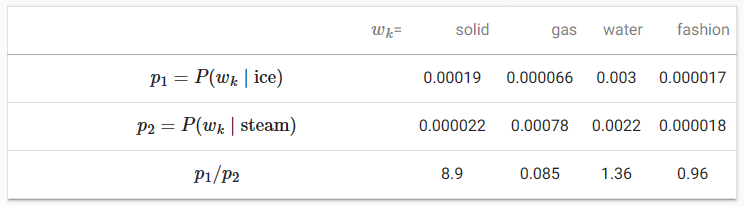
Word-word co-occurrences within context windows may carry rich semantic information. For example, in a large corpus word “solid” is more likely to co-occur with “ice” than “steam”, but word “gas” probably co-occurs with “steam” more frequently than “ice”. Besides, global corpus statistics of such co-occurrences can be precomputed: this can lead to more efficient training. To leverage statistical information in the entire corpus for word embedding, let’s first revisit the skip-gram model in Section 15.1.3, but interpreting it using global corpus statistics such as co-occurrence counts.


15.1. Word Embedding (word2vec) — Dive into Deep Learning 1.0.3 documentation


d2l.ai

컨텍스트 창 내에서 단어-단어 동시 발생 Word-word co-occurrences 은 풍부한 의미 정보를 전달할 수 있습니다. 예를 들어, 대규모 코퍼스에서 "solid"라는 단어는 "steam"보다 "ice"와 함께 나타날 가능성이 더 높지만 "gas"라는 단어는 "ice"보다 "steam"과 더 자주 함께 나타날 가능성이 높습니다. 게다가, 그러한 동시 발생에 대한 글로벌 코퍼스 통계가 미리 계산될 수 있습니다. 이는 보다 효율적인 훈련으로 이어질 수 있습니다. 단어 임베딩을 위해 전체 코퍼스의 통계 정보를 활용하기 위해 먼저 섹션 15.1.3의 스킵 그램 모델을 다시 방문하되 동시 발생 횟수와 같은 전역 코퍼스 통계를 사용하여 해석해 보겠습니다.


15.5.1. Skip-Gram with Global Corpus Statistics


Denoting by qij the conditional probability P(wj∣wi) of word wj given word wi in the skip-gram model, we have this formula where for any index i vectors vi and ui represent word wi as the center word and context word, respectively, and V={0,1,…,|V|−1} is the index set of the vocabulary.


스킵-그램 모델에서 단어 wi가 주어졌을 때 단어 wj의 조건부 확률 P(wj∣wi)를 qij로 표시하면 다음 공식을 얻을 수 있습니다. 여기서 모든 인덱스 i에 대해 벡터 vi와 ui는 단어 wi를 각각 중심 단어와 문맥 단어로 나타냅니다. , 그리고 V={0,1,…,|V|−1}은 어휘의 인덱스 세트입니다.


Consider word wi that may occur multiple times in the corpus. In the entire corpus, all the context words wherever wi is taken as their center word form a multiset Ci of word indices that allows for multiple instances of the same element. For any element, its number of instances is called its multiplicity. To illustrate with an example, suppose that word wi occurs twice in the corpus and indices of the context words that take wi as their center word in the two context windows are k,j,m,k and k,l,k,j. Thus, multiset Ci={j,j,k,k,k,k,l,m}, where multiplicities of elements j,k,l,m are 2, 4, 1, 1, respectively.


말뭉치에서 여러 번 나타날 수 있는 단어 wi를 생각해 보세요. 전체 코퍼스에서 wi가 중심 단어로 사용되는 모든 문맥 단어는 동일한 요소의 여러 인스턴스를 허용하는 단어 인덱스의 다중 집합 Ci를 형성합니다. 모든 요소에 대해 인스턴스 수를 다중성이라고 합니다. 예를 들어 설명하자면, 단어 wi가 말뭉치에 두 번 나타나고 두 문맥 창에서 wi를 중심 단어로 하는 문맥 단어의 인덱스가 k,j,m,k 및 k,l,k,j라고 가정합니다. 따라서 다중 집합 Ci={j,j,k,k,k,k,l,m}이며, 여기서 요소 j,k,l,m의 다중도는 각각 2, 4, 1, 1입니다.


Now let’s denote the multiplicity of element j in multiset Ci as xij. This is the global co-occurrence count of word wj (as the context word) and word wi (as the center word) in the same context window in the entire corpus. Using such global corpus statistics, the loss function of the skip-gram model is equivalent to this fomular,


이제 다중집합 Ci에서 요소 j의 다중도를 xij로 표시해 보겠습니다. 이는 전체 말뭉치에서 동일한 컨텍스트 창에 있는 단어 wj(문맥 단어)와 단어 wi(중앙 단어)의 전역 동시 발생 횟수입니다. 이러한 전역 코퍼스 통계를 사용하면 스킵그램 모델의 손실 함수는 다음 공식과 동일합니다.


We further denote by xi the number of all the context words in the context windows where wi occurs as their center word, which is equivalent to |Ci|. Letting pij be the conditional probability xij/ki for generating context word wj given center word wi, (15.5.2) can be rewritten as


또한 wi가 중심 단어로 나타나는 컨텍스트 창의 모든 컨텍스트 단어 수를 xi로 표시하며 이는 |Ci|와 동일합니다. pij를 중심 단어 wi가 주어졌을 때 문맥 단어 wj를 생성하기 위한 조건부 확률 xij/ki라고 하면 (15.5.2)는 다음 공식으로 다시 작성할 수 있습니다.


In (15.5.3), −∑j∈vpij**log qij calculates the cross-entropy of the conditional distribution pij of global corpus statistics and the conditional distribution qij of model predictions. This loss is also weighted by xi as explained above. Minimizing the loss function in (15.5.3) will allow the predicted conditional distribution to get close to the conditional distribution from the global corpus statistics.


(15.5.3)에서 −∑j∈vpij**log qij는 전역 코퍼스 통계의 조건부 분포 pij와 모델 예측의 조건부 분포 qij의 교차 엔트로피를 계산합니다. 이 손실은 위에서 설명한 대로 xi에 의해 가중치가 부여됩니다. (15.5.3)에서 손실함수를 최소화하면 예측된 조건부 분포가 전역 코퍼스 통계의 조건부 분포에 가까워질 수 있습니다.


Though being commonly used for measuring the distance between probability distributions, the cross-entropy loss function may not be a good choice here. On the one hand, as we mentioned in Section 15.2, the cost of properly normalizing qij results in the sum over the entire vocabulary, which can be computationally expensive. On the other hand, a large number of rare events from a large corpus are often modeled by the cross-entropy loss to be assigned with too much weight.


확률 분포 사이의 거리를 측정하는 데 일반적으로 사용되지만 교차 엔트로피 손실 함수는 여기서는 좋은 선택이 아닐 수 있습니다. 한편으로, 섹션 15.2에서 언급했듯이 qij를 적절하게 정규화하는 비용은 전체 어휘에 대한 합계를 산출하므로 계산 비용이 많이 들 수 있습니다. 반면, 대규모 코퍼스에서 발생하는 다수의 희귀 이벤트는 교차 엔트로피 손실로 모델링되어 너무 많은 가중치가 할당되는 경우가 많습니다.


15.5.2. The GloVe Model


In view of this, the GloVe model makes three changes to the skip-gram model based on squared loss (Pennington et al., 2014):


이를 고려하여 GloVe 모델은 손실 제곱을 기반으로 하는 스킵 그램 모델에 세 가지 변경 사항을 적용합니다(Pennington et al., 2014).


Putting all things together, training GloVe is to minimize the following loss function:


모든 것을 종합하면 GloVe 교육은 다음 손실 함수를 최소화하는 것입니다.


For the weight function, a suggested choice is: ℎ(x)=(x/c)**α (e.g α=0.75) if x<c (e.g., c=100); otherwise ℎ(x)=1. In this case, because ℎ(0)=0, the squared loss term for any xij=0 can be omitted for computational efficiency. For example, when using minibatch stochastic gradient descent for training, at each iteration we randomly sample a minibatch of non-zero xij to calculate gradients and update the model parameters. Note that these non-zero xij are precomputed global corpus statistics; thus, the model is called GloVe for Global Vectors.


가중치 함수의 경우 제안되는 선택은 다음과 같습니다. x<c(예: c=100)인 경우 ℎ(x)=(x/c)**α(예: α=0.75); 그렇지 않으면 ℎ(x)=1입니다. 이 경우 ℎ(0)=0이므로 xij=0에 대한 제곱 손실 항은 계산 효율성을 위해 생략될 수 있습니다. 예를 들어, 훈련을 위해 미니배치 확률적 경사하강법을 사용할 때 각 반복마다 0이 아닌 xij의 미니배치를 무작위로 샘플링하여 경사를 계산하고 모델 매개변수를 업데이트합니다. 0이 아닌 xij는 미리 계산된 글로벌 코퍼스 통계입니다. 따라서 이 모델은 전역 벡터용 GloVe라고 합니다.


It should be emphasized that if word wi appears in the context window of word wj, then vice versa. Therefore, xij=xji. Unlike word2vec that fits the asymmetric conditional probability pij, GloVe fits the symmetric logxij. Therefore, the center word vector and the context word vector of any word are mathematically equivalent in the GloVe model. However in practice, owing to different initialization values, the same word may still get different values in these two vectors after training: GloVe sums them up as the output vector.


wj라는 단어의 컨텍스트 창에 wi라는 단어가 나타나면 그 반대의 경우도 마찬가지라는 점을 강조해야 합니다. 따라서 xij=xji입니다. 비대칭 조건부 확률 pij에 맞는 word2vec와 달리 GloVe는 대칭 logxij에 적합합니다. 따라서 모든 단어의 중심 단어 벡터와 문맥 단어 벡터는 GloVe 모델에서 수학적으로 동일합니다. 그러나 실제로는 초기화 값이 다르기 때문에 동일한 단어가 훈련 후에도 두 벡터에서 서로 다른 값을 얻을 수 있습니다. GloVe는 이를 출력 벡터로 합산합니다.


15.5.3. Interpreting GloVe from the Ratio of Co-occurrence Probabilities

We can also interpret the GloVe model from another perspective. Using the same notation in Section 15.5.1, let pij =def P(wj|wi)  be the conditional probability of generating the context word wj given wi as the center word in the corpus. tab_glove lists several co-occurrence probabilities given words “ice” and “steam” and their ratios based on statistics from a large corpus.


GloVe 모델을 다른 관점에서 해석할 수도 있습니다. 섹션 15.5.1의 동일한 표기법을 사용하여, pij =def P(wj|wi)를 말뭉치의 중심 단어로 wi가 주어진 문맥 단어 wj를 생성하는 조건부 확률로 둡니다. tab_glove는 "ice"와 "steam"이라는 단어가 주어진 여러 동시 발생 확률과 대규모 코퍼스의 통계를 기반으로 한 비율을 나열합니다.


:Word-word co-occurrence probabilities and their ratios from a large corpus (adapted from Table 1 in Pennington et al. (2014))


: 대규모 자료의 단어-단어 동시 발생 확률 및 그 비율(Pennington et al.(2014)의 표 1에서 채택)


Table 15.5.1 label:tab_glove


We can observe the following from tab_glove:


tab_glove에서 다음을 관찰할 수 있습니다.

  • For a word wk that is related to “ice” but unrelated to “steam”, such as wk=solid, we expect a larger ratio of co-occurence probabilities, such as 8.9.
  • wk=solid와 같이 “ice”와 관련이 있지만 “steam”과 관련이 없는 단어 wk의 경우 8.9와 같이 더 큰 동시 발생 확률 비율이 예상됩니다.
  • For a word wk that is related to “steam” but unrelated to “ice”, such as wk=gas, we expect a smaller ratio of co-occurence probabilities, such as 0.085.
  • wk=gas와 같이 "증기"와 관련이 있지만 "얼음"과 관련이 없는 단어 wk의 경우 0.085와 같이 더 작은 동시 발생 확률 비율이 예상됩니다.
  • For a word wk that is related to both “ice” and “steam”, such as wk=water, we expect a ratio of co-occurence probabilities that is close to 1, such as 1.36.
  • wk=물과 같이 "얼음"과 "증기" 모두와 관련된 단어 wk의 경우 1.36과 같이 1에 가까운 동시 발생 확률 비율을 예상합니다.
  • For a word wk that is unrelated to both “ice” and “steam”, such as wk=fashion, we expect a ratio of co-occurence probabilities that is close to 1, such as 0.96.
  • wk=fashion과 같이 "ice"와 "steam" 모두와 관련이 없는 단어 wk의 경우 0.96과 같이 1에 가까운 동시 발생 확률 비율을 기대합니다.

It can be seen that the ratio of co-occurrence probabilities can intuitively express the relationship between words. Thus, we can design a function of three word vectors to fit this ratio. For the ratio of co-occurrence probabilities pij/pik with wi being the center word and wj and wk being the context words, we want to fit this ratio using some function f:


동시발생 확률의 비율을 통해 단어 간의 관계를 직관적으로 표현할 수 있음을 알 수 있다. 따라서 우리는 이 비율에 맞게 세 단어 벡터의 함수를 설계할 수 있습니다. wi가 중심 단어이고 wj와 wk가 문맥 단어인 동시 발생 확률 pij/pik의 비율에 대해 우리는 일부 함수 f를 사용하여 이 비율을 맞추고 싶습니다.


Among many possible designs for f, we only pick a reasonable choice in the following. Since the ratio of co-occurrence probabilities is a scalar, we require that f be a scalar function, such as f(uj,uk,vi)=f((ui−uk)**⊤vi). Switching word indices j and k in (15.5.5), it must hold that f(x)f(−x)=1, so one possibility is f(x)=exp⁡(x), i.e.,


f에 대해 가능한 많은 디자인 중에서 우리는 다음 중에서 합리적인 선택만을 선택합니다. 동시 발생 확률의 비율은 스칼라이므로 f는 f(uj,uk,vi)=f((ui−uk)**⊤vi)와 같은 스칼라 함수여야 합니다. (15.5.5)에서 단어 인덱스 j와 k를 전환하면 f(x)f(−x)=1을 유지해야 하므로 한 가지 가능성은 f(x)=exp⁡(x)입니다. 즉,


Now let’s pick exp⁡(uj**⊤ vi)≈αpij, where α is a constant. Since pij=xij/xi, after taking the logarithm on both sides we get uj**⊤ vi≈log α+log xij − log xi. We may use additional bias terms to fit −log α + log xi, such as the center word bias bi and the context word bias cj:


이제 α가 상수인 exp⁡(uj**⊤ vi)⁡αpij를 선택해 보겠습니다. pij=xij/xi이므로, 양쪽에 로그를 취한 후 uj**⊤ vi≒log α+log xij − log xi를 얻습니다. 중심 단어 바이어스 bi 및 문맥 단어 바이어스 cj와 같이 −log α + log xi를 맞추기 위해 추가 바이어스 항을 사용할 수 있습니다.


Measuring the squared error of (15.5.7) with weights, the GloVe loss function in (15.5.4) is obtained.


가중치를 사용하여 (15.5.7)의 제곱 오차를 측정하면 (15.5.4)의 GloVe 손실 함수가 얻어집니다.


GloVe Model 이란?


The GloVe model, short for Global Vectors for Word Representation, is an unsupervised learning algorithm designed to create word embeddings – numerical representations of words – from large text corpora. These word embeddings capture semantic relationships between words and are used in various natural language processing (NLP) tasks.


GloVe 모델은 Global Vectors for Word Representation의 약자로, 대용량 텍스트 말뭉치에서 단어 임베딩 – 단어의 숫자 표현 – 을 생성하기 위한 비지도 학습 알고리즘입니다. 이러한 단어 임베딩은 단어 간 의미 관계를 포착하며 다양한 자연어 처리 (NLP) 작업에서 사용됩니다.


The key idea behind the GloVe model is to factorize the word co-occurrence matrix, which represents how often words appear together in a given context window. By analyzing these co-occurrence statistics, GloVe learns to embed words in a continuous vector space where similar words are closer to each other, and relationships between words are preserved.


GloVe 모델의 핵심 아이디어는 word co-occurrence matrix을 분해하는 것입니다. 이 행렬은 주어진 문맥 창 내에서 단어가 얼마나 자주 함께 나타나는지를 나타냅니다. 이러한 공기 발생 통계를 분석하여 GloVe는 유사한 단어가 서로 가까이 위치하고 단어 간 관계가 보존되는 연속 벡터 공간에 단어를 임베딩하는 방법을 학습합니다.


Here's a brief overview of how the GloVe model works:


다음은 GloVe 모델의 작동 방식에 대한 간략한 개요입니다:


  1. Construct the Co-occurrence Matrix: Create a co-occurrence matrix that counts how often each word appears in the context of other words within a specified window.

    공기 발생 행렬 생성: 지정된 창 내에서 각 단어가 다른 단어와 함께 나타나는 빈도를 계산하는 공기 발생 행렬을 생성합니다.

  2. Initialize Word Vectors: Initialize word vectors randomly for each word.

    단어 벡터 초기화: 각 단어에 대해 단어 벡터를 무작위로 초기화합니다.

  3. Define the GloVe Objective Function: Define an objective function that measures the difference between the dot product of word vectors and the logarithm of the co-occurrence probabilities. The aim is to minimize the difference.

    GloVe 목적 함수 정의: 단어 벡터의 내적과 공기 발생 확률의 로그 차이를 측정하는 목적 함수를 정의합니다. 목표는 차이를 최소화하는 것입니다.

  4. Optimize the Objective Function: Use an optimization algorithm (usually stochastic gradient descent) to minimize the objective function. During this optimization, the word vectors are updated to better capture the co-occurrence patterns.

    목적 함수 최적화: 최적화 알고리즘 (일반적으로 확률적 경사 하강법)을 사용하여 목적 함수를 최소화합니다. 이 최적화 과정에서 단어 벡터는 공기 발생 패턴을 더 잘 포착하기 위해 업데이트됩니다.

  5. Extract Word Embeddings: Once training is complete, the learned word vectors serve as the word embeddings that capture semantic information about words.

    단어 임베딩 추출: 훈련이 완료되면 학습된 단어 벡터는 의미 정보를 포착하는 단어 임베딩으로 사용됩니다.

GloVe embeddings have gained popularity due to their ability to capture meaningful semantic relationships between words, even without requiring extensive training data. They excel in capturing both syntactic (grammatical) and semantic (meaning-based) relationships, making them useful for a wide range of NLP tasks, such as text classification, sentiment analysis, machine translation, and more.

GloVe 임베딩은 광범위한 의미 관계를 캡처하는 능력으로 인해 풍부한 의미 정보를 기대할 수 없는 환경에서도 의미 있는 의미 관계를 포착하여 인기를 얻었습니다. 구문적 (문법적) 및 의미적 (의미 기반) 관계를 모두 잘 포착하여 텍스트 분류, 감성 분석, 기계 번역 등 다양한 NLP 작업에 유용합니다.

The GloVe model is an important advancement in the field of word embeddings and has contributed significantly to improving the quality of word representations used in various NLP applications.

GloVe 모델은 단어 임베딩 분야에서 중요한 진전으로, 다양한 NLP 응용 프로그램에서 사용되는 단어 표현의 품질을 크게 향상시키는 데 기여한 중요한 역할을 하고 있습니다.


15.5.4. Summary

  • The skip-gram model can be interpreted using global corpus statistics such as word-word co-occurrence counts.

    스킵그램 모델은 단어-단어 동시 발생 횟수와 같은 전역 코퍼스 통계를 사용하여 해석할 수 있습니다.

  • The cross-entropy loss may not be a good choice for measuring the difference of two probability distributions, especially for a large corpus. GloVe uses squared loss to fit precomputed global corpus statistics.

    교차 엔트로피 손실은 특히 대규모 자료의 경우 두 확률 분포의 차이를 측정하는 데 좋은 선택이 아닐 수 있습니다. GloVe는 미리 계산된 글로벌 코퍼스 통계를 맞추기 위해 제곱 손실을 사용합니다.

  • The center word vector and the context word vector are mathematically equivalent for any word in GloVe.

    중심 단어 벡터와 문맥 단어 벡터는 GloVe의 모든 단어에 대해 수학적으로 동일합니다.

  • GloVe can be interpreted from the ratio of word-word co-occurrence probabilities.

    GloVe는 단어-단어 동시 출현 확률의 비율로 해석할 수 있습니다.


15.5.5. Exercises

  1. If words wi and wj co-occur in the same context window, how can we use their distance in the text sequence to redesign the method for calculating the conditional probability pij? Hint: see Section 4.2 of the GloVe paper (Pennington et al., 2014).
  2. For any word, are its center word bias and context word bias mathematically equivalent in GloVe? Why?


반응형


반응형

15.4. Pretraining word2vec — Dive into Deep Learning 1.0.3 documentation (d2l.ai)


15.4. Pretraining word2vec — Dive into Deep Learning 1.0.3 documentation


d2l.ai


15.4. Pretraining word2vec

We go on to implement the skip-gram model defined in Section 15.1. Then we will pretrain word2vec using negative sampling on the PTB dataset. First of all, let’s obtain the data iterator and the vocabulary for this dataset by calling the d2l.load_data_ptb function, which was described in Section 15.3


우리는 계속해서 섹션 15.1에 정의된 스킵 그램 모델을 구현합니다. 그런 다음 PTB 데이터세트에 대해 네거티브 샘플링을 사용하여 word2vec을 사전 학습합니다. 먼저 15.3절에서 설명한 d2l.load_data_ptb 함수를 호출하여 이 데이터셋에 대한 데이터 반복자와 어휘를 구해보겠습니다.


import math
import torch
from torch import nn
from d2l import torch as d2l

batch_size, max_window_size, num_noise_words = 512, 5, 5
data_iter, vocab = d2l.load_data_ptb(batch_size, max_window_size,
                                     num_noise_words)


이 코드는 스킵-그램 모델 학습에 필요한 라이브러리 및 데이터를 불러오고 설정하는 과정을 보여주고 있습니다.

  1. import math, import torch, from torch import nn, from d2l import torch as d2l:
    • math 모듈과 torch 라이브러리의 nn 모듈을 임포트합니다. 또한 d2l 패키지에서 torch 모듈을 가져와 별칭을 d2l로 설정합니다.
  2. batch_size, max_window_size, num_noise_words = 512, 5, 5:
    • 미니배치 크기(batch_size), 최대 윈도우 크기(max_window_size), 부정적 샘플링 개수(num_noise_words)를 각각 512, 5, 5로 설정합니다.
  3. data_iter, vocab = d2l.load_data_ptb(batch_size, max_window_size, num_noise_words):
    • 앞서 설정한 파라미터를 이용하여 d2l.load_data_ptb 함수를 호출하여 PTB 데이터셋을 미니배치 형태로 로드합니다. data_iter는 데이터 로더를 나타내며, vocab은 단어 사전을 나타냅니다.

이 코드는 스킵-그램 모델 학습에 필요한 데이터를 불러오고 설정하는 과정을 보여주고 있습니다.


15.4.1. The Skip-Gram Model

We implement the skip-gram model by using embedding layers and batch matrix multiplications. First, let’s review how embedding layers work.


임베딩 레이어와 배치 행렬 곱셈을 사용하여 스킵 그램 모델을 구현합니다. 먼저 임베딩 레이어의 작동 방식을 살펴보겠습니다.


15.4.1.1. Embedding Layer

As described in Section 10.7, an embedding layer maps a token’s index to its feature vector. The weight of this layer is a matrix whose number of rows equals to the dictionary size (input_dim) and number of columns equals to the vector dimension for each token (output_dim). After a word embedding model is trained, this weight is what we need.


섹션 10.7에 설명된 대로 임베딩 레이어는 토큰의 인덱스를 해당 특징 벡터에 매핑합니다. 이 레이어의 가중치는 행 수가 사전 크기(input_dim)와 같고 열 수가 각 토큰의 벡터 차원(output_dim)과 동일한 행렬입니다. 단어 임베딩 모델이 훈련된 후에는 이 가중치가 우리에게 필요한 것입니다.


embed = nn.Embedding(num_embeddings=20, embedding_dim=4)
print(f'Parameter embedding_weight ({embed.weight.shape}, '
      f'dtype={embed.weight.dtype})')

이 코드는 임베딩 층을 생성하고 해당 임베딩 층의 가중치(weight)의 형태와 데이터 타입을 출력하는 과정을 보여주고 있습니다.

  1. embed = nn.Embedding(num_embeddings=20, embedding_dim=4):
    • nn.Embedding 클래스를 이용하여 임베딩 층(embed)을 생성합니다. num_embeddings는 임베딩할 단어의 개수, embedding_dim은 임베딩된 벡터의 차원을 나타냅니다. 이 코드에서는 20개의 단어를 4차원 벡터로 임베딩하는 임베딩 층을 생성합니다.
  2. print(f'Parameter embedding_weight ({embed.weight.shape}, dtype={embed.weight.dtype})'):
    • 생성한 임베딩 층의 가중치(weight)의 형태와 데이터 타입을 출력합니다. embed.weight는 임베딩 층의 가중치를 나타내며, shape를 통해 가중치의 크기, dtype를 통해 데이터 타입을 확인할 수 있습니다. 이 정보는 임베딩 층의 설정과 가중치를 확인하기 위한 용도로 사용됩니다.

이 코드는 임베딩 층을 생성하고 해당 층의 가중치의 형태와 데이터 타입을 출력하는 과정을 보여주고 있습니다.


The input of an embedding layer is the index of a token (word). For any token index i, its vector representation can be obtained from the ith row of the weight matrix in the embedding layer. Since the vector dimension (output_dim) was set to 4, the embedding layer returns vectors with shape (2, 3, 4) for a minibatch of token indices with shape (2, 3).


임베딩 레이어의 입력은 토큰(단어)의 인덱스입니다. 토큰 인덱스 i의 경우 임베딩 레이어에 있는 가중치 행렬의 i번째 행에서 벡터 표현을 얻을 수 있습니다. 벡터 차원(output_dim)이 4로 설정되었으므로 임베딩 레이어는 모양이 (2, 3)인 토큰 인덱스의 미니 배치에 대해 모양이 (2, 3, 4)인 벡터를 반환합니다.


x = torch.tensor([[1, 2, 3], [4, 5, 6]])
embed(x)

이 코드는 생성한 임베딩 층에 입력 데이터를 넣어 임베딩된 결과를 계산하는 과정을 보여주고 있습니다.

  1. x = torch.tensor([[1, 2, 3], [4, 5, 6]]):
    • 입력 데이터인 2개의 시퀀스를 텐서 형태로 정의합니다. 각 시퀀스는 길이가 3인 정수 시퀀스입니다.
  2. embed(x):
    • 앞서 생성한 임베딩 층 embed에 입력 데이터 x를 넣어서 임베딩된 결과를 계산합니다. 입력 시퀀스에 포함된 각 정수는 해당 정수에 대응하는 임베딩 벡터로 변환됩니다.

임베딩 층을 통해 정수 시퀀스를 임베딩된 벡터로 변환하는 과정을 나타내고 있습니다


15.4.1.2. Defining the Forward Propagation

In the forward propagation, the input of the skip-gram model includes the center word indices center of shape (batch size, 1) and the concatenated context and noise word indices contexts_and_negatives of shape (batch size, max_len), where max_len is defined in Section 15.3.5. These two variables are first transformed from the token indices into vectors via the embedding layer, then their batch matrix multiplication (described in Section 11.3.2.2) returns an output of shape (batch size, 1, max_len). Each element in the output is the dot product of a center word vector and a context or noise word vector.


순방향 전파에서 스킵 그램 모델의 입력에는 center word indices center of shape(배치 크기, 1)과 연결된 컨텍스트 및 노이즈 단어 인덱스 contexts_and_negatives shape(배치 크기, max_len)이 포함됩니다. 여기서 max_len은 다음에서 정의됩니다. 섹션 15.3.5. 이 두 변수는 먼저 임베딩 레이어를 통해 토큰 인덱스에서 벡터로 변환된 다음 배치 행렬 곱셈(섹션 11.3.2.2에 설명됨)이 모양(배치 크기, 1, max_len)의 출력을 반환합니다. 출력의 각 요소는 중심 단어 벡터와 문맥 또는 노이즈 단어 벡터의 내적입니다.


def skip_gram(center, contexts_and_negatives, embed_v, embed_u):
    v = embed_v(center)
    u = embed_u(contexts_and_negatives)
    pred = torch.bmm(v, u.permute(0, 2, 1))
    return pred

이 코드는 스킵-그램 모델의 예측값을 계산하는 함수를 정의하고 있습니다.

  1. def skip_gram(center, contexts_and_negatives, embed_v, embed_u)::
    • skip_gram 함수를 정의합니다. 이 함수는 중심 단어, 문맥 및 부정적 단어 조합, 그리고 중심 단어를 임베딩하는 embed_v와 문맥 및 부정적 단어들을 임베딩하는 embed_u를 인자로 받습니다.
  2. v = embed_v(center):
    • 주어진 중심 단어(center)를 임베딩 벡터로 변환합니다. embed_v를 이용하여 중심 단어를 임베딩합니다.
  3. u = embed_u(contexts_and_negatives):
    • 주어진 문맥 및 부정적 단어 조합(contexts_and_negatives)을 임베딩 벡터로 변환합니다. embed_u를 이용하여 문맥 및 부정적 단어들을 임베딩합니다.
  4. pred = torch.bmm(v, u.permute(0, 2, 1)):
    • 중심 단어 임베딩 벡터 v와 문맥 및 부정적 단어 임베딩 벡터 u 간의 행렬 곱을 계산하여 예측값(pred)을 생성합니다. 행렬 곱은 torch.bmm 함수를 이용하며, 중심 단어의 임베딩 벡터와 각 문맥 및 부정적 단어의 임베딩 벡터 간의 유사도를 나타냅니다.
  5. return pred:
    • 계산한 예측값을 반환합니다.

이 코드는 스킵-그램 모델의 예측값을 계산하는 함수를 정의하고 있습니다.


Let’s print the output shape of this skip_gram function for some example inputs.


몇 가지 예시 입력에 대해 이 Skip_gram 함수의 출력 형태를 인쇄해 보겠습니다.

skip_gram(torch.ones((2, 1), dtype=torch.long),
          torch.ones((2, 4), dtype=torch.long), embed, embed).shape

이 코드는 skip_gram 함수를 사용하여 스킵-그램 모델의 예측값을 계산하고, 계산된 예측값의 형태(shape)를 출력하는 과정을 보여주고 있습니다.

  1. skip_gram(torch.ones((2, 1), dtype=torch.long), torch.ones((2, 4), dtype=torch.long), embed, embed):
    • skip_gram 함수를 호출하여 중심 단어와 문맥 단어의 부정적 샘플들을 이용하여 예측값을 계산합니다. 여기서는 임의의 예시로 중심 단어를 1로, 문맥 및 부정적 단어를 모두 1로 설정하여 호출하였습니다. 이 때, embed 함수를 사용하여 단어들을 임베딩 벡터로 변환합니다.
  2. .shape:
    • 계산된 예측값의 형태(shape)를 확인하는 명령입니다.

이 코드는 skip_gram 함수를 호출하여 스킵-그램 모델의 예측값을 계산하고, 계산된 예측값의 형태(shape)를 출력하는 과정을 나타내고 있습니다


15.4.2. Training

Before training the skip-gram model with negative sampling, let’s first define its loss function.


네거티브 샘플링으로 스킵그램 모델을 훈련하기 전에 먼저 손실 함수를 정의해 보겠습니다.


15.4.2.1. Binary Cross-Entropy Loss

According to the definition of the loss function for negative sampling in Section 15.2.1, we will use the binary cross-entropy loss.


15.2.1절의 네거티브 샘플링에 대한 손실 함수 정의에 따라 이진 교차 엔트로피 손실을 사용합니다.


class SigmoidBCELoss(nn.Module):
    # Binary cross-entropy loss with masking
    def __init__(self):
        super().__init__()

    def forward(self, inputs, target, mask=None):
        out = nn.functional.binary_cross_entropy_with_logits(
            inputs, target, weight=mask, reduction="none")
        return out.mean(dim=1)

loss = SigmoidBCELoss()

이 코드는 마스킹을 적용한 이진 크로스 엔트로피 손실 함수를 정의하고 그 함수를 사용하는 과정을 보여주고 있습니다.

  1. class SigmoidBCELoss(nn.Module)::
    • SigmoidBCELoss 클래스를 정의합니다. 이 클래스는 PyTorch의 nn.Module을 상속하여 정의되었습니다.
  2. def __init__(self)::
    • SigmoidBCELoss 클래스의 초기화 메서드입니다. 별다른 초기화 작업은 없습니다.
  3. def forward(self, inputs, target, mask=None)::
    • forward 메서드는 손실의 계산을 수행합니다. inputs는 모델의 출력, target은 목표값을 나타내며, mask는 선택적으로 적용되는 마스크를 의미합니다.
  4. out = nn.functional.binary_cross_entropy_with_logits(inputs, target, weight=mask, reduction="none"):
    • nn.functional.binary_cross_entropy_with_logits 함수를 사용하여 이진 크로스 엔트로피 손실을 계산합니다. inputs는 모델의 출력, target은 목표값을 나타내며, mask는 선택적으로 적용되는 마스크를 의미합니다. reduction="none"으로 설정하여 요소별 손실 값을 계산합니다.
  5. return out.mean(dim=1):
    • 계산한 손실 값을 각 샘플에 대해 평균내어 반환합니다. dim=1은 각 샘플에 대한 평균을 구하는 축을 나타냅니다.
  6. loss = SigmoidBCELoss():
    • 정의한 SigmoidBCELoss 클래스의 인스턴스를 생성하여 loss 변수에 할당합니다.

이 코드는 마스킹을 적용한 이진 크로스 엔트로피 손실 함수를 정의하고 그 함수를 사용하는 과정을 나타내고 있습니다.


Recall our descriptions of the mask variable and the label variable in Section 15.3.5. The following calculates the binary cross-entropy loss for the given variables.


섹션 15.3.5의 마스크 변수와 라벨 변수에 대한 설명을 떠올려보세요. 다음은 주어진 변수에 대한 이진 교차 엔트로피 손실을 계산합니다.


pred = torch.tensor([[1.1, -2.2, 3.3, -4.4]] * 2)
label = torch.tensor([[1.0, 0.0, 0.0, 0.0], [0.0, 1.0, 0.0, 0.0]])
mask = torch.tensor([[1, 1, 1, 1], [1, 1, 0, 0]])
loss(pred, label, mask) * mask.shape[1] / mask.sum(axis=1)

Below shows how the above results are calculated (in a less efficient way) using the sigmoid activation function in the binary cross-entropy loss. We can consider the two outputs as two normalized losses that are averaged over non-masked predictions.


아래에서는 이진 교차 엔트로피 손실에서 시그모이드 활성화 함수를 사용하여 위 결과를 (덜 효율적인 방식으로) 계산하는 방법을 보여줍니다. 두 개의 출력을 마스크되지 않은 예측에 대해 평균을 낸 두 개의 정규화된 손실로 간주할 수 있습니다.


def sigmd(x):
    return -math.log(1 / (1 + math.exp(-x)))

print(f'{(sigmd(1.1) + sigmd(2.2) + sigmd(-3.3) + sigmd(4.4)) / 4:.4f}')
print(f'{(sigmd(-1.1) + sigmd(-2.2)) / 2:.4f}')


이 코드는 시그모이드 함수를 정의하고, 일부 값들에 대해 시그모이드 함수를 적용한 결과를 출력하는 과정을 보여주고 있습니다.

  1. def sigmd(x)::
    • sigmd 함수를 정의합니다. 이 함수는 시그모이드 함수를 구현한 것으로, 주어진 x에 대해 -math.log(1 / (1 + math.exp(-x))) 값을 반환합니다.
  2. print(f'{(sigmd(1.1) + sigmd(2.2) + sigmd(-3.3) + sigmd(4.4)) / 4:.4f}'):
    • 시그모이드 함수를 각각 1.1, 2.2, -3.3, 4.4에 대해 적용한 결과의 평균을 계산하여 소수점 4자리까지 출력합니다.
  3. print(f'{(sigmd(-1.1) + sigmd(-2.2)) / 2:.4f}'):
    • 시그모이드 함수를 각각 -1.1, -2.2에 대해 적용한 결과의 평균을 계산하여 소수점 4자리까지 출력합니다.

이 코드는 시그모이드 함수를 정의하고, 몇 가지 값들에 대해 이 함수를 적용하여 결과를 출력하는 과정을 나타내고 있습니다


Binary Cross-Entropy Loass란?


Binary Cross-Entropy Loss, often abbreviated as BCE Loss, is a commonly used loss function in machine learning and deep learning, particularly for binary classification tasks. It is used to measure the dissimilarity between the predicted probabilities and the true binary labels of a classification problem.


이진 교차 엔트로피 손실(Binary Cross-Entropy Loss), 줄여서 BCE 손실은 주로 이진 분류 작업에서 사용되는 흔히 쓰이는 손실 함수입니다. 이 함수는 예측된 확률과 실제 이진 레이블 간의 불일치를 측정하는 데 사용됩니다.


In a binary classification problem, each instance belongs to one of two classes, typically denoted as the positive class (1) and the negative class (0). The BCE Loss quantifies the difference between the predicted probabilities of belonging to the positive class and the actual binary labels. It's important to note that BCE Loss is specifically designed for binary classification and not suitable for multi-class classification problems.


이진 분류 작업에서 각 인스턴스는 일반적으로 긍정 클래스(1)와 부정 클래스(0) 중 하나에 속합니다. BCE 손실은 긍정 클래스에 속할 확률의 예측된 값과 실제 이진 레이블 간의 차이를 측정합니다. BCE 손실은 이진 분류에 특화된 것으로, 다중 클래스 분류 작업에는 적합하지 않습니다.


Mathematically, the BCE Loss for a single instance can be defined as follows:

수학적으로 하나의 인스턴스에 대한 BCE 손실은 다음과 같이 정의됩니다:


Where:

  • is the Binary Cross-Entropy Loss.
  • 은 이진 교차 엔트로피 손실입니다.
  • is the true binary label (0 or 1) for the instance.
  • 는 해당 인스턴스의 실제 이진 레이블(0 또는 1)입니다.
  • is the predicted probability of the positive class (i.e., the output of the model's sigmoid activation function).
  • 는 긍정 클래스에 속할 확률의 예측된 값(즉, 모델의 시그모이드 활성화 함수의 출력)입니다.

The loss function is logarithmic in nature, and it penalizes the model more when the predicted probability () deviates from the true label (). The loss is symmetric in the sense that it treats errors of predicting the positive class and predicting the negative class equally.


이 손실 함수는 로그 형태를 띄며, 예측된 확률()이 실제 레이블()에서 얼마나 벗어나는지에 따라 모델을 처벌합니다. 이 손실은 긍정 클래스를 예측하거나 부정 클래스를 예측하는 오류를 동등하게 다루기 때문에 대칭적인 손실입니다.


During training, the goal is to minimize the BCE Loss across all instances in the training dataset. This is typically achieved using optimization algorithms like gradient descent or its variants.


훈련 중에 목표는 훈련 데이터 집합의 모든 인스턴스에 대해 BCE 손실을 최소화하는 것입니다. 이는 일반적으로 경사 하강법 또는 그 변형을 사용하여 달성됩니다.


In summary, Binary Cross-Entropy Loss is a widely used loss function for binary classification problems. It quantifies the difference between predicted probabilities and true binary labels, encouraging the model to improve its predictions and classify instances accurately.


요약하면, 이진 교차 엔트로피 손실은 이진 분류 작업에서 널리 사용되는 손실 함수입니다. 이는 예측된 확률과 실제 이진 레이블 간의 차이를 측정하여 모델이 예측을 향상시키고 인스턴스를 정확하게 분류하도록 유도합니다.


15.4.2.2. Initializing Model Parameters

We define two embedding layers for all the words in the vocabulary when they are used as center words and context words, respectively. The word vector dimension embed_size is set to 100.


우리는 어휘의 모든 단어가 각각 중심 단어와 문맥 단어로 사용될 때 두 개의 임베딩 레이어를 정의합니다. 단어 벡터 차원 embed_size는 100으로 설정됩니다.


embed_size = 100
net = nn.Sequential(nn.Embedding(num_embeddings=len(vocab),
                                 embedding_dim=embed_size),
                    nn.Embedding(num_embeddings=len(vocab),
                                 embedding_dim=embed_size))

이 코드는 임베딩 층을 포함하는 신경망 모델을 생성하는 과정을 나타내고 있습니다.

  1. embed_size = 100:
    • 임베딩 벡터의 차원 크기를 100으로 설정합니다.
  2. net = nn.Sequential(...):
    • nn.Sequential을 사용하여 순차적으로 레이어를 쌓는 모델을 정의합니다.
  3. nn.Embedding(num_embeddings=len(vocab), embedding_dim=embed_size):
    • 첫 번째 임베딩 층을 생성합니다. num_embeddings은 단어 사전(vocab)의 크기, embedding_dim은 임베딩 벡터의 차원 크기를 나타냅니다.
  4. nn.Embedding(num_embeddings=len(vocab), embedding_dim=embed_size):
    • 두 번째 임베딩 층을 생성합니다. 이 층도 첫 번째 임베딩 층과 동일한 설정을 가집니다.

위 코드는 두 개의 임베딩 층을 갖는 신경망 모델을 생성하는 과정을 보여줍니다. 이 모델은 단어를 임베딩 벡터로 변환하는 두 개의 임베딩 층을 포함하고 있습니다.


15.4.2.3. Defining the Training Loop

The training loop is defined below. Because of the existence of padding, the calculation of the loss function is slightly different compared to the previous training functions.


훈련 루프는 아래에 정의되어 있습니다. 패딩이 존재하기 때문에 손실 함수 계산은 이전 훈련 함수와 약간 다릅니다.


def train(net, data_iter, lr, num_epochs, device=d2l.try_gpu()):
    def init_weights(module):
        if type(module) == nn.Embedding:
            nn.init.xavier_uniform_(module.weight)
    net.apply(init_weights)
    net = net.to(device)
    optimizer = torch.optim.Adam(net.parameters(), lr=lr)
    animator = d2l.Animator(xlabel='epoch', ylabel='loss',
                            xlim=[1, num_epochs])
    # Sum of normalized losses, no. of normalized losses
    metric = d2l.Accumulator(2)
    for epoch in range(num_epochs):
        timer, num_batches = d2l.Timer(), len(data_iter)
        for i, batch in enumerate(data_iter):
            optimizer.zero_grad()
            center, context_negative, mask, label = [
                data.to(device) for data in batch]

            pred = skip_gram(center, context_negative, net[0], net[1])
            l = (loss(pred.reshape(label.shape).float(), label.float(), mask)
                     / mask.sum(axis=1) * mask.shape[1])
            l.sum().backward()
            optimizer.step()
            metric.add(l.sum(), l.numel())
            if (i + 1) % (num_batches // 5) == 0 or i == num_batches - 1:
                animator.add(epoch + (i + 1) / num_batches,
                             (metric[0] / metric[1],))
    print(f'loss {metric[0] / metric[1]:.3f}, '
          f'{metric[1] / timer.stop():.1f} tokens/sec on {str(device)}')


이 코드는 스킵-그램 모델을 학습하는 함수를 정의하고 있습니다.

  1. def train(net, data_iter, lr, num_epochs, device=d2l.try_gpu())::
    • train 함수를 정의합니다. 이 함수는 스킵-그램 모델을 학습하는데 필요한 여러 설정값들과 데이터를 받습니다.
  2. def init_weights(module)::
    • 초기화 함수 init_weights를 정의합니다. 이 함수는 네트워크 모델의 가중치 초기화를 수행합니다.
  3. net.apply(init_weights):
    • 네트워크 모델의 가중치를 초기화합니다.
  4. net = net.to(device):
    • 네트워크 모델을 지정한 디바이스로 이동합니다.
  5. optimizer = torch.optim.Adam(net.parameters(), lr=lr):
    • Adam 옵티마이저를 생성합니다.
  6. animator = d2l.Animator(xlabel='epoch', ylabel='loss', xlim=[1, num_epochs]):
    • 학습 과정을 애니메이션으로 표시하기 위한 Animator 객체를 생성합니다.
  7. metric = d2l.Accumulator(2):
    • 손실값을 누적하기 위한 Accumulator 객체를 생성합니다.
  8. 중첩된 반복문:
    • 주어진 에폭 수 만큼 반복하면서 학습을 수행합니다. 내부 반복문은 데이터 배치마다 반복하며 학습을 진행합니다.
  9. optimizer.zero_grad():
    • 옵티마이저의 기울기를 초기화합니다.
  10. 데이터 전처리:
    • 배치 내 데이터들을 지정한 디바이스로 이동합니다.
  11. pred = skip_gram(center, context_negative, net[0], net[1]):
    • skip_gram 함수를 사용하여 스킵-그램 모델의 예측값을 계산합니다.
  12. 손실 계산:
    • 계산된 예측값과 실제 레이블을 이용하여 손실을 계산합니다.
  13. 역전파 및 가중치 업데이트:
    • 손실을 이용하여 역전파를 수행하고 가중치를 업데이트합니다.
  14. 매 에폭 종료 후:
    • 애니메이션에 손실값을 추가하여 학습 과정을 시각화합니다.
  15. 학습 완료 후:
    • 학습이 완료된 후에는 최종 손실값과 학습 속도를 출력합니다.

이 코드는 스킵-그램 모델을 학습하는 함수를 정의하고 있습니다.


Now we can train a skip-gram model using negative sampling.


이제 네거티브 샘플링을 사용하여 스킵그램 모델을 훈련할 수 있습니다.


lr, num_epochs = 0.002, 5
train(net, data_iter, lr, num_epochs)

이 코드는 미리 정의된 train 함수를 사용하여 스킵-그램 모델을 학습하는 과정을 나타내고 있습니다.

  1. lr, num_epochs = 0.002, 5:
    • 학습률(lr)을 0.002로, 에폭 수(num_epochs)를 5로 설정합니다.
  2. train(net, data_iter, lr, num_epochs):
    • 정의된 train 함수를 호출하여 스킵-그램 모델을 학습합니다. net은 학습할 모델, data_iter는 학습 데이터를 제공하는 데이터 반복자, lr은 학습률, num_epochs은 학습 에폭 수를 의미합니다.

즉, 이 코드는 미리 정의된 학습 함수 train을 사용하여 주어진 학습 데이터와 설정값으로 스킵-그램 모델을 학습하는 과정을 나타내고 있습니다.

loss 0.410, 223485.0 tokens/sec on cuda:0


15.4.3. Applying Word Embeddings

After training the word2vec model, we can use the cosine similarity of word vectors from the trained model to find words from the dictionary that are most semantically similar to an input word.


word2vec 모델을 훈련한 후 훈련된 모델의 단어 벡터의 코사인 유사성을 사용하여 입력 단어와 의미상 가장 유사한 사전의 단어를 찾을 수 있습니다.


def get_similar_tokens(query_token, k, embed):
    W = embed.weight.data
    x = W[vocab[query_token]]
    # Compute the cosine similarity. Add 1e-9 for numerical stability
    cos = torch.mv(W, x) / torch.sqrt(torch.sum(W * W, dim=1) *
                                      torch.sum(x * x) + 1e-9)
    topk = torch.topk(cos, k=k+1)[1].cpu().numpy().astype('int32')
    for i in topk[1:]:  # Remove the input words
        print(f'cosine sim={float(cos[i]):.3f}: {vocab.to_tokens(i)}')

get_similar_tokens('chip', 3, net[0])

이 코드는 특정 단어에 대해 유사한 단어를 찾는 함수 get_similar_tokens을 정의하고, 이 함수를 사용하여 주어진 단어와 유사한 단어를 출력하는 과정을 나타내고 있습니다.

  1. def get_similar_tokens(query_token, k, embed)::
    • get_similar_tokens 함수를 정의합니다. 이 함수는 주어진 단어와 유사한 단어를 찾아 출력합니다.
  2. W = embed.weight.data:
    • 임베딩 층의 가중치 정보를 가져옵니다.
  3. x = W[vocab[query_token]]:
    • 주어진 단어의 임베딩 벡터 x를 가져옵니다.
  4. cos = torch.mv(W, x) / torch.sqrt(torch.sum(W * W, dim=1) * torch.sum(x * x) + 1e-9):
    • 코사인 유사도를 계산합니다. 임베딩 벡터들 간의 코사인 유사도를 계산하며, 수치적 안정성을 위해 1e-9를 더해줍니다.
  5. topk = torch.topk(cos, k=k+1)[1].cpu().numpy().astype('int32'):
    • 코사인 유사도에서 가장 높은 상위 k+1개의 값을 가져옵니다. topk에는 상위 값의 인덱스가 저장되어 있습니다.
  6. for i in topk[1:]::
    • 주어진 단어를 제외한 상위 유사한 단어들을 순회하면서 출력합니다.
  7. print(f'cosine sim={float(cos[i]):.3f}: {vocab.to_tokens(i)}'):
    • 각 유사한 단어의 코사인 유사도와 해당 단어를 출력합니다.
  8. get_similar_tokens('chip', 3, net[0]):
    • 'chip' 단어와 유사한 상위 3개의 단어를 찾아 출력합니다.

이 코드는 특정 단어와 유사한 단어를 찾아 출력하는 함수를 정의하고, 이 함수를 사용하여 'chip' 단어와 유사한 단어를 출력하는 과정을 보여주고 있습니다.


cosine sim=0.702: microprocessor
cosine sim=0.649: mips
cosine sim=0.643: intel


15.4.4. Summary


  • We can train a skip-gram model with negative sampling using embedding layers and the binary cross-entropy loss.
  • 임베딩 레이어와 이진 교차 엔트로피 손실을 사용하여 네거티브 샘플링으로 스킵 그램 모델을 훈련할 수 있습니다.
  • Applications of word embeddings include finding semantically similar words for a given word based on the cosine similarity of word vectors.
  • 단어 임베딩의 적용에는 단어 벡터의 코사인 유사성을 기반으로 특정 단어에 대해 의미상 유사한 단어를 찾는 것이 포함됩니다.


15.4.5. Exercises

  1. Using the trained model, find semantically similar words for other input words. Can you improve the results by tuning hyperparameters?
  2. When a training corpus is huge, we often sample context words and noise words for the center words in the current minibatch when updating model parameters. In other words, the same center word may have different context words or noise words in different training epochs. What are the benefits of this method? Try to implement this training method.


반응형


반응형

15.3. The Dataset for Pretraining Word Embeddings — Dive into Deep Learning 1.0.3 documentation (d2l.ai)


15.3. The Dataset for Pretraining Word Embeddings — Dive into Deep Learning 1.0.3 documentation


d2l.ai


15.3. The Dataset for Pretraining Word Embeddings

Now that we know the technical details of the word2vec models and approximate training methods, let’s walk through their implementations. Specifically, we will take the skip-gram model in Section 15.1 and negative sampling in Section 15.2 as an example. In this section, we begin with the dataset for pretraining the word embedding model: the original format of the data will be transformed into minibatches that can be iterated over during training.


이제 word2vec 모델의 기술적 세부 사항과 대략적인 훈련 방법을 알았으므로 구현을 살펴보겠습니다. 구체적으로, 섹션 15.1의 스킵 그램 모델과 섹션 15.2의 네거티브 샘플링을 예로 들어보겠습니다. 이 섹션에서는 단어 임베딩 모델을 사전 훈련하기 위한 데이터 세트부터 시작합니다. 데이터의 원래 형식은 훈련 중에 반복할 수 있는 미니 배치로 변환됩니다.


import collections
import math
import os
import random
import torch
from d2l import torch as d2l


이 코드는 PyTorch와 d2l(Dive into Deep Learning) 라이브러리의 일부 함수들을 사용하여 딥 러닝 모델을 구현하기 위한 환경을 설정하는 부분입니다.

  1. import collections:
    • collections 모듈을 가져옵니다. 이 모듈은 파이썬에서 컨테이너 데이터 타입을 보다 쉽게 다룰 수 있도록 도와주는 클래스들을 제공합니다.
  2. import math:
    • math 모듈을 가져옵니다. 이 모듈은 수학적인 연산을 수행하는 함수들을 제공합니다.
  3. import os:
    • os 모듈을 가져옵니다. 이 모듈은 운영 체제와 관련된 기능을 제공하여 파일 경로, 디렉토리 생성 등을 다루는 데 사용됩니다.
  4. import random:
    • random 모듈을 가져옵니다. 이 모듈은 난수 생성 및 관련된 함수를 제공합니다.
  5. import torch:
    • PyTorch 라이브러리를 가져옵니다. PyTorch는 딥 러닝 모델을 구현하고 훈련하는 데에 사용되는 강력한 라이브러리입니다.
  6. from d2l import torch as d2l:
    • d2l 라이브러리에서 PyTorch와 관련된 함수들을 가져와 d2l이라는 이름으로 사용하겠다는 의미입니다. 이 라이브러리는 "Dive into Deep Learning" 책의 코드와 예제를 포함하고 있는 라이브러리로, 딥 러닝 학습을 돕기 위해 만들어진 것입니다.

이 코드는 여러 모듈과 라이브러리를 가져와서 딥 러닝 모델을 구현하고 실행하기 위한 기반을 설정하는 것입니다.


15.3.1. Reading the Dataset


The dataset that we use here is Penn Tree Bank (PTB). This corpus is sampled from Wall Street Journal articles, split into training, validation, and test sets. In the original format, each line of the text file represents a sentence of words that are separated by spaces. Here we treat each word as a token.


여기서 사용하는 데이터세트는 PTB(Penn Tree Bank)입니다. 이 자료는 Wall Street Journal 기사에서 샘플링되었으며 훈련, 검증 및 테스트 세트로 구분됩니다. 원본 형식에서 텍스트 파일의 각 줄은 공백으로 구분된 단어 문장을 나타냅니다. 여기서는 각 단어를 토큰으로 처리합니다.


#@save
d2l.DATA_HUB['ptb'] = (d2l.DATA_URL + 'ptb.zip',
                       '319d85e578af0cdc590547f26231e4e31cdf1e42')

#@save
def read_ptb():
    """Load the PTB dataset into a list of text lines."""
    data_dir = d2l.download_extract('ptb')
    # Read the training set
    with open(os.path.join(data_dir, 'ptb.train.txt')) as f:
        raw_text = f.read()
    return [line.split() for line in raw_text.split('\n')]

sentences = read_ptb()
f'# sentences: {len(sentences)}'

이 코드는 PTB 데이터셋을 로드하고 텍스트로 처리하는 부분을 보여주고 있습니다.

  1. d2l.DATA_HUB['ptb'] = (d2l.DATA_URL + 'ptb.zip', '319d85e578af0cdc590547f26231e4e31cdf1e42'):
    • d2l.DATA_HUB 딕셔너리에 'ptb'라는 키와 해당 데이터셋의 URL과 해시 값을 저장합니다. 이렇게 함으로써 데이터를 다운로드하고 압축을 해제할 때 사용할 수 있습니다.
  2. def read_ptb()::
    • read_ptb 함수를 정의합니다. 이 함수는 PTB 데이터셋을 로드하고 텍스트를 줄 단위로 분리하여 리스트로 반환합니다.
  3. data_dir = d2l.download_extract('ptb'):
    • d2l.download_extract 함수를 사용하여 PTB 데이터셋을 다운로드하고 압축을 해제합니다. 데이터가 저장될 디렉토리 경로를 data_dir 변수에 저장합니다.
  4. with open(os.path.join(data_dir, 'ptb.train.txt')) as f::
    • PTB 데이터셋 내에 있는 'ptb.train.txt' 파일을 엽니다.
  5. raw_text = f.read():
    • 파일을 읽어서 raw_text 변수에 저장합니다.
  6. return [line.split() for line in raw_text.split('\n')]:
    • raw_text를 줄 단위로 분리한 후 각 줄을 공백으로 분리하여 단어 리스트로 만들어 반환합니다.
  7. sentences = read_ptb():
    • read_ptb 함수를 호출하여 PTB 데이터셋의 텍스트를 처리한 결과를 sentences 변수에 저장합니다.
  8. f'# sentences: {len(sentences)}':
    • 처리된 문장의 개수를 출력하는 문자열을 생성합니다. 이를 통해 문장의 수를 확인할 수 있습니다.


After reading the training set, we build a vocabulary for the corpus, where any word that appears less than 10 times is replaced by the “<unk>” token. Note that the original dataset also contains “<unk>” tokens that represent rare (unknown) words.


훈련 세트를 읽은 후 우리는 10번 미만으로 나타나는 모든 단어가 "<unk>" 토큰으로 대체되는 말뭉치에 대한 어휘를 구축합니다. 원본 데이터세트에는 희귀한(알 수 없는) 단어를 나타내는 “<unk>” 토큰도 포함되어 있습니다.


vocab = d2l.Vocab(sentences, min_freq=10)
f'vocab size: {len(vocab)}'

이 코드는 PTB 데이터셋에서 단어 사전을 생성하는 과정을 나타내고 있습니다.

  1. vocab = d2l.Vocab(sentences, min_freq=10):
    • d2l.Vocab 클래스를 사용하여 단어 사전(vocabulary)을 생성합니다. 이 때 sentences는 PTB 데이터셋에서 읽어온 문장들의 리스트이며, min_freq=10은 최소 빈도수가 10 이상인 단어만을 포함하도록 단어 사전을 구성하겠다는 설정입니다. 이렇게 함으로써