
D2L - 15.4. Pretraining word2vec
2023. 8. 29. 12:23 |
15.4. Pretraining word2vec — Dive into Deep Learning 1.0.3 documentation (d2l.ai)
15.4. Pretraining word2vec — Dive into Deep Learning 1.0.3 documentation
d2l.ai
15.4. Pretraining word2vec
We go on to implement the skip-gram model defined in Section 15.1. Then we will pretrain word2vec using negative sampling on the PTB dataset. First of all, let’s obtain the data iterator and the vocabulary for this dataset by calling the d2l.load_data_ptb function, which was described in Section 15.3
우리는 계속해서 섹션 15.1에 정의된 스킵 그램 모델을 구현합니다. 그런 다음 PTB 데이터세트에 대해 네거티브 샘플링을 사용하여 word2vec을 사전 학습합니다. 먼저 15.3절에서 설명한 d2l.load_data_ptb 함수를 호출하여 이 데이터셋에 대한 데이터 반복자와 어휘를 구해보겠습니다.
import math
import torch
from torch import nn
from d2l import torch as d2l

batch_size, max_window_size, num_noise_words = 512, 5, 5
data_iter, vocab = d2l.load_data_ptb(batch_size, max_window_size,
                                     num_noise_words)
이 코드는 스킵-그램 모델 학습에 필요한 라이브러리 및 데이터를 불러오고 설정하는 과정을 보여주고 있습니다.
- import math, import torch, from torch import nn, from d2l import torch as d2l:
- math 모듈과 torch 라이브러리의 nn 모듈을 임포트합니다. 또한 d2l 패키지에서 torch 모듈을 가져와 별칭을 d2l로 설정합니다.
- batch_size, max_window_size, num_noise_words = 512, 5, 5:
- 미니배치 크기(batch_size), 최대 윈도우 크기(max_window_size), 부정적 샘플링 개수(num_noise_words)를 각각 512, 5, 5로 설정합니다.
- data_iter, vocab = d2l.load_data_ptb(batch_size, max_window_size, num_noise_words):
- 앞서 설정한 파라미터를 이용하여 d2l.load_data_ptb 함수를 호출하여 PTB 데이터셋을 미니배치 형태로 로드합니다. data_iter는 데이터 로더를 나타내며, vocab은 단어 사전을 나타냅니다.
이 코드는 스킵-그램 모델 학습에 필요한 데이터를 불러오고 설정하는 과정을 보여주고 있습니다.
15.4.1. The Skip-Gram Model
We implement the skip-gram model by using embedding layers and batch matrix multiplications. First, let’s review how embedding layers work.
임베딩 레이어와 배치 행렬 곱셈을 사용하여 스킵 그램 모델을 구현합니다. 먼저 임베딩 레이어의 작동 방식을 살펴보겠습니다.
15.4.1.1. Embedding Layer
As described in Section 10.7, an embedding layer maps a token’s index to its feature vector. The weight of this layer is a matrix whose number of rows equals to the dictionary size (input_dim) and number of columns equals to the vector dimension for each token (output_dim). After a word embedding model is trained, this weight is what we need.
섹션 10.7에 설명된 대로 임베딩 레이어는 토큰의 인덱스를 해당 특징 벡터에 매핑합니다. 이 레이어의 가중치는 행 수가 사전 크기(input_dim)와 같고 열 수가 각 토큰의 벡터 차원(output_dim)과 동일한 행렬입니다. 단어 임베딩 모델이 훈련된 후에는 이 가중치가 우리에게 필요한 것입니다.
embed = nn.Embedding(num_embeddings=20, embedding_dim=4)
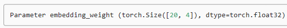
print(f'Parameter embedding_weight ({embed.weight.shape}, '
f'dtype={embed.weight.dtype})')이 코드는 임베딩 층을 생성하고 해당 임베딩 층의 가중치(weight)의 형태와 데이터 타입을 출력하는 과정을 보여주고 있습니다.
- embed = nn.Embedding(num_embeddings=20, embedding_dim=4):
- nn.Embedding 클래스를 이용하여 임베딩 층(embed)을 생성합니다. num_embeddings는 임베딩할 단어의 개수, embedding_dim은 임베딩된 벡터의 차원을 나타냅니다. 이 코드에서는 20개의 단어를 4차원 벡터로 임베딩하는 임베딩 층을 생성합니다.
- print(f'Parameter embedding_weight ({embed.weight.shape}, dtype={embed.weight.dtype})'):
- 생성한 임베딩 층의 가중치(weight)의 형태와 데이터 타입을 출력합니다. embed.weight는 임베딩 층의 가중치를 나타내며, shape를 통해 가중치의 크기, dtype를 통해 데이터 타입을 확인할 수 있습니다. 이 정보는 임베딩 층의 설정과 가중치를 확인하기 위한 용도로 사용됩니다.
이 코드는 임베딩 층을 생성하고 해당 층의 가중치의 형태와 데이터 타입을 출력하는 과정을 보여주고 있습니다.
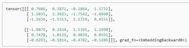
The input of an embedding layer is the index of a token (word). For any token index i, its vector representation can be obtained from the ith row of the weight matrix in the embedding layer. Since the vector dimension (output_dim) was set to 4, the embedding layer returns vectors with shape (2, 3, 4) for a minibatch of token indices with shape (2, 3).
임베딩 레이어의 입력은 토큰(단어)의 인덱스입니다. 토큰 인덱스 i의 경우 임베딩 레이어에 있는 가중치 행렬의 i번째 행에서 벡터 표현을 얻을 수 있습니다. 벡터 차원(output_dim)이 4로 설정되었으므로 임베딩 레이어는 모양이 (2, 3)인 토큰 인덱스의 미니 배치에 대해 모양이 (2, 3, 4)인 벡터를 반환합니다.
x = torch.tensor([[1, 2, 3], [4, 5, 6]])
embed(x)
이 코드는 생성한 임베딩 층에 입력 데이터를 넣어 임베딩된 결과를 계산하는 과정을 보여주고 있습니다.
- x = torch.tensor([[1, 2, 3], [4, 5, 6]]):
- 입력 데이터인 2개의 시퀀스를 텐서 형태로 정의합니다. 각 시퀀스는 길이가 3인 정수 시퀀스입니다.
- embed(x):
- 앞서 생성한 임베딩 층 embed에 입력 데이터 x를 넣어서 임베딩된 결과를 계산합니다. 입력 시퀀스에 포함된 각 정수는 해당 정수에 대응하는 임베딩 벡터로 변환됩니다.
임베딩 층을 통해 정수 시퀀스를 임베딩된 벡터로 변환하는 과정을 나타내고 있습니다
15.4.1.2. Defining the Forward Propagation
In the forward propagation, the input of the skip-gram model includes the center word indices center of shape (batch size, 1) and the concatenated context and noise word indices contexts_and_negatives of shape (batch size, max_len), where max_len is defined in Section 15.3.5. These two variables are first transformed from the token indices into vectors via the embedding layer, then their batch matrix multiplication (described in Section 11.3.2.2) returns an output of shape (batch size, 1, max_len). Each element in the output is the dot product of a center word vector and a context or noise word vector.
순방향 전파에서 스킵 그램 모델의 입력에는 center word indices center of shape(배치 크기, 1)과 연결된 컨텍스트 및 노이즈 단어 인덱스 contexts_and_negatives shape(배치 크기, max_len)이 포함됩니다. 여기서 max_len은 다음에서 정의됩니다. 섹션 15.3.5. 이 두 변수는 먼저 임베딩 레이어를 통해 토큰 인덱스에서 벡터로 변환된 다음 배치 행렬 곱셈(섹션 11.3.2.2에 설명됨)이 모양(배치 크기, 1, max_len)의 출력을 반환합니다. 출력의 각 요소는 중심 단어 벡터와 문맥 또는 노이즈 단어 벡터의 내적입니다.
def skip_gram(center, contexts_and_negatives, embed_v, embed_u):
    v = embed_v(center)
    u = embed_u(contexts_and_negatives)
    pred = torch.bmm(v, u.permute(0, 2, 1))
    return pred
이 코드는 스킵-그램 모델의 예측값을 계산하는 함수를 정의하고 있습니다.
- def skip_gram(center, contexts_and_negatives, embed_v, embed_u)::
- skip_gram 함수를 정의합니다. 이 함수는 중심 단어, 문맥 및 부정적 단어 조합, 그리고 중심 단어를 임베딩하는 embed_v와 문맥 및 부정적 단어들을 임베딩하는 embed_u를 인자로 받습니다.
- v = embed_v(center):
- 주어진 중심 단어(center)를 임베딩 벡터로 변환합니다. embed_v를 이용하여 중심 단어를 임베딩합니다.
- u = embed_u(contexts_and_negatives):
- 주어진 문맥 및 부정적 단어 조합(contexts_and_negatives)을 임베딩 벡터로 변환합니다. embed_u를 이용하여 문맥 및 부정적 단어들을 임베딩합니다.
- pred = torch.bmm(v, u.permute(0, 2, 1)):
- 중심 단어 임베딩 벡터 v와 문맥 및 부정적 단어 임베딩 벡터 u 간의 행렬 곱을 계산하여 예측값(pred)을 생성합니다. 행렬 곱은 torch.bmm 함수를 이용하며, 중심 단어의 임베딩 벡터와 각 문맥 및 부정적 단어의 임베딩 벡터 간의 유사도를 나타냅니다.
- return pred:
- 계산한 예측값을 반환합니다.
이 코드는 스킵-그램 모델의 예측값을 계산하는 함수를 정의하고 있습니다.
Let’s print the output shape of this skip_gram function for some example inputs.
몇 가지 예시 입력에 대해 이 Skip_gram 함수의 출력 형태를 인쇄해 보겠습니다.
skip_gram(torch.ones((2, 1), dtype=torch.long),
          torch.ones((2, 4), dtype=torch.long), embed, embed).shape
이 코드는 skip_gram 함수를 사용하여 스킵-그램 모델의 예측값을 계산하고, 계산된 예측값의 형태(shape)를 출력하는 과정을 보여주고 있습니다.
- skip_gram(torch.ones((2, 1), dtype=torch.long), torch.ones((2, 4), dtype=torch.long), embed, embed):
- skip_gram 함수를 호출하여 중심 단어와 문맥 단어의 부정적 샘플들을 이용하여 예측값을 계산합니다. 여기서는 임의의 예시로 중심 단어를 1로, 문맥 및 부정적 단어를 모두 1로 설정하여 호출하였습니다. 이 때, embed 함수를 사용하여 단어들을 임베딩 벡터로 변환합니다.
- .shape:
- 계산된 예측값의 형태(shape)를 확인하는 명령입니다.
이 코드는 skip_gram 함수를 호출하여 스킵-그램 모델의 예측값을 계산하고, 계산된 예측값의 형태(shape)를 출력하는 과정을 나타내고 있습니다
15.4.2. Training
Before training the skip-gram model with negative sampling, let’s first define its loss function.
네거티브 샘플링으로 스킵그램 모델을 훈련하기 전에 먼저 손실 함수를 정의해 보겠습니다.
15.4.2.1. Binary Cross-Entropy Loss
According to the definition of the loss function for negative sampling in Section 15.2.1, we will use the binary cross-entropy loss.
15.2.1절의 네거티브 샘플링에 대한 손실 함수 정의에 따라 이진 교차 엔트로피 손실을 사용합니다.
class SigmoidBCELoss(nn.Module):
    # Binary cross-entropy loss with masking
    def __init__(self):
        super().__init__()

    def forward(self, inputs, target, mask=None):
        out = nn.functional.binary_cross_entropy_with_logits(
            inputs, target, weight=mask, reduction="none")
        return out.mean(dim=1)

loss = SigmoidBCELoss()
이 코드는 마스킹을 적용한 이진 크로스 엔트로피 손실 함수를 정의하고 그 함수를 사용하는 과정을 보여주고 있습니다.
- class SigmoidBCELoss(nn.Module)::
- SigmoidBCELoss 클래스를 정의합니다. 이 클래스는 PyTorch의 nn.Module을 상속하여 정의되었습니다.
- def __init__(self)::
- SigmoidBCELoss 클래스의 초기화 메서드입니다. 별다른 초기화 작업은 없습니다.
- def forward(self, inputs, target, mask=None)::
- forward 메서드는 손실의 계산을 수행합니다. inputs는 모델의 출력, target은 목표값을 나타내며, mask는 선택적으로 적용되는 마스크를 의미합니다.
- out = nn.functional.binary_cross_entropy_with_logits(inputs, target, weight=mask, reduction="none"):
- nn.functional.binary_cross_entropy_with_logits 함수를 사용하여 이진 크로스 엔트로피 손실을 계산합니다. inputs는 모델의 출력, target은 목표값을 나타내며, mask는 선택적으로 적용되는 마스크를 의미합니다. reduction="none"으로 설정하여 요소별 손실 값을 계산합니다.
- return out.mean(dim=1):
- 계산한 손실 값을 각 샘플에 대해 평균내어 반환합니다. dim=1은 각 샘플에 대한 평균을 구하는 축을 나타냅니다.
- loss = SigmoidBCELoss():
- 정의한 SigmoidBCELoss 클래스의 인스턴스를 생성하여 loss 변수에 할당합니다.
이 코드는 마스킹을 적용한 이진 크로스 엔트로피 손실 함수를 정의하고 그 함수를 사용하는 과정을 나타내고 있습니다.
Recall our descriptions of the mask variable and the label variable in Section 15.3.5. The following calculates the binary cross-entropy loss for the given variables.
섹션 15.3.5의 마스크 변수와 라벨 변수에 대한 설명을 떠올려보세요. 다음은 주어진 변수에 대한 이진 교차 엔트로피 손실을 계산합니다.
pred = torch.tensor([[1.1, -2.2, 3.3, -4.4]] * 2)
label = torch.tensor([[1.0, 0.0, 0.0, 0.0], [0.0, 1.0, 0.0, 0.0]])
mask = torch.tensor([[1, 1, 1, 1], [1, 1, 0, 0]])
loss(pred, label, mask) * mask.shape[1] / mask.sum(axis=1)
Below shows how the above results are calculated (in a less efficient way) using the sigmoid activation function in the binary cross-entropy loss. We can consider the two outputs as two normalized losses that are averaged over non-masked predictions.
아래에서는 이진 교차 엔트로피 손실에서 시그모이드 활성화 함수를 사용하여 위 결과를 (덜 효율적인 방식으로) 계산하는 방법을 보여줍니다. 두 개의 출력을 마스크되지 않은 예측에 대해 평균을 낸 두 개의 정규화된 손실로 간주할 수 있습니다.
def sigmd(x):
    return -math.log(1 / (1 + math.exp(-x)))

print(f'{(sigmd(1.1) + sigmd(2.2) + sigmd(-3.3) + sigmd(4.4)) / 4:.4f}')
print(f'{(sigmd(-1.1) + sigmd(-2.2)) / 2:.4f}')
이 코드는 시그모이드 함수를 정의하고, 일부 값들에 대해 시그모이드 함수를 적용한 결과를 출력하는 과정을 보여주고 있습니다.
- def sigmd(x)::
- sigmd 함수를 정의합니다. 이 함수는 시그모이드 함수를 구현한 것으로, 주어진 x에 대해 -math.log(1 / (1 + math.exp(-x))) 값을 반환합니다.
- print(f'{(sigmd(1.1) + sigmd(2.2) + sigmd(-3.3) + sigmd(4.4)) / 4:.4f}'):
- 시그모이드 함수를 각각 1.1, 2.2, -3.3, 4.4에 대해 적용한 결과의 평균을 계산하여 소수점 4자리까지 출력합니다.
- print(f'{(sigmd(-1.1) + sigmd(-2.2)) / 2:.4f}'):
- 시그모이드 함수를 각각 -1.1, -2.2에 대해 적용한 결과의 평균을 계산하여 소수점 4자리까지 출력합니다.
이 코드는 시그모이드 함수를 정의하고, 몇 가지 값들에 대해 이 함수를 적용하여 결과를 출력하는 과정을 나타내고 있습니다

Binary Cross-Entropy Loass란?
Binary Cross-Entropy Loss, often abbreviated as BCE Loss, is a commonly used loss function in machine learning and deep learning, particularly for binary classification tasks. It is used to measure the dissimilarity between the predicted probabilities and the true binary labels of a classification problem.
이진 교차 엔트로피 손실(Binary Cross-Entropy Loss), 줄여서 BCE 손실은 주로 이진 분류 작업에서 사용되는 흔히 쓰이는 손실 함수입니다. 이 함수는 예측된 확률과 실제 이진 레이블 간의 불일치를 측정하는 데 사용됩니다.
In a binary classification problem, each instance belongs to one of two classes, typically denoted as the positive class (1) and the negative class (0). The BCE Loss quantifies the difference between the predicted probabilities of belonging to the positive class and the actual binary labels. It's important to note that BCE Loss is specifically designed for binary classification and not suitable for multi-class classification problems.
이진 분류 작업에서 각 인스턴스는 일반적으로 긍정 클래스(1)와 부정 클래스(0) 중 하나에 속합니다. BCE 손실은 긍정 클래스에 속할 확률의 예측된 값과 실제 이진 레이블 간의 차이를 측정합니다. BCE 손실은 이진 분류에 특화된 것으로, 다중 클래스 분류 작업에는 적합하지 않습니다.
Mathematically, the BCE Loss for a single instance can be defined as follows:
수학적으로 하나의 인스턴스에 대한 BCE 손실은 다음과 같이 정의됩니다:
Where:
- is the Binary Cross-Entropy Loss.
- 은 이진 교차 엔트로피 손실입니다.
- is the true binary label (0 or 1) for the instance.
- 는 해당 인스턴스의 실제 이진 레이블(0 또는 1)입니다.
- is the predicted probability of the positive class (i.e., the output of the model's sigmoid activation function).
- 는 긍정 클래스에 속할 확률의 예측된 값(즉, 모델의 시그모이드 활성화 함수의 출력)입니다.
The loss function is logarithmic in nature, and it penalizes the model more when the predicted probability () deviates from the true label (). The loss is symmetric in the sense that it treats errors of predicting the positive class and predicting the negative class equally.
이 손실 함수는 로그 형태를 띄며, 예측된 확률()이 실제 레이블()에서 얼마나 벗어나는지에 따라 모델을 처벌합니다. 이 손실은 긍정 클래스를 예측하거나 부정 클래스를 예측하는 오류를 동등하게 다루기 때문에 대칭적인 손실입니다.
During training, the goal is to minimize the BCE Loss across all instances in the training dataset. This is typically achieved using optimization algorithms like gradient descent or its variants.
훈련 중에 목표는 훈련 데이터 집합의 모든 인스턴스에 대해 BCE 손실을 최소화하는 것입니다. 이는 일반적으로 경사 하강법 또는 그 변형을 사용하여 달성됩니다.
In summary, Binary Cross-Entropy Loss is a widely used loss function for binary classification problems. It quantifies the difference between predicted probabilities and true binary labels, encouraging the model to improve its predictions and classify instances accurately.
요약하면, 이진 교차 엔트로피 손실은 이진 분류 작업에서 널리 사용되는 손실 함수입니다. 이는 예측된 확률과 실제 이진 레이블 간의 차이를 측정하여 모델이 예측을 향상시키고 인스턴스를 정확하게 분류하도록 유도합니다.
15.4.2.2. Initializing Model Parameters
We define two embedding layers for all the words in the vocabulary when they are used as center words and context words, respectively. The word vector dimension embed_size is set to 100.
우리는 어휘의 모든 단어가 각각 중심 단어와 문맥 단어로 사용될 때 두 개의 임베딩 레이어를 정의합니다. 단어 벡터 차원 embed_size는 100으로 설정됩니다.
embed_size = 100
net = nn.Sequential(nn.Embedding(num_embeddings=len(vocab),
                                 embedding_dim=embed_size),
                    nn.Embedding(num_embeddings=len(vocab),
                                 embedding_dim=embed_size))
이 코드는 임베딩 층을 포함하는 신경망 모델을 생성하는 과정을 나타내고 있습니다.
- embed_size = 100:
- 임베딩 벡터의 차원 크기를 100으로 설정합니다.
- net = nn.Sequential(...):
- nn.Sequential을 사용하여 순차적으로 레이어를 쌓는 모델을 정의합니다.
- nn.Embedding(num_embeddings=len(vocab), embedding_dim=embed_size):
- 첫 번째 임베딩 층을 생성합니다. num_embeddings은 단어 사전(vocab)의 크기, embedding_dim은 임베딩 벡터의 차원 크기를 나타냅니다.
- nn.Embedding(num_embeddings=len(vocab), embedding_dim=embed_size):
- 두 번째 임베딩 층을 생성합니다. 이 층도 첫 번째 임베딩 층과 동일한 설정을 가집니다.
위 코드는 두 개의 임베딩 층을 갖는 신경망 모델을 생성하는 과정을 보여줍니다. 이 모델은 단어를 임베딩 벡터로 변환하는 두 개의 임베딩 층을 포함하고 있습니다.
15.4.2.3. Defining the Training Loop
The training loop is defined below. Because of the existence of padding, the calculation of the loss function is slightly different compared to the previous training functions.
훈련 루프는 아래에 정의되어 있습니다. 패딩이 존재하기 때문에 손실 함수 계산은 이전 훈련 함수와 약간 다릅니다.
def train(net, data_iter, lr, num_epochs, device=d2l.try_gpu()):
    def init_weights(module):
        if type(module) == nn.Embedding:
            nn.init.xavier_uniform_(module.weight)
    net.apply(init_weights)
    net = net.to(device)
    optimizer = torch.optim.Adam(net.parameters(), lr=lr)
    animator = d2l.Animator(xlabel='epoch', ylabel='loss',
                            xlim=[1, num_epochs])
    # Sum of normalized losses, no. of normalized losses
    metric = d2l.Accumulator(2)
    for epoch in range(num_epochs):
        timer, num_batches = d2l.Timer(), len(data_iter)
        for i, batch in enumerate(data_iter):
            optimizer.zero_grad()
            center, context_negative, mask, label = [
                data.to(device) for data in batch]

            pred = skip_gram(center, context_negative, net[0], net[1])
            l = (loss(pred.reshape(label.shape).float(), label.float(), mask)
                     / mask.sum(axis=1) * mask.shape[1])
            l.sum().backward()
            optimizer.step()
            metric.add(l.sum(), l.numel())
            if (i + 1) % (num_batches // 5) == 0 or i == num_batches - 1:
                animator.add(epoch + (i + 1) / num_batches,
                             (metric[0] / metric[1],))
    print(f'loss {metric[0] / metric[1]:.3f}, '
          f'{metric[1] / timer.stop():.1f} tokens/sec on {str(device)}')
이 코드는 스킵-그램 모델을 학습하는 함수를 정의하고 있습니다.
- def train(net, data_iter, lr, num_epochs, device=d2l.try_gpu())::
- train 함수를 정의합니다. 이 함수는 스킵-그램 모델을 학습하는데 필요한 여러 설정값들과 데이터를 받습니다.
- def init_weights(module)::
- 초기화 함수 init_weights를 정의합니다. 이 함수는 네트워크 모델의 가중치 초기화를 수행합니다.
- net.apply(init_weights):
- 네트워크 모델의 가중치를 초기화합니다.
- net = net.to(device):
- 네트워크 모델을 지정한 디바이스로 이동합니다.
- optimizer = torch.optim.Adam(net.parameters(), lr=lr):
- Adam 옵티마이저를 생성합니다.
- animator = d2l.Animator(xlabel='epoch', ylabel='loss', xlim=[1, num_epochs]):
- 학습 과정을 애니메이션으로 표시하기 위한 Animator 객체를 생성합니다.
- metric = d2l.Accumulator(2):
- 손실값을 누적하기 위한 Accumulator 객체를 생성합니다.
- 중첩된 반복문:
- 주어진 에폭 수 만큼 반복하면서 학습을 수행합니다. 내부 반복문은 데이터 배치마다 반복하며 학습을 진행합니다.
- optimizer.zero_grad():
- 옵티마이저의 기울기를 초기화합니다.
- 데이터 전처리:
- 배치 내 데이터들을 지정한 디바이스로 이동합니다.
- pred = skip_gram(center, context_negative, net[0], net[1]):
- skip_gram 함수를 사용하여 스킵-그램 모델의 예측값을 계산합니다.
- 손실 계산:
- 계산된 예측값과 실제 레이블을 이용하여 손실을 계산합니다.
- 역전파 및 가중치 업데이트:
- 손실을 이용하여 역전파를 수행하고 가중치를 업데이트합니다.
- 매 에폭 종료 후:
- 애니메이션에 손실값을 추가하여 학습 과정을 시각화합니다.
- 학습 완료 후:
- 학습이 완료된 후에는 최종 손실값과 학습 속도를 출력합니다.
이 코드는 스킵-그램 모델을 학습하는 함수를 정의하고 있습니다.
Now we can train a skip-gram model using negative sampling.
이제 네거티브 샘플링을 사용하여 스킵그램 모델을 훈련할 수 있습니다.
lr, num_epochs = 0.002, 5
train(net, data_iter, lr, num_epochs)
이 코드는 미리 정의된 train 함수를 사용하여 스킵-그램 모델을 학습하는 과정을 나타내고 있습니다.
- lr, num_epochs = 0.002, 5:
- 학습률(lr)을 0.002로, 에폭 수(num_epochs)를 5로 설정합니다.
- train(net, data_iter, lr, num_epochs):
- 정의된 train 함수를 호출하여 스킵-그램 모델을 학습합니다. net은 학습할 모델, data_iter는 학습 데이터를 제공하는 데이터 반복자, lr은 학습률, num_epochs은 학습 에폭 수를 의미합니다.
즉, 이 코드는 미리 정의된 학습 함수 train을 사용하여 주어진 학습 데이터와 설정값으로 스킵-그램 모델을 학습하는 과정을 나타내고 있습니다.
loss 0.410, 223485.0 tokens/sec on cuda:0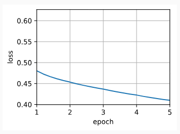
15.4.3. Applying Word Embeddings
After training the word2vec model, we can use the cosine similarity of word vectors from the trained model to find words from the dictionary that are most semantically similar to an input word.
word2vec 모델을 훈련한 후 훈련된 모델의 단어 벡터의 코사인 유사성을 사용하여 입력 단어와 의미상 가장 유사한 사전의 단어를 찾을 수 있습니다.
def get_similar_tokens(query_token, k, embed):
    W = embed.weight.data
    x = W[vocab[query_token]]
    # Compute the cosine similarity. Add 1e-9 for numerical stability
    cos = torch.mv(W, x) / torch.sqrt(torch.sum(W * W, dim=1) *
                                      torch.sum(x * x) + 1e-9)
    topk = torch.topk(cos, k=k+1)[1].cpu().numpy().astype('int32')
    for i in topk[1:]:  # Remove the input words
        print(f'cosine sim={float(cos[i]):.3f}: {vocab.to_tokens(i)}')

get_similar_tokens('chip', 3, net[0])
이 코드는 특정 단어에 대해 유사한 단어를 찾는 함수 get_similar_tokens을 정의하고, 이 함수를 사용하여 주어진 단어와 유사한 단어를 출력하는 과정을 나타내고 있습니다.
- def get_similar_tokens(query_token, k, embed)::
- get_similar_tokens 함수를 정의합니다. 이 함수는 주어진 단어와 유사한 단어를 찾아 출력합니다.
- W = embed.weight.data:
- 임베딩 층의 가중치 정보를 가져옵니다.
- x = W[vocab[query_token]]:
- 주어진 단어의 임베딩 벡터 x를 가져옵니다.
- cos = torch.mv(W, x) / torch.sqrt(torch.sum(W * W, dim=1) * torch.sum(x * x) + 1e-9):
- 코사인 유사도를 계산합니다. 임베딩 벡터들 간의 코사인 유사도를 계산하며, 수치적 안정성을 위해 1e-9를 더해줍니다.
- topk = torch.topk(cos, k=k+1)[1].cpu().numpy().astype('int32'):
- 코사인 유사도에서 가장 높은 상위 k+1개의 값을 가져옵니다. topk에는 상위 값의 인덱스가 저장되어 있습니다.
- for i in topk[1:]::
- 주어진 단어를 제외한 상위 유사한 단어들을 순회하면서 출력합니다.
- print(f'cosine sim={float(cos[i]):.3f}: {vocab.to_tokens(i)}'):
- 각 유사한 단어의 코사인 유사도와 해당 단어를 출력합니다.
- get_similar_tokens('chip', 3, net[0]):
- 'chip' 단어와 유사한 상위 3개의 단어를 찾아 출력합니다.
이 코드는 특정 단어와 유사한 단어를 찾아 출력하는 함수를 정의하고, 이 함수를 사용하여 'chip' 단어와 유사한 단어를 출력하는 과정을 보여주고 있습니다.
cosine sim=0.702: microprocessor
cosine sim=0.649: mips
cosine sim=0.643: intel
15.4.4. Summary
- We can train a skip-gram model with negative sampling using embedding layers and the binary cross-entropy loss.
- 임베딩 레이어와 이진 교차 엔트로피 손실을 사용하여 네거티브 샘플링으로 스킵 그램 모델을 훈련할 수 있습니다.
- Applications of word embeddings include finding semantically similar words for a given word based on the cosine similarity of word vectors.
- 단어 임베딩의 적용에는 단어 벡터의 코사인 유사성을 기반으로 특정 단어에 대해 의미상 유사한 단어를 찾는 것이 포함됩니다.
15.4.5. Exercises
- Using the trained model, find semantically similar words for other input words. Can you improve the results by tuning hyperparameters?
- When a training corpus is huge, we often sample context words and noise words for the center words in the current minibatch when updating model parameters. In other words, the same center word may have different context words or noise words in different training epochs. What are the benefits of this method? Try to implement this training method.
'Dive into Deep Learning > D2L Natural language Processing' 카테고리의 다른 글
| D2L - 15.10. Pretraining BERT (0) | 2023.08.30 |
|---|---|
| D2L - 15.9. The Dataset for Pretraining BERT (0) | 2023.08.30 |
| D2L - 15.8. Bidirectional Encoder Representations from Transformers (BERT) (0) | 2023.08.30 |
| D2L - 15.7. Word Similarity and Analogy (0) | 2023.08.30 |
| D2L - 15.6. Subword Embedding (0) | 2023.08.30 |
| D2L - 15.5. Word Embedding with Global Vectors (GloVe) (0) | 2023.08.29 |
| D2L - 15.3. The Dataset for Pretraining Word Embeddings (0) | 2023.08.29 |
| D2L- 15.2. Approximate Training (0) | 2023.08.28 |
| D2L- 15.1. Word Embedding (word2vec) (0) | 2023.08.25 |
| D2L - 15. Natural Language Processing: Pretraining (0) | 2023.08.24 |