https://d2l.ai/chapter_gaussian-processes/gp-inference.html

18.3. Gaussian Process Inference

In this section, we will show how to perform posterior inference and make predictions using the GP priors we introduced in the last section. We will start with regression, where we can perform inference in closed form. This is a “GPs in a nutshell” section to quickly get up and running with Gaussian processes in practice. We’ll start coding all the basic operations from scratch, and then introduce GPyTorch, which will make working with state-of-the-art Gaussian processes and integration with deep neural networks much more convenient. We will consider these more advanced topics in depth in the next section. In that section, we will also consider settings where approximate inference is required — classification, point processes, or any non-Gaussian likelihoods.

이 섹션에서는 지난 섹션에서 소개한 GP priors 을 사용하여 사후 추론을 수행하고 예측하는 방법을 보여줍니다. 닫힌 형식으로 추론을 수행할 수 있는 회귀부터 시작하겠습니다. 이것은 실제로 가우스 프로세스를 빠르게 시작하고 실행하기 위한 "간단한 GP" 섹션입니다. 모든 기본 작업을 처음부터 코딩하기 시작한 다음 GPyTorch를 소개합니다. 이를 통해 최첨단 가우스 프로세스 작업 및 심층 신경망과의 통합이 훨씬 더 편리해집니다. 다음 섹션에서는 이러한 고급 주제를 심층적으로 고려할 것입니다. 해당 섹션에서는 분류, 포인트 프로세스 또는 비가우시안 가능성 등 대략적인 추론이 필요한 설정도 고려할 것입니다.

Gaussian Process Inference 란?

**가우시안 프로세스 추론(Gaussian Process Inference)**은 기계 학습과 통계 모델링에서 사용되는 강력한 도구 중 하나입니다. 가우시안 프로세스(GP)는 확률적 모델로, 확률 분포의 모든 점을 정의하는 데 사용됩니다. 이것은 특히 회귀 및 분류 문제에 적합하며, 확률 분포의 평균 및 분산을 사용하여 예측을 수행합니다.

여기에서 가우시안 프로세스 추론의 주요 개념을 설명합니다:

1. 프로세스 (Process): 가우시안 프로세스는 "확률적 프로세스"를 모델링하는 것으로 생각할 수 있습니다. 즉, 이는 입력과 출력 간의 관계를 설명하는데 사용되는 확률 모델입니다.
2. 확률 분포: GP는 모든 입력 값에 대한 확률 분포를 정의합니다. 각 입력 값에 대해 출력 값이 가우시안 분포를 따른다고 가정합니다. 따라서 GP는 평균 및 공분산(또는 커널)을 통해 확률 분포를 특성화합니다.
3. 커널 (Kernel): GP의 핵심 부분 중 하나는 커널 함수입니다. 커널 함수는 입력 값 사이의 상관 관계를 정의합니다. 이것은 입력 값 간의 유사성을 측정하고 출력 값의 상관 관계를 결정하는 데 사용됩니다. 일반적으로 RBF(라디얼 베이시스 함수) 커널 또는 신경망 커널 등 다양한 커널 함수를 사용할 수 있습니다.
4. 추론 (Inference): GP는 주어진 입력 값에 대한 출력 값을 추론하는 데 사용됩니다. 기존의 관찰 값을 기반으로 평균 및 분산을 계산하고, 이를 통해 예측값과 예측의 불확실성을 제공합니다. 이러한 예측은 회귀 문제와 분류 문제에서 모두 유용합니다.
5. 하이퍼파라미터 (Hyperparameters): GP는 커널 함수의 하이퍼파라미터를 가집니다. 이러한 하이퍼파라미터는 모델을 학습하는 동안 조정되며, 모델의 적합성을 향상시키기 위해 최적화됩니다.
6. 확률적 예측: GP는 확률적 모델이므로 예측값에 대한 불확실성을 제공합니다. 이것은 예측값이 얼마나 신뢰할 수 있는지를 알려줍니다.

가우시안 프로세스 추론은 주로 회귀 문제를 해결하는 데 사용되며, 데이터에 대한 예측 분포를 생성하여 모델의 불확실성을 고려합니다. 또한 하이퍼파라미터 최적화, 확률적 함수 샘플링 및 데이터 불확실성 추론과 같은 다양한 응용 분야에서 활용됩니다.

18.3.1. Posterior Inference for Regression

An observation model relates the function we want to learn, f(x), to our observations y(x), both indexed by some input x. In classification, x could be the pixels of an image, and y could be the associated class label. In regression, y typically represents a continuous output, such as a land surface temperature, a sea-level, a CO2 concentration, etc.

관측 모델은 우리가 학습하려는 함수 f(x)를 관측값 y(x)에 연결합니다. 둘 다 일부 입력 x에 의해 인덱싱됩니다. 분류에서 x는 이미지의 픽셀이 될 수 있고 y는 관련 클래스 레이블이 될 수 있습니다. 회귀 분석에서 y는 일반적으로 지표면 온도, 해수면, CO2 농도 등과 같은 연속 출력을 나타냅니다.

In regression, we often assume the outputs are given by a latent noise-free function f(x) plus i.i.d. Gaussian noise ϵ(x):

회귀 분석에서 우리는 종종 출력이 잠재 잡음 없는 함수 f(x) + i.i.d로 제공된다고 가정합니다. 가우스 잡음 ϵ(x):

with ϵ(x)∼N(0,σ2). Let y=y(X)=(y(x1),…,y(xn))**⊤ be a vector of our training observations, and f=(f(x1),…,f(xn))**⊤ be a vector of the latent noise-free function values, queried at the training inputs X=x1,…,xn.

ϵ(x)∼N(0,σ2)입니다. y=y(X)=(y(x1),…,y(xn))**⊤를 훈련 관측값의 벡터로 두고 f=(f(x1),…,f(xn))** ⊤ 훈련 입력 X=x1,…,xn에서 쿼리된 잠재 잡음 없는 함수 값의 벡터입니다.

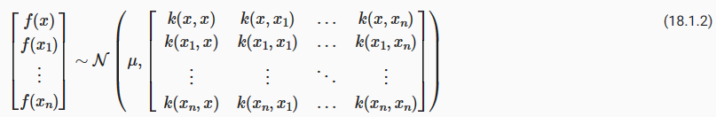
We will assume f(x)∼GP(m,k), which means that any collection of function values f has a joint multivariate Gaussian distribution, with mean vector μi=m(xi) and covariance matrix Kij=k(xi,xj). The RBF kernel k(xi,xj)=a**2 exp⁡(− 1/2ℓ**2||xi−xj||**2) would be a standard choice of covariance function. For notational simplicity, we will assume the mean function m(x)=0; our derivations can easily be generalized later on.

우리는 f(x)∼GP(m,k)를 가정할 것입니다. 이는 f의 모든 함수 값 모음이 평균 벡터 μi=m(xi) 및 공분산 행렬 Kij=k(xi,xj를 갖는 결합 다변량 가우스 분포를 갖는다는 것을 의미합니다. ). RBF 커널 k(xi,xj)=a**2 exp⁡(− 1/2ℓ**2||xi−xj||**2)는 공분산 함수의 표준 선택입니다. 표기를 단순화하기 위해 평균 함수 m(x)=0으로 가정합니다. 우리의 유도는 나중에 쉽게 일반화될 수 있습니다.

Suppose we want to make predictions at a set of inputs

일련의 입력에 대해 예측을 하고 싶다고 가정해 보겠습니다.

Then we want to find x**2 and p(f∗|y,X). In the regression setting, we can conveniently find this distribution by using Gaussian identities, after finding the joint distribution over f∗=f(X∗) and y.

그런 다음 x**2와 p(f*|y,X)를 찾고 싶습니다. 회귀 설정에서 f*=f(X*) 및 y에 대한 결합 분포를 찾은 후 가우스 항등식을 사용하여 이 분포를 편리하게 찾을 수 있습니다.

If we evaluate equation (18.3.1) at the training inputs X, we have y=f+ϵ. By the definition of a Gaussian process (see last section), f∼N(0,K(X,X)) where K(X,X) is an n×n matrix formed by evaluating our covariance function (aka kernel) at all possible pairs of inputs xi,xj∈X. ϵ is simply a vector comprised of iid samples from N(0,σ**2) and thus has distribution N(0,σ**2I). y is therefore a sum of two independent multivariate Gaussian variables, and thus has distribution N(0,K(X,X)+σ**2I). One can also show that cov(f∗,y)=cov(y,f∗)**⊤=K(X∗,X) where K(X∗,X) is an m×n matrix formed by evaluating the kernel at all pairs of test and training inputs.

훈련 입력 X에서 방정식 (18.3.1)을 평가하면 y=f+ϵ가 됩니다. 가우스 프로세스(마지막 섹션 참조)의 정의에 따르면 f∼N(0,K(X,X)) 여기서 K(X,X)는 공분산 함수(일명 커널)를 평가하여 형성된 n×n 행렬입니다. 가능한 모든 입력 쌍 xi,xj∈X. ϵ는 단순히 N(0,σ**2)의 iid 샘플로 구성된 벡터이므로 분포 N(0,σ**2I)를 갖습니다. 따라서 y는 두 개의 독립적인 다변량 가우스 변수의 합이므로 분포 N(0,K(X,X)+σ**2I)를 갖습니다. cov(f*,y)=cov(y,f*)**⊤=K(X*,X) 여기서 K(X*,X)는 커널을 평가하여 형성된 m×n 행렬임을 보여줄 수도 있습니다. 모든 테스트 및 훈련 입력 쌍에서.

We can then use standard Gaussian identities to find the conditional distribution from the joint distribution (see, e.g., Bishop Chapter 2), f∗|y,X,X∗∼N(m∗,S∗), where m∗=K(X∗,X)[K(X,X)+σ**2 I]**−1 y, and S=K(X∗,X∗)−K(X∗,X)[K(X,X)+σ**2 I]**−1 K(X,X∗).

그런 다음 표준 가우스 항등식을 사용하여 결합 분포(예: Bishop 2장 참조) f*|y,X,X*∼N(m*,S*)에서 조건부 분포를 찾을 수 있습니다. 여기서 m*=K (X*,X)[K(X,X)+σ**2 I]**−1 y, S=K(X*,X*)−K(X*,X)[K(X, X)+σ**2 I]**−1 K(X,X**).

Typically, we do not need to make use of the full predictive covariance matrix S, and instead use the diagonal of S for uncertainty about each prediction. Often for this reason we write the predictive distribution for a single test point x∗, rather than a collection of test points.

일반적으로 전체 예측 공분산 행렬 S를 사용할 필요가 없으며 대신 각 예측에 대한 불확실성을 위해 S의 대각선을 사용합니다. 이러한 이유로 우리는 테스트 포인트 모음이 아닌 단일 테스트 포인트 x*에 대한 예측 분포를 작성하는 경우가 많습니다.

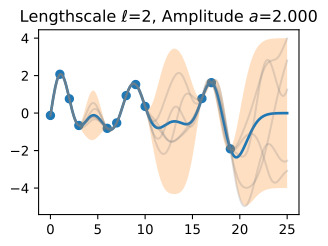
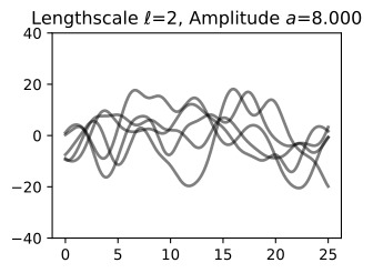
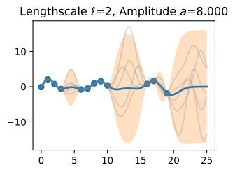
The kernel matrix has parameters θ that we also wish to estimate, such the amplitude 'a' and lengthscale ℓ of the RBF kernel above. For these purposes we use the marginal likelihood, p(y|θ,X), which we already derived in working out the marginal distributions to find the joint distribution over y,f∗. As we will see, the marginal likelihood compartmentalizes into model fit and model complexity terms, and automatically encodes a notion of Occam’s razor for learning hyperparameters. For a full discussion, see MacKay Ch. 28 (MacKay, 2003), and Rasmussen and Williams Ch. 5 (Rasmussen and Williams, 2006).

커널 행렬에는 위의 RBF 커널의 진폭 'a' 및 길이 척도 ℓ와 같이 추정하려는 매개변수 θ가 있습니다. 이러한 목적을 위해 우리는 y,f*에 대한 결합 분포를 찾기 위해 한계 분포를 계산할 때 이미 도출한 한계 우도 p(y|θ,X)를 사용합니다. 앞으로 살펴보겠지만, 한계 우도는 모델 적합성 및 모델 복잡성 용어로 분류되고 하이퍼파라미터 학습을 위한 Occam 면도칼 개념을 자동으로 인코딩합니다. 전체 토론을 보려면 MacKay Ch. 28(MacKay, 2003), Rasmussen 및 Williams Ch. 5 (라스무센과 윌리엄스, 2006).

import math
import os
import gpytorch
import matplotlib.pyplot as plt
import numpy as np
import torch
from scipy import optimize
from scipy.spatial import distance_matrix
from d2l import torch as d2l

d2l.set_figsize()

위의 코드는 여러 Python 라이브러리 및 모듈을 가져오고 환경을 설정하는 부분입니다. 코드의 각 부분에 대한 설명은 다음과 같습니다:

1. import math: Python의 수학 함수와 상수에 액세스하기 위한 라이브러리인 math를 가져옵니다.
2. import os: 운영 체제와 상호 작용하기 위한 라이브러리인 os를 가져옵니다.
3. import gpytorch: Gaussian Process 모델을 구현하고 조작하기 위한 라이브러리인 gpytorch를 가져옵니다. Gaussian Process는 확률 기반 회귀 및 분류 모델링에 사용됩니다.
4. import matplotlib.pyplot as plt: 데이터 시각화를 위한 Matplotlib 라이브러리의 서브 모듈인 pyplot을 가져옵니다.
5. import numpy as np: 다차원 배열 및 수학 함수를 제공하는 NumPy 라이브러리를 가져옵니다.
6. import torch: PyTorch 딥 러닝 라이브러리를 가져옵니다. PyTorch는 신경망 및 텐서 연산을 구현하는 데 사용됩니다.
7. from scipy import optimize: 과학 및 공학 계산을 위한 SciPy 라이브러리의 optimize 모듈을 가져옵니다. 이 모듈은 최적화 문제를 다루는 데 사용됩니다.
8. from scipy.spatial import distance_matrix: SciPy 라이브러리에서 distance_matrix 함수를 가져옵니다. 이 함수는 점들 간의 거리 행렬을 계산하는 데 사용됩니다.
9. from d2l import torch as d2l: "d2l" 모듈에서 "torch" 모듈을 가져옵니다. "d2l" 모듈은 딥 러닝 및 기계 학습 교육을 위한 도구와 함수를 제공합니다.
10. d2l.set_figsize(): D2L(Data Science for Dummies) 라이브러리의 set_figsize 함수를 호출하여 그림의 크기를 설정합니다. 이 함수는 일반적으로 그림의 크기를 조절하기 위해 사용됩니다.

이 코드는 다양한 라이브러리와 모듈을 가져오고, 환경을 설정하여 데이터 분석 및 시각화 작업을 수행할 준비를 하고 있습니다. 이 코드 자체는 데이터를 처리하거나 모델을 구축하지 않으며, 뒤에 나오는 코드 블록에서 작업이 이루어질 것입니다.

Posterior Inference for Regression이란? (GPT 답변)

*Posterior Inference for Regression(회귀를 위한 사후 추론)**는 기계 학습 및 통계에서 주로 사용되는 개념 중 하나입니다. 이것은 회귀 문제에서 예측 모델의 불확실성을 추정하고, 주어진 입력에 대한 출력값의 분포를 모델링하는 프로세스입니다. Posterior Inference는 가우시안 프로세스(GP)와 같은 확률적 모델 또는 베이지안 회귀와 관련이 있습니다. 아래에서 Posterior Inference for Regression의 주요 개념을 설명합니다:

1. 사후 분포(Posterior Distribution): Posterior Inference에서 가장 중요한 개념은 사후 분포입니다. 사후 분포는 모델 파라미터에 대한 확률 분포로, 관찰된 데이터에 대한 정보를 사용하여 업데이트됩니다. 즉, 사후 분포는 관찰된 데이터에 따라 모델 파라미터가 어떻게 업데이트되어야 하는지를 나타냅니다.
2. 베이지안 추론(Bayesian Inference): Posterior Inference는 베이지안 추론의 한 형태입니다. 베이지안 추론은 모델 파라미터의 사후 분포를 계산하는 과정을 포함하며, 이를 통해 모델의 불확실성을 추정합니다.
3. 사후 평균(Posterior Mean): 사후 분포의 평균은 모델 파라미터의 최상의 추정치를 제공합니다. 이것은 예측 모델의 예측값에 대한 추정치로 사용됩니다.
4. 사후 분산(Posterior Variance): 사후 분포의 분산은 모델 파라미터에 대한 불확실성을 나타냅니다. 높은 사후 분산은 모델 파라미터의 불확실성이 크다는 것을 의미하며, 예측의 불확실성에 영향을 미칩니다.
5. 사후 예측(Posterior Prediction): 사후 분포를 사용하여 주어진 입력에 대한 출력값의 분포를 예측합니다. 이것은 예측 모델의 불확실성을 고려하는 중요한 부분입니다.
6. 하이퍼파라미터 최적화(Hyperparameter Optimization): Posterior Inference를 사용하여 모델의 하이퍼파라미터를 최적화할 수 있습니다. 모델의 하이퍼파라미터를 조정하면 모델의 성능을 향상시킬 수 있습니다.

회귀 문제에서 Posterior Inference는 주로 Bayesian 회귀 모델, 가우시안 프로세스 회귀 및 베이지안 최적화에서 사용됩니다. 이를 통해 모델의 예측 불확실성을 고려하여 더 신뢰할 수 있는 예측을 수행할 수 있습니다.

18.3.2. Equations for Making Predictions and Learning Kernel Hyperparameters in GP Regression

We list here the equations you will use for learning hyperparameters and making predictions in Gaussian process regression. Again, we assume a vector of regression targets y, indexed by inputs X={x1,…,xn}, and we wish to make a prediction at a test input x∗. We assume i.i.d. additive zero-mean Gaussian noise with variance σ**2. We use a Gaussian process prior f(x)∼GP(m,k) for the latent noise-free function, with mean function m and kernel function k. The kernel itself has parameters θ that we want to learn. For example, if we use an RBF kernel, k(xi,xj)=a**2 exp⁡(− 1/2ℓ**2||x−x′||**2), we want to learn θ={a**2,ℓ**2}. Let K(X,X) represent an n×n matrix corresponding to evaluating the kernel for all possible pairs of n training inputs. Let K(x∗,X) represent a 1×n vector formed by evaluating k(x∗,xi), i=1,…,n. Let μ be a mean vector formed by evaluating the mean function m(x) at every training points x.

여기에 하이퍼파라미터를 학습하고 가우스 프로세스 회귀에서 예측하는 데 사용할 방정식이 나열되어 있습니다. 다시, 우리는 입력 X={x1,…,xn}에 의해 인덱싱된 회귀 목표 y의 벡터를 가정하고 테스트 입력 x*에서 예측을 만들고 싶습니다. 우리는 i.i.d를 가정합니다. 분산이 σ**2인 가산성 제로 평균 가우스 노이즈. 평균 함수 m과 커널 함수 k를 사용하여 잠재 잡음 없는 함수에 대해 f(x)∼GP(m,k) 이전의 가우스 프로세스를 사용합니다. 커널 자체에는 우리가 배우고 싶은 매개변수 θ가 있습니다. 예를 들어, RBF 커널 k(xi,xj)=a**2 exp⁡(− 1/2ℓ**2||x−x′||**2)를 사용하는 경우 θ=를 배우고 싶습니다. {a**2,ℓ**2}. K(X,X)는 가능한 모든 n 훈련 입력 쌍에 대해 커널을 평가하는 데 해당하는 n×n 행렬을 나타냅니다. K(x*,X)는 k(x*,xi), i=1,…,n을 평가하여 형성된 1×n 벡터를 나타낸다고 가정합니다. μ를 모든 트레이닝 포인트 x에서 평균 함수 m(x)를 평가하여 형성된 평균 벡터로 둡니다.

Typically in working with Gaussian processes, we follow a two-step procedure. 1. Learn kernel hyperparameters θ^ by maximizing the marginal likelihood with respect to these hyperparameters. 2. Use the predictive mean as a point predictor, and 2 times the predictive standard deviation to form a 95% credible set, conditioning on these learned hyperparameters θ^.

일반적으로 가우스 프로세스를 사용하여 작업할 때 우리는 2단계 절차를 따릅니다. 1. 이러한 하이퍼파라미터에 대한 한계 가능성을 최대화하여 커널 하이퍼파라미터 θ^를 학습합니다. 2. 예측 평균을 점 예측 변수로 사용하고 예측 표준 편차의 2배를 사용하여 학습된 하이퍼파라미터 θ^를 조건으로 하여 95% 신뢰할 수 있는 세트를 형성합니다.

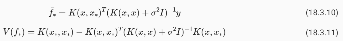
The log marginal likelihood is simply a log Gaussian density, which has the form:

로그 한계 우도는 단순히 로그 가우스 밀도이며 다음과 같은 형식을 갖습니다.

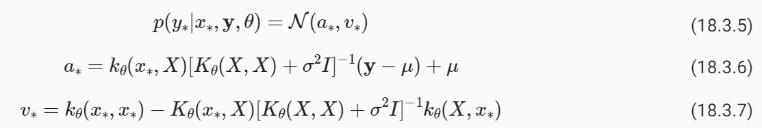
The predictive distribution has the form:

예측 분포의 형식은 다음과 같습니다.

18.3.3. Interpreting Equations for Learning and Predictions

There are some key points to note about the predictive distributions for Gaussian processes:

가우스 프로세스의 예측 분포에 대해 주목해야 할 몇 가지 핵심 사항이 있습니다.

• Despite the flexibility of the model class, it is possible to do exact Bayesian inference for GP regression in closed form. Aside from learning the kernel hyperparameters, there is no training. We can write down exactly what equations we want to use to make predictions. Gaussian processes are relatively exceptional in this respect, and it has greatly contributed to their convenience, versatility, and continued popularity.
  
  모델 클래스의 유연성에도 불구하고 GP 회귀에 대한 정확한 베이지안 추론을 닫힌 형식으로 수행하는 것이 가능합니다. 커널 하이퍼파라미터를 학습하는 것 외에는 교육이 없습니다. 예측을 하기 위해 어떤 방정식을 사용하고 싶은지 정확하게 적을 수 있습니다. 가우스 프로세스는 이 점에서 상대적으로 예외적이며 편의성, 다양성 및 지속적인 인기에 크게 기여했습니다.

• The predictive mean a∗ is a linear combination of the training targets y, weighted by the kernel kθ(x∗,X)[Kθ(x,X)+σ**2 I]**−1. As we will see, the kernel (and its hyperparameters) thus plays a crucial role in the generalization properties of the model.
  
  예측 평균 a*는 커널 kθ(x*,X)[Kθ(x,X)+σ**2 I]**−1에 의해 가중치가 부여된 훈련 목표 y의 선형 조합입니다. 앞으로 살펴보겠지만 커널(및 해당 하이퍼파라미터)은 모델의 일반화 속성에서 중요한 역할을 합니다.

• The predictive mean explicitly depends on the target values y but the predictive variance does not. The predictive uncertainty instead grows as the test input x∗ moves away from the target locations X, as governed by the kernel function. However, uncertainty will implicitly depend on the values of the targets y through the kernel hyperparameters θ, which are learned from the data.
  
  예측 평균은 명시적으로 목표 값 y에 따라 달라지지만 예측 분산은 그렇지 않습니다. 대신 커널 함수에 따라 테스트 입력 x*가 목표 위치 X에서 멀어짐에 따라 예측 불확실성이 커집니다. 그러나 불확실성은 데이터에서 학습된 커널 하이퍼파라미터 θ를 통해 목표 y의 값에 암묵적으로 의존합니다.

• The marginal likelihood compartmentalizes into model fit and model complexity (log determinant) terms. The marginal likelihood tends to select for hyperparameters that provide the simplest fits that are still consistent with the data.
  
  한계 우도는 모델 적합성과 모델 복잡성(로그 결정 요인) 항으로 구분됩니다. 한계 우도는 데이터와 여전히 일치하는 가장 단순한 적합치를 제공하는 초매개변수를 선택하는 경향이 있습니다.

• The key computational bottlenecks come from solving a linear system and computing a log determinant over an n×n symmetric positive definite matrix K(X,X) for n training points. Naively, these operations each incur O(n**3) computations, as well as O(n**2) storage for each entry of the kernel (covariance) matrix, often starting with a Cholesky decomposition. Historically, these bottlenecks have limited GPs to problems with fewer than about 10,000 training points, and have given GPs a reputation for “being slow” that has been inaccurate now for almost a decade. In advanced topics, we will discuss how GPs can be scaled to problems with millions of points.
  
  주요 계산 병목 현상은 선형 시스템을 풀고 n 훈련 포인트에 대한 n×n 대칭 양의 정부호 행렬 K(X,X)에 대한 로그 행렬식을 계산하는 데서 발생합니다. 기본적으로 이러한 작업은 각각 O(n**3) 계산을 발생시키고 커널(공분산) 행렬의 각 항목에 대해 O(n**2) 저장을 발생시키며, 종종 Cholesky 분해로 시작됩니다. 역사적으로 이러한 병목 현상으로 인해 GP는 훈련 포인트가 약 10,000개 미만인 문제로 제한되었으며 GP는 "느리다"는 평판을 얻었으며 현재는 거의 10년 동안 부정확해졌습니다. 고급 주제에서는 GP를 수백만 포인트의 문제로 확장하는 방법에 대해 논의합니다.

• For popular choices of kernel functions, K(X,X) is often close to singular, which can cause numerical issues when performing Cholesky decompositions or other operations intended to solve linear systems. Fortunately, in regression we are often working with Kθ(X,X)+σ**2 I, such that the noise variance σ**2 gets added to the diagonal of K(X,X), significantly improving its conditioning. If the noise variance is small, or we are doing noise free regression, it is common practice to add a small amount of “jitter” to the diagonal, on the order of 10**−6, to improve conditioning.
  
  널리 사용되는 커널 함수 선택의 경우 K(X,X)는 종종 특이값에 가깝습니다. 이는 Cholesky 분해 또는 선형 시스템을 풀기 위한 기타 연산을 수행할 때 수치 문제를 일으킬 수 있습니다. 다행스럽게도 회귀 분석에서는 종종 Kθ(X,X)+σ**2 I로 작업하여 잡음 분산 σ**2가 K(X,X)의 대각선에 추가되어 조건이 크게 향상됩니다. 노이즈 분산이 작거나 노이즈 없는 회귀를 수행하는 경우 컨디셔닝을 개선하기 위해 대각선에 10**−6 정도의 소량의 "지터"를 추가하는 것이 일반적입니다.

18.3.4. Worked Example from Scratch

Let’s create some regression data, and then fit the data with a GP, implementing every step from scratch. We’ll sample data from

회귀 데이터를 생성한 다음 GP로 데이터를 맞추고 모든 단계를 처음부터 구현해 보겠습니다. 다음에서 데이터를 샘플링하겠습니다.

with ϵ∼N(0,σ**2). The noise free function we wish to find is f(x)=sin⁡(x)+1/2 sin⁡(4x). We’ll start by using a noise standard deviation σ=0.25.

ϵ∼N(0,σ**2)입니다. 우리가 찾고자 하는 잡음 없는 함수는 f(x)=sin⁡(x)+1/2 sin⁡(4x)입니다. 잡음 표준편차 σ=0.25를 사용하여 시작하겠습니다.

def data_maker1(x, sig):
    return np.sin(x) + 0.5 * np.sin(4 * x) + np.random.randn(x.shape[0]) * sig

sig = 0.25
train_x, test_x = np.linspace(0, 5, 50), np.linspace(0, 5, 500)
train_y, test_y = data_maker1(train_x, sig=sig), data_maker1(test_x, sig=0.)

d2l.plt.scatter(train_x, train_y)
d2l.plt.plot(test_x, test_y)
d2l.plt.xlabel("x", fontsize=20)
d2l.plt.ylabel("Observations y", fontsize=20)
d2l.plt.show()

위의 코드는 데이터 생성 및 시각화를 수행하는 파이썬 프로그램입니다. 코드의 각 부분에 대한 설명은 다음과 같습니다:

1. def data_maker1(x, sig):: 이 줄은 data_maker1라는 사용자 지정 함수를 정의합니다. 이 함수는 두 개의 입력 매개변수 x와 sig를 받습니다. x는 입력 데이터로 사용되며, sig는 노이즈의 크기를 나타내는 표준 편차입니다.
2. return np.sin(x) + 0.5 * np.sin(4 * x) + np.random.randn(x.shape[0]) * sig: 이 줄은 입력 데이터 x에 대한 관측치를 생성합니다. 관측치는 sin 함수와 4배 주파수가 높은 sin 함수를 합한 값에 노이즈를 추가한 결과입니다. 노이즈는 평균이 0이고 표준 편차가 sig인 정규 분포에서 생성됩니다.
3. sig = 0.25: 이 줄은 데이터 생성에 사용할 노이즈의 크기를 나타내는 sig 변수를 설정합니다. 이 변수는 0.25로 설정되어 있습니다.
4. train_x, test_x = np.linspace(0, 5, 50), np.linspace(0, 5, 500): 이 줄은 학습 데이터와 테스트 데이터의 x 값 범위를 생성합니다. np.linspace 함수를 사용하여 0부터 5까지의 범위를 50개의 등간격으로 분할한 것과 500개의 등간격으로 분할한 것을 각각 train_x와 test_x에 할당합니다.
5. train_y, test_y = data_maker1(train_x, sig=sig), data_maker1(test_x, sig=0.): 이 줄은 data_maker1 함수를 사용하여 학습 데이터와 테스트 데이터에 대한 관측치 train_y와 test_y를 생성합니다. 학습 데이터의 경우 sig 변수 값을 사용하고, 테스트 데이터의 경우 노이즈 없이 생성됩니다.
6. d2l.plt.scatter(train_x, train_y): 이 줄은 학습 데이터를 산점도로 시각화합니다. train_x와 train_y는 x와 y 축에 대한 데이터 포인트를 나타냅니다.
7. d2l.plt.plot(test_x, test_y): 이 줄은 테스트 데이터를 선 그래프로 시각화합니다. test_x와 test_y는 x와 y 축에 대한 데이터 포인트를 나타냅니다.
8. d2l.plt.xlabel("x", fontsize=20) 및 d2l.plt.ylabel("Observations y", fontsize=20): 이 두 줄은 x 축과 y 축에 라벨을 추가하고 글꼴 크기를 설정합니다.
9. d2l.plt.show(): 이 줄은 그래프를 화면에 표시합니다.

이 코드는 sin 함수와 노이즈를 추가하여 가상의 데이터를 생성하고, 학습 데이터와 테스트 데이터를 시각화하여 데이터의 분포를 확인하는 데 사용됩니다.

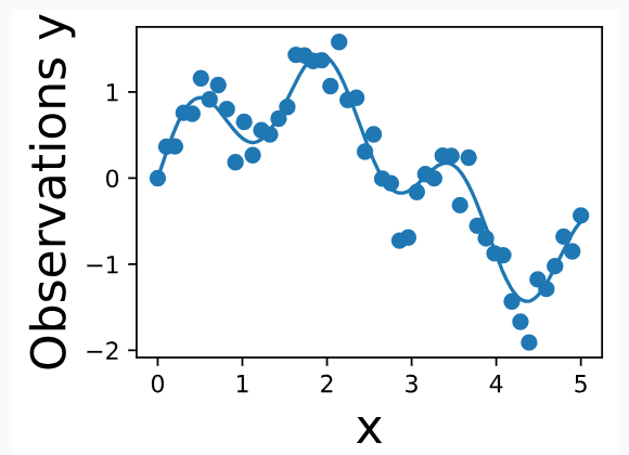
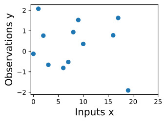
Here we see the noisy observations as circles, and the noise-free function in blue that we wish to find.

여기서는 잡음이 있는 관측값을 원으로 표시하고, 잡음이 없는 함수는 파란색으로 표시합니다.

Now, let’s specify a GP prior over the latent noise-free function, f(x)∼GP(m,k). We’ll use a mean function m(x)=0, and an RBF covariance function (kernel)

이제 잠재 잡음 없는 함수 f(x)∼GP(m,k)보다 먼저 GP를 지정해 보겠습니다. 평균 함수 m(x)=0과 RBF 공분산 함수(커널)를 사용하겠습니다.

mean = np.zeros(test_x.shape[0])
cov = d2l.rbfkernel(test_x, test_x, ls=0.2)

위의 코드는 평균과 공분산 행렬을 계산하는 부분입니다. 이 코드는 Gaussian Process 모델에서 확률 분포를 나타내는 데 사용됩니다. 코드의 각 부분에 대한 설명은 다음과 같습니다:

1. mean = np.zeros(test_x.shape[0]): 이 줄은 mean 변수를 생성하고, 이 변수를 테스트 데이터 포인트 수와 같은 길이의 제로 벡터로 초기화합니다. 이 벡터는 Gaussian Process 모델의 평균을 나타냅니다. 여기서 test_x의 shape[0]은 테스트 데이터 포인트의 수를 나타냅니다.
2. cov = d2l.rbfkernel(test_x, test_x, ls=0.2): 이 줄은 d2l.rbfkernel 함수를 사용하여 테스트 데이터 포인트 간의 공분산 행렬(cov)을 계산합니다. RBF (Radial Basis Function) 커널을 사용하여 계산하며, ls 매개변수는 커널의 길이 스케일을 나타냅니다. 이 커널은 Gaussian Process 모델에서 관측치 간의 상관 관계를 나타냅니다.

결과적으로, mean 변수는 테스트 데이터 포인트에 대한 평균을 나타내고, cov 변수는 테스트 데이터 포인트 간의 공분산을 나타냅니다. 이러한 정보는 Gaussian Process 모델을 구축하고 예측을 수행하는 데 사용됩니다.

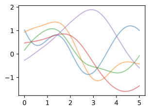
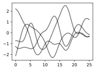
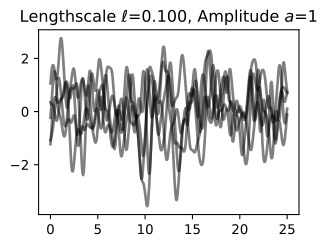
We have started with a length-scale of 0.2. Before we fit the data, it is important to consider whether we have specified a reasonable prior. Let’s visualize some sample functions from this prior, as well as the 95% credible set (we believe there’s a 95% chance that the true function is within this region).

우리는 길이 척도 0.2로 시작했습니다. 데이터를 피팅하기 전에 합리적인 사전 설정을 지정했는지 고려하는 것이 중요합니다. 이전의 일부 샘플 함수와 95% 신뢰할 수 있는 집합을 시각화해 보겠습니다(우리는 실제 함수가 이 영역 내에 있을 확률이 95%라고 믿습니다).

prior_samples = np.random.multivariate_normal(mean=mean, cov=cov, size=5)
d2l.plt.plot(test_x, prior_samples.T, color='black', alpha=0.5)
d2l.plt.plot(test_x, mean, linewidth=2.)
d2l.plt.fill_between(test_x, mean - 2 * np.diag(cov), mean + 2 * np.diag(cov),
                 alpha=0.25)
d2l.plt.show()

위의 코드는 Gaussian Process의 사전 분포를 시각화하기 위한 파이썬 코드입니다. 코드의 각 부분에 대한 설명은 다음과 같습니다:

1. prior_samples = np.random.multivariate_normal(mean=mean, cov=cov, size=5): 이 줄은 np.random.multivariate_normal 함수를 사용하여 Gaussian Process의 사전 분포에서 무작위로 샘플을 생성합니다. 이 샘플은 mean 벡터와 cov 공분산 행렬을 기반으로 생성되며, size=5로 설정하여 5개의 샘플을 생성합니다.
2. d2l.plt.plot(test_x, prior_samples.T, color='black', alpha=0.5): 이 줄은 이전에 생성한 사전 샘플을 시각화합니다. test_x를 x 축으로 하고, 각 샘플을 선 그래프로 표시합니다. color='black'로 설정하여 검은색으로 그림과 alpha=0.5로 설정하여 투명도를 조절합니다.
3. d2l.plt.plot(test_x, mean, linewidth=2.): 이 줄은 Gaussian Process의 평균을 시각화합니다. test_x를 x 축으로 하고 mean을 y 축으로 하는 선 그래프를 그립니다. linewidth=2.로 설정하여 선의 두께를 조절합니다.
4. d2l.plt.fill_between(test_x, mean - 2 * np.diag(cov), mean + 2 * np.diag(cov), alpha=0.25): 이 줄은 Gaussian Process의 신뢰 구간을 시각화합니다. test_x 범위에서 mean - 2 * np.diag(cov)와 mean + 2 * np.diag(cov) 사이를 채우는 영역을 그립니다. 이 영역은 95% 신뢰 구간을 나타내며, alpha=0.25로 설정하여 투명도를 조절합니다.
5. d2l.plt.show(): 이 줄은 그래프를 화면에 표시합니다.

이 코드는 Gaussian Process의 사전 분포를 시각화하여 모델의 예측의 불확실성을 표현합니다. 사전 샘플, 평균 및 신뢰 구간을 통해 모델이 데이터에 대해 어떤 예측을 수행할 수 있는지와 해당 예측의 불확실성을 이해하는 데 도움이 됩니다.

Do these samples look reasonable? Are the high-level properties of the functions aligned with the type of data we are trying to model?

이 샘플이 합리적으로 보입니까? 함수의 상위 수준 속성이 우리가 모델링하려는 데이터 유형과 일치합니까?

Now let’s form the mean and variance of the posterior predictive distribution at any arbitrary test point x∗.

이제 임의의 테스트 지점 x*에서 사후 예측 분포의 평균과 분산을 만들어 보겠습니다.

Before we make predictions, we should learn our kernel hyperparameters θ and noise variance σ**2. Let’s initialize our length-scale at 0.75, as our prior functions looked too quickly varying compared to the data we are fitting. We’ll also guess a noise standard deviation σ of 0.75.

예측을 하기 전에 커널 하이퍼파라미터 θ와 노이즈 분산 σ**2를 배워야 합니다. 이전 함수가 피팅 중인 데이터에 비해 너무 빠르게 변하는 것처럼 보이므로 길이 척도를 0.75로 초기화하겠습니다. 또한 잡음 표준편차 σ를 0.75로 추측하겠습니다.

In order to learn these parameters, we will maximize the marginal likelihood with respect to these parameters.

이러한 매개변수를 학습하기 위해 이러한 매개변수에 대한 한계우도를 최대화하겠습니다.

Perhaps our prior functions were too quickly varying. Let’s guess a length-scale of 0.4. We’ll also guess a noise standard deviation of 0.75. These are simply hyperparameter initializations — we will learn these parameters from the marginal likelihood.

아마도 우리의 이전 기능이 너무 빠르게 변화했을 수도 있습니다. 길이 척도를 0.4로 가정해 보겠습니다. 또한 잡음 표준편차를 0.75로 추측하겠습니다. 이것은 단순히 하이퍼파라미터 초기화입니다. 우리는 이러한 매개변수를 한계 가능성으로부터 학습할 것입니다.

ell_est = 0.4
post_sig_est = 0.5

def neg_MLL(pars):
    K = d2l.rbfkernel(train_x, train_x, ls=pars[0])
    kernel_term = -0.5 * train_y @ \
        np.linalg.inv(K + pars[1] ** 2 * np.eye(train_x.shape[0])) @ train_y
    logdet = -0.5 * np.log(np.linalg.det(K + pars[1] ** 2 * \
                                         np.eye(train_x.shape[0])))
    const = -train_x.shape[0] / 2. * np.log(2 * np.pi)

    return -(kernel_term + logdet + const)


learned_hypers = optimize.minimize(neg_MLL, x0=np.array([ell_est,post_sig_est]),
                                   bounds=((0.01, 10.), (0.01, 10.)))
ell = learned_hypers.x[0]
post_sig_est = learned_hypers.x[1]

위의 코드는 Gaussian Process 모델의 하이퍼파라미터(길이 스케일과 노이즈 수준)를 최적화하기 위한 파이썬 코드입니다. 코드의 각 부분에 대한 설명은 다음과 같습니다:

1. ell_est = 0.4 및 post_sig_est = 0.5: 이 두 줄은 Gaussian Process 모델의 초기 추정치를 설정합니다. ell_est는 길이 스케일을 나타내고, post_sig_est는 노이즈 수준을 나타냅니다.
2. def neg_MLL(pars):: 이 줄은 Gaussian Process 모델의 로그 마이너스 마지널 우도(Log Marginal Likelihood)를 계산하는 사용자 지정 함수 neg_MLL을 정의합니다. 이 함수는 하이퍼파라미터 pars를 입력으로 받습니다.
3. K = d2l.rbfkernel(train_x, train_x, ls=pars[0]): 이 줄은 pars[0] 값을 사용하여 길이 스케일을 설정하고, RBF 커널을 계산합니다. train_x 간의 커널 행렬 K를 생성합니다.
4. kernel_term = -0.5 * train_y @ np.linalg.inv(K + pars[1] ** 2 * np.eye(train_x.shape[0])) @ train_y: 이 줄은 커널 기반 항을 계산합니다. 이 항은 데이터 포인트의 관측치 train_y를 사용하여 계산되며, 커널 행렬 K와 노이즈의 분산을 고려합니다.
5. logdet = -0.5 * np.log(np.linalg.det(K + pars[1] ** 2 * np.eye(train_x.shape[0]))): 이 줄은 로그 행렬식(log determinant)을 계산합니다. 로그 행렬식은 Gaussian Process 모델의 복잡성을 나타내며, 커널 행렬 K와 노이즈의 분산을 고려합니다.
6. const = -train_x.shape[0] / 2. * np.log(2 * np.pi): 이 줄은 상수항을 계산합니다. 이 항은 데이터 포인트의 수와 관련이 있으며, Gaussian Process 모델의 복잡성을 나타냅니다.
7. return -(kernel_term + logdet + const): 이 줄은 로그 마이너스 마지널 우도(negative log marginal likelihood)를 반환합니다. 이 값은 하이퍼파라미터를 조정하여 최소화하려는 목표 함수로 사용됩니다.
8. learned_hypers = optimize.minimize(neg_MLL, x0=np.array([ell_est,post_sig_est]), bounds=((0.01, 10.), (0.01, 10.))): 이 줄은 목표 함수인 neg_MLL를 최소화하여 하이퍼파라미터를 학습하는 과정을 수행합니다. 초기 추정치로 ell_est와 post_sig_est를 사용하고, 각 하이퍼파라미터의 최적 값을 찾기 위해 optimize.minimize 함수를 사용합니다. bounds 매개변수를 사용하여 각 하이퍼파라미터의 최적화 범위를 지정합니다.
9. ell = learned_hypers.x[0]와 post_sig_est = learned_hypers.x[1]: 이 두 줄은 최적화된 하이퍼파라미터 값을 추출합니다. 최적 길이 스케일은 ell 변수에 저장되고, 최적 노이즈 수준은 post_sig_est 변수에 저장됩니다.

이 코드는 Gaussian Process 모델의 하이퍼파라미터를 최적화하여 모델의 예측을 더 정확하게 조정하고 더 좋은 성능을 얻는 데 사용됩니다. 최적화된 하이퍼파라미터는 모델의 복잡성 및 예측의 정확성을 조절하는 데 중요합니다.

In this instance, we learn a length-scale of 0.299, and a noise standard deviation of 0.24. Note that the learned noise is extremely close to the true noise, which helps indicate that our GP is a very well-specified to this problem.

이 경우 길이 척도는 0.299, 잡음 표준 편차는 0.24를 학습합니다. 학습된 잡음은 실제 잡음과 매우 유사하므로 GP가 이 문제에 대해 매우 잘 지정되어 있음을 나타내는 데 도움이 됩니다.

In general, it is crucial to put careful thought into selecting the kernel and initializing the hyperparameters. While marginal likelihood optimization can be relatively robust to initialization, it is not immune to poor initializations. Try running the above script with a variety of initializations and see what results you find.

일반적으로 커널을 선택하고 하이퍼파라미터를 초기화할 때 신중하게 생각하는 것이 중요합니다. 한계 우도 최적화는 초기화에 상대적으로 강력할 수 있지만 잘못된 초기화에는 영향을 받지 않습니다. 다양한 초기화를 사용하여 위 스크립트를 실행해 보고 어떤 결과가 나오는지 확인하세요.

Now, let’s make predictions with these learned hypers.

이제 이러한 학습된 하이퍼를 사용하여 예측을 해보겠습니다.

K_x_xstar = d2l.rbfkernel(train_x, test_x, ls=ell)
K_x_x = d2l.rbfkernel(train_x, train_x, ls=ell)
K_xstar_xstar = d2l.rbfkernel(test_x, test_x, ls=ell)

post_mean = K_x_xstar.T @ np.linalg.inv((K_x_x + \
                post_sig_est ** 2 * np.eye(train_x.shape[0]))) @ train_y
post_cov = K_xstar_xstar - K_x_xstar.T @ np.linalg.inv((K_x_x + \
                post_sig_est ** 2 * np.eye(train_x.shape[0]))) @ K_x_xstar

lw_bd = post_mean - 2 * np.sqrt(np.diag(post_cov))
up_bd = post_mean + 2 * np.sqrt(np.diag(post_cov))

d2l.plt.scatter(train_x, train_y)
d2l.plt.plot(test_x, test_y, linewidth=2.)
d2l.plt.plot(test_x, post_mean, linewidth=2.)
d2l.plt.fill_between(test_x, lw_bd, up_bd, alpha=0.25)
d2l.plt.legend(['Observed Data', 'True Function', 'Predictive Mean', '95% Set on True Func'])
d2l.plt.show()

위의 코드는 Gaussian Process 모델을 사용하여 데이터의 예측을 수행하고 결과를 시각화하는 파이썬 코드입니다. 코드의 각 부분에 대한 설명은 다음과 같습니다:

1. K_x_xstar = d2l.rbfkernel(train_x, test_x, ls=ell): 이 줄은 학습 데이터 train_x와 테스트 데이터 test_x 간의 커널 행렬 K_x_xstar를 계산합니다. 이 커널 행렬은 학습 데이터와 테스트 데이터 간의 상관 관계를 나타냅니다.
2. K_x_x = d2l.rbfkernel(train_x, train_x, ls=ell): 이 줄은 학습 데이터 train_x 간의 커널 행렬 K_x_x를 계산합니다. 이 커널 행렬은 학습 데이터 포인트 간의 상관 관계를 나타냅니다.
3. K_xstar_xstar = d2l.rbfkernel(test_x, test_x, ls=ell): 이 줄은 테스트 데이터 test_x 간의 커널 행렬 K_xstar_xstar를 계산합니다. 이 커널 행렬은 테스트 데이터 포인트 간의 상관 관계를 나타냅니다.
4. post_mean = K_x_xstar.T @ np.linalg.inv((K_x_x + post_sig_est ** 2 * np.eye(train_x.shape[0]))) @ train_y: 이 줄은 예측 평균을 계산합니다. 예측 평균은 테스트 데이터와 학습 데이터 간의 상관 관계를 고려하여 계산되며, train_y는 학습 데이터의 관측치입니다.
5. post_cov = K_xstar_xstar - K_x_xstar.T @ np.linalg.inv((K_x_x + post_sig_est ** 2 * np.eye(train_x.shape[0]))) @ K_x_xstar: 이 줄은 예측 공분산을 계산합니다. 예측 공분산은 테스트 데이터 간의 상관 관계를 고려하여 계산되며, 모델의 불확실성을 나타냅니다.
6. lw_bd = post_mean - 2 * np.sqrt(np.diag(post_cov))와 up_bd = post_mean + 2 * np.sqrt(np.diag(post_cov)): 이 두 줄은 예측 공분산을 기반으로 95% 신뢰 구간을 계산합니다. lw_bd는 신뢰 구간의 하한을 나타내고, up_bd는 신뢰 구간의 상한을 나타냅니다.
7. d2l.plt.scatter(train_x, train_y): 이 줄은 학습 데이터를 산점도로 시각화합니다.
8. d2l.plt.plot(test_x, test_y, linewidth=2.): 이 줄은 테스트 데이터에 대한 실제 함수를 그립니다.
9. d2l.plt.plot(test_x, post_mean, linewidth=2.): 이 줄은 예측 평균을 그립니다.
10. d2l.plt.fill_between(test_x, lw_bd, up_bd, alpha=0.25): 이 줄은 95% 신뢰 구간을 시각화합니다. lw_bd와 up_bd 사이를 채우는 영역을 그립니다.
11. d2l.plt.legend(['Observed Data', 'True Function', 'Predictive Mean', '95% Set on True Func']): 이 줄은 그래프에 범례를 추가합니다.
12. d2l.plt.show(): 이 줄은 그래프를 화면에 표시합니다.

이 코드는 Gaussian Process 모델을 사용하여 데이터의 예측 평균과 신뢰 구간을 계산하고, 학습 데이터, 실제 함수, 예측 평균 및 신뢰 구간을 함께 시각화하여 모델의 예측을 평가합니다.

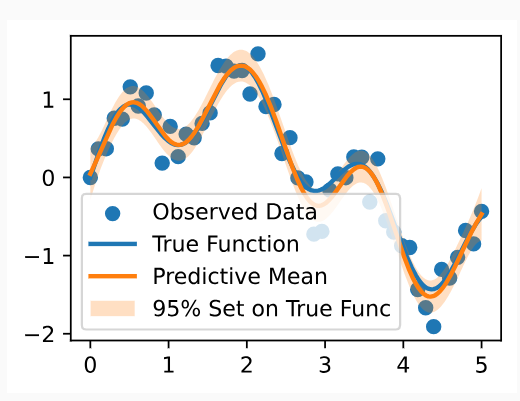
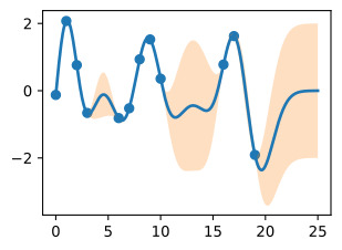
We see the posterior mean in orange almost perfectly matches the true noise free function! Note that the 95% credible set we are showing is for the latent noise free (true) function, and not the data points. We see that this credible set entirely contains the true function, and does not seem overly wide or narrow. We would not want nor expect it to contain the data points. If we wish to have a credible set for the observations, we should compute

주황색의 사후 평균이 실제 노이즈 없는 기능과 거의 완벽하게 일치하는 것을 볼 수 있습니다! 우리가 보여주고 있는 95% 신뢰할 수 있는 세트는 데이터 포인트가 아닌 잠재 잡음 없는(true) 기능에 대한 것입니다. 우리는 이 신뢰할 수 있는 집합이 진정한 기능을 완전히 포함하고 있으며 지나치게 넓거나 좁아 보이지 않는다는 것을 알 수 있습니다. 우리는 데이터 포인트가 포함되는 것을 원하지도 기대하지도 않습니다. 관측값에 대해 신뢰할 수 있는 세트를 갖고 싶다면 다음을 계산해야 합니다.

lw_bd_observed = post_mean - 2 * np.sqrt(np.diag(post_cov) + post_sig_est ** 2)
up_bd_observed = post_mean + 2 * np.sqrt(np.diag(post_cov) + post_sig_est ** 2)

위의 코드는 관찰된 데이터 포인트에 대한 95% 신뢰 구간을 계산하는 부분입니다. 코드의 각 부분에 대한 설명은 다음과 같습니다:

1. lw_bd_observed = post_mean - 2 * np.sqrt(np.diag(post_cov) + post_sig_est ** 2): 이 줄은 하한(낮은 경계) lw_bd_observed를 계산합니다. 이 하한은 예측 평균인 post_mean에서 예측 공분산 행렬 post_cov의 대각 요소에 post_sig_est의 제곱을 더한 값에서 2배의 표준 편차를 뺀 것입니다. 이를 통해 관찰된 데이터 포인트의 예측에 대한 하한을 계산합니다.
2. up_bd_observed = post_mean + 2 * np.sqrt(np.diag(post_cov) + post_sig_est ** 2): 이 줄은 상한(높은 경계) up_bd_observed를 계산합니다. 이 상한은 예측 평균인 post_mean에서 예측 공분산 행렬 post_cov의 대각 요소에 post_sig_est의 제곱을 더한 값에서 2배의 표준 편차를 더한 것입니다. 이를 통해 관찰된 데이터 포인트의 예측에 대한 상한을 계산합니다.

이렇게 계산된 하한과 상한을 사용하면 관찰된 데이터 포인트에 대한 예측의 신뢰 구간을 나타낼 수 있습니다. 이 구간은 모델의 예측의 불확실성을 표현하며, 95%의 신뢰 수준에서 관찰된 데이터 포인트가 포함될 것으로 예상됩니다.

There are two sources of uncertainty, epistemic uncertainty, representing reducible uncertainty, and aleatoric or irreducible uncertainty. The epistemic uncertainty here represents uncertainty about the true values of the noise free function. This uncertainty should grow as we move away from the data points, as away from the data there are a greater variety of function values consistent with our data. As we observe more and more data, our beliefs about the true function become more confident, and the epistemic uncertainty disappears. The aleatoric uncertainty in this instance is the observation noise, since the data are given to us with this noise, and it cannot be reduced.

불확실성에는 두 가지 원인이 있는데, 환원 가능한 불확실성을 나타내는 인식론적 불확실성과 우발적 또는 환원 불가능한 불확실성이 있습니다. 여기서 인식론적 불확실성은 잡음 없는 함수의 실제 값에 대한 불확실성을 나타냅니다. 이러한 불확실성은 데이터 포인트에서 멀어질수록 커집니다. 데이터에서 멀어지면 데이터와 일치하는 더 다양한 함수 값이 있기 때문입니다. 점점 더 많은 데이터를 관찰할수록 실제 함수에 대한 우리의 믿음은 더욱 확신을 갖게 되고 인식론적 불확실성은 사라집니다. 이 경우의 우연적 불확실성은 관찰 잡음입니다. 왜냐하면 데이터가 이 잡음과 함께 우리에게 제공되고 이를 줄일 수 없기 때문입니다.

The epistemic uncertainty in the data is captured by variance of the latent noise free function np.diag(post_cov). The aleatoric uncertainty is captured by the noise variance post_sig_est**2.

데이터의 인식론적 불확실성은 잠재 잡음 없는 함수 np.diag(post_cov)의 분산으로 포착됩니다. 우연적 불확실성은 post_sig_est**2 잡음 분산으로 포착됩니다.

Unfortunately, people are often careless about how they represent uncertainty, with many papers showing error bars that are completely undefined, no clear sense of whether we are visualizing epistemic or aleatoric uncertainty or both, and confusing noise variances with noise standard deviations, standard deviations with standard errors, confidence intervals with credible sets, and so on. Without being precise about what the uncertainty represents, it is essentially meaningless.

불행하게도 사람들은 종종 불확실성을 어떻게 표현하는지에 대해 부주의합니다. 많은 논문에서는 완전히 정의되지 않은 오류 막대가 표시되고, 인식론적 불확실성이나 우연적 불확실성 또는 둘 다를 시각화하고 있는지에 대한 명확한 감각이 없으며, 잡음 분산을 잡음 표준 편차와, 표준 편차를 잡음 표준 편차와 혼동합니다. 표준 오류, 신뢰할 수 있는 세트의 신뢰 구간 등. 불확실성이 무엇을 나타내는지 정확하게 밝히지 않으면 본질적으로 의미가 없습니다.

In the spirit of playing close attention to what our uncertainty represents, it is crucial to note that we are taking two times the square root of our variance estimate for the noise free function. Since our predictive distribution is Gaussian, this quantity enables us to form a 95% credible set, representing our beliefs about the interval which is 95% likely to contain the ground truth function. The noise variance is living on a completely different scale, and is much less interpretable.

불확실성이 무엇을 나타내는지에 세심한 주의를 기울이는 정신으로, 잡음 없는 함수에 대한 분산 추정치의 제곱근의 두 배를 취한다는 점에 유의하는 것이 중요합니다. 예측 분포는 가우스 분포이므로 이 수량을 통해 95% 신뢰할 수 있는 세트를 형성할 수 있으며, 이는 정답 함수를 포함할 가능성이 95%인 구간에 대한 우리의 믿음을 나타냅니다. 노이즈 분산은 완전히 다른 규모로 존재하며 해석하기가 훨씬 어렵습니다.

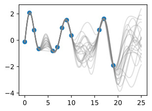
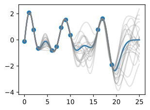
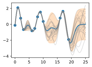
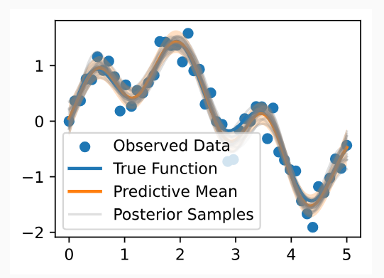
Finally, let’s take a look at 20 posterior samples. These samples tell us what types of functions we believe might fit our data, a posteriori.

마지막으로 20개의 후방 샘플을 살펴보겠습니다. 이 샘플은 어떤 유형의 함수가 데이터에 적합하다고 생각하는지 사후적으로 알려줍니다.

post_samples = np.random.multivariate_normal(post_mean, post_cov, size=20)
d2l.plt.scatter(train_x, train_y)
d2l.plt.plot(test_x, test_y, linewidth=2.)
d2l.plt.plot(test_x, post_mean, linewidth=2.)
d2l.plt.plot(test_x, post_samples.T, color='gray', alpha=0.25)
d2l.plt.fill_between(test_x, lw_bd, up_bd, alpha=0.25)
plt.legend(['Observed Data', 'True Function', 'Predictive Mean', 'Posterior Samples'])
d2l.plt.show()

위의 코드는 Gaussian Process 모델을 사용하여 데이터의 예측을 시각화하는 파이썬 코드입니다. 코드의 각 부분에 대한 설명은 다음과 같습니다:

1. post_samples = np.random.multivariate_normal(post_mean, post_cov, size=20): 이 줄은 post_mean과 post_cov를 기반으로 20개의 사후 샘플을 생성합니다. 이 샘플은 Gaussian Process 모델의 예측 분포에서 무작위로 추출된 것으로, 모델의 불확실성을 반영합니다.
2. d2l.plt.scatter(train_x, train_y): 이 줄은 학습 데이터를 산점도로 시각화합니다.
3. d2l.plt.plot(test_x, test_y, linewidth=2.): 이 줄은 테스트 데이터에 대한 실제 함수를 그립니다.
4. d2l.plt.plot(test_x, post_mean, linewidth=2.): 이 줄은 예측 평균을 그립니다.
5. d2l.plt.plot(test_x, post_samples.T, color='gray', alpha=0.25): 이 줄은 사후 샘플을 그립니다. 사후 샘플은 회색으로 표시되며, 투명도가 조절된 alpha=0.25로 설정되어 있습니다. 이를 통해 모델의 불확실성을 시각화합니다.
6. d2l.plt.fill_between(test_x, lw_bd, up_bd, alpha=0.25): 이 줄은 95% 신뢰 구간을 시각화합니다. lw_bd와 up_bd 사이를 채우는 영역을 그립니다.
7. plt.legend(['Observed Data', 'True Function', 'Predictive Mean', 'Posterior Samples']): 이 줄은 그래프에 범례를 추가합니다. 범례는 'Observed Data' (관찰된 데이터), 'True Function' (실제 함수), 'Predictive Mean' (예측 평균), 'Posterior Samples' (사후 샘플)을 표시합니다.
8. d2l.plt.show(): 이 줄은 그래프를 화면에 표시합니다.

이 코드는 Gaussian Process 모델을 사용하여 데이터의 예측을 시각화하고, 학습 데이터, 실제 함수, 예측 평균, 사후 샘플 및 신뢰 구간을 함께 시각화하여 모델의 예측과 불확실성을 평가합니다. 사후 샘플 및 신뢰 구간은 모델의 예측 분포를 더 자세히 이해하는 데 도움이 됩니다.

In basic regression applications, it is most common to use the posterior predictive mean and standard deviation as a point predictor and metric for uncertainty, respectively. In more advanced applications, such as Bayesian optimization with Monte Carlo acquisition functions, or Gaussian processes for model-based RL, it often necessary to take posterior samples. However, even if not strictly required in the basic applications, these samples give us more intuition about the fit we have for the data, and are often useful to include in visualizations.

기본 회귀 분석에서는 사후 예측 평균과 표준 편차를 각각 점 예측 변수와 불확실성 측정 기준으로 사용하는 것이 가장 일반적입니다. Monte Carlo 획득 기능을 사용한 베이지안 최적화 또는 모델 기반 RL을 위한 가우스 프로세스와 같은 고급 애플리케이션에서는 종종 사후 샘플을 가져와야 하는 경우가 있습니다. 그러나 기본 응용 프로그램에서 엄격하게 요구되지 않더라도 이러한 샘플은 데이터에 대한 적합성에 대해 더 많은 직관을 제공하며 종종 시각화에 포함하는 데 유용합니다.

18.3.5. Making Life Easy with GPyTorch

As we have seen, it is actually pretty easy to implement basic Gaussian process regression entirely from scratch. However, as soon as we want to explore a variety of kernel choices, consider approximate inference (which is needed even for classification), combine GPs with neural networks, or even have a dataset larger than about 10,000 points, then an implementation from scratch becomes unwieldy and cumbersome. Some of the most effective methods for scalable GP inference, such as SKI (also known as KISS-GP), can require hundreds of lines of code implementing advanced numerical linear algebra routines.

우리가 본 것처럼 기본 가우스 프로세스 회귀를 처음부터 완전히 구현하는 것은 실제로 매우 쉽습니다. 그러나 다양한 커널 선택을 탐색하고, 대략적인 추론(분류에도 필요함)을 고려하고, GP를 신경망과 결합하거나, 심지어 약 10,000포인트보다 큰 데이터 세트를 갖고자 하는 경우, 처음부터 다시 구현해야 합니다. 다루기 힘들고 번거롭다. SKI(KISS-GP라고도 함)와 같은 확장 가능한 GP 추론을 위한 가장 효과적인 방법 중 일부에는 고급 수치 선형 대수 루틴을 구현하는 수백 줄의 코드가 필요할 수 있습니다.

In these cases, the GPyTorch library will make our lives a lot easier. We’ll be discussing GPyTorch more in future notebooks on Gaussian process numerics, and advanced methods. The GPyTorch library contains many examples. To get a feel for the package, we will walk through the simple regression example, showing how it can be adapted to reproduce our above results using GPyTorch. This may seem like a lot of code to simply reproduce the basic regression above, and in a sense, it is. But we can immediately use a variety of kernels, scalable inference techniques, and approximate inference, by only changing a few lines of code from below, instead of writing potentially thousands of lines of new code.

이러한 경우 GPyTorch 라이브러리는 우리 삶을 훨씬 쉽게 만들어 줄 것입니다. 우리는 가우스 프로세스 수치 및 고급 방법에 대한 향후 노트북에서 GPyTorch에 대해 더 많이 논의할 것입니다. GPyTorch 라이브러리에는 많은 예제가 포함되어 있습니다. 패키지에 대한 느낌을 얻기 위해 간단한 회귀 예제를 살펴보고 GPyTorch를 사용하여 위 결과를 재현하도록 어떻게 적용할 수 있는지 보여드리겠습니다. 이는 위의 기본 회귀를 간단히 재현하기에는 많은 코드처럼 보일 수 있으며 어떤 의미에서는 그렇습니다. 그러나 잠재적으로 수천 줄의 새로운 코드를 작성하는 대신 아래에서 몇 줄의 코드만 변경하면 다양한 커널, 확장 가능한 추론 기술 및 대략적인 추론을 즉시 사용할 수 있습니다.

# First let's convert our data into tensors for use with PyTorch
train_x = torch.tensor(train_x)
train_y = torch.tensor(train_y)
test_y = torch.tensor(test_y)

# We are using exact GP inference with a zero mean and RBF kernel
class ExactGPModel(gpytorch.models.ExactGP):
    def __init__(self, train_x, train_y, likelihood):
        super(ExactGPModel, self).__init__(train_x, train_y, likelihood)
        self.mean_module = gpytorch.means.ZeroMean()
        self.covar_module = gpytorch.kernels.ScaleKernel(
            gpytorch.kernels.RBFKernel())

    def forward(self, x):
        mean_x = self.mean_module(x)
        covar_x = self.covar_module(x)
        return gpytorch.distributions.MultivariateNormal(mean_x, covar_x)

위의 코드는 PyTorch와 GPyTorch를 사용하여 정확한 Gaussian Process(GP) 모델을 정의하는 파트입니다. 코드의 각 부분에 대한 설명은 다음과 같습니다:

1. 데이터를 PyTorch Tensor로 변환하는 부분:
   • train_x = torch.tensor(train_x): 학습 데이터 train_x를 PyTorch Tensor로 변환합니다.
   • train_y = torch.tensor(train_y): 학습 데이터의 관측치 train_y를 PyTorch Tensor로 변환합니다.
   • test_y = torch.tensor(test_y): 테스트 데이터의 관측치 test_y를 PyTorch Tensor로 변환합니다. (주의: 테스트 데이터의 test_x는 변환되지 않았으므로 주의가 필요합니다.)
2. 정확한 GP 모델 정의:
   • class ExactGPModel(gpytorch.models.ExactGP):: ExactGP 클래스를 상속받는 새로운 GP 모델 클래스 ExactGPModel을 정의합니다. 이 클래스는 GPyTorch를 사용하여 정확한 GP 추론을 수행합니다.
   • def __init__(self, train_x, train_y, likelihood):: 모델의 생성자 메서드에서 학습 데이터 train_x, 관측치 train_y, 및 likelihood를 입력으로 받습니다.
   • super(ExactGPModel, self).__init__(train_x, train_y, likelihood): 상위 클래스인 ExactGP의 생성자를 호출하여 모델을 초기화합니다.
   • self.mean_module = gpytorch.means.ZeroMean(): 모델의 평균 함수를 Zero Mean으로 설정합니다. 이것은 GP 모델의 평균을 제로로 설정하는 의미입니다.
   • self.covar_module = gpytorch.kernels.ScaleKernel(gpytorch.kernels.RBFKernel()): 모델의 공분산 함수를 Scale Kernel과 RBF Kernel의 조합으로 설정합니다. Scale Kernel은 공분산을 스케일링하고, RBF Kernel은 데이터 포인트 간의 상관 관계를 모델링합니다.
3. forward 메서드:
   • def forward(self, x):: forward 메서드는 GP 모델의 순전파 연산을 정의합니다. 입력으로 x를 받아서 평균과 공분산을 계산하고, 이를 MultivariateNormal 분포로 반환합니다. 이 분포는 GP 모델의 예측 분포를 나타냅니다.

이 코드는 PyTorch와 GPyTorch를 사용하여 정확한 GP 모델을 정의하고, 모델의 평균 및 공분산 함수를 설정합니다. 이 모델을 사용하여 Gaussian Process 추론을 수행할 수 있습니다.

This code block puts the data in the right format for GPyTorch, and specifies that we are using exact inference, as well the mean function (zero) and kernel function (RBF) that we want to use. We can use any other kernel very easily, by calling, for instance, gpytorch.kernels.matern_kernel(), or gpyotrch.kernels.spectral_mixture_kernel(). So far, we have only discussed exact inference, where it is possible to infer a predictive distribution without making any approximations. For Gaussian processes, we can only perform exact inference when we have a Gaussian likelihood; more specifically, when we assume that our observations are generated as a noise-free function represented by a Gaussian process, plus Gaussian noise. In future notebooks, we will consider other settings, such as classification, where we cannot make these assumptions.

이 코드 블록은 GPyTorch에 적합한 형식으로 데이터를 배치하고 정확한 추론을 사용하고 있으며 사용하려는 평균 함수(0) 및 커널 함수(RBF)를 지정합니다. 예를 들어 gpytorch.kernels.matern_kernel() 또는 gpyotrch.kernels.spectral_mixture_kernel()을 호출하여 다른 커널을 매우 쉽게 사용할 수 있습니다. 지금까지 우리는 근사치를 만들지 않고도 예측 분포를 추론할 수 있는 정확한 추론에 대해서만 논의했습니다. 가우스 프로세스의 경우 가우스 우도가 있는 경우에만 정확한 추론을 수행할 수 있습니다. 더 구체적으로 말하면, 관측값이 가우스 프로세스와 가우스 노이즈로 표현되는 노이즈 없는 함수로 생성된다고 가정할 때입니다. 향후 노트북에서는 이러한 가정을 할 수 없는 분류와 같은 다른 설정을 고려할 것입니다.

# Initialize Gaussian likelihood
likelihood = gpytorch.likelihoods.GaussianLikelihood()
model = ExactGPModel(train_x, train_y, likelihood)
training_iter = 50
# Find optimal model hyperparameters
model.train()
likelihood.train()
# Use the adam optimizer, includes GaussianLikelihood parameters
optimizer = torch.optim.Adam(model.parameters(), lr=0.1)
# Set our loss as the negative log GP marginal likelihood
mll = gpytorch.mlls.ExactMarginalLogLikelihood(likelihood, model)

위의 코드는 Gaussian Process 모델의 학습을 위한 준비 단계를 수행하고 모델의 하이퍼파라미터를 최적화하기 위한 설정을 포함합니다. 코드의 각 부분에 대한 설명은 다음과 같습니다:

1. Gaussian Likelihood 초기화:
   • likelihood = gpytorch.likelihoods.GaussianLikelihood(): Gaussian Likelihood 객체를 초기화합니다. 이 객체는 Gaussian Process 모델의 likelihood를 정의하며, 관측치의 노이즈 수준을 모델에 추가합니다.
2. 정확한 GP 모델 및 학습 반복 횟수 초기화:
   • model = ExactGPModel(train_x, train_y, likelihood): 이전에 정의한 ExactGPModel 클래스를 사용하여 GP 모델을 초기화합니다. 학습 데이터 train_x와 train_y, 그리고 위에서 초기화한 Gaussian Likelihood likelihood를 모델에 전달합니다.
   • training_iter = 50: 모델을 학습시키기 위해 반복할 학습 횟수를 설정합니다. 이 경우 50번의 학습 반복을 수행합니다.
3. 모델 및 likelihood를 학습 모드로 설정:
   • model.train(): GP 모델을 학습 모드로 설정합니다. 이는 모델의 파라미터가 학습됨을 의미합니다.
   • likelihood.train(): Gaussian Likelihood를 학습 모드로 설정합니다.
4. 옵티마이저 설정:
   • optimizer = torch.optim.Adam(model.parameters(), lr=0.1): Adam 옵티마이저를 초기화합니다. 이 옵티마이저는 GP 모델의 파라미터를 최적화하는 데 사용됩니다. model.parameters()를 사용하여 모델의 파라미터를 옵티마이저에 전달하고, 학습률(learning rate)은 lr=0.1로 설정합니다.
5. 손실 함수 설정:
   • mll = gpytorch.mlls.ExactMarginalLogLikelihood(likelihood, model): 정확한 GP 주변 로그 우도를 계산하는 손실 함수를 설정합니다. 이 손실 함수는 Gaussian Process 모델의 학습에서 사용되며, 모델의 하이퍼파라미터를 최적화하는 데 도움을 줍니다.

이 코드는 GP 모델을 학습하기 위한 초기 설정을 수행하고, 모델의 하이퍼파라미터를 최적화하기 위한 준비를 마칩니다. 학습 반복을 통해 모델을 학습하고 최적의 하이퍼파라미터 값을 찾을 것입니다.

This code block puts the data in the right format for GPyTorch, and specifies that we are using exact inference, as well the mean function (zero) and kernel function (RBF) that we want to use. We can use any other kernel very easily, by calling, for instance, gpytorch.kernels.matern_kernel(), or gpyotrch.kernels.spectral_mixture_kernel(). So far, we have only discussed exact inference, where it is possible to infer a predictive distribution without making any approximations. For Gaussian processes, we can only perform exact inference when we have a Gaussian likelihood; more specifically, when we assume that our observations are generated as a noise-free function represented by a Gaussian process, plus Gaussian noise. In future notebooks, we will consider other settings, such as classification, where we cannot make these assumptions.

이 코드 블록은 GPyTorch에 적합한 형식으로 데이터를 배치하고 정확한 추론을 사용하고 있으며 사용하려는 평균 함수(0) 및 커널 함수(RBF)를 지정합니다. 예를 들어 gpytorch.kernels.matern_kernel() 또는 gpyotrch.kernels.spectral_mixture_kernel()을 호출하여 다른 커널을 매우 쉽게 사용할 수 있습니다. 지금까지 우리는 근사치를 만들지 않고도 예측 분포를 추론할 수 있는 정확한 추론에 대해서만 논의했습니다. 가우스 프로세스의 경우 가우스 우도가 있는 경우에만 정확한 추론을 수행할 수 있습니다. 더 구체적으로 말하면, 관측값이 가우스 프로세스와 가우스 노이즈로 표현되는 노이즈 없는 함수로 생성된다고 가정할 때입니다. 향후 노트북에서는 이러한 가정을 할 수 없는 분류와 같은 다른 설정을 고려할 것입니다.

# Initialize Gaussian likelihood
likelihood = gpytorch.likelihoods.GaussianLikelihood()
model = ExactGPModel(train_x, train_y, likelihood)
training_iter = 50
# Find optimal model hyperparameters
model.train()
likelihood.train()
# Use the adam optimizer, includes GaussianLikelihood parameters
optimizer = torch.optim.Adam(model.parameters(), lr=0.1)
# Set our loss as the negative log GP marginal likelihood
mll = gpytorch.mlls.ExactMarginalLogLikelihood(likelihood, model)

위의 코드는 Gaussian Process (GP) 모델을 학습하기 위한 초기 설정 단계를 수행하는 파트입니다. 코드의 각 부분에 대한 설명은 다음과 같습니다:

1. Gaussian Likelihood 초기화:
   • likelihood = gpytorch.likelihoods.GaussianLikelihood(): Gaussian Likelihood 객체를 초기화합니다. 이 객체는 GP 모델의 likelihood를 정의하며, 관측치의 노이즈 수준을 모델에 추가합니다.
2. GP 모델 초기화:
   • model = ExactGPModel(train_x, train_y, likelihood): GP 모델을 초기화합니다. 이전에 정의한 ExactGPModel 클래스를 사용하여 모델을 생성합니다. 학습 데이터 train_x와 train_y, 그리고 위에서 초기화한 Gaussian Likelihood likelihood를 모델에 전달합니다. 이 모델은 평균 함수와 공분산 함수를 설정한 정확한 GP 모델입니다.
3. 학습 반복 횟수 설정:
   • training_iter = 50: 모델을 학습시키기 위해 반복할 학습 횟수를 설정합니다. 이 경우 50번의 학습 반복을 수행합니다.
4. 모델 및 likelihood를 학습 모드로 설정:
   • model.train(): GP 모델을 학습 모드로 설정합니다. 이것은 모델의 파라미터가 학습됨을 의미합니다.
   • likelihood.train(): Gaussian Likelihood를 학습 모드로 설정합니다. likelihood 모델의 파라미터도 학습될 것입니다.
5. 옵티마이저 설정:
   • optimizer = torch.optim.Adam(model.parameters(), lr=0.1): Adam 옵티마이저를 초기화합니다. 이 옵티마이저는 GP 모델의 파라미터를 최적화하는 데 사용됩니다. model.parameters()를 사용하여 모델의 파라미터를 옵티마이저에 전달하고, 학습률(learning rate)은 lr=0.1로 설정합니다.
6. 손실 함수 설정:
   • mll = gpytorch.mlls.ExactMarginalLogLikelihood(likelihood, model): 정확한 GP 주변 로그 우도를 계산하는 손실 함수를 설정합니다. 이 손실 함수는 Gaussian Process 모델의 학습에서 사용되며, 모델의 하이퍼파라미터를 최적화하는 데 도움을 줍니다.

이 코드는 GP 모델을 학습하기 위한 초기 설정을 수행하고, 모델의 하이퍼파라미터를 최적화하기 위한 준비를 마칩니다. 학습 반복을 통해 모델을 학습하고 최적의 하이퍼파라미터 값을 찾을 것입니다.

Here, we explicitly specify the likelihood we want to use (Gaussian), the objective we will use for training kernel hyperparameters (here, the marginal likelihood), and the procedure we we want to use for optimizing that objective (in this case, Adam). We note that while we are using Adam, which is a “stochastic” optimizer, in this case, it is full-batch Adam. Because the marginal likelihood does not factorize over data instances, we cannot use an optimizer over “mini-batches” of data and be guaranteed convergence. Other optimizers, such as L-BFGS, are also supported by GPyTorch. Unlike in standard deep learning, doing a good job of optimizing the marginal likelihood corresponds strongly with good generalization, which often inclines us towards powerful optimizers like L-BFGS, assuming they are not prohibitively expensive.

여기서는 사용하려는 우도(가우시안), 커널 하이퍼파라미터 훈련에 사용할 목표(여기서는 한계 우도), 해당 목표를 최적화하기 위해 사용할 절차(이 경우 Adam)를 명시적으로 지정합니다. ). 우리는 "확률적" 최적화 프로그램인 Adam을 사용하고 있지만 이 경우에는 전체 배치 Adam이라는 점에 주목합니다. 한계 가능성은 데이터 인스턴스에 대해 인수분해되지 않기 때문에 데이터의 "미니 배치"에 대해 최적화 프로그램을 사용할 수 없으며 수렴을 보장할 수 없습니다. L-BFGS와 같은 다른 최적화 프로그램도 GPyTorch에서 지원됩니다. 표준 딥러닝과 달리, 한계 우도를 최적화하는 작업을 잘 수행하는 것은 좋은 일반화와 강력하게 일치합니다. 이는 종종 L-BFGS와 같은 강력한 최적화 프로그램이 엄청나게 비싸지 않다고 가정할 때 선호하게 됩니다.

for i in range(training_iter):
    # Zero gradients from previous iteration
    optimizer.zero_grad()
    # Output from model
    output = model(train_x)
    # Calc loss and backprop gradients
    loss = -mll(output, train_y)
    loss.backward()
    if i % 10 == 0:
        print(f'Iter {i+1:d}/{training_iter:d} - Loss: {loss.item():.3f} '
              f'squared lengthscale: '
              f'{model.covar_module.base_kernel.lengthscale.item():.3f} '
              f'noise variance: {model.likelihood.noise.item():.3f}')
    optimizer.step()

위의 코드는 GP 모델을 학습하기 위한 반복적인 학습 루프를 구현하는 파트입니다. 코드의 각 부분에 대한 설명은 다음과 같습니다:

1. for i in range(training_iter):: 학습 반복을 training_iter 횟수만큼 반복합니다. 이는 모델의 파라미터를 최적화하기 위한 학습 과정을 나타냅니다.
2. optimizer.zero_grad(): 각 반복에서 이전 반복에서의 그라디언트를 초기화합니다. 이렇게 하면 새로운 그라디언트를 계산할 수 있게 됩니다.
3. output = model(train_x): GP 모델을 사용하여 학습 데이터 train_x에 대한 출력을 계산합니다. 이는 GP 모델의 예측을 나타냅니다.
4. loss = -mll(output, train_y): 손실 함수를 계산합니다. 여기서는 GP 모델의 예측 output과 실제 학습 데이터의 관측치 train_y를 사용하여 음의 로그 주변 로그 우도를 계산합니다. 이 손실 함수는 GP 모델의 파라미터를 최적화하는 데 사용됩니다.
5. loss.backward(): 손실 함수를 사용하여 그라디언트(기울기)를 계산하고, 그라디언트를 모델의 파라미터에 역전파합니다. 이를 통해 파라미터를 업데이트합니다.
6. if i % 10 == 0:: 매 10번째 반복마다 아래의 정보를 출력합니다. 이 정보에는 현재 학습 반복 횟수, 손실 값, 커널의 길이 스케일, 및 노이즈 분산이 포함됩니다.
7. optimizer.step(): 옵티마이저를 사용하여 모델의 파라미터를 업데이트합니다. 역전파된 그라디언트를 사용하여 모델의 파라미터를 조정하여 손실을 최소화합니다.

이렇게 반복적으로 학습을 수행하면 GP 모델의 파라미터가 최적화되며, 모델은 학습 데이터에 더 잘 맞게 됩니다. 학습 반복 횟수가 증가함에 따라 손실이 감소하고 모델의 파라미터가 조정됩니다.

Iter 1/50 - Loss: 1.000 squared lengthscale: 0.693 noise variance: 0.693
Iter 11/50 - Loss: 0.711 squared lengthscale: 0.490 noise variance: 0.312
Iter 21/50 - Loss: 0.451 squared lengthscale: 0.506 noise variance: 0.127
Iter 31/50 - Loss: 0.330 squared lengthscale: 0.485 noise variance: 0.055
Iter 41/50 - Loss: 0.344 squared lengthscale: 0.472 noise variance: 0.038

Here we actually run the optimization procedure, outputting the values of the loss every 10 iterations.

여기에서는 실제로 최적화 절차를 실행하여 10번 반복마다 손실 값을 출력합니다.

# Get into evaluation (predictive posterior) mode
test_x = torch.tensor(test_x)
model.eval()
likelihood.eval()
observed_pred = likelihood(model(test_x))

위의 코드는 GP 모델을 평가 모드로 전환하고 테스트 데이터에 대한 예측을 수행하는 부분입니다. 코드의 각 부분에 대한 설명은 다음과 같습니다:

1. test_x = torch.tensor(test_x): 테스트 데이터 test_x를 PyTorch Tensor로 변환합니다. 테스트 데이터는 모델이 학습한 데이터가 아니며, 모델이 이 데이터에 대한 예측을 수행할 것입니다.
2. model.eval(): GP 모델을 평가 모드로 전환합니다. 모델을 평가 모드로 설정하면 모델의 파라미터는 고정되며, 그라디언트가 계산되지 않습니다. 이 모드에서 모델은 예측을 수행하기 위해 사용됩니다.
3. likelihood.eval(): Gaussian Likelihood를 평가 모드로 전환합니다. 마찬가지로 likelihood 모델의 파라미터는 고정되고, 그라디언트가 계산되지 않습니다. 이 모드에서 likelihood 모델은 예측 분포의 노이즈를 정의하는 데 사용됩니다.
4. observed_pred = likelihood(model(test_x)): 테스트 데이터 test_x에 대한 예측을 수행합니다. 먼저 GP 모델에 test_x를 입력으로 전달하여 예측값을 계산하고, 그 다음 Gaussian Likelihood를 사용하여 노이즈를 고려한 예측 분포를 얻습니다. 이 결과는 observed_pred에 저장됩니다.

이렇게 평가 모드로 전환된 모델과 likelihood를 사용하여 테스트 데이터에 대한 예측을 수행하고, 예측 분포를 얻게 됩니다. 이 예측 분포를 사용하여 모델의 성능을 평가하거나 시각화하는 데 사용할 수 있습니다.

The above codeblock enables us to make predictions on our test inputs.

위의 코드 블록을 사용하면 테스트 입력에 대해 예측할 수 있습니다.

with torch.no_grad():
    # Initialize plot
    f, ax = d2l.plt.subplots(1, 1, figsize=(4, 3))
    # Get upper and lower bounds for 95\% credible set (in this case, in
    # observation space)
    lower, upper = observed_pred.confidence_region()
    ax.scatter(train_x.numpy(), train_y.numpy())
    ax.plot(test_x.numpy(), test_y.numpy(), linewidth=2.)
    ax.plot(test_x.numpy(), observed_pred.mean.numpy(), linewidth=2.)
    ax.fill_between(test_x.numpy(), lower.numpy(), upper.numpy(), alpha=0.25)
    ax.set_ylim([-1.5, 1.5])
    ax.legend(['True Function', 'Predictive Mean', 'Observed Data',
               '95% Credible Set'])

위의 코드는 GP 모델을 사용하여 예측을 수행하고 그 결과를 시각화하는 부분입니다. 코드의 각 부분에 대한 설명은 다음과 같습니다:

1. with torch.no_grad():: 이 부분은 PyTorch의 그라디언트 계산을 비활성화하는 torch.no_grad() 컨텍스트를 생성합니다. 이 컨텍스트 내에서는 모델의 예측을 수행할 때 그라디언트가 계산되지 않으므로, 모델이 추론만 수행하게 됩니다.
2. f, ax = d2l.plt.subplots(1, 1, figsize=(4, 3)): 그래프를 생성하고 그림을 그릴 축을 설정합니다. d2l.plt.subplots(1, 1, figsize=(4, 3))는 크기가 4x3인 그래프를 생성하고 그림을 그릴 하나의 축을 반환합니다.
3. lower, upper = observed_pred.confidence_region(): observed_pred에 저장된 예측 분포를 사용하여 95% 신뢰 구간의 하한과 상한을 얻습니다. 이 구간은 예측 분포를 기반으로 합니다.
4. ax.scatter(train_x.numpy(), train_y.numpy()): 학습 데이터를 산점도로 시각화합니다. train_x와 train_y는 학습 데이터의 입력과 관측치입니다.
5. ax.plot(test_x.numpy(), test_y.numpy(), linewidth=2.): 실제 함수를 그래프로 그립니다. 이것은 테스트 데이터의 실제 관측치에 해당합니다.
6. ax.plot(test_x.numpy(), observed_pred.mean.numpy(), linewidth=2.): GP 모델의 예측 평균을 그래프로 그립니다. 이것은 GP 모델이 예측한 평균 함수입니다.
7. ax.fill_between(test_x.numpy(), lower.numpy(), upper.numpy(), alpha=0.25): GP 모델의 예측 신뢰 구간을 그래프로 표시합니다. 이 신뢰 구간은 lower와 upper로 정의되며, 95% 신뢰 구간을 나타냅니다. alpha=0.25는 채우는 영역의 투명도를 설정합니다.
8. ax.set_ylim([-1.5, 1.5]): y-축의 범위를 설정합니다. 이것은 그래프의 y-축 범위를 -1.5에서 1.5로 제한합니다.
9. ax.legend(...): 그래프에 범례를 추가합니다. 범례에는 'True Function' (실제 함수), 'Predictive Mean' (예측 평균), 'Observed Data' (관찰된 데이터), '95% Credible Set' (95% 신뢰 구간)이 포함됩니다.

이 코드는 GP 모델의 예측과 관측 데이터를 함께 시각화하여 모델의 예측 분포를 평가하고, 모델이 데이터를 어떻게 설명하고 있는지를 시각적으로 확인합니다.

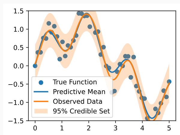
Finally, we plot the fit.

마지막으로 피팅을 플롯합니다.

We see the fits are virtually identical. A few things to note: GPyTorch is working with squared length-scales and observation noise. For example, our learned noise standard deviation in the for scratch code is about 0.283. The noise variance found by GPyTorch is 0.81≈0.2832. In the GPyTorch plot, we also show the credible set in the observation space rather than the latent function space, to demonstrate that they indeed cover the observed datapoints.

우리는 핏이 거의 동일하다는 것을 알 수 있습니다. 몇 가지 참고 사항: GPyTorch는 제곱 길이 척도와 관찰 노이즈를 사용하여 작업합니다. 예를 들어 스크래치 코드에서 학습된 노이즈 표준 편차는 약 0.283입니다. GPyTorch에서 발견한 노이즈 분산은 0.81≒0.2832입니다. GPyTorch 플롯에서는 잠재 함수 공간이 아닌 관찰 공간에 신뢰할 수 있는 세트도 표시하여 실제로 관찰된 데이터 포인트를 포괄한다는 것을 보여줍니다.

18.3.6. Summary

We can combine a Gaussian process prior with data to form a posterior, which we use to make predictions. We can also form a marginal likelihood, which is useful for automatic learning of kernel hyperparameters, which control properties such as the rate of variation of the Gaussian process. The mechanics of forming the posterior and learning kernel hyperparameters for regression are simple, involving about a dozen lines of code. This notebook is a good reference for any reader wanting to quickly get “up and running” with Gaussian processes. We also introduced the GPyTorch library. Although the GPyTorch code for basic regression is relatively long, it can be trivially modified for other kernel functions, or more advanced functionality we will discuss in future notebooks, such as scalable inference, or non-Gaussian likelihoods for classification.

Gaussian process prior 를 데이터와 결합하여 posterior 를 형성하고 이를 예측에 사용할 수 있습니다. 또한 가우스 프로세스의 변동률과 같은 속성을 제어하는 커널 하이퍼파라미터의 자동 학습에 유용한 주변 우도를 형성할 수도 있습니다. 회귀를 위한 사후 및 학습 커널 하이퍼파라미터를 형성하는 메커니즘은 약 12줄의 코드를 포함하여 간단합니다. 이 노트북은 가우스 프로세스를 신속하게 "시작하고 실행"하려는 모든 독자에게 좋은 참고 자료입니다. GPyTorch 라이브러리도 소개했습니다. 기본 회귀를 위한 GPyTorch 코드는 상대적으로 길지만 다른 커널 기능이나 확장 가능한 추론 또는 분류를 위한 비가우시안 가능성과 같은 향후 노트북에서 논의할 고급 기능을 위해 쉽게 수정할 수 있습니다.

18.3.7. Exercises

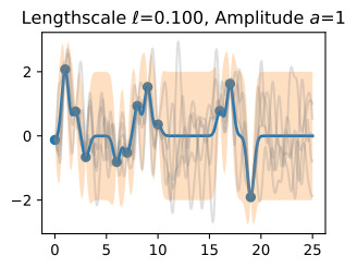
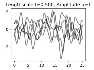
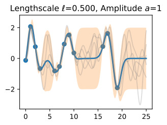
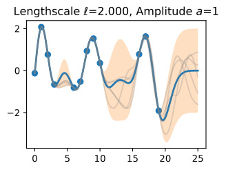
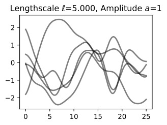
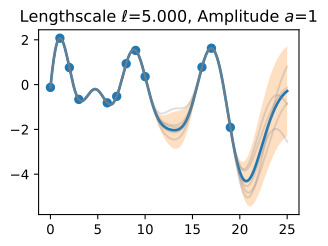
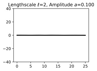
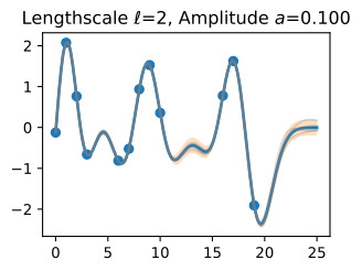
1. We have emphasized the importance of learning kernel hyperparameters, and the effect of hyperparameters and kernels on the generalization properties of Gaussian processes. Try skipping the step where we learn hypers, and instead guess a variety of length-scales and noise variances, and check their effect on predictions. What happens when you use a large length-scale? A small length-scale? A large noise variance? A small noise variance?
2. We have said that the marginal likelihood is not a convex objective, but that hyperparameters like length-scale and noise variance can be reliably estimated in GP regression. This is generally true — in fact, the marginal likelihood is much better at learning length-scale hyperparameters than conventional approaches in spatial statistics, which involve fitting empirical autocorrelation functions (“covariograms”). Arguably, the biggest contribution from machine learning to Gaussian process research, at least before recent work on scalable inference, was the introduction of the marginal lkelihood for hyperparameter learning.

However, different pairings of even these parameters provide interpretably different plausible explanations for many datasets, leading to local optima in our objective. If we use a large length-scale, then we assume the true underlying function is slowly varying. If the observed data are varying significantly, then the only we can plausibly have a large length-scale is with a large noise-variance. If we use a small length-scale, on the other hand, our fit will be very sensitive to the variations in the data, leaving little room to explain variations with noise (aleatoric uncertainty).

Try seeing if you can find these local optima: initialize with very large length-scale with large noise, and small length-scales with small noise. Do you converge to different solutions?

1. We have said that a fundamental advantage of Bayesian methods is in naturally representing epistemic uncertainty. In the above example, we cannot fully see the effects of epistemic uncertainty. Try instead to predict with test_x = np.linspace(0, 10, 1000). What happens to the 95% credible set as your predictions move beyond the data? Does it cover the true function in that interval? What happens if you only visualize aleatoric uncertainty in that region?
2. Try running the above example, but instead with 10,000, 20,000 and 40,000 training points, and measure the runtimes. How does the training time scale? Alternatively, how do the runtimes scale with the number of test points? Is it different for the predictive mean and the predictive variance? Answer this question both by theoretically working out the training and testing time complexities, and by running the code above with a different number of points.
3. Try running the GPyTorch example with different covariance functions, such as the Matern kernel. How do the results change? How about the spectral mixture kernel, found in the GPyTorch library? Are some easier to train the marginal likelihood than others? Are some more valuable for long-range versus short-range predictions?
4. In our GPyTorch example, we plotted the predictive distribution including observation noise, while in our “from scratch” example, we only included epistemic uncertainty. Re-do the GPyTorch example, but this time only plotting epistemic uncertainty, and compare to the from-scratch results. Do the predictive distributions now look the same? (They should.)

18.2. Gaussian Process Priors — Dive into Deep Learning 1.0.3 documentation (d2l.ai)

18.2. Gaussian Process Priors

Understanding Gaussian processes (GPs) is important for reasoning about model construction and generalization, and for achieving state-of-the-art performance in a variety of applications, including active learning, and hyperparameter tuning in deep learning. GPs are everywhere, and it is in our interests to know what they are and how we can use them.

가우시안 프로세스(GP)를 이해하는 것은 모델 구성 및 일반화에 대한 추론과 능동 학습, 딥 러닝의 하이퍼파라미터 조정을 포함한 다양한 애플리케이션에서 최첨단 성능을 달성하는 데 중요합니다. GP는 어디에나 있으며, GP가 무엇인지, 어떻게 사용할 수 있는지 아는 것이 우리의 이익입니다.

In this section, we introduce Gaussian process priors over functions. In the next notebook, we show how to use these priors to do posterior inference and make predictions. The next section can be viewed as “GPs in a nutshell”, quickly giving what you need to apply Gaussian processes in practice.

이 섹션에서는 함수에 대한 Gaussian process priors를 소개를 합니다. 다음 노트북에서는 이러한 priors를 사용하여 사후 추론을 수행하고 예측하는 방법을 보여줍니다. 다음 섹션은 실제로 가우스 프로세스를 적용하는 데 필요한 내용을 빠르게 제공하는 "간단한 GP"로 볼 수 있습니다.

import numpy as np
from scipy.spatial import distance_matrix
from d2l import torch as d2l

d2l.set_figsize()

위의 코드는 Python 프로그램의 일부분이며, 주로 수학적 및 시각화 라이브러리를 사용하여 그림의 크기를 설정하는 목적으로 사용됩니다. 아래는 코드의 각 부분에 대한 설명입니다:

1. import numpy as np: 이 줄은 NumPy 라이브러리를 가져오고, 'np'라는 별칭으로 라이브러리를 사용할 수 있도록 합니다. NumPy는 다차원 배열 및 행렬 연산을 위한 파이썬 라이브러리로, 수치 계산과 관련된 다양한 기능을 제공합니다.
2. from scipy.spatial import distance_matrix: 이 줄은 SciPy 라이브러리에서 distance_matrix 함수를 가져옵니다. distance_matrix 함수는 점들 간의 거리 행렬을 계산하는 데 사용됩니다.
3. from d2l import torch as d2l: 이 줄은 "d2l" 모듈에서 "torch" 모듈을 가져오고, "d2l" 모듈을 "d2l"로 별칭 지정합니다. 이 모듈은 D2L(Data Science for Dummies) 라이브러리의 일부로서, 딥 러닝 및 기계 학습 교육을 위한 유용한 기능과 도구를 제공합니다.
4. d2l.set_figsize(): 이 줄은 D2L 라이브러리의 set_figsize 함수를 호출하여 현재 그림의 크기를 설정합니다. 이 함수는 일반적으로 그림의 크기를 조절하기 위해 사용됩니다.

이 코드 자체는 주로 라이브러리 및 설정을 가져오고 초기화하기 위한 것으로, 여기서는 실제 작업이 수행되지 않습니다. 코드의 나머지 부분이나 주변 문맥에서 더 많은 정보가 필요할 것입니다.

Gaussian Process Prior 란? (GPT 답변)

**가우시안 프로세스 사전(Gaussian Process Prior)**는 가우시안 프로세스(GP) 모델에서 사용되는 중요한 개념 중 하나입니다. GP는 확률적인 회귀 및 분류 문제를 해결하는 데 사용되는 확률적인 모델링 도구 중 하나로, 데이터 포인트 간의 관계를 모델링하는 데 사용됩니다.

가우시안 프로세스 사전은 모델링하려는 함수의 사전 정보 또는 가정을 나타냅니다. 이것은 GP 모델을 어떤 종류의 함수로 가정하고, 모델의 평균 및 공분산 구조를 결정하는 데 사용됩니다. GP 사전은 모델을 더 효과적으로 최적화하고, 모델이 데이터에 더 잘 적합하도록 도울 수 있습니다.

가우시안 프로세스 사전의 주요 요소는 다음과 같습니다:

1. 평균 함수(Mean Function): GP 모델의 평균 함수는 예측 모델이 데이터를 따라 어떻게 중심에 위치해야 하는지를 제시합니다. 평균 함수는 데이터에 따라 조정될 수 있으며, 예측 모델이 평균 함수를 따라 움직입니다.
2. 공분산 함수(Covariance Function 또는 Kernel 함수): GP 모델의 공분산 함수는 데이터 포인트 간의 관계를 모델링합니다. 이 함수는 데이터 포인트 간의 유사성을 측정하며, 두 데이터 포인트 사이의 거리 또는 유사성을 계산합니다. 일반적으로 RBF(Radial Basis Function) 커널, 선형 커널, 다항식 커널 등 다양한 커널 함수가 사용됩니다.
3. 하이퍼파라미터(Hyperparameters): 가우시안 프로세스 사전은 평균 함수와 공분산 함수의 하이퍼파라미터를 포함합니다. 이러한 하이퍼파라미터는 GP 모델을 조정하고 데이터에 맞게 조절하는 데 사용됩니다. 하이퍼파라미터는 최적화 과정을 통해 조정됩니다.

가우시안 프로세스 사전을 설정하는 방법은 모델링하려는 문제에 따라 다르며, 경험과 도메인 지식이 필요한 경우가 많습니다. 올바른 가우시안 프로세스 사전을 선택하면 모델의 성능을 향상시키고, 데이터에 대한 불확실성을 더 정확하게 모델링할 수 있습니다.

18.2.1. Definition

A Gaussian process is defined as a collection of random variables, any finite number of which have a joint Gaussian distribution. If a function f(x) is a Gaussian process, with mean function m(x) and covariance function or kernel k(x,x′), f(x)∼GP(m,k), then any collection of function values queried at any collection of input points x (times, spatial locations, image pixels, etc.), has a joint multivariate Gaussian distribution with mean vector μ and covariance matrix K: f(x1),…,f(xn)∼N(μ,K), where μi=E[f(xi)]=m(xi)  and  Kij= Cov(f(xi),f(xj)) = k(xi,xj).

가우스 프로세스는 임의 변수의 모음으로 정의되며, 임의의 유한한 수는 공동 가우스 분포를 갖습니다. 함수 f(x)가 평균 함수 m(x)와 공분산 함수 또는 커널 k(x,x′), f(x)∼GP(m,k)를 갖는 가우스 프로세스인 경우 함수 값의 모음 임의의 입력 점 x(시간, 공간 위치, 이미지 픽셀 등) 모음에서 쿼리된 값은 평균 벡터 μ 및 공분산 행렬 K를 갖는 결합 다변량 가우스 분포를 갖습니다: f(x1),…,f(xn)∼N( μ,K), 여기서 μi=E[f(xi)]=m(xi)이고 Kij= Cov(f(xi),f(xj)) = k(xi,xj)입니다.

This definition may seem abstract and inaccessible, but Gaussian processes are in fact very simple objects. 

이 정의는 추상적이고 접근하기 어려운 것처럼 보일 수 있지만 가우스 프로세스는 실제로 매우 간단한 개체입니다. 

Any function with w drawn from a Gaussian (normal) distribution, and ϕ being any vector of basis functions, for example ϕ(x)=(1,x,x**2,...,x**d)⊤, is a Gaussian process. Moreover, any Gaussian process f(x) can be expressed in the form of equation (18.2.1). Let’s consider a few concrete examples, to begin getting acquainted with Gaussian processes, after which we can appreciate how simple and useful they really are.

가우스(정규) 분포에서 도출된 w를 갖는 모든 함수, 그리고 ф는 기본 함수의 임의의 벡터입니다. 예를 들어 'ф(x)=(1,x,x**2,...,x**d)⊤'는 가우스 프로세스입니다. 게다가 임의의 가우스 프로세스 f(x)는 방정식 (18.2.1)의 형태로 표현될 수 있습니다. 가우시안 프로세스에 익숙해지기 위해 몇 가지 구체적인 예를 고려해 보겠습니다. 그 후에는 이것이 실제로 얼마나 간단하고 유용한지 평가할 수 있습니다.

18.2.2. A Simple Gaussian Process

Suppose f(x)=w0+w1x, and w0,w1∼N(0,1), with w0,w1,x all in one dimension. We can equivalently write this function as the inner product f(x)=(w0,w1)(1,x)⊤. In (18.2.1) above, w=(w0,w1)**⊤ and ф(x)=(1,x)**⊤.

f(x)=w0+w1x, w0,w1∼N(0,1), w0,w1,x가 모두 1차원에 있다고 가정합니다. 이 함수를 내적 f(x)=(w0,w1)(1,x)⊤로 동등하게 작성할 수 있습니다. 위의 (18.2.1)에서 w=(w0,w1)**⊤ 및 ф(x)=(1,x)**⊤입니다.

For any x, f(x) is a sum of two Gaussian random variables. Since Gaussians are closed under addition, f(x) is also a Gaussian random variable for any x. In fact, we can compute for any particular x that f(x) is N(0,1+x2). Similarly, the joint distribution for any collection of function values, (f(x1),…,f(xn)), for any collection of inputs x1,…,xn, is a multivariate Gaussian distribution. Therefore f(x) is a Gaussian process.

임의의 x에 대해 f(x)는 두 가우스 확률 변수의 합입니다. 가우스는 덧셈에 대해 닫혀 있으므로 f(x)는 모든 x에 대한 가우스 확률 변수이기도 합니다. 실제로, 우리는 f(x)가 N(0,1+x2)인 특정 x에 대해 계산할 수 있습니다. 마찬가지로, 모든 입력 x1,…,xn 컬렉션에 대한 함수 값 컬렉션(f(x1),…,f(xn))에 대한 결합 분포는 다변량 가우스 분포입니다. 따라서 f(x)는 가우스 과정입니다.

In short, f(x) is a random function, or a distribution over functions. We can gain some insights into this distribution by repeatedly sampling values for w0,w1, and visualizing the corresponding functions f(x), which are straight lines with slopes and different intercepts, as follows:

간단히 말해서, f(x)는 무작위 함수, 즉 함수에 대한 분포입니다. 다음과 같이 w0,w1에 대한 값을 반복적으로 샘플링하고 기울기와 다양한 절편이 있는 직선인 해당 함수 f(x)를 시각화하면 이 분포에 대한 통찰력을 얻을 수 있습니다.

def lin_func(x, n_sample):
    preds = np.zeros((n_sample, x.shape[0]))
    for ii in range(n_sample):
        w = np.random.normal(0, 1, 2)
        y = w[0] + w[1] * x
        preds[ii, :] = y
    return preds

x_points = np.linspace(-5, 5, 50)
outs = lin_func(x_points, 10)
lw_bd = -2 * np.sqrt((1 + x_points ** 2))
up_bd = 2 * np.sqrt((1 + x_points ** 2))

d2l.plt.fill_between(x_points, lw_bd, up_bd, alpha=0.25)
d2l.plt.plot(x_points, np.zeros(len(x_points)), linewidth=4, color='black')
d2l.plt.plot(x_points, outs.T)
d2l.plt.xlabel("x", fontsize=20)
d2l.plt.ylabel("f(x)", fontsize=20)
d2l.plt.show()

위의 코드는 주어진 선형 함수를 기반으로 데이터를 생성하고 시각화하는 파이썬 프로그램입니다. 코드의 각 부분에 대한 설명은 다음과 같습니다:

1. def lin_func(x, n_sample):: 이 줄은 lin_func라는 사용자 지정 함수를 정의합니다. 이 함수는 x와 n_sample 두 개의 인자를 받습니다. x는 입력 데이터로 사용되며, n_sample은 데이터 샘플의 수를 나타냅니다.
2. preds = np.zeros((n_sample, x.shape[0])): 이 줄은 결과를 저장할 빈 배열인 preds를 생성합니다. 이 배열은 n_sample개의 행과 x 배열의 길이와 같은 열을 갖습니다.
3. for ii in range(n_sample):: 이 줄은 n_sample만큼 반복하는 루프를 시작합니다.
4. w = np.random.normal(0, 1, 2): 이 줄은 평균이 0이고 표준편차가 1인 정규 분포에서 무작위 가중치 w를 생성합니다. w는 길이가 2인 배열로, 첫 번째 원소는 y 절편을 나타내고 두 번째 원소는 기울기를 나타냅니다.
5. y = w[0] + w[1] * x: 이 줄은 입력 데이터 x에 대한 예측값 y를 계산합니다. 이 예측값은 선형 함수 w[0] + w[1] * x에 의해 생성됩니다.
6. preds[ii, :] = y: 이 줄은 현재 예측값 y를 preds 배열에 저장합니다.
7. return preds: 이 줄은 preds 배열을 반환하고, lin_func 함수를 종료합니다.
8. x_points = np.linspace(-5, 5, 50): 이 줄은 -5부터 5까지의 범위에서 50개의 등간격으로 분포하는 x_points 배열을 생성합니다. 이 배열은 x 값의 범위를 나타냅니다.
9. outs = lin_func(x_points, 10): 이 줄은 앞에서 정의한 lin_func 함수를 호출하여 x_points 값을 사용하여 예측값을 생성합니다. n_sample 매개변수로 10을 전달하므로 10개의 무작위 예측값이 생성됩니다.
10. lw_bd = -2 * np.sqrt((1 + x_points ** 2)) 및 up_bd = 2 * np.sqrt((1 + x_points ** 2)): 이 두 줄은 x_points 값을 사용하여 하한(lw_bd)과 상한(up_bd) 경계를 생성합니다. 이 경계는 시각화에서 사용될 것입니다.
11. d2l.plt.fill_between(x_points, lw_bd, up_bd, alpha=0.25): 이 줄은 fill_between 함수를 사용하여 x_points 범위 내에서 lw_bd와 up_bd 사이를 채우는 영역을 그립니다. alpha 매개변수는 영역의 투명도를 설정합니다.
12. d2l.plt.plot(x_points, np.zeros(len(x_points)), linewidth=4, color='black'): 이 줄은 x 축에 대한 제로 라인을 그리는 것으로, 그림에서 x 축을 나타냅니다.
13. d2l.plt.plot(x_points, outs.T): 이 줄은 outs 배열을 사용하여 x 축에 대한 예측값을 그립니다. 여러 개의 예측값이 그려질 것이며, 각 예측값은 서로 다른 색상으로 표시됩니다.
14. d2l.plt.xlabel("x", fontsize=20) 및 d2l.plt.ylabel("f(x)", fontsize=20): 이 두 줄은 x 축과 y 축에 라벨을 추가하고 글꼴 크기를 설정합니다.
15. d2l.plt.show(): 이 줄은 그림을 화면에 표시합니다.

이 코드는 주어진 선형 함수에 기반하여 데이터를 생성하고 시각적으로 나타내는 데 사용됩니다. 결과 그림에는 선형 함수를 따라 생성된 데이터 포인트와 해당 경계가 표시됩니다.

If w0 and w1 are instead drawn from N(0,a2), how do you imagine varying 'a' affects the distribution over functions?

w0과 w1이 N(0,a2)에서 대신 추출된다면 'a'의 변화가 함수 분포에 어떤 영향을 미칠 것이라고 생각하시나요?

18.2.3. From Weight Space to Function Space

In the plot above, we saw how a distribution over parameters in a model induces a distribution over functions. While we often have ideas about the functions we want to model — whether they’re smooth, periodic, quickly varying, etc. — it is relatively tedious to reason about the parameters, which are largely uninterpretable. Fortunately, Gaussian processes provide an easy mechanism to reason directly about functions. Since a Gaussian distribution is entirely defined by its first two moments, its mean and covariance matrix, a Gaussian process by extension is defined by its mean function and covariance function.

위의 플롯에서 모델의 매개변수에 대한 분포가 함수에 대한 분포를 유도하는 방법을 확인했습니다. 우리는 모델링하려는 함수에 대한 아이디어(매끄럽거나 주기적이거나 빠르게 변화하는 등)에 대해 종종 아이디어를 갖고 있지만 대체로 해석할 수 없는 매개변수에 대해 추론하는 것은 상대적으로 지루합니다. 다행스럽게도 가우스 프로세스는 함수에 대해 직접적으로 추론할 수 있는 쉬운 메커니즘을 제공합니다. 가우스 분포는 처음 두 모멘트인 평균과 공분산 행렬로 완전히 정의되므로 확장에 따른 가우스 프로세스는 평균 함수와 공분산 함수로 정의됩니다.

In the above example, the mean function    위의 예에서 평균 함수는

Similarly, the covariance function is    마찬가지로 공분산 함수는 다음과 같습니다.

Our distribution over functions can now be directly specified and sampled from, without needing to sample from the distribution over parameters. For example, to draw from f(x), we can simply form our multivariate Gaussian distribution associated with any collection of x we want to query, and sample from it directly. We will begin to see just how advantageous this formulation will be.

이제 매개변수에 대한 분포에서 샘플링할 필요 없이 함수에 대한 분포를 직접 지정하고 샘플링할 수 있습니다. 예를 들어 f(x)에서 추출하려면 쿼리하려는 x 컬렉션과 관련된 다변량 가우스 분포를 간단히 구성하고 여기에서 직접 샘플링하면 됩니다. 우리는 이 공식이 얼마나 유리한지 살펴보기 시작할 것입니다.

First, we note that essentially the same derivation for the simple straight line model above can be applied to find the mean and covariance function for any model of the form f(x)=w**⊤ ϕ(x), with w∼N(u,S). In this case, the mean function m(x)=u**⊤ ϕ(x), and the covariance function k(x,x′)=ϕ(x)**⊤ Sϕ(x′). Since ϕ(x) can represent a vector of any non-linear basis functions, we are considering a very general model class, including models with an even an infinite number of parameters.

먼저, 위의 단순 직선 모델에 대해 본질적으로 동일한 파생을 적용하여 'w∼N(u,S)와 함께 f(x)=w**⊤ ф(x) 형식의 모든 모델에 대한 평균 및 공분산 함수를 찾을 수 있습니다.. 이 경우 평균 함수 m(x)=u**⊤ ф(x)이고, 공분산 함수 k(x,x′)=ψ(x)**⊤ Sψ(x′)입니다. ф(x)는 모든 비선형 기저 함수의 벡터를 나타낼 수 있으므로 우리는 무한한 수의 매개변수를 가진 모델을 포함하여 매우 일반적인 모델 클래스를 고려하고 있습니다.

18.2.4. The Radial Basis Function (RBF) Kernel

The radial basis function (RBF) kernel is the most popular covariance function for Gaussian processes, and kernel machines in general. This kernel has the form kRBF(x,x′)=a**2 exp⁡(−1/2ℓ**2||x−x′||2), where 'a' is an amplitude parameter, and ℓ is a lengthscale hyperparameter.

RBF(방사형 기저 함수) 커널은 가우스 프로세스 및 일반적으로 커널 머신에 가장 널리 사용되는 공분산 함수입니다. 이 커널은 kRBF(x,x′)=a**2 exp⁡(−1/2ℓ**2||x−x′||2) 형식을 갖습니다. 여기서 'a'는 진폭 매개변수이고 ℓ는 길이 척도 하이퍼 매개변수입니다.

Radial Basis Function (RBF) Kernel 이란? (GPT3.5 의 답변)

The Radial Basis Function (RBF) kernel, also known as the Gaussian kernel, is a commonly used kernel function in machine learning and statistical modeling. It is particularly popular in the context of Support Vector Machines (SVMs) and Gaussian Processes (GPs).

라디얼 베이시스 함수(Radial Basis Function, RBF) 커널은 기계 학습 및 통계 모델링에서 일반적으로 사용되는 커널 함수로, 특히 서포트 벡터 머신(SVM)과 가우시안 프로세스(GP)의 맥락에서 널리 사용됩니다.

The RBF kernel is defined as: RBF 커널은 다음과 같이 정의됩니다.

K(x, x') = exp(-γ * ||x - x'||^2)

Here, K represents the kernel function, x and x' are data points, ||x - x'|| represents the Euclidean distance between these points, and γ (gamma) is a hyperparameter that controls the kernel's shape. The RBF kernel assigns a similarity or correlation score to pairs of data points based on their distance.

여기서 K는 커널 함수를 나타내며, x와 x'은 데이터 포인트이고, ||x - x'||은 이러한 포인트 간의 유클리드 거리를 나타내며, γ(gamma)는 커널의 모양을 제어하는 하이퍼파라미터입니다. RBF 커널은 데이터 포인트 쌍에 대해 거리를 기반으로 유사성 또는 상관 점수를 할당합니다.

Key characteristics of the RBF kernel include:

RBF 커널의 주요 특징은 다음과 같습니다.

1. Decay with Distance: As the distance between data points increases, the similarity score assigned by the RBF kernel decreases exponentially. This means that nearby points receive higher similarity scores, while distant points receive lower scores.
   
   거리에 따른 감쇠: 데이터 포인트 간 거리가 증가함에 따라 RBF 커널이 할당하는 유사성 점수가 지수적으로 감소합니다. 이것은 가까운 포인트가 더 높은 유사성 점수를 받는 반면 먼 포인트가 더 낮은 점수를 받는다는 것을 의미합니다.
   
   
2. Smoothness: The RBF kernel produces smooth and continuous similarity scores, which makes it suitable for capturing complex patterns and relationships in the data.
   
   부드러움: RBF 커널은 부드럽고 연속적인 유사성 점수를 생성하며, 이로써 데이터의 복잡한 패턴과 관계를 캡처하는 데 적합합니다.
   
   
3. Universal Approximator: The RBF kernel is a universal approximator, meaning it can approximate any continuous function with sufficient data and proper tuning of its hyperparameters.
   
   범용 근사자(Universal Approximator): RBF 커널은 범용 근사자로, 충분한 데이터와 하이퍼파라미터의 적절한 조정을 통해 어떤 연속 함수든 근사화할 수 있습니다.
   
   
4. Hyperparameter γ: The hyperparameter γ controls the "width" of the kernel. Smaller values of γ result in a broader kernel that assigns higher similarity scores to a wider range of data points. Larger values of γ result in a narrower kernel that focuses on closer neighbors.
   
   하이퍼파라미터 γ: 하이퍼파라미터 γ는 커널의 "폭"을 제어합니다. 작은 γ 값은 더 넓은 커널을 생성하여 더 넓은 범위의 데이터 포인트에 높은 유사성 점수를 할당합니다. 큰 γ 값은 더 좁은 커널을 생성하여 더 가까운 이웃에 중점을 둡니다.
   
   

The RBF kernel is often used in various machine learning tasks, such as SVM classification, GP regression, clustering, and dimensionality reduction. It is valued for its ability to capture complex, non-linear relationships in the data, but it may also be sensitive to the choice of the γ hyperparameter, which requires careful tuning for optimal model performance.

RBF 커널은 SVM 분류, GP 회귀, 클러스터링 및 차원 축소와 같은 다양한 기계 학습 작업에서 사용됩니다. 이는 데이터의 복잡한 비선형 관계를 캡처할 수 있는 능력으로 인해 중요하며, 최적의 모델 성능을 위해 γ 하이퍼파라미터 선택에 주의 깊게 조정해야 할 수도 있습니다.

Let’s derive this kernel starting from weight space. Consider the function

가중치 공간에서 시작하여 이 커널을 유도해 보겠습니다. 기능을 고려하십시오

f(x) is a sum of radial basis functions, with width ℓ, centred at the points ci, as shown in the following figure.

f(x)는 다음 그림과 같이 점 ci를 중심으로 너비가 ℓ인 방사형 기저 함수의 합입니다.

We can recognize f(x) as having the form w**⊤ ϕ(x), where w=(w1,…,wJ)**⊤ and ϕ(x) is a vector containing each of the radial basis functions. The covariance function of this Gaussian process is then

f(x)는 w**⊤ ф(x) 형식을 갖는 것으로 인식할 수 있습니다. 여기서 w=(w1,…,wJ)**⊤이고 ф(x)는 각 방사형 기저 함수를 포함하는 벡터입니다. 이 가우스 프로세스의 공분산 함수는 다음과 같습니다.

Now let’s consider what happens as we take the number of parameters (and basis functions) to infinity. Let cJ=log⁡J, c1=−log⁡ J, and ci+1−ci=Δc=2 log⁡J/J, and J→∞. The covariance function becomes the Riemann sum:

이제 매개변수(및 기본 함수)의 수를 무한대로 가져가면 어떤 일이 발생하는지 생각해 보겠습니다. cJ=log⁡J, c1=−log⁡ J, 그리고 ci+1−ci=Δc=2 log⁡J/J, 그리고 J→라고 하자. 공분산 함수는 리만 합계가 됩니다.

By setting c0=−∞ and c∞=∞, we spread the infinitely many basis functions across the whole real line, each a distance Δc→0 apart:

c0=−무한대와 c무한대=무를 설정함으로써 우리는 무한히 많은 기저 함수를 실제 선 전체에 걸쳐 각각 Δc→0 거리만큼 분산시킵니다.

It is worth taking a moment to absorb what we have done here. By moving into the function space representation, we have derived how to represent a model with an infinite number of parameters, using a finite amount of computation. A Gaussian process with an RBF kernel is a universal approximator, capable of representing any continuous function to arbitrary precision. We can intuitively see why from the above derivation. We can collapse each radial basis function to a point mass taking ℓ→0, and give each point mass any height we wish.

여기서 우리가 한 일을 잠시 흡수해 볼 가치가 있습니다. 함수 공간 표현으로 이동하여 유한한 양의 계산을 사용하여 무한한 수의 매개변수가 있는 모델을 표현하는 방법을 도출했습니다. RBF 커널을 사용하는 가우스 프로세스는 모든 연속 함수를 임의의 정밀도로 표현할 수 있는 범용 근사기입니다. 위의 도출을 통해 그 이유를 직관적으로 알 수 있습니다. 각 방사형 기저 함수를 ℓ→0을 취하는 점 질량으로 축소하고 각 점 질량에 원하는 높이를 부여할 수 있습니다.

So a Gaussian process with an RBF kernel is a model with an infinite number of parameters and much more flexibility than any finite neural network. Perhaps all the fuss about overparametrized neural networks is misplaced. As we will see, GPs with RBF kernels do not overfit, and in fact provide especially compelling generalization performance on small datasets. Moreover, the examples in (Zhang et al., 2021), such as the ability to fit images with random labels perfectly, but still generalize well on structured problems, (can be perfectly reproduced using Gaussian processes) (Wilson and Izmailov, 2020). Neural networks are not as distinct as we make them out to be.

따라서 RBF 커널을 사용하는 가우스 프로세스는 무한한 수의 매개 변수와 유한 신경망보다 훨씬 더 많은 유연성을 갖춘 모델입니다. 아마도 과도하게 매개변수화된 신경망에 대한 모든 소란은 잘못된 것일 수도 있습니다. 앞으로 살펴보겠지만 RBF 커널을 사용하는 GP는 과적합되지 않으며 실제로 작은 데이터 세트에서 특히 강력한 일반화 성능을 제공합니다. 더욱이 (Zhang et al., 2021)의 예에서는 임의의 레이블이 있는 이미지를 완벽하게 맞추면서도 구조화된 문제에 대해 여전히 잘 일반화하는 기능과 같은 것입니다(가우시안 프로세스를 사용하여 완벽하게 재현 가능)(Wilson and Izmailov, 2020). . 신경망은 우리가 생각하는 것만큼 뚜렷하지 않습니다.

We can build further intuition about Gaussian processes with RBF kernels, and hyperparameters such as length-scale, by sampling directly from the distribution over functions. As before, this involves a simple procedure:

함수에 대한 분포에서 직접 샘플링함으로써 RBF 커널과 길이 척도와 같은 하이퍼파라미터를 사용하는 가우스 프로세스에 대한 추가 직관을 구축할 수 있습니다. 이전과 마찬가지로 여기에는 간단한 절차가 포함됩니다.

1. Choose the input x points we want to query the GP: x1,…,xn.
   
   GP에 쿼리하려는 입력 x 포인트(x1,…,xn)를 선택합니다.
   
   
2. Evaluate m(xi), i=1,…,n, and k(xi,xj) for i,j=1,…,n to respectively form the mean vector and covariance matrix μ and K, where (f(x1),…,f(xn))∼N(μ,K).
   
   i,j=1,…,n에 대해 m(xi), i=1,…,n 및 k(xi,xj)를 계산하여 각각 평균 벡터와 공분산 행렬 μ 및 K를 형성합니다. 여기서 (f(x1) ,…,f(xn))∼N(μ,K).
   
   
3. Sample from this multivariate Gaussian distribution to obtain the sample function values.
   
   이 다변량 가우스 분포에서 샘플링하여 샘플 함수 값을 얻습니다.
   
   
4. Sample more times to visualize more sample functions queried at those points.
   
   더 많은 횟수를 샘플링하여 해당 지점에서 쿼리된 더 많은 샘플 함수를 시각화합니다.

We illustrate this process in the figure below.

아래 그림에서는 이 프로세스를 설명합니다.

def rbfkernel(x1, x2, ls=4.):  #@save
    dist = distance_matrix(np.expand_dims(x1, 1), np.expand_dims(x2, 1))
    return np.exp(-(1. / ls / 2) * (dist ** 2))

x_points = np.linspace(0, 5, 50)
meanvec = np.zeros(len(x_points))
covmat = rbfkernel(x_points,x_points, 1)

prior_samples= np.random.multivariate_normal(meanvec, covmat, size=5);
d2l.plt.plot(x_points, prior_samples.T, alpha=0.5)
d2l.plt.show()

위의 코드는 라디언 기저 함수(Radial Basis Function, RBF) 커널을 사용하여 가우시안 프로세스(Gaussian Process)의 사전 분포를 시각화하는 파이썬 프로그램입니다. 이 코드를 한 줄씩 설명하겠습니다:

1. def rbfkernel(x1, x2, ls=4.):: 이 줄은 rbfkernel 함수를 정의합니다. 이 함수는 두 개의 입력 x1과 x2를 받고, 추가적인 매개변수로 ls를 받습니다. ls는 커널의 길이 스케일을 나타내는 매개변수로, 기본값은 4입니다.
2. dist = distance_matrix(np.expand_dims(x1, 1), np.expand_dims(x2, 1)): 이 줄은 입력 데이터 x1과 x2 사이의 거리 행렬(dist)을 계산합니다. distance_matrix 함수를 사용하여 x1과 x2 간의 모든 가능한 거리를 계산합니다.
3. return np.exp(-(1. / ls / 2) * (dist ** 2)): 이 줄은 RBF 커널의 계산을 수행합니다. RBF 커널은 가우시안 형태로, 두 데이터 포인트 간의 거리를 지수 함수의 형태로 변환하여 반환합니다. ls는 커널의 길이 스케일을 조절하는 매개변수로, 커널의 폭을 조절합니다.
4. x_points = np.linspace(0, 5, 50): 이 줄은 0부터 5까지의 범위에서 50개의 등간격으로 분포하는 x_points 배열을 생성합니다. 이 배열은 x 값의 범위를 나타냅니다.
5. meanvec = np.zeros(len(x_points)): 이 줄은 x_points와 같은 길이의 제로 벡터인 meanvec를 생성합니다. 이 벡터는 가우시안 프로세스의 평균 벡터로 사용됩니다.
6. covmat = rbfkernel(x_points, x_points, 1): 이 줄은 rbfkernel 함수를 호출하여 x_points에 대한 공분산 행렬(covmat)을 계산합니다. 이 공분산 행렬은 RBF 커널을 사용하여 생성되며, ls 매개변수의 값이 1로 설정되어 있습니다.
7. prior_samples = np.random.multivariate_normal(meanvec, covmat, size=5): 이 줄은 meanvec와 covmat을 사용하여 가우시안 분포에서 5개의 무작위 샘플(prior_samples)을 생성합니다. 이 샘플은 가우시안 프로세스의 사전 분포에서 추출된 것입니다.
8. d2l.plt.plot(x_points, prior_samples.T, alpha=0.5): 이 줄은 prior_samples를 시각화합니다. 각각의 무작위 샘플은 x_points에 대해 그래프로 표시되며, alpha 매개변수를 사용하여 투명도를 설정합니다.
9. d2l.plt.show(): 이 줄은 그래프를 화면에 표시합니다.

이 코드는 가우시안 프로세스의 사전 분포를 시각화하기 위해 RBF 커널을 사용하는 간단한 예제를 제공합니다. 이를 통해 가우시안 프로세스가 어떻게 작동하는지 이해할 수 있습니다.

18.2.5. The Neural Network Kernel

Research on Gaussian processes in machine learning was triggered by research on neural networks. Radford Neal was pursuing ever larger Bayesian neural networks, ultimately showing in 1994 (later published in 1996, as it was one of the most infamous NeurIPS rejections) that such networks with an infinite number of hidden units become Gaussian processes with particular kernel functions (Neal, 1996). Interest in this derivation has re-surfaced, with ideas like the neural tangent kernel being used to investigate the generalization properties of neural networks (Matthews et al., 2018) (Novak et al., 2018). We can derive the neural network kernel as follows.

기계 학습의 가우스 프로세스에 대한 연구는 신경망에 대한 연구에서 시작되었습니다. Radford Neal은 훨씬 더 큰 베이지안 신경망을 추구했으며, 궁극적으로 1994년에(나중에 가장 악명 높은 NeurIPS 거부 중 하나인 1996년에 출판됨) 무한한 수의 숨겨진 단위를 가진 그러한 네트워크가 특정 커널 기능을 가진 가우스 프로세스가 된다는 것을 보여주었습니다(Neal , 1996). 신경망의 일반화 속성을 조사하는 데 신경 접선 커널과 같은 아이디어가 사용되면서 이 파생에 대한 관심이 다시 표면화되었습니다(Matthews et al., 2018)(Novak et al., 2018). 신경망 커널은 다음과 같이 유도할 수 있습니다.

Consider a neural network function f(x) with one hidden layer:

하나의 은닉층이 있는 신경망 함수 f(x)를 생각해 보세요.

b is a bias, vi are the hidden to output weights, ℎ is any bounded hidden unit transfer function, ui are the input to hidden weights, and J is the number of hidden units. Let b and vi be independent with zero mean and variances σ**2 b and σ**2v/J, respectively, and let the ui have independent identical distributions. We can then use the central limit theorem to show that any collection of function values f(x1),…,f(xn) has a joint multivariate Gaussian distribution.

b는 편향, vi는 출력 가중치에 대한 은닉, ℎ는 경계가 있는 숨겨진 단위 전달 함수, ui는 숨겨진 가중치에 대한 입력, J는 숨겨진 단위의 수입니다. b와 vi가 평균이 0이고 분산이 각각 σ**2 b 및 σ**2v/J인 독립이고 ui가 독립적인 동일한 분포를 갖는다고 가정합니다. 그런 다음 중심 극한 정리를 사용하여 함수 값 f(x1),…,f(xn)의 집합이 결합 다변량 가우스 분포를 가짐을 보여줄 수 있습니다.

The mean and covariance function of the corresponding Gaussian process are:

해당 가우스 프로세스의 평균 및 공분산 함수는 다음과 같습니다.

In some cases, we can essentially evaluate this covariance function in closed form. Let ℎ(x;u)=erf(u0+∑**p j=1 ujxj), where

The RBF kernel is stationary, meaning that it is translation invariant, and therefore can be written as a function of T=x−x′. Intuitively, stationarity means that the high-level properties of the function, such as rate of variation, do not change as we move in input space. The neural network kernel, however, is non-stationary. Below, we show sample functions from a Gaussian process with this kernel. We can see that the function looks qualitatively different near the origin.

RBF 커널은 고정적입니다. 즉, 변환 불변이므로 T=x−x′의 함수로 작성할 수 있습니다. 직관적으로 정상성은 입력 공간에서 이동할 때 변동률과 같은 함수의 상위 수준 속성이 변경되지 않음을 의미합니다. 그러나 신경망 커널은 고정되어 있지 않습니다. 아래에서는 이 커널을 사용한 가우스 프로세스의 샘플 함수를 보여줍니다. 함수가 원점 근처에서 질적으로 다르게 보이는 것을 볼 수 있습니다.

18.2.6. Summary

The first step in performing Bayesian inference involves specifying a prior. Gaussian processes can be used to specify a whole prior over functions. Starting from a traditional “weight space” view of modelling, we can induce a prior over functions by starting with the functional form of a model, and introducing a distribution over its parameters. We can alternatively specify a prior distribution directly in function space, with properties controlled by a kernel. The function-space approach has many advantages. We can build models that actually correspond to an infinite number of parameters, but use a finite amount of computation! Moreover, while these models have a great amount of flexibility, they also make strong assumptions about what types of functions are a priori likely, leading to relatively good generalization on small datasets.

베이지안 추론을 수행하는 첫 번째 단계는 사전 지정을 포함합니다. 가우스 프로세스를 사용하여 함수보다 전체 prior 을 지정할 수 있습니다. 모델링의 전통적인 "가중치 공간" 관점에서 시작하여 모델의 기능적 형태로 시작하고 해당 매개변수에 대한 분포를 도입함으로써 기능에 대한 사전 예측을 유도할 수 있습니다. 또는 커널에 의해 제어되는 속성을 사용하여 함수 공간에서 직접 사전 분포를 지정할 수도 있습니다. 기능 공간 접근 방식에는 많은 장점이 있습니다. 실제로 무한한 수의 매개변수에 해당하는 모델을 구축할 수 있지만 계산량은 한정되어 있습니다. 더욱이 이러한 모델은 상당한 유연성을 갖고 있지만 어떤 유형의 함수가 선험적으로 발생할 가능성이 있는지에 대한 강력한 가정을 만들어 소규모 데이터 세트에 대해 상대적으로 좋은 일반화를 이끌어냅니다.

The assumptions of models in function space are intuitively controlled by kernels, which often encode higher level properties of functions, such as smoothness and periodicity. Many kernels are stationary, meaning that they are translation invariant. Functions drawn from a Gaussian process with a stationary kernel have roughly the same high-level properties (such as rate of variation) regardless of where we look in the input space.

함수 공간에서 모델의 가정은 커널에 의해 직관적으로 제어되며, 커널은 부드러움 및 주기성과 같은 함수의 더 높은 수준 속성을 인코딩하는 경우가 많습니다. 많은 커널은 고정되어 있습니다. 즉, 변환 불변성을 의미합니다. 고정 커널을 사용하는 가우스 프로세스에서 도출된 함수는 입력 공간에서 보는 위치에 관계없이 대략 동일한 높은 수준의 속성(예: 변동률)을 갖습니다.

Gaussian processes are a relatively general model class, containing many examples of models we are already familiar with, including polynomials, Fourier series, and so on, as long as we have a Gaussian prior over the parameters. They also include neural networks with an infinite number of parameters, even without Gaussian distributions over the parameters. This connection, discovered by Radford Neal, triggered machine learning researchers to move away from neural networks, and towards Gaussian processes.

가우스 프로세스는 매개변수에 대한 가우스 사전이 있는 한 다항식, 푸리에 급수 등을 포함하여 우리에게 이미 익숙한 모델의 많은 예를 포함하는 비교적 일반적인 모델 클래스입니다. 또한 매개변수에 대한 가우스 분포가 없더라도 매개변수 수가 무한한 신경망도 포함됩니다. Radford Neal이 발견한 이 연결은 기계 학습 연구자들이 신경망에서 벗어나 가우스 프로세스로 이동하도록 촉발했습니다.

18.2.7. Exercises

18.1. Introduction to Gaussian Processes — Dive into Deep Learning 1.0.3 documentation (d2l.ai)

18.1. Introduction to Gaussian Processes

Let’s get a feel for how Gaussian processes operate, by starting with some examples.

몇 가지 예를 통해 가우스 프로세스가 어떻게 작동하는지 살펴보겠습니다.

Suppose we observe the following dataset, of regression targets (outputs), y, indexed by inputs, x. As an example, the targets could be changes in carbon dioxide concentrations, and the inputs could be the times at which these targets have been recorded. What are some features of the data? How quickly does it seem to varying? Do we have data points collected at regular intervals, or are there missing inputs? How would you imagine filling in the missing regions, or forecasting up until x=25?

입력 x로 인덱싱된 회귀 목표(출력) y의 다음 데이터 세트를 관찰한다고 가정합니다. 예를 들어 목표는 이산화탄소 농도의 변화일 수 있고 입력은 이러한 목표가 기록된 시간일 수 있습니다. 데이터의 일부 기능은 무엇입니까? 얼마나 빨리 변하는 것 같나요? 정기적으로 수집된 데이터 포인트가 있습니까, 아니면 누락된 입력이 있습니까? 누락된 영역을 채우거나 x=25까지 예측하는 것을 어떻게 상상하시겠습니까?

In order to fit the data with a Gaussian process, we start by specifying a prior distribution over what types of functions we might believe to be reasonable. Here we show several sample functions from a Gaussian process. Does this prior look reasonable? Note here we are not looking for functions that fit our dataset, but instead for specifying reasonable high-level properties of the solutions, such as how quickly they vary with inputs. Note that we will see code for reproducing all of the plots in this notebook, in the next notebooks on priors and inference.

데이터를 가우스 프로세스에 맞추려면 합리적이라고 믿을 수 있는 함수 유형에 대한 사전 분포를 지정하는 것부터 시작합니다. 여기서는 가우스 프로세스의 몇 가지 샘플 함수를 보여줍니다. 이 사전 조치가 합리적으로 보입니까? 여기서는 데이터 세트에 맞는 함수를 찾는 것이 아니라 입력에 따라 얼마나 빨리 변하는 지와 같은 솔루션의 합리적인 상위 수준 속성을 지정하기 위한 것입니다. 사전 및 추론에 대한 다음 노트북에서 이 노트북의 모든 플롯을 재현하기 위한 코드를 볼 수 있습니다.

Once we condition on data, we can use this prior to infer a posterior distribution over functions that could fit the data. Here we show sample posterior functions.

데이터에 조건을 적용하면 데이터에 적합한 함수에 대한 사후 분포를 추론하기 전에 이를 사용할 수 있습니다. 여기서는 샘플 사후 함수를 보여줍니다.

We see that each of these functions are entirely consistent with our data, perfectly running through each observation. In order to use these posterior samples to make predictions, we can average the values of every possible sample function from the posterior, to create the curve below, in thick blue. Note that we do not actually have to take an infinite number of samples to compute this expectation; as we will see later, we can compute the expectation in closed form.

우리는 이러한 각 함수가 데이터와 완전히 일치하며 각 관찰을 통해 완벽하게 실행된다는 것을 알 수 있습니다. 예측을 위해 이러한 사후 샘플을 사용하기 위해 사후에서 가능한 모든 샘플 함수의 값을 평균화하여 아래 곡선을 두꺼운 파란색으로 만들 수 있습니다. 이 기대치를 계산하기 위해 실제로 무한한 수의 샘플을 취할 필요는 없습니다. 나중에 살펴보겠지만 닫힌 형식으로 기대값을 계산할 수 있습니다.

We may also want a representation of uncertainty, so we know how confident we should be in our predictions. Intuitively, we should have more uncertainty where there is more variability in the sample posterior functions, as this tells us there are many more possible values the true function could take. This type of uncertainty is called epistemic uncertainty, which is the reducible uncertainty associated with lack of information. As we acquire more data, this type of uncertainty disappears, as there will be increasingly fewer solutions consistent with what we observe. Like with the posterior mean, we can compute the posterior variance (the variability of these functions in the posterior) in closed form. With shade, we show two times the posterior standard deviation on either side of the mean, creating a credible interval that has a 95% probability of containing the true value of the function for any input x.

우리는 불확실성을 표현하기를 원할 수도 있으므로 예측에 얼마나 자신감을 가져야 하는지 알 수 있습니다. 직관적으로, 표본 사후 함수에 변동성이 더 많을수록 불확실성이 커집니다. 이는 실제 함수가 취할 수 있는 가능한 값이 더 많다는 것을 의미하기 때문입니다. 이러한 유형의 불확실성을 인식론적 불확실성이라고 하며, 이는 정보 부족과 관련된 환원 가능한 불확실성입니다. 더 많은 데이터를 수집할수록 우리가 관찰한 것과 일치하는 솔루션이 점점 줄어들기 때문에 이러한 유형의 불확실성은 사라집니다. 사후 평균과 마찬가지로 사후 분산(후방에서 이러한 함수의 변동성)을 닫힌 형식으로 계산할 수 있습니다. 음영을 사용하면 평균의 양쪽에 사후 표준 편차의 두 배를 표시하여 입력 x에 대한 함수의 실제 값을 포함할 확률이 95%인 신뢰할 수 있는 구간을 만듭니다.

The plot looks somewhat cleaner if we remove the posterior samples, simply visualizing the data, posterior mean, and 95% credible set. Notice how the uncertainty grows away from the data, a property of epistemic uncertainty.

사후 샘플을 제거하고 데이터, 사후 평균 및 95% 신뢰 세트를 시각화하면 플롯이 다소 더 깨끗해 보입니다. 인식론적 불확실성의 속성인 불확실성이 데이터에서 어떻게 멀어지는지 주목하세요.

The properties of the Gaussian process that we used to fit the data are strongly controlled by what’s called a covariance function, also known as a kernel. The covariance function we used is called the RBF (Radial Basis Function) kernel, which has the form

데이터를 맞추는 데 사용한 가우스 프로세스의 속성은 커널이라고도 알려진 공분산 함수에 의해 강력하게 제어됩니다. 우리가 사용한 공분산 함수는 RBF(방사형 기초 함수) 커널이라고 하며 다음과 같은 형식을 갖습니다.

공분산 함수 (Covariance function) 란?

Covariance function (also known as a kernel function in machine learning) is a mathematical function used in statistics and machine learning to quantify the degree to which two random variables (or data points) vary together. It provides a measure of how correlated or related two variables are to each other.

공분산 함수 (머신 러닝에서는 커널 함수로도 알려져 있음)는 통계 및 머신 러닝에서 두 개의 랜덤 변수(또는 데이터 포인트)가 함께 얼마나 변하는지를 측정하는 수학적 함수입니다. 이것은 두 변수가 서로 어떻게 상관되거나 관련되어 있는지를 측정하는 데 사용됩니다.

In the context of statistics and Gaussian processes, the covariance function specifies the relationship between different points in a dataset. It defines how the value of one data point covaries or varies with the value of another data point. This information is crucial for modeling and understanding the underlying patterns and relationships within the data.

Covariance functions are often used in:

통계 및 가우시안 프로세스의 맥락에서 공분산 함수는 데이터 집합의 서로 다른 지점 간의 관계를 지정합니다. 이것은 하나의 데이터 포인트의 값이 다른 데이터 포인트의 값과 어떻게 공분산하거나 변하는지를 정의합니다. 이 정보는 데이터 내부의 기본적인 패턴과 관계를 모델링하고 이해하는 데 중요합니다.

공분산 함수는 다음과 같은 분야에서 사용됩니다.

1. Gaussian Processes: In Gaussian processes, the covariance function (kernel) is a fundamental component. It determines how the values of the function being modeled vary across different input points. Common covariance functions include the Radial Basis Function (RBF) kernel, Matérn kernel, and many others.
   
   가우시안 프로세스: 가우시안 프로세스에서 공분산 함수(커널)는 기본 구성 요소입니다. 이것은 모델링하려는 함수의 값이 다른 입력 지점에서 어떻게 변하는지를 결정합니다. 일반적인 공분산 함수에는 방사형 기저 함수(RBF) 커널, Matérn 커널 및 기타 여러 가지가 있습니다.
   
   
2. Spatial Statistics: In geostatistics and spatial statistics, covariance functions are used to model spatial dependencies in data, such as the correlation between temperatures at different locations on a map.
   
   공간 통계: 지오통계 및 공간 통계에서 공분산 함수는 데이터 내에서 공간적 종속성(지도상의 다른 위치에서 온도 간의 상관 관계와 같은)을 모델링하는 데 사용됩니다.
   
   
3. Machine Learning: In machine learning, covariance functions are used in various algorithms, especially in kernel methods, including Support Vector Machines (SVMs) and Gaussian Process Regression (GPR).
   
   머신 러닝: 머신 러닝에서 공분산 함수는 서포트 벡터 머신(SVM) 및 가우시안 프로세스 회귀(GPR)를 포함한 다양한 알고리즘에서 사용됩니다.
   
   

The choice of covariance function or kernel function has a significant impact on the performance of a model. Different covariance functions capture different types of relationships in the data, such as smoothness, periodicity, or linearity. Adjusting the parameters of the covariance function allows for fine-tuning the model's behavior.

공분산 함수 또는 커널 함수의 선택은 모델의 성능에 큰 영향을 미칩니다. 서로 다른 공분산 함수는 데이터에서 서로 다른 유형의 관계(부드러움, 주기성, 직선성 등)를 포착하며 공분산 함수의 매개변수를 조정하면 모델의 동작을 세밀하게 조정할 수 있습니다.

The hyperparameters of this kernel are interpretable. The amplitude parameter 'a' controls the vertical scale over which the function is varying, and the length-scale parameter ℓ controls the rate of variation (the wiggliness) of the function. Larger 'a' means larger function values, and larger ℓ means more slowly varying functions. Let’s see what happens to our sample prior and posterior functions as we vary 'a' and ℓ.

이 커널의 하이퍼파라미터는 해석 가능합니다. 진폭 매개변수 'a'는 함수가 변하는 수직 스케일을 제어하고, 길이 스케일 매개변수 ℓ는 함수의 변동률(흔들림)을 제어합니다. 'a'가 클수록 함수 값이 크고, ℓ가 클수록 함수가 천천히 변한다는 의미입니다. 'a'와 ℓ를 변경하면 샘플 사전 및 사후 함수에 어떤 일이 발생하는지 살펴보겠습니다.

The length-scale has a particularly pronounced effect on the predictions and uncertainty of a GP. At ||x−x′||=ℓ , the covariance between a pair of function values is a**2exp⁡(−0.5). At larger distances than ℓ , the values of the function values becomes nearly uncorrelated. This means that if we want to make a prediction at a point x∗, then function values with inputs x such that ||x−x′||>ℓ will not have a strong effect on our predictions.

길이 척도는 GP의 예측과 불확실성에 특히 뚜렷한 영향을 미칩니다. ||x−x′||=ℓ 에서 함수 값 쌍 사이의 공분산은 a**2exp⁡(−0.5)입니다. ℓ 보다 큰 거리에서는 함수 값의 상관관계가 거의 없어집니다. 이는 x* 지점에서 예측을 수행하려는 경우 ||x−x′||>ℓ와 같은 입력 x가 있는 함수 값이 예측에 큰 영향을 미치지 않음을 의미합니다.

Let’s see how changing the lengthscale affects sample prior and posterior functions, and credible sets. The above fits use a length-scale of 2. Let’s now consider ℓ=0.1,0.5,2,5,10 . A length-scale of 0.1 is very small relative to the range of the input domain we are considering, 25. For example, the values of the function at x=5 and x=10 will have essentially no correlation at such a length-scale. On the other hand, for a length-scale of 10, the function values at these inputs will be highly correlated. Note that the vertical scale changes in the following figures.

길이 척도를 변경하면 샘플 사전 및 사후 함수와 신뢰할 수 있는 세트에 어떤 영향을 미치는지 살펴보겠습니다. 위의 피팅은 길이 척도 2를 사용합니다. 이제 ℓ=0.1,0.5,2,5,10을 고려해 보겠습니다. 0.1의 길이 척도는 우리가 고려하고 있는 입력 영역의 범위인 25에 비해 매우 작습니다. 예를 들어 x=5와 x=10의 함수 값은 이러한 길이 척도에서 본질적으로 상관 관계가 없습니다. . 반면, 길이 척도가 10인 경우 이러한 입력의 함수 값은 높은 상관 관계를 갖습니다. 다음 그림에서는 수직 스케일이 변경됩니다.

Notice as the length-scale increases the ‘wiggliness’ of the functions decrease, and our uncertainty decreases. If the length-scale is small, the uncertainty will quickly increase as we move away from the data, as the datapoints become less informative about the function values.

길이 척도가 증가함에 따라 함수의 '흔들림'이 감소하고 불확실성이 감소합니다. 길이 척도가 작으면 데이터 포인트가 함수 값에 대한 정보를 덜 제공하므로 데이터에서 멀어질수록 불확실성이 빠르게 증가합니다.

Now, let’s vary the amplitude parameter, holding the length-scale fixed at 2. Note the vertical scale is held fixed for the prior samples, and varies for the posterior samples, so you can clearly see both the increasing scale of the function, and the fits to the data.

이제 길이 스케일을 2로 고정하여 진폭 매개변수를 변경해 보겠습니다. 수직 스케일은 이전 샘플에 대해 고정되어 있고 사후 샘플에 대해 달라집니다. 따라서 함수의 스케일 증가와 데이터에 적합합니다.

We see the amplitude parameter affects the scale of the function, but not the rate of variation. At this point, we also have the sense that the generalization performance of our procedure will depend on having reasonable values for these hyperparameters. Values of ℓ=2 and a=1 appeared to provide reasonable fits, while some of the other values did not. Fortunately, there is a robust and automatic way to specify these hyperparameters, using what is called the marginal likelihood, which we will return to in the notebook on inference.

진폭 매개변수는 함수의 규모에 영향을 주지만 변동률에는 영향을 미치지 않습니다. 이 시점에서 우리는 프로시저의 일반화 성능이 이러한 하이퍼파라미터에 대한 합리적인 값을 갖는지에 달려 있다는 것을 알게 되었습니다. ℓ=2 및 a=1 값은 합리적인 적합치를 제공하는 것으로 보였지만 일부 다른 값은 그렇지 않았습니다. 다행스럽게도 한계 우도(Marginal Likelihood)를 사용하여 이러한 하이퍼파라미터를 지정하는 강력하고 자동적인 방법이 있습니다. 이 방법은 추론에 대한 노트북에서 다시 설명하겠습니다.

So what is a GP, really? As we started, a GP simply says that any collection of function values f(x1),…,f(xn), indexed by any collection of inputs x1,…,xn has a joint multivariate Gaussian distribution. The mean vector μ of this distribution is given by a mean function, which is typically taken to be a constant or zero. The covariance matrix of this distribution is given by the kernel evaluated at all pairs of the inputs x.

그렇다면 GP란 무엇일까요? 우리가 시작했을 때, GP는 단순히 입력 x1,…,xn의 컬렉션에 의해 인덱스된 함수 값 f(x1),…,f(xn)의 컬렉션이 결합 다변량 가우스 분포를 갖는다고 말합니다. 이 분포의 평균 벡터 μ는 평균 함수로 제공되며 일반적으로 상수 또는 0으로 간주됩니다. 이 분포의 공분산 행렬은 모든 입력 x 쌍에서 평가된 커널에 의해 제공됩니다.

Equation (18.1.2) specifies a GP prior. We can compute the conditional distribution of f(x) for any x given f(x1),…,f(xn), the function values we have observed. This conditional distribution is called the posterior, and it is what we use to make predictions.

식 (18.1.2)은 GP 사전을 지정합니다. 우리가 관찰한 함수 값 f(x1),…,f(xn)이 주어지면 임의의 x에 대해 f(x)의 조건부 분포를 계산할 수 있습니다. 이 조건부 분포를 사후 분포라고 하며 예측을 위해 사용합니다.

In particular,  특히,

where k(x,x1:n) is a 1×n vector formed by evaluating k(x,xi) for i=1,…,n and k(x1:n,x1:n) is an n×n matrix formed by evaluating k(xi,xj) for i,j=1,…,n. m is what we can use as a point predictor for any x, and s**2 is what we use for uncertainty: if we want to create an interval with a 95% probability that f(x) is in the interval, we would use m±2s. The predictive means and uncertainties for all the above figures were created using these equations. The observed data points were given by f(x1),…,f(xn) and chose a fine grained set of x points to make predictions.

여기서 k(x,x1:n)은 i=1,…,n에 대해 k(x,xi)를 평가하여 형성된 1×n 벡터이고 k(x1:n,x1:n)은 형성된 n×n 행렬입니다. i,j=1,…,n에 대해 k(xi,xj)를 평가합니다. m은 임의의 x에 대한 점 예측자로 사용할 수 있는 것이고, s**2는 불확실성에 사용하는 것입니다. f(x)가 구간에 있을 확률이 95%인 구간을 생성하려면 다음과 같이 합니다. m±2초를 사용하세요. 위의 모든 수치에 대한 예측 평균과 불확실성은 이러한 방정식을 사용하여 생성되었습니다. 관찰된 데이터 포인트는 f(x1),…,f(xn)으로 제공되었으며 예측을 위해 세밀한 x 포인트 세트를 선택했습니다.

Let’s suppose we observe a single datapoint, f(x1), and we want to determine the value of f(x) at some x. Because f(x) is described by a Gaussian process, we know the joint distribution over (f(x),f(x1)) is Gaussian:

단일 데이터 포인트 f(x1)를 관찰하고 일부 x에서 f(x)의 값을 결정한다고 가정해 보겠습니다. f(x)는 가우스 프로세스로 설명되므로 (f(x),f(x1))에 대한 결합 분포가 가우스임을 알 수 있습니다.

The off-diagonal expression k(x,x1)=k(x1,x) tells us how correlated the function values will be — how strongly determined f(x) will be from f(x1). We have seen already that if we use a large length-scale, relative to the distance between x and x1, ||x−x1||, then the function values will be highly correlated. We can visualize the process of determining f(x) from f(x1) both in the space of functions, and in the joint distribution over f(x1),f(x). Let’s initially consider an x such that k(x,x1)=0.9, and k(x,x)=1, meaning that the value of f(x) is moderately correlated with the value of f(x1). In the joint distribution, the contours of constant probability will be relatively narrow ellipses.

비대각선 표현식 k(x,x1)=k(x1,x)는 함수 값의 상관 관계, 즉 f(x)가 f(x1)에서 얼마나 강력하게 결정되는지 알려줍니다. 우리는 x와 x1 사이의 거리(||x−x1||)에 상대적으로 큰 길이 척도를 사용하면 함수 값의 상관 관계가 높다는 것을 이미 확인했습니다. 함수 공간과 f(x1),f(x)에 대한 결합 분포 모두에서 f(x1)에서 f(x)를 결정하는 프로세스를 시각화할 수 있습니다. 처음에 k(x,x1)=0.9, k(x,x)=1인 x를 고려해 보겠습니다. 이는 f(x) 값이 f(x1) 값과 중간 정도의 상관 관계가 있음을 의미합니다. 결합 분포에서 일정한 확률의 윤곽은 상대적으로 좁은 타원이 됩니다.

Suppose we observe f(x1)=1.2. To condition on this value of f(x1), we can draw a horizontal line at 1.2 on our plot of the density, and see that the value of f(x) is mostly constrained to [0.64,1.52]. We have also drawn this plot in function space, showing the observed point f(x1) in orange, and 1 standard deviation of the Gaussian process predictive distribution for f(x) in blue, about the mean value of 1.08.

f(x1)=1.2를 관찰한다고 가정합니다. 이 f(x1) 값을 조건으로 하기 위해 밀도 플롯에서 1.2에 수평선을 그릴 수 있으며 f(x) 값이 대부분 [0.64,1.52]로 제한되어 있음을 알 수 있습니다. 우리는 또한 이 플롯을 함수 공간에 그려서 관찰된 점 f(x1)을 주황색으로 표시하고 f(x)에 대한 가우스 프로세스 예측 분포의 1 표준 편차를 파란색으로 표시했습니다(평균값 약 1.08).

Now suppose we have a stronger correlation, k(x,x1)=0.95. Now the ellipses have narrowed further, and the value of f(x) is even more strongly determined by f(x1). Drawing a horizontal line at 1.2, we see the contours for f(x) support values mostly within [0.83,1.45]. Again, we also show the plot in function space, with one standard deviation about the mean predictive value of 1.14.

이제 k(x,x1)=0.95라는 더 강한 상관관계가 있다고 가정합니다. 이제 타원은 더 좁아졌고 f(x)의 값은 f(x1)에 의해 훨씬 더 강력하게 결정됩니다. 1.2에서 수평선을 그리면 f(x) 지원 값의 윤곽이 대부분 [0.83,1.45] 내에 있는 것을 볼 수 있습니다. 다시 말하지만, 평균 예측 값 1.14에 대한 표준 편차가 1인 함수 공간의 플롯도 표시됩니다.

We see that the posterior mean predictor of our Gaussian process is closer to 1.2, because there is now a stronger correlation. We also see that our uncertainty (the error bars) have somewhat decreased. Despite the strong correlation between these function values, our uncertainty is still righly quite large, because we have only observed a single data point!

이제 더 강한 상관관계가 있기 때문에 가우스 프로세스의 사후 평균 예측 변수가 1.2에 더 가깝다는 것을 알 수 있습니다. 또한 불확실성(오차 막대)이 다소 감소한 것을 볼 수 있습니다. 이러한 함수 값 사이의 강한 상관 관계에도 불구하고 우리는 단 하나의 데이터 포인트만 관찰했기 때문에 불확실성은 여전히 상당히 큽니다!

This procedure can give us a posterior on f(x) for any x, for any number of points we have observed. Suppose we observe f(x1),f(x2). We now visualize the posterior for f(x) at a particular x=x′ in function space. The exact distribution for f(x) is given by the above equations. f(x) is Gaussian distributed, with mean

이 절차는 우리가 관찰한 임의의 수의 점에 대해 임의의 x에 대한 f(x)의 사후값을 제공할 수 있습니다. f(x1),f(x2)를 관찰한다고 가정합니다. 이제 함수 공간의 특정 x=x′에서 f(x)의 사후를 시각화합니다. f(x)의 정확한 분포는 위 방정식으로 제공됩니다. f(x)는 평균을 갖는 가우스 분포입니다.

and variance  및 분산

In this introductory notebook, we have been considering noise free observations. As we will see, it is easy to include observation noise. If we assume that the data are generated from a latent noise free function f(x) plus iid Gaussian noise ϵ(x)∼N(0,σ**2) with variance σ**2, then our covariance function simply becomes k(xi,xj)→k(xi,xj)+δijσ**2, where δif=1 if i=j and 0 otherwise.

이 소개 노트에서는 잡음 없는 관찰을 고려했습니다. 앞으로 살펴보겠지만 관찰 노이즈를 포함하는 것은 쉽습니다. 데이터가 잠재 잡음 없는 함수 f(x)와 분산 σ**2를 갖는 iid 가우스 잡음 ϵ(x)∼N(0,σ**2)에서 생성된다고 가정하면 공분산 함수는 간단히 k가 됩니다. (xi,xj)→k(xi,xj)+δijσ**2, 여기서 i=j이면 δif=1이고 그렇지 않으면 0입니다.

We have already started getting some intuition about how we can use a Gaussian process to specify a prior and posterior over solutions, and how the kernel function affects the properties of these solutions. In the following notebooks, we will precisely show how to specify a Gaussian process prior, introduce and derive various kernel functions, and then go through the mechanics of how to automatically learn kernel hyperparameters, and form a Gaussian process posterior to make predictions. While it takes time and practice to get used to concepts such as a “distributions over functions”, the actual mechanics of finding the GP predictive equations is actually quite simple — making it easy to get practice to form an intuitive understanding of these concepts.

우리는 이미 가우스 프로세스를 사용하여 솔루션에 대한 사전 및 사후를 지정하는 방법과 커널 기능이 이러한 솔루션의 속성에 어떻게 영향을 미치는지에 대한 직관을 얻기 시작했습니다. 다음 노트에서는 사전에 가우스 프로세스를 지정하는 방법, 다양한 커널 함수를 소개 및 도출하는 방법, 그리고 커널 하이퍼파라미터를 자동으로 학습하는 방법, 사후에 가우스 프로세스를 형성하여 예측하는 방법에 대한 메커니즘을 자세히 보여줍니다. "함수에 대한 분포"와 같은 개념에 익숙해지려면 시간과 연습이 필요하지만 GP 예측 방정식을 찾는 실제 메커니즘은 실제로 매우 간단하므로 이러한 개념을 직관적으로 이해하기 위한 연습을 쉽게 할 수 있습니다.

18.1.1. Summary

In typical machine learning, we specify a function with some free parameters (such as a neural network and its weights), and we focus on estimating those parameters, which may not be interpretable. With a Gaussian process, we instead reason about distributions over functions directly, which enables us to reason about the high-level properties of the solutions. These properties are controlled by a covariance function (kernel), which often has a few highly interpretable hyperparameters. These hyperparameters include the length-scale, which controls how rapidly (how wiggily) the functions are. Another hyperparameter is the amplitude, which controls the vertical scale over which our functions are varying. Representing many different functions that can fit the data, and combining them all together into a predictive distribution, is a distinctive feature of Bayesian methods. Because there is a greater amount of variability between possible solutions far away from the data, our uncertainty intuitively grows as we move from the data.

일반적인 기계 학습에서는 일부 자유 매개변수(예: 신경망 및 해당 가중치)를 사용하여 함수를 지정하고 해석할 수 없는 이러한 매개변수를 추정하는 데 중점을 둡니다. 가우스 프로세스를 사용하면 함수에 대한 분포를 직접 추론할 수 있으므로 솔루션의 상위 수준 속성을 추론할 수 있습니다. 이러한 속성은 해석 가능한 몇 가지 하이퍼 매개변수가 있는 공분산 함수(커널)에 의해 제어됩니다. 이러한 하이퍼파라미터에는 함수의 속도(얼마나 흔들리는지)를 제어하는 길이 척도가 포함됩니다. 또 다른 하이퍼파라미터는 진폭으로, 함수가 변하는 수직 스케일을 제어합니다. 데이터를 맞출 수 있는 다양한 함수를 표현하고 이를 모두 예측 분포로 결합하는 것은 베이지안 방법의 독특한 특징입니다. 데이터에서 멀리 떨어져 있는 가능한 솔루션 간에는 더 큰 변동성이 있기 때문에 데이터에서 이동할 때 불확실성이 직관적으로 커집니다.

A Gaussian process represents a distribution over functions by specifying a multivariate normal (Gaussian) distribution over all possible function values. It is possible to easily manipulate Gaussian distributions to find the distribution of one function value based on the values of any set of other values. In other words, if we observe a set of points, then we can condition on these points and infer a distribution over what the value of the function might look like at any other input. How we model the correlations between these points is determined by the covariance function and is what defines the generalization properties of the Gaussian process. While it takes time to get used to Gaussian processes, they are easy to work with, have many applications, and help us understand and develop other model classes, like neural networks.

가우스 프로세스는 가능한 모든 함수 값에 대해 다변량 정규(가우스) 분포를 지정하여 함수에 대한 분포를 나타냅니다. 가우스 분포를 쉽게 조작하여 다른 값 세트의 값을 기반으로 한 함수 값의 분포를 찾는 것이 가능합니다. 즉, 일련의 점을 관찰하면 이러한 점을 조건으로 하고 다른 입력에서 함수 값이 어떻게 보일지에 대한 분포를 추론할 수 있습니다. 이러한 점 간의 상관 관계를 모델링하는 방법은 공분산 함수에 의해 결정되며 이것이 가우스 프로세스의 일반화 속성을 정의합니다. 가우스 프로세스에 익숙해지는 데는 시간이 걸리지만 작업하기 쉽고 응용 프로그램이 많으며 신경망과 같은 다른 모델 클래스를 이해하고 개발하는 데 도움이 됩니다.

18.1.2. Exercises

1. What is the difference between epistemic uncertainty versus observation uncertainty?
2. Besides rate of variation and amplitude, what other properties of functions might we want to consider, and what would be real-world examples of functions that have those properties?
3. The RBF covariance function we considered says that covariances (and correlations) between observations decrease with their distance in the input space (times, spatial locations, etc.). Is this a reasonable assumption? Why or why not?
4. Is a sum of two Gaussian variables Gaussian? Is a product of two Gaussian variables Gaussian? If (a,b) have a joint Gaussian distribution, is a|b (a given b) Gaussian? Is a Gaussian?

6. Do you think increasing our estimate of observation noise would increase or decrease our estimate of the length-scale of the ground truth function?

7. As we move away from the data, suppose the uncertainty in our predictive distribution increases to a point, then stops increasing. Why might that happen?

https://d2l.ai/chapter_gaussian-processes/index.html

18. Gaussian Processes

Andrew Gordon Wilson (New York University and Amazon)

Gaussian processes (GPs) are ubitiquous. You have already encountered many examples of GPs without realizing it. Any model that is linear in its parameters with a Gaussian distribution over the parameters is a Gaussian process. This class spans discrete models, including random walks, and autoregressive processes, as well as continuous models, including Bayesian linear regression models, polynomials, Fourier series, radial basis functions, and even neural networks with an infinite number of hidden units. There is a running joke that “everything is a special case of a Gaussian process”.

가우스 프로세스(GP)는 어디에나 있습니다. 당신은 이미 깨닫지 못한 채 GP의 많은 예를 접했습니다. 매개변수에 대한 가우스 분포를 갖는 매개변수가 선형인 모든 모델은 가우스 프로세스입니다. 이 클래스는 베이지안 선형 회귀 모델, 다항식, 푸리에 급수, 방사형 기저 함수 및 무한한 수의 숨겨진 단위가 있는 신경망을 포함한 연속 모델뿐만 아니라 랜덤 워크 및 자동 회귀 프로세스를 포함한 이산 모델을 포괄합니다. "모든 것은 가우스 과정의 특별한 경우이다"라는 농담이 있습니다.

Learning about Gaussian processes is important for three reasons: (1) they provide a function space perspective of modelling, which makes understanding a variety of model classes, including deep neural networks, much more approachable; (2) they have an extraordinary range of applications where they are state-of-the-art, including active learning, hyperparameter learning, auto-ML, and spatiotemporal regression; (3) over the last few years, algorithmic advances have made Gaussian processes increasingly scalable and relevant, harmonizing with deep learning through frameworks such as GPyTorch (Gardner et al., 2018). Indeed, GPs and and deep neural networks are not competing approaches, but highly complementary, and can be combined to great effect. These algorithmic advances are not just relevant to Gaussian processes, but provide a foundation in numerical methods that is broadly useful in deep learning.

가우스 프로세스에 대해 배우는 것은 세 가지 이유로 중요합니다. (1) 모델링의 함수 공간 관점을 제공하여 심층 신경망을 포함한 다양한 모델 클래스를 훨씬 더 쉽게 이해할 수 있습니다. (2) 능동 학습, 하이퍼파라미터 학습, 자동 ML 및 시공간 회귀를 포함하여 최첨단 애플리케이션에 적용할 수 있는 범위가 넓습니다. (3) 지난 몇 년 동안 알고리즘의 발전으로 인해 GPyTorch(Gardner et al., 2018)와 같은 프레임워크를 통해 딥 러닝과 조화를 이루면서 가우스 프로세스의 확장성과 관련성이 점점 더 높아졌습니다. 실제로 GP와 심층 신경망은 경쟁적인 접근 방식이 아니라 매우 상호보완적이며 결합하여 큰 효과를 낼 수 있습니다. 이러한 알고리즘의 발전은 가우스 프로세스에만 관련된 것이 아니라 딥 러닝에서 광범위하게 유용한 수치적 방법의 기초를 제공합니다.

In this chapter, we introduce Gaussian processes. In the introductory notebook, we start by reasoning intuitively about what Gaussian processes are and how they directly model functions. In the priors notebook, we focus on how to specify Gaussian process priors. We directly connect the tradiational weight-space approach to modelling to function space, which will help us reason about constructing and understanding machine learning models, including deep neural networks. We then introduce popular covariance functions, also known as kernels, which control the generalization properties of a Gaussian process. A GP with a given kernel defines a prior over functions. In the inference notebook, we will show how to use data to infer a posterior, in order to make predictions. This notebook contains from-scratch code for making predictions with a Gaussian process, as well as an introduction to GPyTorch. In upcoming notebooks, we will introduce the numerics behind Gaussian processes, which is useful for scaling Gaussian processes but also a powerful general foundation for deep learning, and advanced use-cases such as hyperparameter tuning in deep learning. Our examples will make use of GPyTorch, which makes Gaussian processes scale, and is closely integrated with deep learning functionality and PyTorch.

이번 장에서는 가우스 프로세스를 소개합니다. 입문 노트에서는 가우스 프로세스가 무엇인지, 그리고 이것이 기능을 직접 모델링하는 방법에 대해 직관적으로 추론하는 것부터 시작합니다. 사전 노트북에서는 가우스 프로세스 사전을 지정하는 방법에 중점을 둡니다. 우리는 모델링에 대한 전통적인 가중치 공간 접근 방식을 함수 공간에 직접 연결합니다. 이는 심층 신경망을 포함한 기계 학습 모델을 구성하고 이해하는 데 도움이 될 것입니다. 그런 다음 가우스 프로세스의 일반화 속성을 제어하는 커널이라고도 알려진 널리 사용되는 공분산 함수를 소개합니다. 주어진 커널을 가진 GP는 기능에 대한 사전 정의를 정의합니다. 추론 노트북에서는 예측을 위해 데이터를 사용하여 사후 추론을 수행하는 방법을 보여줍니다. 이 노트북에는 GPyTorch에 대한 소개뿐만 아니라 가우스 프로세스로 예측을 수행하기 위한 처음부터 시작하는 코드가 포함되어 있습니다. 다가오는 노트북에서는 가우스 프로세스를 확장하는 데 유용할 뿐만 아니라 딥 러닝을 위한 강력한 일반 기반이자 딥 러닝의 하이퍼파라미터 튜닝과 같은 고급 사용 사례인 가우스 프로세스 이면의 수치를 소개할 것입니다. 우리의 예에서는 가우시안 프로세스를 확장하고 딥 러닝 기능 및 PyTorch와 긴밀하게 통합되는 GPyTorch를 사용합니다.

Gaussian Processes 란?

**가우시안 프로세스(Gaussian Processes)**는 확률론적 모델링과 머신 러닝에서 사용되는 강력한 도구 중 하나입니다. 가우시안 프로세스는 데이터의 확률 분포를 모델링하고 예측하는 데 사용되며, 주로 회귀 문제 및 베이지안 최적화에 적용됩니다.

가우시안 프로세스는 확률적인 함수의 집합으로 정의되며, 이 함수들은 확률 분포에 따라서 결정됩니다. 각 함수는 무한한 차원의 입력 공간에서 정의되며, 이 함수들은 데이터 포인트의 무한한 집합에 대한 관측치를 설명하는 데 사용됩니다. 가우시안 프로세스는 다음과 같은 특징을 가집니다:

1. 확률적 모델: 가우시안 프로세스는 함수의 확률 분포를 모델링하며, 각 함수 값은 확률 변수로 취급됩니다. 이를 통해 불확실성을 포함한 예측을 수행할 수 있습니다.
2. 확률 분포의 파라미터: 가우시안 프로세스의 주요 파라미터는 평균 함수(일반적으로 0)와 공분산 함수(커널 함수)입니다. 이러한 함수들은 가우시안 프로세스의 형태와 성능을 결정하는 데 중요한 역할을 합니다.
3. 평활성 및 유연성: 가우시안 프로세스는 입력 공간에서 연속적이고 매끄러운 함수를 모델링하므로 노이즈가 있는 데이터에도 적합합니다. 이러한 성질은 회귀 문제에서 특히 유용합니다.
4. 확률적 예측: 가우시안 프로세스는 예측할 때 확률적 결과를 반환하며, 예측의 불확실성을 측정할 수 있습니다. 이를 통해 예측 신뢰도를 고려한 의사 결정을 내릴 수 있습니다.

가우시안 프로세스는 회귀, 분류, 최적화, 시뮬레이션 등 다양한 문제에 적용되며, 베이지안 하이퍼파라미터 최적화 및 함수 근사에도 사용됩니다. 가우시안 프로세스는 작은 데이터셋부터 대규모 데이터셋까지 다양한 문제에 유용하며, 머신 러닝 및 통계 분야에서 확장성과 강력한 예측 능력을 제공하는 중요한 도구 중 하나입니다.