개발자로서 현장에서 일하면서 새로 접하는 기술들이나 알게된 정보 등을 정리하기 위한 블로그입니다. 운 좋게 미국에서 큰 회사들의 프로젝트에서 컬설턴트로 일하고 있어서 새로운 기술들을 접할 기회가 많이 있습니다. 미국의 IT 프로젝트에서 사용되는 툴들에 대해 많은 분들과 정보를 공유하고 싶습니다.
In the previous section, we discussed the Value Iteration algorithm which requires accessing the complete Markov decision process (MDP), e.g., the transition and reward functions. In this section, we will look at Q-Learning(Watkins and Dayan, 1992)which is an algorithm to learn the value function without necessarily knowing the MDP. This algorithm embodies the central idea behind reinforcement learning: it will enable the robot to obtain its own data.
이전 섹션에서는 전체 마르코프 결정 프로세스(MDP)(예: 전환 및 보상 기능)에 액세스해야 하는 Value Iteration 알고리즘에 대해 논의했습니다. 이번 절에서는 MDP를 알지 못하는 상태에서 가치함수를 학습하는 알고리즘인 Q-Learning(Watkins and Dayan, 1992)을 살펴보겠습니다. 이 알고리즘은 강화 학습의 핵심 아이디어를 구현합니다. 이를 통해 로봇은 자체 데이터를 얻을 수 있습니다.
Q-Learning이란?
'Q-Learning'은 강화 학습(Reinforcement Learning)에서 사용되는 강화 학습 알고리즘 중 하나입니다. Q-Learning은 미래 보상을 고려하여 에이전트가 최적의 행동을 학습하는 데 사용됩니다.
Q-Learning의 주요 아이디어는 'Q-Value' 또는 'Action-Value' 함수를 학습하는 것입니다. 각 상태(State) 및 행동(Action)에 대한 Q-Value는 해당 상태에서 특정 행동을 선택했을 때 얻을 수 있는 예상 보상의 합계를 나타냅니다. Q-Value 함수는 다음과 같이 정의됩니다.
Q(s, a) = (1 - α) * Q(s, a) + α * (R + γ * max(Q(s', a')))
여기서:
Q(s, a): 상태 s에서 행동 a를 선택할 때의 Q-Value입니다.
α(알파): 학습률(learning rate)로, Q-Value를 업데이트할 때 현재 값과 새로운 값을 얼마나 가중치를 두고 합칠지 결정합니다.
R: 현재 상태에서 행동을 수행했을 때 얻는 보상(reward)입니다.
γ(감마): 감쇠 계수(discount factor)로, 미래 보상을 현재 보상보다 얼마나 가치 있게 여길지를 결정합니다.
max(Q(s', a')): 다음 상태 s'에서 가능한 모든 행동 중에서 최대 Q-Value를 선택합니다.
Q-Learning 알고리즘의 주요 특징은 다음과 같습니다:
모델-Fee: 환경에 대한 사전 지식 없이 직접 경험을 통해 학습합니다.
Off-Policy: 정책(policy)을 따라가는 것이 아니라, 최적의 정책을 찾기 위해 여러 정책을 시도하면서 학습합니다.
탐험(Exploration)과 이용(Exploitation)의 균형: Q-Learning은 탐험을 통해 더 나은 행동을 찾으며, 이용을 통해 현재까지 학습된 지식을 활용합니다.
Q-Learning은 강화 학습의 고전적인 알고리즘 중 하나로, 다양한 응용 분야에서 사용됩니다. 특히, 게임이나 로봇 제어와 같은 영역에서 많이 활용되며, 강화 학습의 핵심 개념을 이해하는 데 도움이 됩니다.
17.3.1.The Q-Learning Algorithm
Recall that value iteration for the action-value function inValue Iterationcorresponds to the update
Value Iteration에서 action-value function에 대한 value iteration은 업데이트에 해당한다는 점을 기억하세요.
As we discussed, implementing this algorithm requires knowing the MDP, specifically the transition function P(s′∣s,a). The key idea behind Q-Learning is to replace the summation over all s′∈Sin the above expression by a summation over the states visited by the robot. This allows us to subvert the need to know the transition function.
논의한 대로 이 알고리즘을 구현하려면 MDP, 특히 전이 함수 P(s′∣s,a)를 알아야 합니다. Q-Learning의 핵심 아이디어는 위 표현식의 모든 s′∈S에 대한 합산을 로봇이 방문한 상태에 대한 합산으로 대체하는 것입니다. 이를 통해 우리는 전환 함수를 알아야 할 필요성을 뒤집을 수 있습니다.
17.3.2.An Optimization Problem Underlying Q-Learning
Let us imagine that the robot uses a policyπe(a∣s)to take actions. Just like the previous chapter, it collects a dataset ofntrajectories ofTtimesteps each{(s**i t,a**i t)t=0,…,T−1}i=1,…,n. Recall that value iteration is really a set of constraints that ties together the action-valueQ*(s,a)of different states and actions to each other. We can implement an approximate version of value iteration using the data that the robot has collected usingπeas
로봇이 정책 πe(a∣s)를 사용하여 조치를 취한다고 가정해 보겠습니다. 이전 장과 마찬가지로 각 {(s**i t,a**i t)t=0,…,T−1}i=1,…,n T 시간 단계의 n 궤적 데이터 세트를 수집합니다. value iteration은 실제로 서로 다른 상태와 동작의 동작 값 Q*(s,a)를 서로 연결하는 제약 조건 집합이라는 점을 기억하세요. 로봇이 πe를 사용하여 수집한 데이터를 사용하여 대략적인 value iteration 버전을 구현할 수 있습니다.
Let us first observe the similarities and differences between this expression and value iteration above. If the robot’s policy πewere equal to the optimal policy π*, and if it collected an infinite amount of data, then this optimization problem would be identical to the optimization problem underlying value iteration. But while value iteration requires us to knowP(s′∣s,a), the optimization objective does not have this term. We have not cheated: as the robot uses the policy πeto take an actiona**i tat states**i t, the next states**i t+1is a sample drawn from the transition function. So the optimization objective also has access to the transition function, but implicitly in terms of the data collected by the robot.
먼저 이 표현과 위의 값 반복 간의 유사점과 차이점을 살펴보겠습니다. 로봇의 정책 πe가 최적 정책 π*와 같고 무한한 양의 데이터를 수집했다면 이 최적화 문제는 가치 반복의 기본이 되는 최적화 문제와 동일할 것입니다. 그러나 값 반복을 위해서는 P(s′∣s,a)를 알아야 하지만 최적화 목적에는 이 항이 없습니다. 우리는 속이지 않았습니다. 로봇이 상태 s**i t에서 a**i t 작업을 수행하기 위해 정책 πe를 사용하므로 다음 상태 s**i t+1은 전이 함수에서 가져온 샘플입니다. 따라서 최적화 목표도 전환 기능에 액세스할 수 있지만 암시적으로 로봇이 수집한 데이터 측면에서 접근할 수 있습니다.
The variables of our optimization problem areQ(s,a)for alls∈Sanda∈A. We can minimize the objective using gradient descent. For every pair(s**i t,a**i t)in our dataset, we can write
최적화 문제의 변수는 모든 s∈S 및 a∈A에 대한 Q(s,a)입니다. 경사 하강을 사용하여 목표를 최소화할 수 있습니다. 데이터 세트의 모든 쌍(s**i t,a**i t)에 대해 다음과 같이 쓸 수 있습니다.
whereαis the learning rate. Typically in real problems, when the robot reaches the goal location, the trajectories end. The value of such a terminal state is zero because the robot does not take any further actions beyond this state. We should modify our update to handle such states as
여기서 α는 학습률입니다. 일반적으로 실제 문제에서는 로봇이 목표 위치에 도달하면 궤도가 종료됩니다. 로봇이 이 상태를 넘어서는 추가 작업을 수행하지 않기 때문에 이러한 최종 상태의 값은 0입니다. 다음과 같은 상태를 처리하려면 업데이트를 수정해야 합니다.
where𝟙 s**i t+1 is terminalis an indicator variable that is one ifs**i t+1is a terminal state and zero otherwise. The value of state-action tuples(s,a)that are not a part of the dataset is set to−∞. This algorithm is known as Q-Learning.
여기서 𝟙 s**i t+1 is 터미널은 s**i t+1이 터미널 상태이면 1이고 그렇지 않으면 0인 표시 변수입니다. 데이터세트의 일부가 아닌 상태-동작 튜플(s,a)의 값은 −무효로 설정됩니다. 이 알고리즘은 Q-Learning으로 알려져 있습니다.
Given the solution of these updatesQ^, which is an approximation of the optimal value functionQ*, we can obtain the optimal deterministic policy corresponding to this value function easily using
최적의 가치 함수 Q*의 근사치인 이러한 업데이트 Q^의 솔루션이 주어지면 다음을 사용하여 이 가치 함수에 해당하는 최적의 결정론적 정책을 쉽게 얻을 수 있습니다.
There can be situations when there are multiple deterministic policies that correspond to the same optimal value function; such ties can be broken arbitrarily because they have the same value function.
동일한 최적 가치 함수에 해당하는 여러 결정론적 정책이 있는 상황이 있을 수 있습니다. 이러한 관계는 동일한 가치 함수를 갖기 때문에 임의로 끊어질 수 있습니다.
17.3.3.Exploration in Q-Learning
The policy used by the robot to collect dataπeis critical to ensure that Q-Learning works well. Afterall, we have replaced the expectation overs′using the transition functionP(s′∣s,a)using the data collected by the robot. If the policyπe does not reach diverse parts of the state-action space, then it is easy to imagine our estimateQ^will be a poor approximation of the optimalQ*. It is also important to note that in such a situation, the estimate ofQ*atall statess∈Swill be bad, not just the ones visited byπe. This is because the Q-Learning objective (or value iteration) is a constraint that ties together the value of all state-action pairs. It is therefore critical to pick the correct policyπeto collect data.
Q-Learning이 제대로 작동하려면 로봇이 데이터 πe를 수집하는 데 사용하는 정책이 중요합니다. 결국 우리는 로봇이 수집한 데이터를 사용하여 전이 함수 P(s′∣s,a)를 사용하여 s′에 대한 기대값을 대체했습니다. 정책 πe가 상태-행동 공간의 다양한 부분에 도달하지 못한다면 우리의 추정치 Q^가 최적 Q*에 대한 잘못된 근사치일 것이라고 상상하기 쉽습니다. 그러한 상황에서는 πe가 방문한 상태뿐만 아니라 모든 상태 s∈S에서 Q*의 추정값이 나쁠 것이라는 점에 유의하는 것도 중요합니다. 이는 Q-Learning 목표(또는 값 반복)가 모든 상태-작업 쌍의 값을 하나로 묶는 제약 조건이기 때문입니다. 따라서 데이터를 수집하기 위해 올바른 정책을 선택하는 것이 중요합니다.
We can mitigate this concern by picking a completely random policy πethat samples actions uniformly randomly fromA. Such a policy would visit all states, but it will take a large number of trajectories before it does so.
우리는 A에서 균일하게 무작위로 작업을 샘플링하는 완전히 무작위적인 정책 πe를 선택하여 이러한 우려를 완화할 수 있습니다. 이러한 정책은 모든 상태를 방문하지만 그렇게 하기 전에 많은 수의 궤적을 필요로 합니다.
We thus arrive at the second key idea in Q-Learning, namely exploration. Typical implementations of Q-Learning tie together the current estimate ofQand the policy πeto set
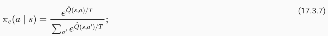
whereεis called the “exploration parameter” and is chosen by the user. The policy πeis called an exploration policy. This particular πeis called anε-greedy exploration policy because it chooses the optimal action (under the current estimateQ^) with probability1−εbut explores randomly with the remainder probabilityε. We can also use the so-called softmax exploration policy
여기서 ε는 "탐색 매개변수"라고 하며 사용자가 선택합니다. 정책 πe를 탐사 정책이라고 합니다. 이 특정 πe는 확률 1−ε로 최적의 행동(현재 추정치 Q^ 하에서)을 선택하지만 나머지 확률 ε으로 무작위로 탐색하기 때문에 ε-탐욕 탐색 정책이라고 합니다. 소위 소프트맥스 탐색 정책을 사용할 수도 있습니다.
where the hyper-parameterTis called temperature. A large value ofεinε-greedy policy functions similarly to a large value of temperatureTfor the softmax policy.
여기서 초매개변수 T를 온도라고 합니다. ε-탐욕 정책에서 ε의 큰 값은 소프트맥스 정책의 온도 T의 큰 값과 유사하게 기능합니다.
It is important to note that when we pick an exploration that depends upon the current estimate of the action-value functionQ^, we need to resolve the optimization problem periodically. Typical implementations of Q-Learning make one mini-batch update using a few state-action pairs in the collected dataset (typically the ones collected from the previous timestep of the robot) after taking every action using πe.
행동-가치 함수 Q^의 현재 추정에 의존하는 탐색을 선택할 때 최적화 문제를 주기적으로 해결해야 한다는 점에 유의하는 것이 중요합니다. Q-Learning의 일반적인 구현은 πe를 사용하여 모든 작업을 수행한 후 수집된 데이터 세트(일반적으로 로봇의 이전 단계에서 수집된 데이터)의 몇 가지 상태-작업 쌍을 사용하여 하나의 미니 배치 업데이트를 수행합니다.
17.3.4.The “Self-correcting” Property of Q-Learning
The dataset collected by the robot during Q-Learning grows with time. Both the exploration policy πeand the estimateQ^evolve as the robot collects more data. This gives us a key insight into why Q-Learning works well. Consider a states: if a particular actionahas a large value under the current estimateQ^(s,a), then both the ε-greedy and the softmax exploration policies have a larger probability of picking this action. If this action actually isnotthe ideal action, then the future states that arise from this action will have poor rewards. The next update of the Q-Learning objective will therefore reduce the valueQ^(s,a), which will reduce the probability of picking this action the next time the robot visits states. Bad actions, e.g., ones whose value is overestimated inQ^(s,a), are explored by the robot but their value is correct in the next update of the Q-Learning objective. Good actions, e.g., whose valueQ^(s,a)is large, are explored more often by the robot and thereby reinforced. This property can be used to show that Q-Learning can converge to the optimal policy even if it begins with a random policy πe(Watkins and Dayan, 1992).
Q-Learning 중에 로봇이 수집한 데이터 세트는 시간이 지남에 따라 증가합니다. 탐색 정책 πe와 추정치 Q^는 모두 로봇이 더 많은 데이터를 수집함에 따라 진화합니다. 이는 Q-Learning이 왜 잘 작동하는지에 대한 중요한 통찰력을 제공합니다. 상태 s를 고려하십시오. 특정 작업 a가 현재 추정치 Q^(s,a)보다 큰 값을 갖는 경우 ε-탐욕 및 소프트맥스 탐색 정책 모두 이 작업을 선택할 확률이 더 높습니다. 만약 이 행동이 실제로 이상적인 행동이 아니라면, 이 행동에서 발생하는 미래 상태는 낮은 보상을 받게 될 것입니다. 따라서 Q-Learning 목표의 다음 업데이트는 Q^(s,a) 값을 줄여 로봇이 다음에 상태 s를 방문할 때 이 작업을 선택할 확률을 줄입니다. 나쁜 행동, 예를 들어 Q^(s,a)에서 값이 과대평가된 행동은 로봇에 의해 탐색되지만 그 값은 Q-Learning 목표의 다음 업데이트에서 정확합니다. 예를 들어 Q^(s,a) 값이 큰 좋은 행동은 로봇에 의해 더 자주 탐색되어 강화됩니다. 이 속성은 Q-Learning이 무작위 정책 πe로 시작하더라도 최적의 정책으로 수렴할 수 있음을 보여주는 데 사용될 수 있습니다(Watkins and Dayan, 1992).
This ability to not only collect new data but also collect the right kind of data is the central feature of reinforcement learning algorithms, and this is what distinguishes them from supervised learning. Q-Learning, using deep neural networks (which we will see in the DQN chapeter later), is responsible for the resurgence of reinforcement learning(Mnihet al., 2013).
새로운 데이터를 수집할 뿐만 아니라 올바른 종류의 데이터를 수집하는 이러한 능력은 강화 학습 알고리즘의 핵심 기능이며 지도 학습과 구별됩니다. 심층 신경망(나중에 DQN 장에서 볼 예정)을 사용하는 Q-Learning은 강화 학습의 부활을 담당합니다(Mnih et al., 2013).
17.3.5.Implementation of Q-Learning
We now show how to implement Q-Learning on FrozenLake fromOpen AI Gym. Note this is the same setup as we consider inValue Iterationexperiment.
이제 Open AI Gym의 FrozenLake에서 Q-Learning을 구현하는 방법을 보여줍니다. 이는 Value Iteration 실험에서 고려한 것과 동일한 설정입니다.
%matplotlib inline
import random
import numpy as np
from d2l import torch as d2l

seed = 0  # Random number generator seed
gamma = 0.95  # Discount factor
num_iters = 256  # Number of iterations
alpha   = 0.9  # Learing rate
epsilon = 0.9  # Epsilon in epsilion gready algorithm
random.seed(seed)  # Set the random seed
np.random.seed(seed)

# Now set up the environment
env_info = d2l.make_env('FrozenLake-v1', seed=seed)
이 코드는 강화 학습 문제를 해결하기 위한 환경 설정을 합니다. 구체적으로는 FrozenLake-v1 환경에서 Q-Learning 알고리즘을 실행하기 위한 환경을 설정하는 부분입니다. 코드의 주요 요소를 설명하겠습니다.
%matplotlib inline: 이 라인은 주피터 노트북(Jupyter Notebook)에서 그래프 및 플롯을 인라인으로 표시하도록 지시합니다.
import random: 파이썬의 random 모듈을 가져옵니다. 이 모듈은 난수 생성과 관련된 함수를 제공합니다.
import numpy as np: NumPy 라이브러리를 가져옵니다. NumPy는 과학적 계산을 위한 파이썬 라이브러리로, 다차원 배열과 관련된 기능을 제공합니다. 주로 행렬 연산과 숫자 계산에 사용됩니다.
from d2l import torch as d2l: "d2l" 패키지에서 "torch" 모듈을 가져와서 "d2l"로 별명을 붙입니다. 이 패키지는 "Dive into Deep Learning" 책의 코드와 유틸리티 함수를 제공합니다.
seed = 0: 랜덤 시드(seed)를 0으로 설정합니다. 시드를 설정하면 랜덤 함수 호출 결과가 항상 동일하게 유지됩니다. 이렇게 하면 실험의 재현성을 확보할 수 있습니다.
gamma = 0.95: 감쇠 요인(gamma)을 설정합니다. 감쇠 요인은 미래 보상의 가치를 현재 보상의 가치보다 얼마나 가중치를 둘 것인지 결정하는 요소입니다.
num_iters = 256: Q-Learning의 반복 횟수를 설정합니다. 즉, 학습을 몇 번 반복할 것인지를 결정합니다.
alpha = 0.9: 학습률(learning rate)을 설정합니다. 학습률은 Q-Value를 업데이트할 때 현재 값과 새로운 값을 얼마나 가중치를 두고 합칠지를 결정하는 요소입니다.
epsilon = 0.9: 엡실론(epsilon) 값을 설정합니다. 엡실론은 엡실론-그리디(epsilon-greedy) 알고리즘에서 사용되며, 탐험(Exploration)과 이용(Exploitation) 사이의 균형을 조절하는 역할을 합니다.
random.seed(seed), np.random.seed(seed): 랜덤 시드를 설정하여 실험 결과의 재현성을 확보합니다. 같은 시드를 사용하면 같은 조건에서 항상 같은 결과를 얻을 수 있습니다.
env_info = d2l.make_env('FrozenLake-v1', seed=seed): 'FrozenLake-v1'이라는 환경을 생성하고, 시드(seed)를 설정합니다. FrozenLake-v1은 강화 학습을 위한 환경으로, 얼어붙은 호수에서 목표 지점까지 에이전트를 이동시키는 과제를 제공합니다.
이제 이 설정된 환경에서 Q-Learning 알고리즘을 실행할 수 있습니다.
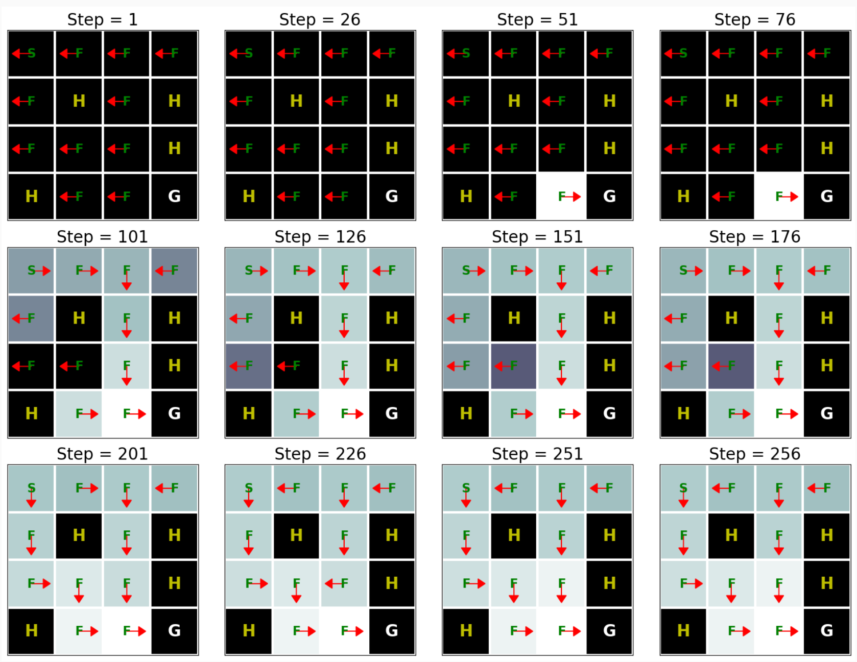
In the FrozenLake environment, the robot moves on a4×4grid (these are the states) with actions that are “up” (↑), “down” (→), “left” (←), and “right” (→). The environment contains a number of holes (H) cells and frozen (F) cells as well as a goal cell (G), all of which are unknown to the robot. To keep the problem simple, we assume the robot has reliable actions, i.e. P(s′∣s,a)=1for all s∈S,a∈A. If the robot reaches the goal, the trial ends and the robot receives a reward of1irrespective of the action; the reward at any other state is0for all actions. The objective of the robot is to learn a policy that reaches the goal location (G) from a given start location (S) (this is s0) to maximize thereturn.
FrozenLake 환경에서 로봇은 "위"(↑), "아래"(→), "왼쪽"(←), "오른쪽"( →). 환경에는 다수의 구멍(H) 세포와 동결(F) 세포 및 목표 세포(G)가 포함되어 있으며, 이들 모두는 로봇에 알려지지 않습니다. 문제를 단순하게 유지하기 위해 로봇이 신뢰할 수 있는 동작을 한다고 가정합니다. 즉, 모든 s∈S,a∈A에 대해 P(s′∣s,a)=1입니다. 로봇이 목표에 도달하면 시험이 종료되고 로봇은 행동에 관계없이 1의 보상을 받습니다. 다른 상태에서의 보상은 모든 행동에 대해 0입니다. 로봇의 목적은 주어진 시작 위치(S)(이것은 s0)에서 목표 위치(G)에 도달하는 정책을 학습하여 수익을 극대화하는 것입니다.
We first implementε-greedy method as follows:
def e_greedy(env, Q, s, epsilon):
    if random.random() < epsilon:
        return env.action_space.sample()

    else:
        return np.argmax(Q[s,:])
이 코드는 엡실론-그리디(epsilon-greedy) 알고리즘을 구현한 함수입니다. 이 알고리즘은 강화 학습에서 탐험(Exploration)과 이용(Exploitation) 사이의 균형을 조절하기 위해 사용됩니다. 엡실론-그리디 알고리즘은 주어진 상황에서 랜덤한 행동을 선택할 확률과 현재 학습한 최적 행동을 선택할 확률을 조절합니다.
여기서 각 인자의 의미를 설명하겠습니다:
env: 강화 학습 환경입니다. 이 환경에서 에이전트는 행동을 선택하고 보상을 받습니다.
Q: Q-Value 함수로, 각 상태(state) 및 행동(action)에 대한 가치를 나타내는 배열입니다. Q[s, a]는 상태 s에서 행동 a를 선택했을 때의 가치를 나타냅니다.
s: 현재 상태를 나타내는 변수입니다.
epsilon: 엡실론(epsilon) 값으로, [0, 1] 범위의 확률값입니다. 엡실론은 랜덤한 행동을 선택할 확률을 결정하는 매개변수입니다.
이 함수의 동작은 다음과 같습니다:
random.random() < epsilon: 랜덤한 확률값을 생성하고 이 값이 엡실론 값보다 작은지를 확인합니다. 엡실론 값보다 작으면 랜덤한 행동을 선택하게 됩니다. 이것은 탐험(Exploration)을 의미합니다. 즉, 에이전트는 새로운 경험을 얻기 위해 무작위로 행동을 선택합니다.
엡실론 값보다 크면, Q-Value 함수를 통해 현재 상태 s에서 가능한 행동 중에서 가치가 가장 높은 행동을 선택합니다. 이것은 이용(Exploitation)을 의미합니다. 에이전트는 학습한 지식을 활용하여 최적의 행동을 선택합니다.
따라서 이 함수는 엡실론 확률에 따라 탐험과 이용을 조절하여 행동을 선택합니다.
We are now ready to implement Q-learning:
이제 Q-learning을 구현할 준비가 되었습니다.
def q_learning(env_info, gamma, num_iters, alpha, epsilon):
    env_desc = env_info['desc']  # 2D array specifying what each grid item means
    env = env_info['env']  # 2D array specifying what each grid item means
    num_states = env_info['num_states']
    num_actions = env_info['num_actions']

    Q  = np.zeros((num_states, num_actions))
    V  = np.zeros((num_iters + 1, num_states))
    pi = np.zeros((num_iters + 1, num_states))

    for k in range(1, num_iters + 1):
        # Reset environment
        state, done = env.reset(), False
        while not done:
            # Select an action for a given state and acts in env based on selected action
            action = e_greedy(env, Q, state, epsilon)
            next_state, reward, done, _ = env.step(action)

            # Q-update:
            y = reward + gamma * np.max(Q[next_state,:])
            Q[state, action] = Q[state, action] + alpha * (y - Q[state, action])

            # Move to the next state
            state = next_state
        # Record max value and max action for visualization purpose only
        for s in range(num_states):
            V[k,s]  = np.max(Q[s,:])
            pi[k,s] = np.argmax(Q[s,:])
    d2l.show_Q_function_progress(env_desc, V[:-1], pi[:-1])

q_learning(env_info=env_info, gamma=gamma, num_iters=num_iters, alpha=alpha, epsilon=epsilon)
이 코드는 Q-Learning 알고리즘을 구현하여 강화 학습을 수행하는 함수입니다. Q-Learning은 강화 학습에서 가치 반복(Value Iteration)을 기반으로 하는 모델-프리(Model-Free) 강화 학습 알고리즘 중 하나로, 에이전트가 최적의 행동을 학습하는 방법 중 하나입니다.
여기서 각 인자의 의미를 설명하겠습니다:
env_info: 강화 학습 환경 정보입니다. 환경의 구조와 관련된 정보가 포함되어 있습니다.
gamma: 감쇠 계수(Discount Factor)로서 미래 보상의 현재 가치에 대한 중요성을 조절하는 매개변수입니다.
num_iters: 반복 횟수로서 학습을 몇 번 반복할지 결정하는 매개변수입니다.
alpha: 학습률(learning rate)로서 Q-Value를 업데이트할 때 얼마나 큰 보정을 적용할지 결정하는 매개변수입니다.
초기 Q-Value 함수(Q)와 가치 함수(V)를 0으로 초기화합니다. 또한 정책 함수(pi)를 0으로 초기화합니다.
주어진 반복 횟수(num_iters)만큼 아래의 과정을 반복합니다:
환경을 초기화하고 시작 상태(state)를 얻습니다.
에이전트는 엡실론-그리디 알고리즘을 사용하여 현재 상태(state)에서 행동(action)을 선택합니다. 엡실론 확률에 따라 랜덤한 탐험 행동 또는 학습한 Q-Value를 기반으로 한 최적 행동을 선택합니다.
선택한 행동을 환경에 적용하고 다음 상태(next_state), 보상(reward), 종료 여부(done) 등을 얻습니다.
Q-Value 업데이트를 수행합니다. Q-Learning의 핵심은 Q-Value 업데이트 공식인 Bellman Equation을 사용하여 Q-Value를 업데이트하는 것입니다. 새로운 가치(y)는 현재 보상(reward)과 다음 상태의 최대 Q-Value(gamma * np.max(Q[next_state,:]))를 합친 값으로 계산됩니다. 그리고 이 값을 사용하여 Q-Value를 업데이트합니다.
다음 상태로 이동합니다.
각 반복에서 가치 함수(V)와 정책 함수(pi)를 업데이트하고 시각화를 위해 저장합니다.
이렇게 반복적으로 Q-Value를 업데이트하고 최적의 정책을 학습하여 환경에서 에이전트가 최적의 행동을 선택할 수 있도록 합니다.
This result shows that Q-learning can find the optimal solution for this problem roughly after 250 iterations. However, when we compare this result with the Value Iteration algorithm’s result (seeImplementation of Value Iteration), we can see that the Value Iteration algorithm needs way fewer iterations to find the optimal solution for this problem. This happens because the Value Iteration algorithm has access to the full MDP whereas Q-learning does not.
이 결과는 Q-learning이 대략 250번의 반복 후에 이 문제에 대한 최적의 솔루션을 찾을 수 있음을 보여줍니다. 그러나 이 결과를 Value Iteration 알고리즘의 결과(Value Iteration 구현 참조)와 비교하면 Value Iteration 알고리즘이 이 문제에 대한 최적의 솔루션을 찾기 위해 훨씬 더 적은 반복이 필요하다는 것을 알 수 있습니다. 이는 Value Iteration 알고리즘이 전체 MDP에 액세스할 수 있는 반면 Q-learning은 액세스할 수 없기 때문에 발생합니다.
17.3.6.Summary
Q-learning is one of the most fundamental reinforcement-learning algorithms. It has been at the epicenter of the recent success of reinforcement learning, most notably in learning to play video games(Mnihet al., 2013). Implementing Q-learning does not require that we know the Markov decision process (MDP), e.g., the transition and reward functions, completely.
Q-러닝은 가장 기본적인 강화학습 알고리즘 중 하나입니다. 이는 최근 강화 학습 성공의 진원지였으며, 특히 비디오 게임 학습에서 가장 두드러졌습니다(Mnih et al., 2013). Q-러닝을 구현하기 위해 MDP(Markov Decision Process)(예: 전환 및 보상 기능)를 완전히 알 필요는 없습니다.
In this section we will discuss how to pick the best action for the robot at each state to maximize thereturnof the trajectory. We will describe an algorithm called Value Iteration and implement it for a simulated robot that travels over a frozen lake.
이 섹션에서는 Return of the trajectory (궤적 반환)을 최대화하기 위해 각 state에서 robot에 대한 최상의 action을 선택하는 방법을 설명할 것입니다. Value Iteration이라는 알고리즘을 설명하고 이를 얼어붙은 호수 위를 이동하는 시뮬레이션 로봇에 대해 구현해 보겠습니다.
Value Iteration이란?
'Value Iteration(가치 반복)'은 강화 학습(Reinforcement Learning)에서 사용되는 동적 프로그래밍(Dynamic Programming) 알고리즘 중 하나입니다. 가치 반복은 마르코프 결정 과정(Markov Decision Process, MDP)에서 최적 가치 함수(optimal value function)를 근사화하기 위해 사용됩니다.
MDP에서 가치 함수(value function)는 각 상태(state)의 가치를 측정하며, 최적 가치 함수는 최상의 정책(policy)을 찾기 위한 중요한 개념입니다. 가치 반복은 다음 단계로 진행됩니다:
Initialization(초기화): 가치 함수를 초기화합니다. 보통 모든 상태의 가치를 0으로 초기화하거나 임의의 값으로 초기화합니다.
Iterative Update(반복 업데이트): 반복적으로 현재의 가치 함수를 업데이트합니다. 이 업데이트는 다음과 같은 벨만 최적 방정식(Bellman Optimality Equation)을 사용하여 이루어집니다.
상태 가치 업데이트(State Value Update): 모든 상태에 대해 현재 상태의 가치를 주변 상태의 가치와 보상을 고려하여 업데이트합니다. 이때 가치 함수는 최대값을 가지는 방향으로 업데이트됩니다.
행동 가치 업데이트(Action Value Update): 상태 대신 상태-행동 쌍(state-action pair)에 대한 가치 함수를 업데이트합니다. 이는 에이전트가 각 상태에서 가능한 모든 행동에 대한 가치를 나타냅니다.
Convergence(수렴): 가치 함수가 수렴할 때까지 반복 업데이트를 수행합니다. 일반적으로 두 가지 가치 함수 간의 차이가 어떤 임계값 이하로 작아질 때 알고리즘을 종료합니다.
Policy Extraction(정책 추출): 최적 가치 함수를 기반으로 최적 정책을 추출합니다. 이 최적 정책은 에이전트가 각 상태에서 어떤 행동을 선택해야 하는지를 나타냅니다.
가치 반복은 최적 정책과 최적 가치 함수를 찾는 강화 학습 문제에서 효과적으로 사용됩니다. 하지만 모든 가능한 상태-행동 쌍에 대해 가치 함수를 업데이트하므로 상태와 행동의 공간이 크면 계산 비용이 높을 수 있습니다.
Return of the trajectory 란?
In the context of hyperparameter optimization or any optimization process, the "trajectory" typically refers to the path or sequence of points that the optimizer explores during the search for the optimal solution. Each point on this trajectory corresponds to a specific configuration of hyperparameters, and the trajectory represents how the objective function (or some other evaluation metric) changes as the optimizer moves from one configuration to another.
하이퍼파라미터 최적화 또는 다른 최적화 과정에서 "궤적(trajectory)"은 일반적으로 옵티마이저가 최적해를 찾기 위해 탐색하는 지점 또는 순서를 나타냅니다. 이 궤적 상의 각 지점은 하이퍼파라미터의 특정 설정에 해당하며, 궤적은 옵티마이저가 한 설정에서 다른 설정으로 이동함에 따라 목적 함수(또는 다른 평가 지표)가 어떻게 변화하는지를 나타냅니다.
The "return of the trajectory" usually refers to the value of the objective function at the final point or configuration reached by the optimizer after its search process is complete. In the context of hyperparameter optimization, this would be the performance or error metric associated with the best set of hyperparameters found by the optimizer.
"궤적의 반환(return of the trajectory)"은 보통 최적화 과정이 완료된 후 옵티마이저가 도달한 최종 지점 또는 설정에서의 목적 함수 값을 나타냅니다. 하이퍼파라미터 최적화의 맥락에서 이것은 최적화 과정을 통해 찾은 하이퍼파라미터 집합으로 모델을 훈련할 때 얻는 성능 또는 에러 지표와 관련됩니다.
For example, if you're using a hyperparameter tuning algorithm to find the best hyperparameters for a machine learning model, the "return of the trajectory" would represent the final performance (e.g., accuracy, loss, etc.) achieved by the model when trained with the hyperparameters discovered by the optimization process.
예를 들어, 기계 학습 모델의 최적 하이퍼파라미터를 찾기 위해 하이퍼파라미터 튜닝 알고리즘을 사용 중이라면 "궤적의 반환"은 최적화 과정 중 발견된 하이퍼파라미터 집합으로 훈련된 모델의 최종 성능(정확도, 손실 등)을 나타낼 것입니다.
In summary, "return of the trajectory" is a way to describe the outcome or result of the optimization process, which is often measured by the performance achieved with the best set of hyperparameters found during the search.
요약하면, "궤적의 반환"은 최적화 과정의 결과 또는 최적화 과정 중 찾은 최상의 하이퍼파라미터 설정을 사용했을 때 얻는 성능으로, 최적화 과정의 결과물을 나타내는 방식입니다.
17.2.1.Stochastic Policy 확률적 정책
A stochastic policy denoted asπ(a∣s)(policy for short) is a conditional distribution over the actionsa∈Agiven the states∈S,π(a∣s)≡P(a∣s). As an example, if the robot has four actionsA={go left, go down, go right, go up}. The policy at a states∈Sfor such a set of actionsAis a categorical distribution where the probabilities of the four actions could be[0.4,0.2,0.1,0.3]; at some other states′∈Sthe probabilitiesπ(a∣s′)of the same four actions could be[0.1,0.1,0.2,0.6]. Note that we should have∑a π(a∣s)=1for any states. A deterministic policy is a special case of a stochastic policy in that the distributionπ(a∣s)only gives non-zero probability to one particular action, e.g.,[1,0,0,0]for our example with four actions.
π(a∣s)(간단히 정책)로 표시되는 확률론적 정책은 상태 s∈S, π(a∣s)=P(a∣s)가 주어지면 동작 a∈A에 대한 조건부 분포입니다. 예를 들어, 로봇에 4가지 동작 A= {왼쪽으로 이동, 아래로 이동, 오른쪽으로 이동, 위로 이동}이 있는 경우입니다. 그러한 일련의 행동 A에 대한 상태 s∈S의 정책은 네 가지 행동의 확률이 [0.4,0.2,0.1,0.3]이 될 수 있는 범주형 분포입니다. 다른 상태 s′∈S에서 동일한 네 가지 행동의 확률 π(a∣s′)는 [0.1,0.1,0.2,0.6]이 될 수 있습니다. 모든 상태 s에 대해 ∑a π(a∣s)=1이 있어야 합니다. 결정론적 정책은 분포 π(a∣s)가 하나의 특정 작업에만 0이 아닌 확률을 제공한다는 점에서 확률론적 정책의 특별한 경우입니다(예: 4개 작업이 있는 예시의 경우 [1,0,0,0]).
Stochastic Policy란?
In the context of reinforcement learning, a "stochastic policy" refers to a strategy or a set of rules that an agent uses to make decisions in an environment. What makes it "stochastic" is that it introduces an element of randomness or probability into the decision-making process.
Reinforcement learning(강화 학습)의 맥락에서 '확률적 정책'은 에이전트가 환경에서 의사 결정을 내리는 데 사용하는 전략이나 규칙을 가리킵니다. 이것이 '확률적'으로 만드는 것은 의사 결정 프로세스에 확률 또는 무작위성 요소를 도입한다는 것입니다.
In a stochastic policy, the agent doesn't make deterministic choices, where every action is known in advance. Instead, it selects actions based on a probability distribution. This means that even in the same state, the agent might choose different actions in different episodes or trials, reflecting the inherent uncertainty in the environment or the agent's own decision-making process.
확률적 정책에서 에이전트는 결정을 내릴 때 미리 모든 행동이 알려져 있는 결정적 선택을 하지 않습니다. 대신, 확률 분포를 기반으로 행동을 선택합니다. 이것은 동일한 상태에서라도 에이전트가 다른 에피소드나 시도에서 다른 행동을 선택할 수 있음을 의미하며, 이는 환경의 불확실성이나 에이전트 자체의 의사 결정 프로세스에 내재된 불확실성을 반영합니다.
Stochastic policies are often represented as probability distributions over possible actions. The agent samples from this distribution to select an action. The degree of randomness or variability in the policy can vary depending on the specific problem and learning algorithm. Stochastic policies can be advantageous in situations where variability in actions is desirable to explore the environment more effectively or handle uncertainties.
확률적 정책은 종종 가능한 행동에 대한 확률 분포로 표현됩니다. 에이전트는 이 분포에서 샘플링하여 행동을 선택합니다. 정책의 무작위성이나 변동성의 정도는 구체적인 문제 및 학습 알고리즘에 따라 다를 수 있습니다. 환경을 더 효과적으로 탐색하거나 불확실성을 다루기 위해 행동의 변동성이 바람직한 상황에서 확률적 정책을 사용하는 것이 유리할 수 있습니다.
In contrast, a "deterministic policy" would map each state directly to a specific action without any randomness, meaning that in the same state, the agent would always choose the same action.
반면, '결정적 정책'은 각 상태를 특정한 행동에 직접 매핑하며 어떠한 무작위성도 없이 특정한 행동을 선택한다는 것을 의미합니다.
Stochastic policies are commonly used in reinforcement learning algorithms, such as policy gradient methods, to enable exploration and adaptability in dynamic environments.
확률적 정책은 주로 정책 그래디언트 방법 등의 강화 학습 알고리즘에서 사용되며, 동적 환경에서의 탐색과 적응을 가능하게 하기 위해 활용됩니다.
17.2.2.Value Function
Imagine now that the robot starts at a states0and at each time instant, it first samples an action from the policyat∼π(st)and takes this action to result in the next statest+1. The trajectoryτ=(s0,a0,r0,s1,a1,r1,…), can be different depending upon which particular actionatis sampled at intermediate instants. We define the averagereturnR(τ)=∑**∞ t=0 γ**t r(st,at)of all such trajectories
이제 로봇이 상태 s0에서 시작하고 매 순간마다 먼저 ∼π(st)의 정책에서 작업을 샘플링하고 이 작업을 수행하여 다음 상태 st+1을 생성한다고 상상해 보세요. 궤적 τ=(s0,a0,r0,s1,a1,r1,…)은 중간 순간에 샘플링되는 특정 동작에 따라 다를 수 있습니다. 우리는 그러한 모든 궤적의 평균 수익률 R(τ)=∑**킵 t=0 γ**t r(st,at)을 정의합니다.
wheres t+1∼P(st+1∣st,at)is the next state of the robot andr(st,at)is the instantaneous reward obtained by taking action 'at'in statestat timet. This is called the “value function” for the policyπ. In simple words, the value of a states0for a policyπ, denoted byV**π(s0), is the expectedϒ-discountedreturnobtained by the robot if it begins at states0and takes actions from the policyπat each time instant.
여기서 s t+1∼P(st+1∣st,at)는 로봇의 다음 상태이고, r(st,at)는 시간 t에서 상태 st에서 'at' 행동을 취함으로써 얻은 순간 보상이다. 이를 정책 π에 대한 "가치 함수"라고 합니다. 간단히 말해서, V**π(s0)로 표시되는 정책 π에 대한 상태 s0의 값은 기대되는 ϒ-할인된 수익입니다. 이것은 로봇이 상태 s0에서 시작하고 매 순간마다 정책 π에서 조치를 취하는 경우 로봇에 의해 수행되는 것에 의해 얻어집니다.
We next break down the trajectory into two stages (i) the first stage which corresponds tos0→s1upon taking the actiona0, and (ii) a second stage which is the trajectoryτ′=(s1,a1,r1,…)thereafter. The key idea behind all algorithms in reinforcement learning is that the value of states0can be written as the average reward obtained in the first stage and the value function averaged over all possible next statess1. This is quite intuitive and arises from our Markov assumption: the average return from the current state is the sum of the average return from the next state and the average reward of going to the next state. Mathematically, we write the two stages as
다음으로 궤도를 두 단계로 나눕니다. (i) 조치 a0을 취했을 때 s0→s1에 해당하는 첫 번째 단계, (ii) 궤도 τ'=(s1,a1,r1,…)인 두 번째 단계 - 이러한 상황이 계속 이어짐 . 강화 학습의 모든 알고리즘 뒤에 있는 핵심 아이디어는 상태 s0의 값이 첫 번째 단계에서 얻은 평균 보상으로 기록될 수 있고 가치 함수가 가능한 모든 다음 상태 s1에 대해 평균을 낼 수 있다는 것입니다. 이는 매우 직관적이며 Markov 가정에서 비롯됩니다. 현재 상태의 평균 수익은 다음 상태의 평균 수익과 다음 상태로 이동하는 평균 보상의 합입니다. 수학적으로 우리는 두 단계를 다음과 같이 씁니다.
This decomposition is very powerful: it is the foundation of the principle of dynamic programming upon which all reinforcement learning algorithms are based. Notice that the second stage gets two expectations, one over the choices of the actiona0taken in the first stage using the stochastic policy and another over the possible statess1obtained from the chosen action. We can write(17.2.2)using the transition probabilities in the Markov decision process (MDP) as
이러한 분해는 매우 강력합니다. 이는 모든 강화 학습 알고리즘의 기반이 되는 동적 프로그래밍 원리의 기초입니다. 두 번째 단계에서는 확률론적 정책을 사용하여 첫 번째 단계에서 취한 행동 a0의 선택에 대한 기대와 선택한 행동에서 얻은 가능한 상태 s1에 대한 기대라는 두 가지 기대를 얻습니다. 마르코프 결정 과정(MDP)의 전환 확률을 사용하여 (17.2.2)를 다음과 같이 작성할 수 있습니다.
An important thing to notice here is that the above identity holds for all statess∈Sbecause we can think of any trajectory that begins at that state and break down the trajectory into two stages.
여기서 주목해야 할 중요한 점은 위의 항등식이 모든 상태 s∈S에 대해 적용된다는 것입니다. 왜냐하면 우리는 해당 상태에서 시작하는 모든 궤적을 생각하고 궤적을 두 단계로 나눌 수 있기 때문입니다.
Value Function이란?
In the context of reinforcement learning, a "value function" is a fundamental concept used to estimate the expected cumulative rewards an agent can obtain when following a particular policy in an environment. Value functions are essential for making decisions and learning in reinforcement learning tasks.
강화 학습의 맥락에서 '가치 함수(Value Function)'는 특정 환경에서 특정 정책을 따를 때 에이전트가 기대하는 누적 보상을 추정하는 데 사용되는 기본 개념입니다. 가치 함수는 강화 학습 작업에서의 의사 결정 및 학습에 필수적입니다.
There are two main types of value functions:
주로 두 가지 유형의 가치 함수가 있습니다:
State-Value Function (V(s)): This function estimates the expected cumulative reward an agent can achieve when starting from a particular state and following a specific policy. In other words, V(s) quantifies the long-term desirability of being in a given state while following the chosen policy.
상태 가치 함수 (V(s)): 이 함수는 특정 상태에서 시작하여 특정 정책을 따를 때 에이전트가 기대하는 누적 보상을 추정합니다. 다시 말해, V(s)는 선택한 정책을 따를 때 주어진 상태에 있을 때의 장기적인 바람직함을 측정합니다.
Action-Value Function (Q(s, a)): This function estimates the expected cumulative reward an agent can obtain by taking a particular action (a) in a specific state (s) and then following a specific policy. Q(s, a) measures the long-term desirability of taking a particular action in a given state while following the chosen policy.
행동 가치 함수 (Q(s, a)): 이 함수는 특정 상태 (s)에서 특정 행동 (a)을 취한 다음 특정 정책을 따를 때 에이전트가 기대하는 누적 보상을 추정합니다. Q(s, a)는 주어진 상태에서 특정 행동을 취할 때 선택한 정책을 따를 때의 장기적인 바람직함을 측정합니다.
Value functions are crucial for various reinforcement learning algorithms, such as Q-learning and policy gradient methods. They serve as a foundation for evaluating and comparing different policies. By iteratively updating these value functions, an agent can learn to make better decisions and maximize its cumulative rewards in the environment.
가치 함수는 Q-러닝(Q-learning) 및 정책 그래디언트 방법과 같은 다양한 강화 학습 알고리즘에서 중요합니다. 이들은 서로 다른 정책을 평가하고 비교하는 데 기초를 제공합니다. 이러한 가치 함수를 반복적으로 업데이트함으로써 에이전트는 더 나은 결정을 내리고 환경에서 누적 보상을 최대화하는 방법을 학습할 수 있습니다.
The ultimate goal of reinforcement learning is often to find an optimal policy, which is a policy that maximizes the expected cumulative reward. Value functions are essential tools for achieving this goal because they help assess and improve policies based on their expected performance.
강화 학습의 궁극적인 목표는 종종 기대 누적 보상을 최대화하는 최적 정책을 찾는 것입니다. 가치 함수는 이 목표를 달성하기 위한 중요한 도구입니다.
17.2.3.Action-Value Function
In implementations, it is often useful to maintain a quantity called the “action value” function which is a closely related quantity to the value function. This is defined to be the averagereturnof a trajectory that begins ats0but when the action of the first stage is fixed to be
구현에서는 가치 함수와 밀접하게 관련된 수량인 "액션 가치" 함수라는 수량을 유지하는 것이 유용한 경우가 많습니다. 이는 s0에서 시작하지만 첫 번째 단계의 동작이 다음과 같이 고정된 궤적의 평균 반환으로 정의됩니다.
note that the summation inside the expectation is fromt=1,…,∞because the reward of the first stage is fixed in this case. We can again break down the trajectory into two parts and write
이 경우 첫 번째 단계의 보상이 고정되어 있기 때문에 기대값 내부의 합은 t=1,...,부터라는 점에 유의하세요. 우리는 다시 궤적을 두 부분으로 나누고 다음과 같이 쓸 수 있습니다.
This version is the analog of(17.2.3)for the action value function.
이 버전은 동작 값 함수에 대한 (17.2.3)과 유사합니다.
Action Value Function이란?
In the context of reinforcement learning, the "Action-Value Function," often denoted as Q(s, a), represents the expected cumulative reward an agent can obtain by taking a specific action (a) in a particular state (s) and then following a specific policy. It quantifies the long-term desirability of taking a particular action in a given state while adhering to the chosen policy.
강화 학습의 맥락에서 '행동 가치 함수(Action-Value Function)'는 특정 상태 (s)에서 특정 행동 (a)을 취한 다음 특정 정책을 따를 때 에이전트가 기대하는 누적 보상을 나타냅니다. 이는 선택한 정책을 따를 때 주어진 상태에서 특정 행동을 취하는 것의 장기적인 바람직함을 측정합니다.
Here's a breakdown of the components of the Action-Value Function (Q(s, a)):
행동 가치 함수 (Q(s, a))의 구성 요소를 살펴보겠습니다:
s (state): This is the current situation or configuration of the environment that the agent perceives.
s (상태): 이것은 에이전트가 지각하는 환경의 현재 상황 또는 구성입니다.
a (action): This is the specific action that the agent takes in the current state.
a (행동): 이것은 에이전트가 현재 상태에서 취하는 구체적인 행동입니다.
Q(s, a): This is the Action-Value Function, which provides an estimate of the expected cumulative reward starting from state s, taking action a, and then following a specific policy.
Q(s, a): 이것은 행동 가치 함수로, 상태 s에서 행동 a를 취하고 특정 정책을 따를 때 기대하는 누적 보상을 추정합니다.
The Action-Value Function is fundamental in reinforcement learning because it helps the agent evaluate and compare different actions in a given state. By computing the Q-values for each action in each state and following a specific policy, an agent can make informed decisions to maximize its cumulative rewards over time.
행동 가치 함수는 강화 학습에서 기본적이며, 에이전트가 주어진 상태에서 다른 행동을 평가하고 비교하는 데 도움을 줍니다. 각 상태에서 각 행동의 Q-값을 계산하고 특정 정책을 따를 때, 에이전트는 시간이 지남에 따라 누적 보상을 최대화하기 위한 정보에 기반하여 결정을 내릴 수 있습니다.
One of the key algorithms that uses the Action-Value Function is Q-learning, which aims to learn the optimal action-value function (Q-function) that maximizes the expected cumulative reward. This function is often used to guide the agent's behavior in an environment, allowing it to learn to make better decisions over time.
행동 가치 함수를 사용하는 주요 알고리즘 중 하나는 Q-러닝(Q-learning)입니다. 이 알고리즘은 기대 누적 보상을 최대화하는 행동 가치 함수 (Q-함수)를 학습하는 것을 목표로 하며, 이 함수는 환경에서 에이전트의 행동을 안내하는 데 자주 사용됩니다. 에이전트는 시간이 지남에 따라 더 나은 결정을 내리도록 학습하게 됩니다.
17.2.4.Optimal Stochastic Policy
Both the value function and the action-value function depend upon the policy that the robot chooses. We will next think of the “optimal policy” that achieves the maximal averagereturn
가치 함수와 행동-가치 함수는 모두 로봇이 선택하는 정책에 따라 달라집니다. 다음으로 최대 평균수익률을 달성하는 '최적정책'에 대해 생각해 보겠습니다.
Of all possible stochastic policies that the robot could have taken, the optimal policyπ*achieves the largest average discountedreturnfor trajectories starting from states0. Let us denote the value function and the action-value function of the optimal policy asV*≡Vπ*andQ*≡Qπ*.
로봇이 취할 수 있는 모든 가능한 확률론적 정책 중에서 최적 정책 π*는 상태 s0에서 시작하는 궤도에 대해 가장 큰 평균 할인 수익을 달성합니다. 최적 정책의 가치함수와 행동-가치함수를 V*=Vπ* 및 Q*=Qπ*로 표시하겠습니다.
Let us observe that for a deterministic policy where there is only one action that is possible under the policy at any given state. This gives us
특정 상태의 정책에 따라 가능한 작업이 하나만 있는 결정론적 정책에 대해 살펴보겠습니다. 이것이 우리에게 이것을 줍니다.
A good mnemonic to remember this is that the optimal action at states(for a deterministic policy) is the one that maximizes the sum of rewardr(s,a)from the first stage and the averagereturnof the trajectories starting from the next sates′, averaged over all possible next statess′from the second stage.
이것을 기억하기 위한 좋은 기억법은 상태 s(결정론적 정책에 대한)에서의 최적의 행동은 첫 번째 단계의 보상 r(s,a)의 합과 다음 단계부터 시작하는 궤적의 평균 반환을 최대화하는 행동이라는 것입니다. 상태 s'는 두 번째 단계에서 가능한 모든 다음 상태 s'에 대해 평균을 냅니다.
Optimal Stochastic Policy란?
An "optimal stochastic policy" in reinforcement learning refers to a strategy or set of rules that an agent follows in an environment to maximize its expected cumulative rewards while incorporating a certain level of randomness or probability into its decision-making process.
강화 학습에서 '최적 확률적 정책(Optimal Stochastic Policy)'은 에이전트가 환경에서 따르는 전략 또는 규칙을 나타내며, 기대 누적 보상을 극대화하기 위해 의사 결정 프로세스에 일정 수준의 무작위성 또는 확률성을 통합하는 것을 의미합니다.
Here's a breakdown of the key components of an optimal stochastic policy:
다음은 최적 확률적 정책의 주요 구성 요소를 설명한 것입니다:
Optimal: The policy is considered "optimal" when it achieves the highest expected cumulative reward over the long run. In other words, it is the best strategy among all possible policies the agent can follow in the given environment.
최적: 정책은 장기적으로 기대 누적 보상을 최대화하는 경우에 "최적"으로 간주됩니다. 다시 말해, 주어진 환경에서 에이전트가 따를 수 있는 모든 정책 중에서 가장 우수한 전략입니다.
Stochastic: Unlike a deterministic policy that prescribes a single action for each state, an optimal stochastic policy introduces randomness or uncertainty into its actions. Instead of always selecting the same action in a given state, the agent chooses actions based on probability distributions. This stochasticity allows the agent to explore the environment effectively and adapt to uncertainties.
확률적: 특정 상태에 대해 항상 동일한 행동을 규정하는 결정적 정책과 달리 최적 확률적 정책은 행동에 무작위성 또는 불확실성을 도입합니다. 주어진 상태에서 항상 동일한 행동을 선택하는 대신, 에이전트는 확률 분포를 기반으로 행동을 선택합니다. 이러한 확률성은 에이전트가 환경을 효과적으로 탐색하고 불확실성에 적응하는 데 도움이 됩니다.
Expected Cumulative Rewards: The primary objective of an optimal stochastic policy is to maximize the expected cumulative rewards or the expected return. This means that the policy aims to make decisions that, on average, lead to the highest possible total rewards over time.
기대 누적 보상: 최적 확률적 정책의 주요 목표는 기대 누적 보상 또는 기대 수익을 극대화하는 것입니다. 이는 정책이 평균적으로 시간이 지남에 따라 가능한 최대 총 보상을 얻도록 결정을 내리려는 것을 의미합니다.
An optimal stochastic policy is often challenging to find and depends on the specific problem and the agent's understanding of the environment. It's typically determined using reinforcement learning algorithms that aim to estimate or approximate the optimal policy. These algorithms iteratively adjust the policy to find the best balance between exploration (trying out different actions) and exploitation (choosing actions that are known to yield high rewards) while considering the inherent uncertainty in the environment.
최적 확률적 정책을 찾는 것은 종종 어렵고 구체적인 문제 및 에이전트의 환경 이해에 따라 다릅니다. 이러한 정책을 추정하거나 근사하는 강화 학습 알고리즘을 사용하여 일반적으로 결정됩니다. 이러한 알고리즘은 환경의 내재적 불확실성을 고려하면서 탐색(다른 행동을 시도)과 활용(고 보상을 얻을 것으로 알려진 행동 선택) 사이의 최적 균형을 찾기 위해 정책을 반복적으로 조정합니다.
In summary, an optimal stochastic policy is a strategy that, over the long term, maximizes an agent's expected cumulative rewards while allowing for probabilistic decision-making, making it well-suited for reinforcement learning problems where exploration and adaptability are critical.
요약하면, 최적 확률적 정책은 기대 누적 보상을 최대화하면서 확률적 의사 결정을 허용하는 전략으로, 탐색과 적응이 중요한 강화 학습 문제에 적합합니다.
17.2.5.Principle of Dynamic Programming
Our developement in the previous section in(17.2.2)or(17.2.5)can be turned into an algorithm to compute the optimal value functionV*or the action-value functionQ*, respectively. Observe that
이전 섹션 (17.2.2) 또는 (17.2.5)의 개발은 각각 최적 가치 함수 V* 또는 행동-가치 함수 Q*를 계산하는 알고리즘으로 바뀔 수 있습니다. 그것을 관찰하십시오
For a deterministic optimal policyπ*, since there is only one action that can be taken at states, we can also write
결정론적 최적 정책 π*의 경우 상태 s에서 취할 수 있는 행동은 단 하나뿐이므로 다음과 같이 쓸 수도 있습니다.
for all statess∈S. This identity is called the “principle of dynamic programming”(Bellman, 1952,Bellman, 1957). It was formulated by Richard Bellman in 1950s and we can remember it as “the remainder of an optimal trajectory is also optimal”.
모든 상태 s∈S에 대해. 이러한 정체성을 "동적 프로그래밍의 원리"라고 합니다(Bellman, 1952, Bellman, 1957). 이는 1950년대 Richard Bellman에 의해 공식화되었으며 "최적 궤적의 나머지 부분도 최적"이라고 기억할 수 있습니다.
Principle of Dynamic Programming 이란?
The "Principle of Dynamic Programming" is a fundamental concept in the field of reinforcement learning and optimization, particularly in the context of solving problems with overlapping subproblems, such as many dynamic programming and reinforcement learning problems. It was first introduced by Richard Bellman in the mid-20th century.
'동적 프로그래밍 원리(Principle of Dynamic Programming)'는 강화 학습과 최적화 분야에서의 기본 개념으로, 많은 동적 프로그래밍과 강화 학습 문제와 같이 하위 문제가 겹치는 문제를 해결하기 위한 것입니다. 이 원리는 리처드 벨먼(Richard Bellman)에 의해 20세기 중반에 처음 소개되었습니다.
Dynamic programming is a mathematical optimization technique used to solve problems by breaking them down into smaller, overlapping subproblems and solving each subproblem only once, storing the results to avoid redundant computations. The Principle of Dynamic Programming consists of the following key components:
동적 프로그래밍은 문제를 더 작고 겹치는 하위 문제로 분해하고 각 하위 문제를 한 번만 해결하여 결과를 중복 계산하지 않도록 하는 수학적 최적화 기술입니다. 동적 프로그래밍의 원리는 다음과 같은 주요 구성 요소로 구성됩니다:
Optimality Principle: This principle states that an optimal solution to a larger problem can be constructed from optimal solutions to its smaller subproblems. In other words, it suggests that when solving a complex problem, you can build the solution incrementally by solving smaller subproblems optimally and then combining their solutions.
최적성 원리: 이 원리는 큰 문제의 최적 해결책을 더 작은 하위 문제의 최적 해결책으로 구성할 수 있다고 말합니다. 다시 말해, 복잡한 문제를 해결할 때, 더 작은 하위 문제를 최적으로 해결하고 그들의 해결책을 결합하여 솔루션을 점진적으로 구성할 수 있다는 것을 제안합니다.
Overlapping Subproblems: Dynamic programming is particularly useful when the problem can be divided into subproblems that are reused multiple times during the solution process. By solving these subproblems once and storing their solutions, you can avoid redundant calculations.
겹치는 하위 문제: 동적 프로그래밍은 문제를 해결하는 동안 여러 번 재사용되는 하위 문제로 나눌 수 있는 경우 특히 유용합니다. 이러한 하위 문제를 한 번 해결하고 그 결과를 저장하여 중복 계산을 피할 수 있습니다.
Memoization: To implement dynamic programming efficiently, you often use memoization, which involves storing the results of solved subproblems in a table or cache. When a subproblem is encountered again, you can simply look up its solution in the table instead of recomputing it.
메모이제이션: 동적 프로그래밍을 효율적으로 구현하기 위해 해결된 하위 문제의 결과를 테이블이나 캐시에 저장하는 메모이제이션을 종종 사용합니다. 하위 문제가 다시 발견되면 결과를 다시 계산하는 대신 테이블에서 해결책을 찾을 수 있습니다.
Bottom-Up or Top-Down Approach: Dynamic programming can be approached in two main ways: bottom-up and top-down. In the bottom-up approach, you start by solving the smallest subproblems and progressively build up to the larger problem. In the top-down approach (also known as memoization), you start with the larger problem and recursively solve smaller subproblems, storing their results along the way.
하향식 또는 상향식 접근법: 동적 프로그래밍은 주로 두 가지 주요 방식으로 접근할 수 있습니다. 하향식 접근법에서는 가장 작은 하위 문제부터 시작하여 점진적으로 큰 문제를 해결합니다. 상향식 접근법(메모이제이션으로도 알려집니다)에서는 큰 문제부터 시작하여 재귀적으로 작은 하위 문제를 해결하고 그 결과를 저장합니다.
Dynamic programming is used to solve a wide range of optimization problems, such as finding the shortest path in a graph (e.g., Dijkstra's algorithm), solving the knapsack problem, and in reinforcement learning for finding optimal policies and value functions. It's a powerful technique for tackling complex problems by efficiently reusing solutions to subproblems, and it forms the foundation for many algorithms in computer science and operations research.
동적 프로그래밍은 그래프에서 최단 경로를 찾는 문제(예: Dijkstra 알고리즘), 배낭 문제를 해결하는 문제 및 강화 학습에서 최적 정책과 가치 함수를 찾는 데 사용됩니다. 이것은 하위 문제의 솔루션을 효율적으로 재사용함으로써 복잡한 문제에 접근하는 강력한 기술이며, 컴퓨터 과학과 운영 연구의 많은 알고리즘의 기초를 형성합니다.
Bellman Equation 이란?
The Bellman Equation is a fundamental concept in the field of dynamic programming and reinforcement learning. It is named after the mathematician and computer scientist Richard Bellman. The Bellman Equation is a recursive equation used to express the total expected reward (or value) of being in a particular state of a system and taking a specific action, considering all possible future states and actions.
벨만 방정식(Bellman Equation)**은 동적 프로그래밍과 강화 학습 분야에서의 기본 개념입니다. 이 방정식은 수학자이자 컴퓨터 과학자인 리처드 벨만(Richard Bellman)의 이름에서 따왔습니다. 벨만 방정식은 특정 상태(state)에 있을 때 특정 동작(action)을 취하고 모든 가능한 미래 상태와 동작을 고려하여 예상 보상(또는 가치)의 총합을 표현하는 재귀적인 방정식입니다.
In its simplest form, the Bellman Equation is expressed as:
가장 간단한 형태로 벨만 방정식은 다음과 같이 표현됩니다:
V(s)=maxa(R(s,a)+γ∑s′P(s′∣s,a)V(s′))
Where:
V(s) represents the value of being in state s, which is the expected cumulative reward from that state onward.
V(s)는 상태 s에 있을 때의 가치를 나타내며, 해당 상태 이후의 예상 누적 보상입니다.
a represents the action taken in state s.
a는 상태 s에서 취한 동작을 나타냅니다.
R(s,a) is the immediate reward obtained after taking action a in state s.
R(s,a)은 상태 s에서 동작 a를 수행한 후 얻은 즉각적인 보상입니다.
γ is the discount factor, which scales the importance of future rewards relative to immediate rewards.
γ는 할인 계수로, 미래 보상의 중요성을 즉각적인 보상에 대비해 어떻게 조절할지를 나타냅니다.
∑s′ represents a sum over all possible future states s′ that could be reached from state s by taking action a.
∑s′은 동작 a를 취하여 상태 s에서 도달할 수 있는 모든 가능한 미래 상태 s′에 대한 합계를 나타냅니다.
P(s′∣s,a) is the probability of transitioning from state s to state s′ when taking action a.
P(s′∣s,a)는 동작 a를 취하면 상태 s에서 상태 s′로 전환할 확률입니다.
V(s′) is the value of the next state s′.
V(s′)은 다음 상태 s′의 가치를 나타냅니다.
The Bellman Equation provides a way to compute the value of each state in a sequential decision-making process, such as a Markov Decision Process (MDP). Solving the Bellman Equation is essential for finding the optimal policy, which is a mapping of states to actions that maximizes the expected cumulative reward over time.
벨만 방정식은 순차적 의사 결정 문제, 예를 들어 마르코프 결정 과정(Markov Decision Process, MDP)에서 각 상태의 가치를 계산하는 방법을 제공합니다. 벨만 방정식을 해결하는 것은 최적 정책을 찾는 데 필수적이며, 이 정책은 시간에 따른 누적 보상을 최대화하는 상태에서 동작으로의 매핑입니다.
The Bellman Equation is a key concept in reinforcement learning, where agents learn to make decisions by iteratively updating their value estimates based on observed rewards and transitions. It is a cornerstone of algorithms like Q-learning and the Bellman equation-based methods, which are widely used in artificial intelligence and robotics for solving sequential decision-making problems.
벨만 방정식은 강화 학습에서 중요한 개념으로, 에이전트는 관찰된 보상과 전이에 기반하여 가치 추정치를 반복적으로 업데이트하는 방식으로 의사 결정을 내리는 방법을 학습합니다. 이 방정식은 Q-러닝(Q-learning)과 벨만 방정식 기반 방법과 같은 알고리즘에서 핵심 개념으로 사용되며, 순차적 의사 결정 문제를 해결하기 위해 인공 지능과 로봇 공학 분야에서 널리 사용됩니다.
17.2.6.Value Iteration
We can turn the principle of dynamic programming into an algorithm for finding the optimal value function called value iteration. The key idea behind value iteration is to think of this identity as a set of constraints that tie togetherV*(s)at different statess∈S. We initialize the value function to some arbitrary valuesV0(s)for all statess∈S. At thekthiteration, the Value Iteration algorithm updates the value function as
동적 프로그래밍의 원리를 가치 반복이라는 최적의 가치 함수를 찾는 알고리즘으로 바꿀 수 있습니다. Value Iteration의 핵심 아이디어는 이 동일성을 서로 다른 상태 s∈S에서 V*(s)를 함께 묶는 제약 조건 집합으로 생각하는 것입니다. 우리는 모든 상태 s∈S에 대해 임의의 값 V0(s)로 가치 함수를 초기화합니다. k번째 반복에서 Value Iteration 알고리즘은 값 함수를 다음과 같이 업데이트합니다.
It turns out that ask→∞the value function estimated by the Value Iteration algorithm converges to the optimal value function irrespective of the initializationV0,
Value Iteration 알고리즘에 의해 추정된 값 함수는 k → 마다 초기화 V0에 관계없이 최적의 값 함수로 수렴하는 것으로 나타났습니다.
The same Value Iteration algorithm can be equivalently written using the action-value function as
동일한 Value Iteration 알고리즘은 다음과 같이 action-value 함수를 사용하여 동등하게 작성할 수 있습니다.
In this case we initializeQ0(s,a)to some arbitrary values for alls∈Sanda∈A. Again we haveQ*(s,a)=lim k→∞ Qk(s,a)for alls∈Sand a∈A.
이 경우 Q0(s,a)를 모든 s∈S 및 a∈A에 대한 임의의 값으로 초기화합니다. 다시 우리는 모든 s∈S 및 a∈A에 대해 Q*(s,a)=lim k→킵 Qk(s,a)를 갖습니다.
Value Iteration 이란?
"Value Iteration" is an iterative algorithm used in reinforcement learning and dynamic programming to find the optimal value function for a Markov decision process (MDP). It's a fundamental method for solving problems where an agent makes decisions in an uncertain environment over a sequence of discrete time steps.
'가치 반복(Value Iteration)'은 강화 학습과 동적 프로그래밍에서 사용되는 반복 알고리즘으로, 마르코프 결정 프로세스(MDP)에 대한 최적 가치 함수를 찾는 데 사용됩니다. 이 알고리즘은 에이전트가 불확실한 환경에서 일련의 이산 시간 단계 동안 결정을 내리는 문제를 해결하는 데 사용되는 기본적인 방법입니다.
Here's an overview of the key concepts related to Value Iteration:
가치 반복과 관련된 주요 개념을 살펴보겠습니다:
Markov Decision Process (MDP): Value Iteration is typically applied to problems modeled as MDPs. An MDP consists of a set of states, a set of actions, transition probabilities, rewards, and a discount factor. It's a mathematical framework used to represent decision-making problems under uncertainty.
마르코프 결정 프로세스(MDP): 가치 반복은 일반적으로 MDP로 모델링된 문제에 적용됩니다. MDP는 상태 집합, 행동 집합, 전이 확률, 보상 및 할인 요소로 구성됩니다. 불확실성 하에서 의사 결정 문제를 표현하는 수학적 프레임워크입니다.
Value Function (V(s)): The goal of Value Iteration is to compute the value function V(s), which represents the expected cumulative rewards an agent can achieve starting from each state s while following an optimal policy. V(s) quantifies the desirability of being in a particular state.
가치 함수(V(s)): 가치 반복의 목표는 각 상태 s에서 최적 정책을 따를 때 에이전트가 달성할 수 있는 기대 누적 보상을 나타내는 가치 함수 V(s)를 계산하는 것입니다. V(s)는 특정 상태에 머무르는 것의 바람직함을 측정합니다.
Bellman Equation: Value Iteration relies on the Bellman equation, which relates the value function of a state to the value functions of its neighboring states. The Bellman equation for state s is written as V(s) = max[R(s, a) + γ * Σ P(s' | s, a) * V(s')], where R(s, a) is the immediate reward of taking action a in state s, γ (gamma) is the discount factor, P(s' | s, a) is the transition probability to reach state s' from state s by taking action a, and V(s') is the value of state s'.
벨만 방정식: 가치 반복은 상태의 가치 함수와 이웃 상태의 가치 함수 사이의 관계를 나타내는 벨만 방정식을 기반으로 합니다. 상태 s에 대한 벨만 방정식은 V(s) = max[R(s, a) + γ * Σ P(s' | s, a) * V(s')]로 표시되며, 여기서 R(s, a)는 상태 s에서 행동 a를 취했을 때 즉각적인 보상, γ(gamma)는 할인 요소, P(s' | s, a)는 행동 a를 취한 상태 s에서 상태 s'로 이동할 전이 확률, V(s')은 상태 s'의 가치를 나타냅니다.
Algorithm: Value Iteration starts with an initial estimate of the value function and iteratively updates it using the Bellman equation until it converges to the optimal value function. In each iteration, it computes the value for each state based on the current estimates of neighboring states' values. The process continues until the values no longer change significantly.
알고리즘: 가치 반복은 가치 함수의 초기 추정치로 시작하여 벨만 방정식을 사용하여 상태의 값을 반복적으로 업데이트하고 최적 가치 함수에 수렴할 때까지 반복합니다. 각 반복에서는 현재 상태의 이웃 상태의 값을 기반으로 각 상태의 가치를 계산합니다. 가치가 더 이상 크게 변하지 않을 때까지 이 과정을 반복합니다.
Policy Extraction: Once the optimal value function is found, a corresponding optimal policy can be extracted by selecting actions that maximize the right-hand side of the Bellman equation for each state.
정책 추출: 최적 가치 함수를 찾으면 각 상태에 대한 벨만 방정식 우변을 최대화하는 행동을 선택하여 해당하는 최적 정책을 추출할 수 있습니다.
Value Iteration is a powerful method for finding the optimal policy in MDPs, where the agent aims to maximize its expected cumulative rewards over time. It's known for its simplicity and efficiency, especially when the problem's state and action spaces are not too large. However, it might not be suitable for problems with very large state spaces due to the computational complexity of the algorithm.
가치 반복은 MDP에서 최적 정책을 찾는 강력한 방법으로, 에이전트가 시간이 지남에 따라 기대 누적 보상을 최대화하려는 경우에 사용됩니다. 특히 상태 및 행동 공간이 너무 크지 않은 경우에는 간단하고 효율적인 방법으로 알려져 있습니다. 그러나 상태 공간이 매우 큰 문제에는 알고리즘의 계산 복잡성 때문에 적합하지 않을 수 있습니다.
17.2.7.Policy Evaluation
Value Iteration enables us to compute the optimal value function, i.e.,V**π*of the optimal deterministic policyπ*. We can also use similar iterative updates to compute the value function associated with any other, potentially stochastic, policyπ. We again initializeV0**π(s)to some arbitrary values for all statess∈Sand at thekthiteration, perform the updates
Value Iteration을 사용하면 최적의 결정론적 정책 π*의 V**π*와 같은 최적의 가치 함수를 계산할 수 있습니다. 또한 유사한 반복 업데이트를 사용하여 잠재적으로 확률론적인 다른 정책 π와 관련된 가치 함수를 계산할 수도 있습니다. 모든 상태 s∈S에 대해 V0**π(s)를 임의의 값으로 다시 초기화하고 k번째 반복에서 업데이트를 수행합니다.
This algorithm is known as policy evaluation and is useful to compute the value function given the policy. Again, it turns out that ask→∞these updates converge to the correct value function irrespective of the initializationV0,
이 알고리즘은 정책 평가로 알려져 있으며 정책에 따라 가치 함수를 계산하는 데 유용합니다. 다시 말하지만, k → π로 이러한 업데이트는 초기화 V0에 관계없이 올바른 값 함수로 수렴되는 것으로 나타났습니다.
The algorithm for computing the action-value functionQ**π(s,a)of a policyπis analogous.
정책 π의 행동-가치 함수 Q**π(s,a)를 계산하는 알고리즘은 유사합니다.
Policy Evaluation이란?
"Policy Evaluation" is a fundamental step in the field of reinforcement learning, particularly in solving Markov decision processes (MDPs). It is the process of determining how good a given policy is by estimating the expected cumulative rewards an agent can achieve when following that policy in a given environment.
'정책 평가(Policy Evaluation)'는 강화 학습 분야에서 중요한 단계로, 특히 마르코프 결정 프로세스(MDP)를 해결하는 데 사용됩니다. 이는 주어진 환경에서 특정 정책을 따를 때 에이전트가 어떤 정책인지를 결정하는 과정입니다.
Here's a breakdown of what Policy Evaluation involves:
정책 평가가 포함하는 내용을 살펴보겠습니다:
Policy: A policy in reinforcement learning is a strategy that defines the agent's behavior in an environment. It specifies the mapping from states to actions, indicating what action to take in each state.
정책: 강화 학습에서 정책은 환경에서 에이전트의 행동을 정의하는 전략입니다. 이는 상태에서 행동으로의 매핑을 지정하며, 각 상태에서 어떤 행동을 취할지를 나타냅니다.
Value Function: Policy Evaluation aims to compute the value function associated with a given policy. The value function, denoted as V(s), represents the expected cumulative rewards an agent can obtain when starting from a particular state s and following the specified policy.
가치 함수: 정책 평가는 주어진 정책과 관련된 가치 함수를 계산하기 위한 과정입니다. 가치 함수는 V(s)로 표시되며, 특정 상태 s에서 시작하여 지정된 정책을 따를 때 에이전트가 얻을 수 있는 기대 누적 보상을 나타냅니다.
Bellman Expectation Equation: Policy Evaluation relies on the Bellman Expectation Equation, which expresses the value of a state in terms of the values of its neighboring states. It is typically represented as V(s) = R(s) + γ * Σ P(s' | s, π(s)) * V(s'), where R(s) is the immediate reward in state s, γ (gamma) is the discount factor, P(s' | s, π(s)) is the transition probability to reach state s' from state s by following the policy π(s), and V(s') is the value of state s'.
벨만 기대 방정식: 정책 평가는 벨만 기대 방정식을 기반으로 합니다. 이 방정식은 상태의 가치를 해당 상태의 이웃 상태의 가치로 표현합니다. 일반적으로 V(s) = R(s) + γ * Σ P(s' | s, π(s)) * V(s')로 표현되며, 여기서 R(s)는 상태 s에서의 즉각적인 보상, γ (감소 요소)는 할인 요소, P(s' | s, π(s))는 정책 π(s)를 따라 상태 s에서 상태 s'로 이동할 전이 확률, V(s')은 상태 s'의 가치를 나타냅니다.
Iterative Process: Policy Evaluation is often an iterative process. It starts with an initial estimate of the value function and iteratively updates the values of states based on the Bellman Expectation Equation until the values converge or change very little between iterations.
반복적인 프로세스: 정책 평가는 종종 반복적인 프로세스입니다. 초기 가치 함수의 추정치로 시작하고 벨만 기대 방정식을 기반으로 상태의 가치를 반복적으로 업데이트합니다. 값이 수렴하거나 반복 간에 값이 거의 변하지 않을 때까지 진행됩니다.
Convergence: Policy Evaluation continues until the value function estimates stabilize, meaning that further iterations do not significantly change the values. This indicates that the value function has converged to the true value function for the given policy.
수렴: 정책 평가는 값 함수의 추정치가 안정화될 때까지 계속됩니다. 이는 값 함수의 추정치가 주어진 정책에 대한 실제 값 함수로 수렴했음을 나타냅니다.
Policy Evaluation serves as a crucial component in many reinforcement learning algorithms, such as Policy Iteration and Value Iteration, where it is used to assess and improve policies. By accurately estimating the value of each state under a policy, it helps the agent make informed decisions and find the optimal policy that maximizes the expected cumulative rewards in the environment.
정책 평가는 정책 평가를 평가하고 개선하는 데 사용되는 많은 강화 학습 알고리즘에서 중요한 구성 요소로 사용됩니다. 각 상태의 값을 정확하게 추정함으로써 에이전트는 정보에 기반하여 결정을 내리고 환경에서 기대 누적 보상을 최대화하는 최적 정책을 찾는 데 도움을 줍니다.
17.2.8.Implementation of Value Iteration
We next show how to implement Value Iteration for a navigation problem called FrozenLake fromOpen AI Gym. We first need to setup the enviroment as shown in the following code.
다음으로 Open AI Gym에서 FrozenLake라는 탐색 문제에 대한 Value Iteration을 구현하는 방법을 보여줍니다. 먼저 다음 코드와 같이 환경을 설정해야 합니다.
%matplotlib inline
import random
import numpy as np
from d2l import torch as d2l

seed = 0  # Random number generator seed
gamma = 0.95  # Discount factor
num_iters = 10  # Number of iterations
random.seed(seed)  # Set the random seed to ensure results can be reproduced
np.random.seed(seed)

# Now set up the environment
env_info = d2l.make_env('FrozenLake-v1', seed=seed)
이 코드는 강화 학습 문제를 설정하고 환경을 초기화하는 데 사용됩니다. 주요 내용을 설명하겠습니다.
%matplotlib inline: 이 라인은 주피터 노트북에서 그래프를 인라인으로 표시하도록 하는 명령입니다. 그래프나 시각화를 출력하려면 이 명령을 사용합니다.
import random: Python의 내장 라이브러리인 random을 임포트합니다. random 모듈은 난수 생성과 관련된 함수를 제공합니다.
import numpy as np: NumPy를 임포트하고 별칭인 np로 사용합니다. NumPy는 과학적 계산을 위한 파이썬 라이브러리로, 다차원 배열과 관련된 다양한 기능을 제공합니다.
from d2l import torch as d2l: d2l 라이브러리에서 torch 모듈을 가져와 d2l 별칭으로 사용합니다. 이 라이브러리는 "Dive into Deep Learning"의 예제 및 유틸리티 함수를 제공합니다.
seed = 0: 난수 생성기의 시드 값을 설정합니다. 시드는 난수 생성의 초기 상태를 결정하는 값으로, 동일한 시드를 사용하면 같은 난수가 생성됩니다. 따라서 결과를 재현할 수 있도록 시드를 설정합니다.
gamma = 0.95: 강화 학습에서 사용하는 할인 요소(discount factor)입니다. 할인 요소는 미래 보상을 현재 가치로 감소시키는 데 사용됩니다. 값이 0에서 1 사이의 실수입니다.
num_iters = 10: 강화 학습 알고리즘에서 수행할 반복 횟수 또는 에피소드 수를 설정합니다. 이 예에서는 10번의 반복을 수행합니다.
random.seed(seed): Python의 랜덤 시드를 설정하여 난수 생성을 초기화합니다. 이렇게 함으로써 동일한 시드를 사용하면 항상 같은 난수가 생성됩니다. 결과 재현성을 위해 시드를 설정합니다.
np.random.seed(seed): NumPy의 난수 생성기의 시드를 설정합니다. 이 역시 결과 재현성을 위한 조치입니다.
env_info = d2l.make_env('FrozenLake-v1', seed=seed): d2l 라이브러리의 make_env 함수를 사용하여 강화 학습 환경을 설정합니다. 여기서는 "FrozenLake-v1" 환경을 사용하며, 앞서 설정한 시드를 적용합니다. "FrozenLake"는 OpenAI Gym에서 제공하는 강화 학습 환경 중 하나로, 얼어붙은 호수를 건너는 에이전트를 제어하는 문제입니다.
이제 강화 학습 환경이 설정되었으며, 이를 사용하여 에이전트를 훈련하고 평가할 수 있게 됩니다.
In the FrozenLake environment, the robot moves on a4×4grid (these are the states) with actions that are “up” (↑), “down” (→), “left” (←), and “right” (→). The environment contains a number of holes (H) cells and frozen (F) cells as well as a goal cell (G), all of which are unknown to the robot. To keep the problem simple, we assume the robot has reliable actions, i.e. P(s′∣s,a)=1for all s∈S,a∈A. If the robot reaches the goal, the trial ends and the robot receives a reward of1irrespective of the action; the reward at any other state is0for all actions. The objective of the robot is to learn a policy that reaches the goal location (G) from a given start location (S) (this iss0) to maximize thereturn.
FrozenLake 환경에서 로봇은 4X4 grid (이것이 state임)에서 "위"(↑), "아래"(→), "왼쪽"(←), "오른쪽"( →)의 action들에 의해 움직입니다. 환경에는 다수의 구멍(H) 세포와 동결(F) 세포 및 목표 세포(G)가 포함되어 있으며, 이들 모두는 로봇에 알려지지 않습니다. 문제를 단순하게 유지하기 위해 로봇이 신뢰할 수 있는 동작을 한다고 가정합니다. 즉, 모든 s∈S,a∈A에 대해 P(s′∣s,a)=1입니다. 로봇이 목표에 도달하면 시험이 종료되고 로봇은 행동에 관계없이 1의 보상을 받습니다. 다른 상태에서의 보상은 모든 행동에 대해 0입니다. 로봇의 목적은 주어진 시작 위치(S)(이것은 s0)에서 목표 위치(G)에 도달하는 정책을 학습하여 수익을 극대화하는 것입니다.
The following function implements Value Iteration, whereenv_infocontains MDP and environment related information andgammais the discount factor:
다음 함수는 Value Iteration을 구현합니다. 여기서 env_info에는 MDP 및 환경 관련 정보가 포함되고 감마는 할인 요소입니다.
def value_iteration(env_info, gamma, num_iters):
    env_desc = env_info['desc']  # 2D array shows what each item means
    prob_idx = env_info['trans_prob_idx']
    nextstate_idx = env_info['nextstate_idx']
    reward_idx = env_info['reward_idx']
    num_states = env_info['num_states']
    num_actions = env_info['num_actions']
    mdp = env_info['mdp']

    V  = np.zeros((num_iters + 1, num_states))
    Q  = np.zeros((num_iters + 1, num_states, num_actions))
    pi = np.zeros((num_iters + 1, num_states))

    for k in range(1, num_iters + 1):
        for s in range(num_states):
            for a in range(num_actions):
                # Calculate \sum_{s'} p(s'\mid s,a) [r + \gamma v_k(s')]
                for pxrds in mdp[(s,a)]:
                    # mdp(s,a): [(p1,next1,r1,d1),(p2,next2,r2,d2),..]
                    pr = pxrds[prob_idx]  # p(s'\mid s,a)
                    nextstate = pxrds[nextstate_idx]  # Next state
                    reward = pxrds[reward_idx]  # Reward
                    Q[k,s,a] += pr * (reward + gamma * V[k - 1, nextstate])
            # Record max value and max action
            V[k,s] = np.max(Q[k,s,:])
            pi[k,s] = np.argmax(Q[k,s,:])
    d2l.show_value_function_progress(env_desc, V[:-1], pi[:-1])

value_iteration(env_info=env_info, gamma=gamma, num_iters=num_iters)
이 코드는 가치 반복(Value Iteration) 알고리즘을 사용하여 강화 학습 환경에서 최적 가치 함수(Optimal Value Function)와 최적 정책(Optimal Policy)을 찾는 데 사용됩니다. 가치 반복은 동적 프로그래밍(Dynamic Programming) 기술 중 하나로, 최적 가치 함수를 업데이트하고 최적 정책을 추정하여 에이전트를 최적으로 학습시키는 방법입니다.
주요 내용을 설명하겠습니다.
env_desc, prob_idx, nextstate_idx, reward_idx, num_states, num_actions, mdp 등의 변수: 이 변수들은 강화 학습 환경 정보를 저장하는데 사용됩니다. 각 변수는 다음과 같은 역할을 합니다.
env_desc: 환경의 구조를 나타내는 2차원 배열로, 각 원소는 환경의 상태를 나타냅니다.
prob_idx, nextstate_idx, reward_idx: 강화 학습 환경의 상태 전이 확률, 다음 상태, 보상 정보의 인덱스를 나타냅니다.
num_states: 상태의 개수를 나타냅니다.
num_actions: 행동의 개수를 나타냅니다.
mdp: 환경의 확률적 상태 전이 정보를 나타내는 딕셔너리입니다.
V, Q, pi 변수: 이 변수들은 각각 가치 함수, 행동 가치 함수, 정책을 나타냅니다. 이러한 변수들은 반복적으로 업데이트되며, 최적 가치 함수와 최적 정책을 추정하는 데 사용됩니다.
for k in range(1, num_iters + 1):: 지정된 반복 횟수(num_iters) 동안 가치 반복 알고리즘을 실행합니다.
for s in range(num_states):: 모든 상태에 대해 반복합니다.
for a in range(num_actions):: 모든 가능한 행동에 대해 반복합니다.
for pxrds in mdp[(s,a)]:: 상태 전이 확률, 다음 상태, 보상, 종료 여부 정보를 mdp에서 가져와 반복합니다. 이 정보는 확률적 상태 전이를 나타냅니다.
pr, nextstate, reward: 상태 전이 확률, 다음 상태, 보상 값을 가져옵니다.
Q[k,s,a] += pr * (reward + gamma * V[k - 1, nextstate]): 행동 가치 함수 Q를 업데이트합니다. 이식은 벨만 방정식을 따릅니다.
V[k,s] = np.max(Q[k,s,:]): 가치 함수 V를 업데이트하고, 해당 상태에서 최대 가치를 기록합니다.
pi[k,s] = np.argmax(Q[k,s,:]): 정책을 업데이트하고, 해당 상태에서 최적 행동을 기록합니다.
d2l.show_value_function_progress(env_desc, V[:-1], pi[:-1]): 현재까지의 반복에서 얻은 최적 가치 함수와 최적 정책을 시각화하여 표시합니다.
value_iteration(env_info=env_info, gamma=gamma, num_iters=num_iters): 가치 반복 알고리즘을 실행하는 함수를 호출합니다.
이렇게 가치 반복 알고리즘은 주어진 환경에서 최적의 가치 함수와 최적의 정책을 찾아냅니다. 최적의 정책은 에이전트가 어떤 상태에서 어떤 행동을 선택해야 하는지를 결정합니다.
The above pictures show the policy (the arrow indicates the action) and value function (the change in color shows how the value function changes over time from the initial value shown by dark color to the optimal value shown by light colors.). As we see, Value Iteration finds the optimal value function after 10 iterations and the goal state (G) can be reached starting from any state as long as it is not an H cell. Another interesting aspect of the implementation is that in addition to finding the optimal value function, we also automatically found the optimal policyπ*corresponding to this value function.
위 그림은 정책(화살표는 동작을 나타냄)과 가치함수(색상 변화는 가치함수가 시간에 따라 어두운 색으로 표시된 초기 값에서 밝은 색으로 표시된 최적의 값으로 어떻게 변화하는지 보여줍니다.)를 보여줍니다. 보시다시피 Value Iteration은 10번의 반복 후에 최적의 가치 함수를 찾고 목표 상태(G)는 H 셀이 아닌 한 어떤 상태에서도 도달할 수 있습니다. 구현의 또 다른 흥미로운 측면은 최적의 가치 함수를 찾는 것 외에도 이 가치 함수에 해당하는 최적의 정책 π*를 자동으로 찾았다는 것입니다.
17.2.9.Summary
The main idea behind the Value Iteration algorithm is to use the principle of dynamic programming to find the optimal average return obtained from a given state. Note that implementing the Value Iteration algorithm requires that we know the Markov decision process (MDP), e.g., the transition and reward functions, completely.
Value Iteration 알고리즘의 주요 아이디어는 동적 프로그래밍의 원리를 사용하여 주어진 상태에서 얻은 최적의 평균 수익을 찾는 것입니다. Value Iteration 알고리즘을 구현하려면 Markov 결정 프로세스(MDP), 예를 들어 전환 및 보상 기능을 완전히 알아야 합니다.
In this section, we will discuss how to formulate reinforcement learning problems using Markov decision processes (MDPs) and describe various components of MDPs in detail.
이 섹션에서는 MDP(Markov Decision Process)를 사용하여 강화학습 문제를 공식화하는 방법을 논의하고 MDP의 다양한 구성 요소를 자세히 설명합니다.
17.1.1.Definition of an MDP
A Markov decision process (MDP)(Bellman, 1957)is a model for how the state of a system evolves as different actions are applied to the system. A few different quantities come together to form an MDP.
마르코프 결정 프로세스(MDP)(Bellman, 1957)는 다양한 작업이 시스템에 적용될 때 시스템 상태가 어떻게 발전하는지에 대한 모델입니다. 몇 가지 다른 양이 모여서 MDP를 형성합니다.
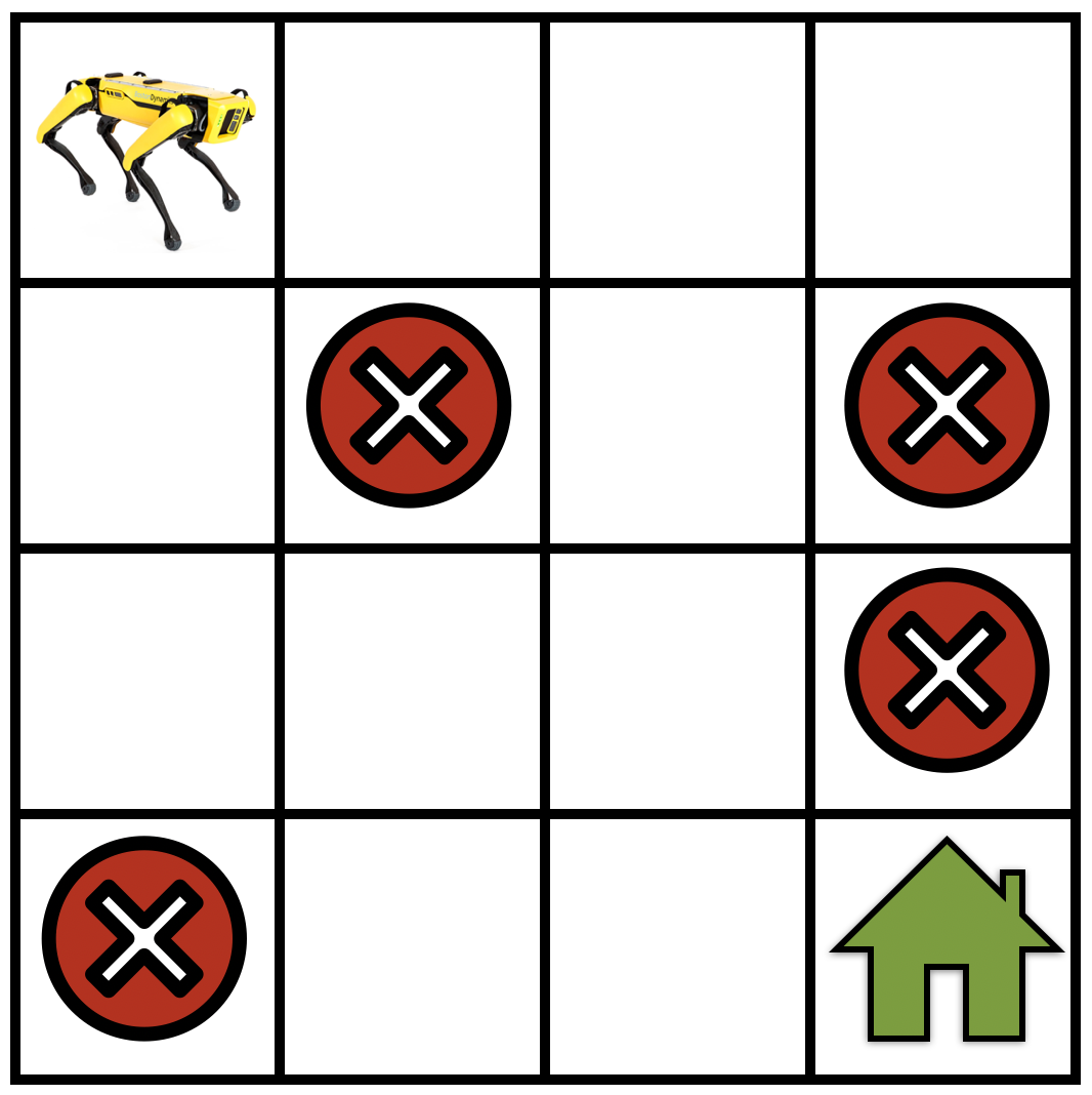
Fig. 17.1.1 A simple gridworld navigation task where the robot not only has to find its way to the goal location (shown as a green house) but also has to avoid trap locations (shown as red cross signs). 그림 17.1.1 로봇이 목표 위치(녹색 집으로 표시)로 가는 길을 찾아야 할 뿐만 아니라 트랩 위치(적십자 기호로 표시)를 피해야 하는 간단한 그리드월드 탐색 작업입니다.
LetSbe the set of states in the MDP. As a concrete example seeFig. 17.1.1, for a robot that is navigating a gridworld. In this case,Scorresponds to the set of locations that the robot can be at any given timestep.
S를 MDP의 상태 집합으로 설정합니다. 구체적인 예로 그리드 세계를 탐색하는 로봇에 대한 그림 17.1.1을 참조하세요. 이 경우 S는 주어진 시간 단계에서 로봇이 있을 수 있는 위치 집합에 해당합니다.
LetAbe the set of actions that the robot can take at each state, e.g., “go forward”, “turn right”, “turn left”, “stay at the same location”, etc. Actions can change the current state of the robot to some other state within the setS.
A를 로봇이 각 상태에서 취할 수 있는 일련의 작업(예: "앞으로 이동", "우회전", "좌회전", "같은 위치에 유지" 등)이라고 가정합니다. 작업은 로봇의 현재 상태를 변경할 수 있습니다. 로봇을 세트 S 내의 다른 상태로 전환합니다.
It may happen that we do not know how the robot movesexactlybut only know it up to some approximation. We model this situation in reinforcement learning as follows: if the robot takes an action “go forward”, there might be a small probability that it stays at the current state, another small probability that it “turns left”, etc. Mathematically, this amounts to defining a “transition function”T:S×A×S→[0,1]such thatT(s,a,s′)=P(s′∣s,a)using the conditional probability of reaching a state s′given that the robot was at statesand took an actiona. The transition function is a probability distribution and we therefore have∑s′∈s**T(s,a,s′)=1for alls∈Sanda∈A, i.e., the robot has to go to some state if it takes an action.
로봇이 정확히 어떻게 움직이는지는 모르지만 대략적인 정도까지만 알 수 있는 경우도 있습니다. 우리는 강화 학습에서 이 상황을 다음과 같이 모델링합니다. 로봇이 "앞으로 나아가는" 행동을 취하면 현재 상태에 머무를 확률이 작을 수도 있고 "좌회전"할 확률도 작을 수도 있습니다. 수학적으로 이는 상태에 도달할 조건부 확률을 사용하여 T(s,a,s')=P(s'∣s,a)가 되도록 "전이 함수" T:S×A×S→[0,1]을 정의하는 것과 같습니다. s' 로봇이 s 상태에 있고 조치를 취했다는 점을 고려하면 a. 전이 함수는 확률 분포이므로 모든 s∈S 및 a∈A에 대해 ∑s′∈s**T(s,a,s′)=1입니다. 즉, 로봇은 다음과 같은 경우 어떤 상태로 이동해야 합니다. 조치가 필요합니다.
We now construct a notion of which actions are useful and which ones are not using the concept of a “reward”r:S×A→ℝ. We say that the robot gets a rewardr(s,a)if the robot takes an actionaat states. If the rewardr(s,a)is large, this indicates that taking the actionaat statesis more useful to achieving the goal of the robot, i.e., going to the green house. If the rewardr(s,a)is small, then actionais less useful to achieving this goal. It is important to note that the reward is designed by the user (the person who creates the reinforcement learning algorithm) with the goal in mind.
이제 우리는 어떤 행동이 유용하고 어떤 행동이 "보상" r:S×A→ℝ 개념을 사용하지 않는지에 대한 개념을 구성합니다. 로봇이 상태 s에서 행동 a를 취하면 로봇은 보상 r(s,a)를 받는다고 말합니다. 보상 r(s,a)가 크다면, 이는 상태 s에서 a를 취하는 것이 로봇의 목표, 즉 온실로 가는 것을 달성하는 데 더 유용하다는 것을 나타냅니다. 보상 r(s,a)가 작으면 작업 a는 이 목표를 달성하는 데 덜 유용합니다. 보상은 목표를 염두에 두고 사용자(강화학습 알고리즘을 생성하는 사람)에 의해 설계된다는 점에 유의하는 것이 중요합니다.
17.1.2.Return and Discount Factor
The different components above together form a Markov decision process (MDP)
위의 다양한 구성 요소가 함께 MDP(Markov Decision Process)를 구성합니다.
Let’s now consider the situation when the robot starts at a particular states0∈Sand continues taking actions to result in a trajectory
이제 로봇이 특정 상태 s0∈S에서 시작하여 계속해서 궤적을 생성하는 작업을 수행하는 상황을 고려해 보겠습니다.
At each time steptthe robot is at a statestand takes an actionatwhich results in a rewardrt=r(st,at). Thereturnof a trajectory is the total reward obtained by the robot along such a trajectory
각 시간 단계 t에서 로봇은 상태 st에 있고 보상 rt=r(st,at)을 가져오는 작업을 수행합니다. 궤도의 복귀는 그러한 궤도를 따라 로봇이 얻는 총 보상입니다.
The goal in reinforcement learning is to find a trajectory that has the largestreturn.
강화학습의 목표는 가장 큰 수익을 내는 궤적을 찾는 것입니다.
Think of the situation when the robot continues to travel in the gridworld without ever reaching the goal location. The sequence of states and actions in a trajectory can be infinitely long in this case and thereturnof any such infinitely long trajectory will be infinite. In order to keep the reinforcement learning formulation meaningful even for such trajectories, we introduce the notion of a discount factorγ<1. We write the discountedreturnas
로봇이 목표 위치에 도달하지 못한 채 그리드 세계에서 계속 이동하는 상황을 생각해 보세요. 이 경우 궤도의 상태와 동작의 순서는 무한히 길어질 수 있으며 무한히 긴 궤도의 반환은 무한합니다. 그러한 궤적에 대해서도 강화 학습 공식을 의미 있게 유지하기 위해 할인 계수 γ<1이라는 개념을 도입합니다. 우리는 할인된 수익을 다음과 같이 씁니다.
Note that ifγis very small, the rewards earned by the robot in the far future, sayt=1000, are heavily discounted by the factorγ**1000. This encourages the robot to select short trajectories that achieve its goal, namely that of going to the green house in the gridwold example (seeFig. 17.1.1). For large values of the discount factor, sayγ=0.99, the robot is encouraged toexploreand then find the best trajectory to go to the goal location.
γ가 매우 작은 경우, 먼 미래에 로봇이 얻는 보상(t=1000)은 γ**1000 인자로 크게 할인됩니다. 이는 로봇이 목표를 달성하는 짧은 궤적, 즉 그리드월드 예에서 온실로 가는 경로를 선택하도록 장려합니다(그림 17.1.1 참조). 할인 요소의 큰 값(γ=0.99라고 가정)의 경우 로봇은 목표 위치로 이동하기 위한 최적의 궤적을 탐색하고 찾도록 권장됩니다.
17.1.3.Discussion of the Markov Assumption
Let us think of a new robot where the statestis the location as above but the actionatis the acceleration that the robot applies to its wheels instead of an abstract command like “go forward”. If this robot has some non-zero velocity at statest, then the next locationst+1is a function of the past locationst, the accelerationat, also the velocity of the robot at timetwhich is proportional tost−st−1. This indicates that we should have
위와 같이 상태 st가 위치이지만 동작은 "전진"과 같은 추상적인 명령 대신 로봇이 바퀴에 적용하는 가속도인 새로운 로봇을 생각해 보겠습니다. 이 로봇이 상태 st에서 0이 아닌 속도를 갖는 경우 다음 위치 st+1은 과거 위치 st의 함수, 가속도, st−st−에 비례하는 시간 t에서의 로봇 속도의 함수입니다. 1. 이는 우리가 이것을 가져야 함을 나타냅니다.
the “some function” in our case would be Newton’s law of motion. This is quite different from our transition function that simply depends uponstandat.
우리의 경우 "some function"은 뉴턴의 운동 법칙이 될 것입니다. 이는 단순히 st와 at에 의존하는 전환 함수와는 상당히 다릅니다.
Markov systems are all systems where the next statest+1is only a function of the current statestand the actionαttaken at the current state. In Markov systems, the next state does not depend on which actions were taken in the past or the states that the robot was at in the past. For example, the new robot that has acceleration as the action above is not Markovian because the next locationst+1depends upon the previous statest−1through the velocity. It may seem that Markovian nature of a system is a restrictive assumption, but it is not so. Markov Decision Processes are still capable of modeling a very large class of real systems. For example, for our new robot, if we chose our statestto the tuple(location,velocity)then the system is Markovian because its next state(location t+1,velocity t+1)depends only upon the current state(location t,velocity t)and the action at the current stateαt.
마르코프 시스템은 다음 상태 st+1이 현재 상태 st와 현재 상태에서 취한 조치 αt의 함수일 뿐인 모든 시스템입니다. Markov 시스템에서 다음 상태는 과거에 어떤 작업이 수행되었는지 또는 로봇이 과거에 있었던 상태에 의존하지 않습니다. 예를 들어, 위의 동작으로 가속도를 갖는 새 로봇은 다음 위치 st+1이 속도를 통해 이전 상태 st-1에 의존하기 때문에 Markovian이 아닙니다. 시스템의 마코브적 특성은 제한적인 가정인 것처럼 보일 수 있지만 그렇지 않습니다. Markov 결정 프로세스는 여전히 매우 큰 규모의 실제 시스템을 모델링할 수 있습니다. 예를 들어, 새 로봇의 경우 상태 st를 튜플(위치, 속도)로 선택하면 다음 상태(위치 t+1, 속도 t+1)가 현재 상태(위치)에만 의존하기 때문에 시스템은 마코비안입니다. t,속도 t) 및 현재 상태에서의 작용 αt.
17.1.4.Summary
The reinforcement learning problem is typically modeled using Markov Decision Processes. A Markov decision process (MDP) is defined by a tuple of four entities(S,A,T,r)whereSis the state space,Ais the action space,Tis the transition function that encodes the transition probabilities of the MDP andris the immediate reward obtained by taking action at a particular state.
강화 학습 문제는 일반적으로 Markov 결정 프로세스를 사용하여 모델링됩니다. 마르코프 결정 프로세스(MDP)는 4개 엔터티(S,A,T,r)의 튜플로 정의됩니다. 여기서 S는 상태 공간, A는 작업 공간, T는 MDP의 전환 확률을 인코딩하는 전환 함수입니다. r은 특정 상태에서 조치를 취함으로써 얻은 즉각적인 보상입니다.
17.1.5.Exercises
Suppose that we want to design an MDP to modelMountainCarproblem.
What would be the set of states?
What would be the set of actions?
What would be the possible reward functions?
How would you design an MDP for an Atari game likePong game?
Pratik Chaudhari(University of Pennsylvania and Amazon),Rasool Fakoor(Amazon), andKavosh Asadi(Amazon)
Reinforcement Learning (RL) is a suite of techniques that allows us to build machine learning systems that take decisions sequentially. For example, a package containing new clothes that you purchased from an online retailer arrives at your doorstep after a sequence of decisions, e.g., the retailer finding the clothes in the warehouse closest to your house, putting the clothes in a box, transporting the box via land or by air, and delivering it to your house within the city. There are many variables that affect the delivery of the package along the way, e.g., whether or not the clothes were available in the warehouse, how long it took to transport the box, whether it arrived in your city before the daily delivery truck left, etc. The key idea is that at each stage these variables that we do not often control affect the entire sequence of events in the future, e.g., if there were delays in packing the box in the warehouse the retailer may need to send the package via air instead of ground to ensure a timely delivery. Reinforcement Learning methods allow us to take the appropriate action at each stage of a sequential decision making problem in order to maximize some utility eventually, e.g., the timely delivery of the package to you.
강화 학습(RL)은 순차적으로 결정을 내리는 기계 학습 시스템을 구축할 수 있는 기술 모음입니다. 예를 들어, 온라인 소매점에서 구입한 새 옷이 들어 있는 패키지는 소매점이 집에서 가장 가까운 창고에서 옷을 찾고, 옷을 상자에 넣고, 상자를 운반하는 등 일련의 결정을 거쳐 문앞에 도착합니다. 육로나 항공으로 도시 내 집까지 배달해 드립니다. 도중에 패키지 배송에 영향을 미치는 많은 변수가 있습니다. 예를 들어 창고에 옷이 있는지 여부, 상자를 운송하는 데 걸리는 시간, 일일 배달 트럭이 떠나기 전에 상자가 도시에 도착했는지 여부 등이 있습니다. 핵심 아이디어는 각 단계에서 우리가 자주 제어하지 않는 이러한 변수가 미래의 전체 이벤트 순서에 영향을 미친다는 것입니다. 예를 들어, 창고에서 상자를 포장하는 데 지연이 발생한 경우 소매업체는 적시 배송을 보장하기 위해 육상 대신 항공을 통해 패키지를 보내야 할 수도 있습니다. 강화 학습 방법을 사용하면 궁극적으로 패키지를 적시에 전달하는 등 일부 유틸리티를 최대화하기 위해 순차적 의사 결정 문제의 각 단계에서 적절한 조치를 취할 수 있습니다.
Such sequential decision making problems are seen in numerous other places, e.g., while playingGoyour current move determines the next moves and the opponent’s moves are the variables that you cannot control… a sequence of moves eventually determines whether or not you win; the movies that Netflix recommends to you now determine what you watch, whether you like the movie or not is unknown to Netflix, eventually a sequence of movie recommendations determines how satisfied you are with Netflix. Reinforcement learning is being used today to develop effective solutions to these problems(Mnihet al., 2013,Silveret al., 2016). The key distinction between reinforcement learning and standard deep learning is that in standard deep learning the prediction of a trained model on one test datum does not affect the predictions on a future test datum; in reinforcement learning decisions at future instants (in RL, decisions are also called actions) are affected by what decisions were made in the past.
이러한 순차적 의사 결정 문제는 다른 여러 곳에서 볼 수 있습니다. 예를 들어 바둑을 플레이하는 동안 현재 동작이 다음 동작을 결정하고 상대방의 동작은 제어할 수 없는 변수입니다. 일련의 동작이 결국 승리 여부를 결정합니다. 이제 Netflix가 추천하는 영화가 무엇을 시청할지 결정합니다. 영화를 좋아하는지 여부는 Netflix에 알려지지 않으며 결국 일련의 영화 추천에 따라 Netflix에 대한 만족도가 결정됩니다. 오늘날 강화 학습은 이러한 문제에 대한 효과적인 솔루션을 개발하는 데 사용되고 있습니다(Mnih et al., 2013, Silver et al., 2016). 강화 학습과 표준 딥 러닝의 주요 차이점은 표준 딥 러닝에서 하나의 테스트 데이터에 대한 훈련된 모델 예측이 향후 테스트 데이터에 대한 예측에 영향을 미치지 않는다는 것입니다. 강화 학습에서 미래 순간의 결정(RL에서는 결정이라고도 함)은 과거에 내려진 결정에 영향을 받습니다.
In this chapter, we will develop the fundamentals of reinforcement learning and obtain hands-on experience in implementing some popular reinforcement learning methods. We will first develop a concept called a Markov Decision Process (MDP) which allows us to think of such sequential decision making problems. An algorithm called Value Iteration will be our first insight into solving reinforcement learning problems under the assumption that we know how the uncontrolled variables in an MDP (in RL, these controlled variables are called the environment) typically behave. Using the more general version of Value Iteration, an algorithm called Q-Learning, we will be able to take appropriate actions even when we do not necessarily have full knowledge of the environment. We will then study how to use deep networks for reinforcement learning problems by imitating the actions of an expert. And finally, we will develop a reinforcement learning method that uses a deep network to take actions in unknown environments. These techniques form the basis of more advanced RL algorithms that are used today in a variety of real-world applications, some of which we will point to in the chapter.
이 장에서는 강화 학습의 기본 사항을 개발하고 몇 가지 널리 사용되는 강화 학습 방법을 구현하는 실습 경험을 얻을 것입니다. 우리는 먼저 이러한 순차적 의사결정 문제를 생각할 수 있게 해주는 Markov Decision Process(MDP)라는 개념을 개발할 것입니다. Value Iteration이라는 알고리즘은 MDP(RL에서는 이러한 제어 변수를 환경이라고 함)의 제어되지 않은 변수가 일반적으로 어떻게 동작하는지 알고 있다는 가정 하에 강화 학습 문제를 해결하기 위한 첫 번째 통찰력이 될 것입니다. Q-Learning이라는 알고리즘인 Value Iteration의 보다 일반적인 버전을 사용하면 환경에 대한 완전한 지식이 없어도 적절한 조치를 취할 수 있습니다. 그런 다음 전문가의 행동을 모방하여 강화 학습 문제에 딥 네트워크를 사용하는 방법을 연구합니다. 그리고 마지막으로 딥 네트워크를 활용하여 알려지지 않은 환경에서 조치를 취하는 강화학습 방법을 개발하겠습니다. 이러한 기술은 오늘날 다양한 실제 애플리케이션에서 사용되는 고급 RL 알고리즘의 기초를 형성하며, 그 중 일부는 이 장에서 언급할 것입니다.
Markov Decision Process(MDP)란?
'마르코프 결정 과정' 또는 'Markov Decision Process (MDP)'는 강화 학습(Reinforcement Learning)과 관련된 수학적 모델 및 프레임워크입니다. MDP는 시간 단계(time step)별로 에이전트가 환경과 상호 작용하는 상황을 수학적으로 모델링하는 데 사용됩니다.
MDP는 다음과 같은 구성 요소로 정의됩니다:
상태(State): 에이전트가 존재하는 시스템의 현재 상태를 나타내는 값 또는 변수입니다. 이러한 상태는 모든 정보를 포함하며, 에이전트의 의사 결정에 영향을 미칩니다.
행동(Action): 에이전트가 선택할 수 있는 가능한 행동 또는 행동의 집합입니다. 행동은 에이전트가 상태를 변경하거나 환경에 영향을 주는 방법입니다.
보상(Reward): 각 상태에서 에이전트가 수행한 행동에 대한 즉각적인 피드백으로, 보상은 얼마나 좋은지 또는 나쁜지를 나타냅니다. 에이전트의 목표는 미래 보상의 합을 최대화하는 것입니다.
상태 전이 확률(Transition Probability): 에이전트가 특정 상태에서 특정 행동을 선택할 때, 다음 상태로 이동할 확률을 나타냅니다. 이것은 환경의 동적인 특성을 모델링하는 데 사용됩니다.
감쇠 계수(Discount Factor): 미래 보상의 현재 가치를 조절하는 매개변수로, 미래 보상에 대한 중요성을 나타냅니다.
MDP는 에이전트가 현재 상태에서 어떤 행동을 선택할지, 그 선택에 따른 보상을 최대화하기 위한 정책(Policy)을 학습하는 문제를 다룹니다. 최적의 정책은 최대 보상을 얻기 위한 행동 선택 전략입니다.
MDP는 강화 학습 문제를 정형화하고 수학적으로 해결 가능한 형태로 만들어주므로, 다양한 환경에서 에이전트의 학습과 의사 결정을 모델링하는 데 사용됩니다.
Fig. 17.1 Reinforcement Learning Structure
Reinforcement learning이란?
강화 학습(Reinforcement Learning)은 기계 학습의 한 분야로, 특정 환경 내에서 에이전트(Agent)가 어떤 일련의 행동을 수행하여 보상을 최대화하는 방법을 학습하는 프레임워크입니다. 이러한 환경은 주로 문제 해결에 관련되며, 강화 학습 에이전트는 환경과 상호작용하면서 다양한 상황에서 어떤 행동을 선택해야 하는지를 학습합니다.
강화 학습의 주요 구성 요소는 다음과 같습니다:
에이전트(Agent): 학습하는 주체로, 의사 결정을 내리고 행동을 수행합니다. 이 에이전트는 주어진 상황에서 보상을 최대화하기 위한 최적의 행동을 찾아내는 것이 목표입니다.
환경(Environment): 에이전트가 상호작용하는 대상으로, 문제의 성격에 따라 다양한 형태를 가질 수 있습니다. 환경은 에이전트의 행동에 따라 변화하며, 행동에 대한 응답으로 보상을 제공합니다.
상태(State): 환경의 특정 순간 상태를 나타내는 정보입니다. 에이전트는 주어진 상태에서 어떤 행동을 선택해야 하는지 결정합니다.
행동(Action): 에이전트가 환경에서 수행하는 행동 또는 의사 결정을 나타냅니다. 각 상태에서 가능한 행동의 집합이 정의되며, 에이전트는 이 중에서 하나를 선택합니다.
보상(Reward): 에이전트의 행동에 대한 피드백으로, 주어진 행동이 얼마나 좋은지 또는 나쁜지를 나타냅니다. 목표는 보상을 최대화하는 행동을 선택하는 것입니다.
강화 학습의 핵심 과제는 에이전트가 주어진 환경에서 최적의 정책(Policy)을 학습하는 것입니다. 정책은 상태에 따라 에이전트가 어떤 행동을 선택해야 하는지를 결정하는 전략을 의미합니다. 에이전트는 다양한 정책을 시도하고 보상을 통해 피드백을 받으며 점차적으로 최적의 정책을 발견합니다.
강화 학습은 로봇 제어, 게임 플레이, 자율 주행 자동차, 자연어 처리 및 금융 등 다양한 응용 분야에서 사용됩니다. 주어진 환경에서 최적의 행동을 결정하는 방법을 학습함으로써 문제를 해결하는 데 활용됩니다.