
https://d2l.ai/chapter_reinforcement-learning/qlearning.html
17.3. Q-Learning — Dive into Deep Learning 1.0.3 documentation
d2l.ai
17.3. Q-Learning
In the previous section, we discussed the Value Iteration algorithm which requires accessing the complete Markov decision process (MDP), e.g., the transition and reward functions. In this section, we will look at Q-Learning (Watkins and Dayan, 1992) which is an algorithm to learn the value function without necessarily knowing the MDP. This algorithm embodies the central idea behind reinforcement learning: it will enable the robot to obtain its own data.
이전 섹션에서는 전체 마르코프 결정 프로세스(MDP)(예: 전환 및 보상 기능)에 액세스해야 하는 Value Iteration 알고리즘에 대해 논의했습니다. 이번 절에서는 MDP를 알지 못하는 상태에서 가치함수를 학습하는 알고리즘인 Q-Learning(Watkins and Dayan, 1992)을 살펴보겠습니다. 이 알고리즘은 강화 학습의 핵심 아이디어를 구현합니다. 이를 통해 로봇은 자체 데이터를 얻을 수 있습니다.
Q-Learning이란?
'Q-Learning'은 강화 학습(Reinforcement Learning)에서 사용되는 강화 학습 알고리즘 중 하나입니다. Q-Learning은 미래 보상을 고려하여 에이전트가 최적의 행동을 학습하는 데 사용됩니다.
Q-Learning의 주요 아이디어는 'Q-Value' 또는 'Action-Value' 함수를 학습하는 것입니다. 각 상태(State) 및 행동(Action)에 대한 Q-Value는 해당 상태에서 특정 행동을 선택했을 때 얻을 수 있는 예상 보상의 합계를 나타냅니다. Q-Value 함수는 다음과 같이 정의됩니다.
Q(s, a) = (1 - α) * Q(s, a) + α * (R + γ * max(Q(s', a')))
여기서:
- Q(s, a): 상태 s에서 행동 a를 선택할 때의 Q-Value입니다.
- α(알파): 학습률(learning rate)로, Q-Value를 업데이트할 때 현재 값과 새로운 값을 얼마나 가중치를 두고 합칠지 결정합니다.
- R: 현재 상태에서 행동을 수행했을 때 얻는 보상(reward)입니다.
- γ(감마): 감쇠 계수(discount factor)로, 미래 보상을 현재 보상보다 얼마나 가치 있게 여길지를 결정합니다.
- max(Q(s', a')): 다음 상태 s'에서 가능한 모든 행동 중에서 최대 Q-Value를 선택합니다.
Q-Learning 알고리즘의 주요 특징은 다음과 같습니다:
- 모델-Fee: 환경에 대한 사전 지식 없이 직접 경험을 통해 학습합니다.
- Off-Policy: 정책(policy)을 따라가는 것이 아니라, 최적의 정책을 찾기 위해 여러 정책을 시도하면서 학습합니다.
- 탐험(Exploration)과 이용(Exploitation)의 균형: Q-Learning은 탐험을 통해 더 나은 행동을 찾으며, 이용을 통해 현재까지 학습된 지식을 활용합니다.
Q-Learning은 강화 학습의 고전적인 알고리즘 중 하나로, 다양한 응용 분야에서 사용됩니다. 특히, 게임이나 로봇 제어와 같은 영역에서 많이 활용되며, 강화 학습의 핵심 개념을 이해하는 데 도움이 됩니다.
17.3.1. The Q-Learning Algorithm
Recall that value iteration for the action-value function in Value Iteration corresponds to the update
Value Iteration에서 action-value function에 대한 value iteration은 업데이트에 해당한다는 점을 기억하세요.

As we discussed, implementing this algorithm requires knowing the MDP, specifically the transition function P(s′∣s,a). The key idea behind Q-Learning is to replace the summation over all s′∈S in the above expression by a summation over the states visited by the robot. This allows us to subvert the need to know the transition function.
논의한 대로 이 알고리즘을 구현하려면 MDP, 특히 전이 함수 P(s′∣s,a)를 알아야 합니다. Q-Learning의 핵심 아이디어는 위 표현식의 모든 s′∈S에 대한 합산을 로봇이 방문한 상태에 대한 합산으로 대체하는 것입니다. 이를 통해 우리는 전환 함수를 알아야 할 필요성을 뒤집을 수 있습니다.
17.3.2. An Optimization Problem Underlying Q-Learning
Let us imagine that the robot uses a policy πe(a∣s) to take actions. Just like the previous chapter, it collects a dataset of n trajectories of T timesteps each {(s**i t,a**i t)t=0,…,T−1}i=1,…,n. Recall that value iteration is really a set of constraints that ties together the action-value Q*(s,a) of different states and actions to each other. We can implement an approximate version of value iteration using the data that the robot has collected using πe as
로봇이 정책 πe(a∣s)를 사용하여 조치를 취한다고 가정해 보겠습니다. 이전 장과 마찬가지로 각 {(s**i t,a**i t)t=0,…,T−1}i=1,…,n T 시간 단계의 n 궤적 데이터 세트를 수집합니다. value iteration은 실제로 서로 다른 상태와 동작의 동작 값 Q*(s,a)를 서로 연결하는 제약 조건 집합이라는 점을 기억하세요. 로봇이 πe를 사용하여 수집한 데이터를 사용하여 대략적인 value iteration 버전을 구현할 수 있습니다.

Let us first observe the similarities and differences between this expression and value iteration above. If the robot’s policy πe were equal to the optimal policy π*, and if it collected an infinite amount of data, then this optimization problem would be identical to the optimization problem underlying value iteration. But while value iteration requires us to know P(s′∣s,a), the optimization objective does not have this term. We have not cheated: as the robot uses the policy πe to take an action a**i t at state s**i t, the next state s**i t+1 is a sample drawn from the transition function. So the optimization objective also has access to the transition function, but implicitly in terms of the data collected by the robot.
먼저 이 표현과 위의 값 반복 간의 유사점과 차이점을 살펴보겠습니다. 로봇의 정책 πe가 최적 정책 π*와 같고 무한한 양의 데이터를 수집했다면 이 최적화 문제는 가치 반복의 기본이 되는 최적화 문제와 동일할 것입니다. 그러나 값 반복을 위해서는 P(s′∣s,a)를 알아야 하지만 최적화 목적에는 이 항이 없습니다. 우리는 속이지 않았습니다. 로봇이 상태 s**i t에서 a**i t 작업을 수행하기 위해 정책 πe를 사용하므로 다음 상태 s**i t+1은 전이 함수에서 가져온 샘플입니다. 따라서 최적화 목표도 전환 기능에 액세스할 수 있지만 암시적으로 로봇이 수집한 데이터 측면에서 접근할 수 있습니다.
The variables of our optimization problem are Q(s,a) for all s∈S and a∈A. We can minimize the objective using gradient descent. For every pair (s**i t,a**i t) in our dataset, we can write
최적화 문제의 변수는 모든 s∈S 및 a∈A에 대한 Q(s,a)입니다. 경사 하강을 사용하여 목표를 최소화할 수 있습니다. 데이터 세트의 모든 쌍(s**i t,a**i t)에 대해 다음과 같이 쓸 수 있습니다.

where α is the learning rate. Typically in real problems, when the robot reaches the goal location, the trajectories end. The value of such a terminal state is zero because the robot does not take any further actions beyond this state. We should modify our update to handle such states as
여기서 α는 학습률입니다. 일반적으로 실제 문제에서는 로봇이 목표 위치에 도달하면 궤도가 종료됩니다. 로봇이 이 상태를 넘어서는 추가 작업을 수행하지 않기 때문에 이러한 최종 상태의 값은 0입니다. 다음과 같은 상태를 처리하려면 업데이트를 수정해야 합니다.

where 𝟙 s**i t+1 is terminal is an indicator variable that is one if s**i t+1 is a terminal state and zero otherwise. The value of state-action tuples (s,a) that are not a part of the dataset is set to −∞. This algorithm is known as Q-Learning.
여기서 𝟙 s**i t+1 is 터미널은 s**i t+1이 터미널 상태이면 1이고 그렇지 않으면 0인 표시 변수입니다. 데이터세트의 일부가 아닌 상태-동작 튜플(s,a)의 값은 −무효로 설정됩니다. 이 알고리즘은 Q-Learning으로 알려져 있습니다.
Given the solution of these updates Q^, which is an approximation of the optimal value function Q*, we can obtain the optimal deterministic policy corresponding to this value function easily using
최적의 가치 함수 Q*의 근사치인 이러한 업데이트 Q^의 솔루션이 주어지면 다음을 사용하여 이 가치 함수에 해당하는 최적의 결정론적 정책을 쉽게 얻을 수 있습니다.

There can be situations when there are multiple deterministic policies that correspond to the same optimal value function; such ties can be broken arbitrarily because they have the same value function.
동일한 최적 가치 함수에 해당하는 여러 결정론적 정책이 있는 상황이 있을 수 있습니다. 이러한 관계는 동일한 가치 함수를 갖기 때문에 임의로 끊어질 수 있습니다.
17.3.3. Exploration in Q-Learning
The policy used by the robot to collect data πe is critical to ensure that Q-Learning works well. Afterall, we have replaced the expectation over s′ using the transition function P(s′∣s,a) using the data collected by the robot. If the policy πe does not reach diverse parts of the state-action space, then it is easy to imagine our estimate Q^ will be a poor approximation of the optimal Q*. It is also important to note that in such a situation, the estimate of Q* at all states s∈S will be bad, not just the ones visited by πe. This is because the Q-Learning objective (or value iteration) is a constraint that ties together the value of all state-action pairs. It is therefore critical to pick the correct policy πe to collect data.
Q-Learning이 제대로 작동하려면 로봇이 데이터 πe를 수집하는 데 사용하는 정책이 중요합니다. 결국 우리는 로봇이 수집한 데이터를 사용하여 전이 함수 P(s′∣s,a)를 사용하여 s′에 대한 기대값을 대체했습니다. 정책 πe가 상태-행동 공간의 다양한 부분에 도달하지 못한다면 우리의 추정치 Q^가 최적 Q*에 대한 잘못된 근사치일 것이라고 상상하기 쉽습니다. 그러한 상황에서는 πe가 방문한 상태뿐만 아니라 모든 상태 s∈S에서 Q*의 추정값이 나쁠 것이라는 점에 유의하는 것도 중요합니다. 이는 Q-Learning 목표(또는 값 반복)가 모든 상태-작업 쌍의 값을 하나로 묶는 제약 조건이기 때문입니다. 따라서 데이터를 수집하기 위해 올바른 정책을 선택하는 것이 중요합니다.
We can mitigate this concern by picking a completely random policy πe that samples actions uniformly randomly from A. Such a policy would visit all states, but it will take a large number of trajectories before it does so.
우리는 A에서 균일하게 무작위로 작업을 샘플링하는 완전히 무작위적인 정책 πe를 선택하여 이러한 우려를 완화할 수 있습니다. 이러한 정책은 모든 상태를 방문하지만 그렇게 하기 전에 많은 수의 궤적을 필요로 합니다.
We thus arrive at the second key idea in Q-Learning, namely exploration. Typical implementations of Q-Learning tie together the current estimate of Q and the policy πe to set

where ε is called the “exploration parameter” and is chosen by the user. The policy πe is called an exploration policy. This particular πe is called an ε-greedy exploration policy because it chooses the optimal action (under the current estimate Q^) with probability 1−ε but explores randomly with the remainder probability ε. We can also use the so-called softmax exploration policy
여기서 ε는 "탐색 매개변수"라고 하며 사용자가 선택합니다. 정책 πe를 탐사 정책이라고 합니다. 이 특정 πe는 확률 1−ε로 최적의 행동(현재 추정치 Q^ 하에서)을 선택하지만 나머지 확률 ε으로 무작위로 탐색하기 때문에 ε-탐욕 탐색 정책이라고 합니다. 소위 소프트맥스 탐색 정책을 사용할 수도 있습니다.
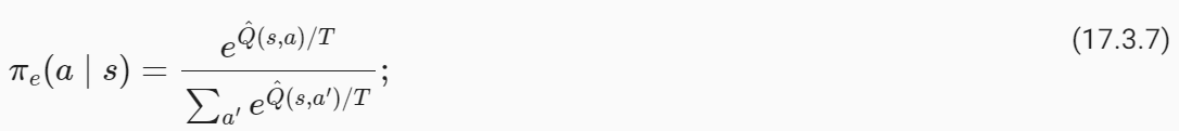
where the hyper-parameter T is called temperature. A large value of ε in ε-greedy policy functions similarly to a large value of temperature T for the softmax policy.
여기서 초매개변수 T를 온도라고 합니다. ε-탐욕 정책에서 ε의 큰 값은 소프트맥스 정책의 온도 T의 큰 값과 유사하게 기능합니다.
It is important to note that when we pick an exploration that depends upon the current estimate of the action-value function Q^, we need to resolve the optimization problem periodically. Typical implementations of Q-Learning make one mini-batch update using a few state-action pairs in the collected dataset (typically the ones collected from the previous timestep of the robot) after taking every action using πe.
행동-가치 함수 Q^의 현재 추정에 의존하는 탐색을 선택할 때 최적화 문제를 주기적으로 해결해야 한다는 점에 유의하는 것이 중요합니다. Q-Learning의 일반적인 구현은 πe를 사용하여 모든 작업을 수행한 후 수집된 데이터 세트(일반적으로 로봇의 이전 단계에서 수집된 데이터)의 몇 가지 상태-작업 쌍을 사용하여 하나의 미니 배치 업데이트를 수행합니다.
17.3.4. The “Self-correcting” Property of Q-Learning
The dataset collected by the robot during Q-Learning grows with time. Both the exploration policy πe and the estimate Q^ evolve as the robot collects more data. This gives us a key insight into why Q-Learning works well. Consider a state s: if a particular action a has a large value under the current estimate Q^(s,a), then both the ε-greedy and the softmax exploration policies have a larger probability of picking this action. If this action actually is not the ideal action, then the future states that arise from this action will have poor rewards. The next update of the Q-Learning objective will therefore reduce the value Q^(s,a), which will reduce the probability of picking this action the next time the robot visits state s. Bad actions, e.g., ones whose value is overestimated in Q^(s,a), are explored by the robot but their value is correct in the next update of the Q-Learning objective. Good actions, e.g., whose value Q^(s,a) is large, are explored more often by the robot and thereby reinforced. This property can be used to show that Q-Learning can converge to the optimal policy even if it begins with a random policy πe (Watkins and Dayan, 1992).
Q-Learning 중에 로봇이 수집한 데이터 세트는 시간이 지남에 따라 증가합니다. 탐색 정책 πe와 추정치 Q^는 모두 로봇이 더 많은 데이터를 수집함에 따라 진화합니다. 이는 Q-Learning이 왜 잘 작동하는지에 대한 중요한 통찰력을 제공합니다. 상태 s를 고려하십시오. 특정 작업 a가 현재 추정치 Q^(s,a)보다 큰 값을 갖는 경우 ε-탐욕 및 소프트맥스 탐색 정책 모두 이 작업을 선택할 확률이 더 높습니다. 만약 이 행동이 실제로 이상적인 행동이 아니라면, 이 행동에서 발생하는 미래 상태는 낮은 보상을 받게 될 것입니다. 따라서 Q-Learning 목표의 다음 업데이트는 Q^(s,a) 값을 줄여 로봇이 다음에 상태 s를 방문할 때 이 작업을 선택할 확률을 줄입니다. 나쁜 행동, 예를 들어 Q^(s,a)에서 값이 과대평가된 행동은 로봇에 의해 탐색되지만 그 값은 Q-Learning 목표의 다음 업데이트에서 정확합니다. 예를 들어 Q^(s,a) 값이 큰 좋은 행동은 로봇에 의해 더 자주 탐색되어 강화됩니다. 이 속성은 Q-Learning이 무작위 정책 πe로 시작하더라도 최적의 정책으로 수렴할 수 있음을 보여주는 데 사용될 수 있습니다(Watkins and Dayan, 1992).
This ability to not only collect new data but also collect the right kind of data is the central feature of reinforcement learning algorithms, and this is what distinguishes them from supervised learning. Q-Learning, using deep neural networks (which we will see in the DQN chapeter later), is responsible for the resurgence of reinforcement learning (Mnih et al., 2013).
새로운 데이터를 수집할 뿐만 아니라 올바른 종류의 데이터를 수집하는 이러한 능력은 강화 학습 알고리즘의 핵심 기능이며 지도 학습과 구별됩니다. 심층 신경망(나중에 DQN 장에서 볼 예정)을 사용하는 Q-Learning은 강화 학습의 부활을 담당합니다(Mnih et al., 2013).
17.3.5. Implementation of Q-Learning
We now show how to implement Q-Learning on FrozenLake from Open AI Gym. Note this is the same setup as we consider in Value Iteration experiment.
이제 Open AI Gym의 FrozenLake에서 Q-Learning을 구현하는 방법을 보여줍니다. 이는 Value Iteration 실험에서 고려한 것과 동일한 설정입니다.
%matplotlib inline
import random
import numpy as np
from d2l import torch as d2l

seed = 0  # Random number generator seed
gamma = 0.95  # Discount factor
num_iters = 256  # Number of iterations
alpha   = 0.9  # Learing rate
epsilon = 0.9  # Epsilon in epsilion gready algorithm
random.seed(seed)  # Set the random seed
np.random.seed(seed)

# Now set up the environment
env_info = d2l.make_env('FrozenLake-v1', seed=seed)
이 코드는 강화 학습 문제를 해결하기 위한 환경 설정을 합니다. 구체적으로는 FrozenLake-v1 환경에서 Q-Learning 알고리즘을 실행하기 위한 환경을 설정하는 부분입니다. 코드의 주요 요소를 설명하겠습니다.
- %matplotlib inline: 이 라인은 주피터 노트북(Jupyter Notebook)에서 그래프 및 플롯을 인라인으로 표시하도록 지시합니다.
- import random: 파이썬의 random 모듈을 가져옵니다. 이 모듈은 난수 생성과 관련된 함수를 제공합니다.
- import numpy as np: NumPy 라이브러리를 가져옵니다. NumPy는 과학적 계산을 위한 파이썬 라이브러리로, 다차원 배열과 관련된 기능을 제공합니다. 주로 행렬 연산과 숫자 계산에 사용됩니다.
- from d2l import torch as d2l: "d2l" 패키지에서 "torch" 모듈을 가져와서 "d2l"로 별명을 붙입니다. 이 패키지는 "Dive into Deep Learning" 책의 코드와 유틸리티 함수를 제공합니다.
- seed = 0: 랜덤 시드(seed)를 0으로 설정합니다. 시드를 설정하면 랜덤 함수 호출 결과가 항상 동일하게 유지됩니다. 이렇게 하면 실험의 재현성을 확보할 수 있습니다.
- gamma = 0.95: 감쇠 요인(gamma)을 설정합니다. 감쇠 요인은 미래 보상의 가치를 현재 보상의 가치보다 얼마나 가중치를 둘 것인지 결정하는 요소입니다.
- num_iters = 256: Q-Learning의 반복 횟수를 설정합니다. 즉, 학습을 몇 번 반복할 것인지를 결정합니다.
- alpha = 0.9: 학습률(learning rate)을 설정합니다. 학습률은 Q-Value를 업데이트할 때 현재 값과 새로운 값을 얼마나 가중치를 두고 합칠지를 결정하는 요소입니다.
- epsilon = 0.9: 엡실론(epsilon) 값을 설정합니다. 엡실론은 엡실론-그리디(epsilon-greedy) 알고리즘에서 사용되며, 탐험(Exploration)과 이용(Exploitation) 사이의 균형을 조절하는 역할을 합니다.
- random.seed(seed), np.random.seed(seed): 랜덤 시드를 설정하여 실험 결과의 재현성을 확보합니다. 같은 시드를 사용하면 같은 조건에서 항상 같은 결과를 얻을 수 있습니다.
- env_info = d2l.make_env('FrozenLake-v1', seed=seed): 'FrozenLake-v1'이라는 환경을 생성하고, 시드(seed)를 설정합니다. FrozenLake-v1은 강화 학습을 위한 환경으로, 얼어붙은 호수에서 목표 지점까지 에이전트를 이동시키는 과제를 제공합니다.
이제 이 설정된 환경에서 Q-Learning 알고리즘을 실행할 수 있습니다.
In the FrozenLake environment, the robot moves on a 4×4 grid (these are the states) with actions that are “up” (↑), “down” (→), “left” (←), and “right” (→). The environment contains a number of holes (H) cells and frozen (F) cells as well as a goal cell (G), all of which are unknown to the robot. To keep the problem simple, we assume the robot has reliable actions, i.e. P(s′∣s,a)=1 for all s∈S,a∈A. If the robot reaches the goal, the trial ends and the robot receives a reward of 1 irrespective of the action; the reward at any other state is 0 for all actions. The objective of the robot is to learn a policy that reaches the goal location (G) from a given start location (S) (this is s0) to maximize the return.
FrozenLake 환경에서 로봇은 "위"(↑), "아래"(→), "왼쪽"(←), "오른쪽"( →). 환경에는 다수의 구멍(H) 세포와 동결(F) 세포 및 목표 세포(G)가 포함되어 있으며, 이들 모두는 로봇에 알려지지 않습니다. 문제를 단순하게 유지하기 위해 로봇이 신뢰할 수 있는 동작을 한다고 가정합니다. 즉, 모든 s∈S,a∈A에 대해 P(s′∣s,a)=1입니다. 로봇이 목표에 도달하면 시험이 종료되고 로봇은 행동에 관계없이 1의 보상을 받습니다. 다른 상태에서의 보상은 모든 행동에 대해 0입니다. 로봇의 목적은 주어진 시작 위치(S)(이것은 s0)에서 목표 위치(G)에 도달하는 정책을 학습하여 수익을 극대화하는 것입니다.
We first implement ε-greedy method as follows:
def e_greedy(env, Q, s, epsilon):
    if random.random() < epsilon:
        return env.action_space.sample()

    else:
        return np.argmax(Q[s,:])
이 코드는 엡실론-그리디(epsilon-greedy) 알고리즘을 구현한 함수입니다. 이 알고리즘은 강화 학습에서 탐험(Exploration)과 이용(Exploitation) 사이의 균형을 조절하기 위해 사용됩니다. 엡실론-그리디 알고리즘은 주어진 상황에서 랜덤한 행동을 선택할 확률과 현재 학습한 최적 행동을 선택할 확률을 조절합니다.
여기서 각 인자의 의미를 설명하겠습니다:
- env: 강화 학습 환경입니다. 이 환경에서 에이전트는 행동을 선택하고 보상을 받습니다.
- Q: Q-Value 함수로, 각 상태(state) 및 행동(action)에 대한 가치를 나타내는 배열입니다. Q[s, a]는 상태 s에서 행동 a를 선택했을 때의 가치를 나타냅니다.
- s: 현재 상태를 나타내는 변수입니다.
- epsilon: 엡실론(epsilon) 값으로, [0, 1] 범위의 확률값입니다. 엡실론은 랜덤한 행동을 선택할 확률을 결정하는 매개변수입니다.
이 함수의 동작은 다음과 같습니다:
- random.random() < epsilon: 랜덤한 확률값을 생성하고 이 값이 엡실론 값보다 작은지를 확인합니다. 엡실론 값보다 작으면 랜덤한 행동을 선택하게 됩니다. 이것은 탐험(Exploration)을 의미합니다. 즉, 에이전트는 새로운 경험을 얻기 위해 무작위로 행동을 선택합니다.
- 엡실론 값보다 크면, Q-Value 함수를 통해 현재 상태 s에서 가능한 행동 중에서 가치가 가장 높은 행동을 선택합니다. 이것은 이용(Exploitation)을 의미합니다. 에이전트는 학습한 지식을 활용하여 최적의 행동을 선택합니다.
따라서 이 함수는 엡실론 확률에 따라 탐험과 이용을 조절하여 행동을 선택합니다.
We are now ready to implement Q-learning:
이제 Q-learning을 구현할 준비가 되었습니다.
def q_learning(env_info, gamma, num_iters, alpha, epsilon):
    env_desc = env_info['desc']  # 2D array specifying what each grid item means
    env = env_info['env']  # 2D array specifying what each grid item means
    num_states = env_info['num_states']
    num_actions = env_info['num_actions']

    Q  = np.zeros((num_states, num_actions))
    V  = np.zeros((num_iters + 1, num_states))
    pi = np.zeros((num_iters + 1, num_states))

    for k in range(1, num_iters + 1):
        # Reset environment
        state, done = env.reset(), False
        while not done:
            # Select an action for a given state and acts in env based on selected action
            action = e_greedy(env, Q, state, epsilon)
            next_state, reward, done, _ = env.step(action)

            # Q-update:
            y = reward + gamma * np.max(Q[next_state,:])
            Q[state, action] = Q[state, action] + alpha * (y - Q[state, action])

            # Move to the next state
            state = next_state
        # Record max value and max action for visualization purpose only
        for s in range(num_states):
            V[k,s]  = np.max(Q[s,:])
            pi[k,s] = np.argmax(Q[s,:])
    d2l.show_Q_function_progress(env_desc, V[:-1], pi[:-1])

q_learning(env_info=env_info, gamma=gamma, num_iters=num_iters, alpha=alpha, epsilon=epsilon)
이 코드는 Q-Learning 알고리즘을 구현하여 강화 학습을 수행하는 함수입니다. Q-Learning은 강화 학습에서 가치 반복(Value Iteration)을 기반으로 하는 모델-프리(Model-Free) 강화 학습 알고리즘 중 하나로, 에이전트가 최적의 행동을 학습하는 방법 중 하나입니다.
여기서 각 인자의 의미를 설명하겠습니다:
- env_info: 강화 학습 환경 정보입니다. 환경의 구조와 관련된 정보가 포함되어 있습니다.
- gamma: 감쇠 계수(Discount Factor)로서 미래 보상의 현재 가치에 대한 중요성을 조절하는 매개변수입니다.
- num_iters: 반복 횟수로서 학습을 몇 번 반복할지 결정하는 매개변수입니다.
- alpha: 학습률(learning rate)로서 Q-Value를 업데이트할 때 얼마나 큰 보정을 적용할지 결정하는 매개변수입니다.
- epsilon: 엡실론(epsilon) 값으로, 엡실론-그리디 알고리즘에서 랜덤한 탐험 확률을 나타냅니다.
이 함수는 다음과 같이 동작합니다:
- 초기 Q-Value 함수(Q)와 가치 함수(V)를 0으로 초기화합니다. 또한 정책 함수(pi)를 0으로 초기화합니다.
- 주어진 반복 횟수(num_iters)만큼 아래의 과정을 반복합니다:
- 환경을 초기화하고 시작 상태(state)를 얻습니다.
- 에이전트는 엡실론-그리디 알고리즘을 사용하여 현재 상태(state)에서 행동(action)을 선택합니다. 엡실론 확률에 따라 랜덤한 탐험 행동 또는 학습한 Q-Value를 기반으로 한 최적 행동을 선택합니다.
- 선택한 행동을 환경에 적용하고 다음 상태(next_state), 보상(reward), 종료 여부(done) 등을 얻습니다.
- Q-Value 업데이트를 수행합니다. Q-Learning의 핵심은 Q-Value 업데이트 공식인 Bellman Equation을 사용하여 Q-Value를 업데이트하는 것입니다. 새로운 가치(y)는 현재 보상(reward)과 다음 상태의 최대 Q-Value(gamma * np.max(Q[next_state,:]))를 합친 값으로 계산됩니다. 그리고 이 값을 사용하여 Q-Value를 업데이트합니다.
- 다음 상태로 이동합니다.
- 각 반복에서 가치 함수(V)와 정책 함수(pi)를 업데이트하고 시각화를 위해 저장합니다.
이렇게 반복적으로 Q-Value를 업데이트하고 최적의 정책을 학습하여 환경에서 에이전트가 최적의 행동을 선택할 수 있도록 합니다.
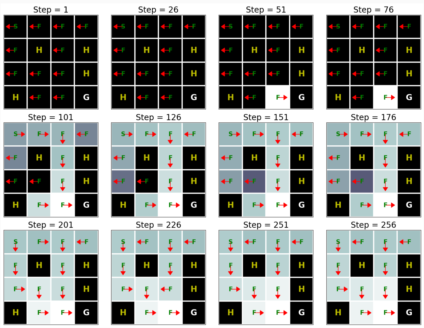
This result shows that Q-learning can find the optimal solution for this problem roughly after 250 iterations. However, when we compare this result with the Value Iteration algorithm’s result (see Implementation of Value Iteration), we can see that the Value Iteration algorithm needs way fewer iterations to find the optimal solution for this problem. This happens because the Value Iteration algorithm has access to the full MDP whereas Q-learning does not.
이 결과는 Q-learning이 대략 250번의 반복 후에 이 문제에 대한 최적의 솔루션을 찾을 수 있음을 보여줍니다. 그러나 이 결과를 Value Iteration 알고리즘의 결과(Value Iteration 구현 참조)와 비교하면 Value Iteration 알고리즘이 이 문제에 대한 최적의 솔루션을 찾기 위해 훨씬 더 적은 반복이 필요하다는 것을 알 수 있습니다. 이는 Value Iteration 알고리즘이 전체 MDP에 액세스할 수 있는 반면 Q-learning은 액세스할 수 없기 때문에 발생합니다.
17.3.6. Summary
Q-learning is one of the most fundamental reinforcement-learning algorithms. It has been at the epicenter of the recent success of reinforcement learning, most notably in learning to play video games (Mnih et al., 2013). Implementing Q-learning does not require that we know the Markov decision process (MDP), e.g., the transition and reward functions, completely.
Q-러닝은 가장 기본적인 강화학습 알고리즘 중 하나입니다. 이는 최근 강화 학습 성공의 진원지였으며, 특히 비디오 게임 학습에서 가장 두드러졌습니다(Mnih et al., 2013). Q-러닝을 구현하기 위해 MDP(Markov Decision Process)(예: 전환 및 보상 기능)를 완전히 알 필요는 없습니다.
'Dive into Deep Learning > D2L Reinforcement Learning' 카테고리의 다른 글
| D2L - 17.2. Value Iteration (0) | 2023.09.05 |
|---|---|
| D2L - 17.1. Markov Decision Process (MDP) (0) | 2023.09.05 |
| D2L-17. Reinforcement Learning (0) | 2023.09.05 |