
D2L - 18.2. Gaussian Process Priors
2023. 9. 9. 11:31 |
18.2. Gaussian Process Priors — Dive into Deep Learning 1.0.3 documentation (d2l.ai)
18.2. Gaussian Process Priors — Dive into Deep Learning 1.0.3 documentation
d2l.ai
18.2. Gaussian Process Priors
Understanding Gaussian processes (GPs) is important for reasoning about model construction and generalization, and for achieving state-of-the-art performance in a variety of applications, including active learning, and hyperparameter tuning in deep learning. GPs are everywhere, and it is in our interests to know what they are and how we can use them.
가우시안 프로세스(GP)를 이해하는 것은 모델 구성 및 일반화에 대한 추론과 능동 학습, 딥 러닝의 하이퍼파라미터 조정을 포함한 다양한 애플리케이션에서 최첨단 성능을 달성하는 데 중요합니다. GP는 어디에나 있으며, GP가 무엇인지, 어떻게 사용할 수 있는지 아는 것이 우리의 이익입니다.
In this section, we introduce Gaussian process priors over functions. In the next notebook, we show how to use these priors to do posterior inference and make predictions. The next section can be viewed as “GPs in a nutshell”, quickly giving what you need to apply Gaussian processes in practice.
이 섹션에서는 함수에 대한 Gaussian process priors를 소개를 합니다. 다음 노트북에서는 이러한 priors를 사용하여 사후 추론을 수행하고 예측하는 방법을 보여줍니다. 다음 섹션은 실제로 가우스 프로세스를 적용하는 데 필요한 내용을 빠르게 제공하는 "간단한 GP"로 볼 수 있습니다.
import numpy as np
from scipy.spatial import distance_matrix
from d2l import torch as d2l

d2l.set_figsize()
위의 코드는 Python 프로그램의 일부분이며, 주로 수학적 및 시각화 라이브러리를 사용하여 그림의 크기를 설정하는 목적으로 사용됩니다. 아래는 코드의 각 부분에 대한 설명입니다:
- import numpy as np: 이 줄은 NumPy 라이브러리를 가져오고, 'np'라는 별칭으로 라이브러리를 사용할 수 있도록 합니다. NumPy는 다차원 배열 및 행렬 연산을 위한 파이썬 라이브러리로, 수치 계산과 관련된 다양한 기능을 제공합니다.
- from scipy.spatial import distance_matrix: 이 줄은 SciPy 라이브러리에서 distance_matrix 함수를 가져옵니다. distance_matrix 함수는 점들 간의 거리 행렬을 계산하는 데 사용됩니다.
- from d2l import torch as d2l: 이 줄은 "d2l" 모듈에서 "torch" 모듈을 가져오고, "d2l" 모듈을 "d2l"로 별칭 지정합니다. 이 모듈은 D2L(Data Science for Dummies) 라이브러리의 일부로서, 딥 러닝 및 기계 학습 교육을 위한 유용한 기능과 도구를 제공합니다.
- d2l.set_figsize(): 이 줄은 D2L 라이브러리의 set_figsize 함수를 호출하여 현재 그림의 크기를 설정합니다. 이 함수는 일반적으로 그림의 크기를 조절하기 위해 사용됩니다.
이 코드 자체는 주로 라이브러리 및 설정을 가져오고 초기화하기 위한 것으로, 여기서는 실제 작업이 수행되지 않습니다. 코드의 나머지 부분이나 주변 문맥에서 더 많은 정보가 필요할 것입니다.
Gaussian Process Prior 란? (GPT 답변)
**가우시안 프로세스 사전(Gaussian Process Prior)**는 가우시안 프로세스(GP) 모델에서 사용되는 중요한 개념 중 하나입니다. GP는 확률적인 회귀 및 분류 문제를 해결하는 데 사용되는 확률적인 모델링 도구 중 하나로, 데이터 포인트 간의 관계를 모델링하는 데 사용됩니다.
가우시안 프로세스 사전은 모델링하려는 함수의 사전 정보 또는 가정을 나타냅니다. 이것은 GP 모델을 어떤 종류의 함수로 가정하고, 모델의 평균 및 공분산 구조를 결정하는 데 사용됩니다. GP 사전은 모델을 더 효과적으로 최적화하고, 모델이 데이터에 더 잘 적합하도록 도울 수 있습니다.
가우시안 프로세스 사전의 주요 요소는 다음과 같습니다:
- 평균 함수(Mean Function): GP 모델의 평균 함수는 예측 모델이 데이터를 따라 어떻게 중심에 위치해야 하는지를 제시합니다. 평균 함수는 데이터에 따라 조정될 수 있으며, 예측 모델이 평균 함수를 따라 움직입니다.
- 공분산 함수(Covariance Function 또는 Kernel 함수): GP 모델의 공분산 함수는 데이터 포인트 간의 관계를 모델링합니다. 이 함수는 데이터 포인트 간의 유사성을 측정하며, 두 데이터 포인트 사이의 거리 또는 유사성을 계산합니다. 일반적으로 RBF(Radial Basis Function) 커널, 선형 커널, 다항식 커널 등 다양한 커널 함수가 사용됩니다.
- 하이퍼파라미터(Hyperparameters): 가우시안 프로세스 사전은 평균 함수와 공분산 함수의 하이퍼파라미터를 포함합니다. 이러한 하이퍼파라미터는 GP 모델을 조정하고 데이터에 맞게 조절하는 데 사용됩니다. 하이퍼파라미터는 최적화 과정을 통해 조정됩니다.
가우시안 프로세스 사전을 설정하는 방법은 모델링하려는 문제에 따라 다르며, 경험과 도메인 지식이 필요한 경우가 많습니다. 올바른 가우시안 프로세스 사전을 선택하면 모델의 성능을 향상시키고, 데이터에 대한 불확실성을 더 정확하게 모델링할 수 있습니다.
18.2.1. Definition
A Gaussian process is defined as a collection of random variables, any finite number of which have a joint Gaussian distribution. If a function f(x) is a Gaussian process, with mean function m(x) and covariance function or kernel k(x,x′), f(x)∼GP(m,k), then any collection of function values queried at any collection of input points x (times, spatial locations, image pixels, etc.), has a joint multivariate Gaussian distribution with mean vector μ and covariance matrix K: f(x1),…,f(xn)∼N(μ,K), where μi=E[f(xi)]=m(xi) and Kij= Cov(f(xi),f(xj)) = k(xi,xj).
가우스 프로세스는 임의 변수의 모음으로 정의되며, 임의의 유한한 수는 공동 가우스 분포를 갖습니다. 함수 f(x)가 평균 함수 m(x)와 공분산 함수 또는 커널 k(x,x′), f(x)∼GP(m,k)를 갖는 가우스 프로세스인 경우 함수 값의 모음 임의의 입력 점 x(시간, 공간 위치, 이미지 픽셀 등) 모음에서 쿼리된 값은 평균 벡터 μ 및 공분산 행렬 K를 갖는 결합 다변량 가우스 분포를 갖습니다: f(x1),…,f(xn)∼N( μ,K), 여기서 μi=E[f(xi)]=m(xi)이고 Kij= Cov(f(xi),f(xj)) = k(xi,xj)입니다.
This definition may seem abstract and inaccessible, but Gaussian processes are in fact very simple objects.
이 정의는 추상적이고 접근하기 어려운 것처럼 보일 수 있지만 가우스 프로세스는 실제로 매우 간단한 개체입니다.

Any function with w drawn from a Gaussian (normal) distribution, and ϕ being any vector of basis functions, for example ϕ(x)=(1,x,x**2,...,x**d)⊤, is a Gaussian process. Moreover, any Gaussian process f(x) can be expressed in the form of equation (18.2.1). Let’s consider a few concrete examples, to begin getting acquainted with Gaussian processes, after which we can appreciate how simple and useful they really are.
가우스(정규) 분포에서 도출된 w를 갖는 모든 함수, 그리고 ф는 기본 함수의 임의의 벡터입니다. 예를 들어 'ф(x)=(1,x,x**2,...,x**d)⊤'는 가우스 프로세스입니다. 게다가 임의의 가우스 프로세스 f(x)는 방정식 (18.2.1)의 형태로 표현될 수 있습니다. 가우시안 프로세스에 익숙해지기 위해 몇 가지 구체적인 예를 고려해 보겠습니다. 그 후에는 이것이 실제로 얼마나 간단하고 유용한지 평가할 수 있습니다.
18.2.2. A Simple Gaussian Process
Suppose f(x)=w0+w1x, and w0,w1∼N(0,1), with w0,w1,x all in one dimension. We can equivalently write this function as the inner product f(x)=(w0,w1)(1,x)⊤. In (18.2.1) above, w=(w0,w1)**⊤ and ф(x)=(1,x)**⊤.
f(x)=w0+w1x, w0,w1∼N(0,1), w0,w1,x가 모두 1차원에 있다고 가정합니다. 이 함수를 내적 f(x)=(w0,w1)(1,x)⊤로 동등하게 작성할 수 있습니다. 위의 (18.2.1)에서 w=(w0,w1)**⊤ 및 ф(x)=(1,x)**⊤입니다.
For any x, f(x) is a sum of two Gaussian random variables. Since Gaussians are closed under addition, f(x) is also a Gaussian random variable for any x. In fact, we can compute for any particular x that f(x) is N(0,1+x2). Similarly, the joint distribution for any collection of function values, (f(x1),…,f(xn)), for any collection of inputs x1,…,xn, is a multivariate Gaussian distribution. Therefore f(x) is a Gaussian process.
임의의 x에 대해 f(x)는 두 가우스 확률 변수의 합입니다. 가우스는 덧셈에 대해 닫혀 있으므로 f(x)는 모든 x에 대한 가우스 확률 변수이기도 합니다. 실제로, 우리는 f(x)가 N(0,1+x2)인 특정 x에 대해 계산할 수 있습니다. 마찬가지로, 모든 입력 x1,…,xn 컬렉션에 대한 함수 값 컬렉션(f(x1),…,f(xn))에 대한 결합 분포는 다변량 가우스 분포입니다. 따라서 f(x)는 가우스 과정입니다.
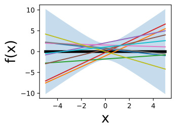
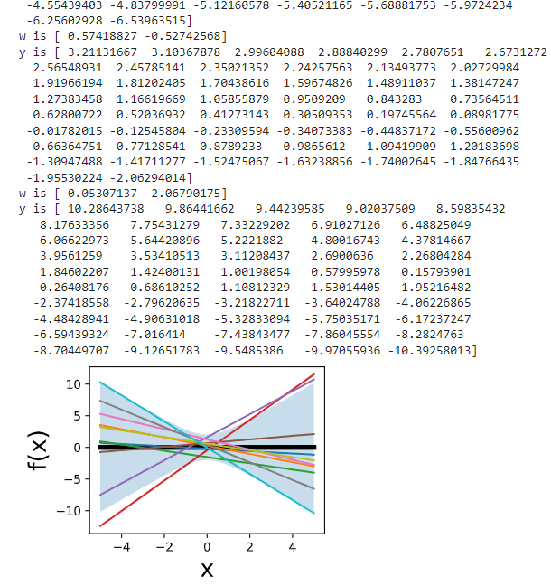
In short, f(x) is a random function, or a distribution over functions. We can gain some insights into this distribution by repeatedly sampling values for w0,w1, and visualizing the corresponding functions f(x), which are straight lines with slopes and different intercepts, as follows:
간단히 말해서, f(x)는 무작위 함수, 즉 함수에 대한 분포입니다. 다음과 같이 w0,w1에 대한 값을 반복적으로 샘플링하고 기울기와 다양한 절편이 있는 직선인 해당 함수 f(x)를 시각화하면 이 분포에 대한 통찰력을 얻을 수 있습니다.
def lin_func(x, n_sample):
    preds = np.zeros((n_sample, x.shape[0]))
    for ii in range(n_sample):
        w = np.random.normal(0, 1, 2)
        y = w[0] + w[1] * x
        preds[ii, :] = y
    return preds

x_points = np.linspace(-5, 5, 50)
outs = lin_func(x_points, 10)
lw_bd = -2 * np.sqrt((1 + x_points ** 2))
up_bd = 2 * np.sqrt((1 + x_points ** 2))

d2l.plt.fill_between(x_points, lw_bd, up_bd, alpha=0.25)
d2l.plt.plot(x_points, np.zeros(len(x_points)), linewidth=4, color='black')
d2l.plt.plot(x_points, outs.T)
d2l.plt.xlabel("x", fontsize=20)
d2l.plt.ylabel("f(x)", fontsize=20)
d2l.plt.show()
위의 코드는 주어진 선형 함수를 기반으로 데이터를 생성하고 시각화하는 파이썬 프로그램입니다. 코드의 각 부분에 대한 설명은 다음과 같습니다:
- def lin_func(x, n_sample):: 이 줄은 lin_func라는 사용자 지정 함수를 정의합니다. 이 함수는 x와 n_sample 두 개의 인자를 받습니다. x는 입력 데이터로 사용되며, n_sample은 데이터 샘플의 수를 나타냅니다.
- preds = np.zeros((n_sample, x.shape[0])): 이 줄은 결과를 저장할 빈 배열인 preds를 생성합니다. 이 배열은 n_sample개의 행과 x 배열의 길이와 같은 열을 갖습니다.
- for ii in range(n_sample):: 이 줄은 n_sample만큼 반복하는 루프를 시작합니다.
- w = np.random.normal(0, 1, 2): 이 줄은 평균이 0이고 표준편차가 1인 정규 분포에서 무작위 가중치 w를 생성합니다. w는 길이가 2인 배열로, 첫 번째 원소는 y 절편을 나타내고 두 번째 원소는 기울기를 나타냅니다.
- y = w[0] + w[1] * x: 이 줄은 입력 데이터 x에 대한 예측값 y를 계산합니다. 이 예측값은 선형 함수 w[0] + w[1] * x에 의해 생성됩니다.
- preds[ii, :] = y: 이 줄은 현재 예측값 y를 preds 배열에 저장합니다.
- return preds: 이 줄은 preds 배열을 반환하고, lin_func 함수를 종료합니다.
- x_points = np.linspace(-5, 5, 50): 이 줄은 -5부터 5까지의 범위에서 50개의 등간격으로 분포하는 x_points 배열을 생성합니다. 이 배열은 x 값의 범위를 나타냅니다.
- outs = lin_func(x_points, 10): 이 줄은 앞에서 정의한 lin_func 함수를 호출하여 x_points 값을 사용하여 예측값을 생성합니다. n_sample 매개변수로 10을 전달하므로 10개의 무작위 예측값이 생성됩니다.
- lw_bd = -2 * np.sqrt((1 + x_points ** 2)) 및 up_bd = 2 * np.sqrt((1 + x_points ** 2)): 이 두 줄은 x_points 값을 사용하여 하한(lw_bd)과 상한(up_bd) 경계를 생성합니다. 이 경계는 시각화에서 사용될 것입니다.
- d2l.plt.fill_between(x_points, lw_bd, up_bd, alpha=0.25): 이 줄은 fill_between 함수를 사용하여 x_points 범위 내에서 lw_bd와 up_bd 사이를 채우는 영역을 그립니다. alpha 매개변수는 영역의 투명도를 설정합니다.
- d2l.plt.plot(x_points, np.zeros(len(x_points)), linewidth=4, color='black'): 이 줄은 x 축에 대한 제로 라인을 그리는 것으로, 그림에서 x 축을 나타냅니다.
- d2l.plt.plot(x_points, outs.T): 이 줄은 outs 배열을 사용하여 x 축에 대한 예측값을 그립니다. 여러 개의 예측값이 그려질 것이며, 각 예측값은 서로 다른 색상으로 표시됩니다.
- d2l.plt.xlabel("x", fontsize=20) 및 d2l.plt.ylabel("f(x)", fontsize=20): 이 두 줄은 x 축과 y 축에 라벨을 추가하고 글꼴 크기를 설정합니다.
- d2l.plt.show(): 이 줄은 그림을 화면에 표시합니다.
이 코드는 주어진 선형 함수에 기반하여 데이터를 생성하고 시각적으로 나타내는 데 사용됩니다. 결과 그림에는 선형 함수를 따라 생성된 데이터 포인트와 해당 경계가 표시됩니다.

If w0 and w1 are instead drawn from N(0,a2), how do you imagine varying 'a' affects the distribution over functions?
w0과 w1이 N(0,a2)에서 대신 추출된다면 'a'의 변화가 함수 분포에 어떤 영향을 미칠 것이라고 생각하시나요?
18.2.3. From Weight Space to Function Space
In the plot above, we saw how a distribution over parameters in a model induces a distribution over functions. While we often have ideas about the functions we want to model — whether they’re smooth, periodic, quickly varying, etc. — it is relatively tedious to reason about the parameters, which are largely uninterpretable. Fortunately, Gaussian processes provide an easy mechanism to reason directly about functions. Since a Gaussian distribution is entirely defined by its first two moments, its mean and covariance matrix, a Gaussian process by extension is defined by its mean function and covariance function.
위의 플롯에서 모델의 매개변수에 대한 분포가 함수에 대한 분포를 유도하는 방법을 확인했습니다. 우리는 모델링하려는 함수에 대한 아이디어(매끄럽거나 주기적이거나 빠르게 변화하는 등)에 대해 종종 아이디어를 갖고 있지만 대체로 해석할 수 없는 매개변수에 대해 추론하는 것은 상대적으로 지루합니다. 다행스럽게도 가우스 프로세스는 함수에 대해 직접적으로 추론할 수 있는 쉬운 메커니즘을 제공합니다. 가우스 분포는 처음 두 모멘트인 평균과 공분산 행렬로 완전히 정의되므로 확장에 따른 가우스 프로세스는 평균 함수와 공분산 함수로 정의됩니다.
In the above example, the mean function 위의 예에서 평균 함수는

Similarly, the covariance function is 마찬가지로 공분산 함수는 다음과 같습니다.

Our distribution over functions can now be directly specified and sampled from, without needing to sample from the distribution over parameters. For example, to draw from f(x), we can simply form our multivariate Gaussian distribution associated with any collection of x we want to query, and sample from it directly. We will begin to see just how advantageous this formulation will be.
이제 매개변수에 대한 분포에서 샘플링할 필요 없이 함수에 대한 분포를 직접 지정하고 샘플링할 수 있습니다. 예를 들어 f(x)에서 추출하려면 쿼리하려는 x 컬렉션과 관련된 다변량 가우스 분포를 간단히 구성하고 여기에서 직접 샘플링하면 됩니다. 우리는 이 공식이 얼마나 유리한지 살펴보기 시작할 것입니다.
First, we note that essentially the same derivation for the simple straight line model above can be applied to find the mean and covariance function for any model of the form f(x)=w**⊤ ϕ(x), with w∼N(u,S). In this case, the mean function m(x)=u**⊤ ϕ(x), and the covariance function k(x,x′)=ϕ(x)**⊤ Sϕ(x′). Since ϕ(x) can represent a vector of any non-linear basis functions, we are considering a very general model class, including models with an even an infinite number of parameters.
먼저, 위의 단순 직선 모델에 대해 본질적으로 동일한 파생을 적용하여 'w∼N(u,S)와 함께 f(x)=w**⊤ ф(x) 형식의 모든 모델에 대한 평균 및 공분산 함수를 찾을 수 있습니다.. 이 경우 평균 함수 m(x)=u**⊤ ф(x)이고, 공분산 함수 k(x,x′)=ψ(x)**⊤ Sψ(x′)입니다. ф(x)는 모든 비선형 기저 함수의 벡터를 나타낼 수 있으므로 우리는 무한한 수의 매개변수를 가진 모델을 포함하여 매우 일반적인 모델 클래스를 고려하고 있습니다.
18.2.4. The Radial Basis Function (RBF) Kernel
The radial basis function (RBF) kernel is the most popular covariance function for Gaussian processes, and kernel machines in general. This kernel has the form kRBF(x,x′)=a**2 exp(−1/2ℓ**2||x−x′||2), where 'a' is an amplitude parameter, and ℓ is a lengthscale hyperparameter.
RBF(방사형 기저 함수) 커널은 가우스 프로세스 및 일반적으로 커널 머신에 가장 널리 사용되는 공분산 함수입니다. 이 커널은 kRBF(x,x′)=a**2 exp(−1/2ℓ**2||x−x′||2) 형식을 갖습니다. 여기서 'a'는 진폭 매개변수이고 ℓ는 길이 척도 하이퍼 매개변수입니다.
Radial Basis Function (RBF) Kernel 이란? (GPT3.5 의 답변)
The Radial Basis Function (RBF) kernel, also known as the Gaussian kernel, is a commonly used kernel function in machine learning and statistical modeling. It is particularly popular in the context of Support Vector Machines (SVMs) and Gaussian Processes (GPs).
라디얼 베이시스 함수(Radial Basis Function, RBF) 커널은 기계 학습 및 통계 모델링에서 일반적으로 사용되는 커널 함수로, 특히 서포트 벡터 머신(SVM)과 가우시안 프로세스(GP)의 맥락에서 널리 사용됩니다.
The RBF kernel is defined as: RBF 커널은 다음과 같이 정의됩니다.
K(x, x') = exp(-γ * ||x - x'||^2)
Here, K represents the kernel function, x and x' are data points, ||x - x'|| represents the Euclidean distance between these points, and γ (gamma) is a hyperparameter that controls the kernel's shape. The RBF kernel assigns a similarity or correlation score to pairs of data points based on their distance.
여기서 K는 커널 함수를 나타내며, x와 x'은 데이터 포인트이고, ||x - x'||은 이러한 포인트 간의 유클리드 거리를 나타내며, γ(gamma)는 커널의 모양을 제어하는 하이퍼파라미터입니다. RBF 커널은 데이터 포인트 쌍에 대해 거리를 기반으로 유사성 또는 상관 점수를 할당합니다.
Key characteristics of the RBF kernel include:
RBF 커널의 주요 특징은 다음과 같습니다.
- Decay with Distance: As the distance between data points increases, the similarity score assigned by the RBF kernel decreases exponentially. This means that nearby points receive higher similarity scores, while distant points receive lower scores.
거리에 따른 감쇠: 데이터 포인트 간 거리가 증가함에 따라 RBF 커널이 할당하는 유사성 점수가 지수적으로 감소합니다. 이것은 가까운 포인트가 더 높은 유사성 점수를 받는 반면 먼 포인트가 더 낮은 점수를 받는다는 것을 의미합니다. - Smoothness: The RBF kernel produces smooth and continuous similarity scores, which makes it suitable for capturing complex patterns and relationships in the data.
부드러움: RBF 커널은 부드럽고 연속적인 유사성 점수를 생성하며, 이로써 데이터의 복잡한 패턴과 관계를 캡처하는 데 적합합니다. - Universal Approximator: The RBF kernel is a universal approximator, meaning it can approximate any continuous function with sufficient data and proper tuning of its hyperparameters.
범용 근사자(Universal Approximator): RBF 커널은 범용 근사자로, 충분한 데이터와 하이퍼파라미터의 적절한 조정을 통해 어떤 연속 함수든 근사화할 수 있습니다. - Hyperparameter γ: The hyperparameter γ controls the "width" of the kernel. Smaller values of γ result in a broader kernel that assigns higher similarity scores to a wider range of data points. Larger values of γ result in a narrower kernel that focuses on closer neighbors.
하이퍼파라미터 γ: 하이퍼파라미터 γ는 커널의 "폭"을 제어합니다. 작은 γ 값은 더 넓은 커널을 생성하여 더 넓은 범위의 데이터 포인트에 높은 유사성 점수를 할당합니다. 큰 γ 값은 더 좁은 커널을 생성하여 더 가까운 이웃에 중점을 둡니다.
The RBF kernel is often used in various machine learning tasks, such as SVM classification, GP regression, clustering, and dimensionality reduction. It is valued for its ability to capture complex, non-linear relationships in the data, but it may also be sensitive to the choice of the γ hyperparameter, which requires careful tuning for optimal model performance.
RBF 커널은 SVM 분류, GP 회귀, 클러스터링 및 차원 축소와 같은 다양한 기계 학습 작업에서 사용됩니다. 이는 데이터의 복잡한 비선형 관계를 캡처할 수 있는 능력으로 인해 중요하며, 최적의 모델 성능을 위해 γ 하이퍼파라미터 선택에 주의 깊게 조정해야 할 수도 있습니다.
Let’s derive this kernel starting from weight space. Consider the function
가중치 공간에서 시작하여 이 커널을 유도해 보겠습니다. 기능을 고려하십시오

f(x) is a sum of radial basis functions, with width ℓ, centred at the points ci, as shown in the following figure.
f(x)는 다음 그림과 같이 점 ci를 중심으로 너비가 ℓ인 방사형 기저 함수의 합입니다.
We can recognize f(x) as having the form w**⊤ ϕ(x), where w=(w1,…,wJ)**⊤ and ϕ(x) is a vector containing each of the radial basis functions. The covariance function of this Gaussian process is then
f(x)는 w**⊤ ф(x) 형식을 갖는 것으로 인식할 수 있습니다. 여기서 w=(w1,…,wJ)**⊤이고 ф(x)는 각 방사형 기저 함수를 포함하는 벡터입니다. 이 가우스 프로세스의 공분산 함수는 다음과 같습니다.

Now let’s consider what happens as we take the number of parameters (and basis functions) to infinity. Let cJ=logJ, c1=−log J, and ci+1−ci=Δc=2 logJ/J, and J→∞. The covariance function becomes the Riemann sum:
이제 매개변수(및 기본 함수)의 수를 무한대로 가져가면 어떤 일이 발생하는지 생각해 보겠습니다. cJ=logJ, c1=−log J, 그리고 ci+1−ci=Δc=2 logJ/J, 그리고 J→라고 하자. 공분산 함수는 리만 합계가 됩니다.

By setting c0=−∞ and c∞=∞, we spread the infinitely many basis functions across the whole real line, each a distance Δc→0 apart:
c0=−무한대와 c무한대=무를 설정함으로써 우리는 무한히 많은 기저 함수를 실제 선 전체에 걸쳐 각각 Δc→0 거리만큼 분산시킵니다.

It is worth taking a moment to absorb what we have done here. By moving into the function space representation, we have derived how to represent a model with an infinite number of parameters, using a finite amount of computation. A Gaussian process with an RBF kernel is a universal approximator, capable of representing any continuous function to arbitrary precision. We can intuitively see why from the above derivation. We can collapse each radial basis function to a point mass taking ℓ→0, and give each point mass any height we wish.
여기서 우리가 한 일을 잠시 흡수해 볼 가치가 있습니다. 함수 공간 표현으로 이동하여 유한한 양의 계산을 사용하여 무한한 수의 매개변수가 있는 모델을 표현하는 방법을 도출했습니다. RBF 커널을 사용하는 가우스 프로세스는 모든 연속 함수를 임의의 정밀도로 표현할 수 있는 범용 근사기입니다. 위의 도출을 통해 그 이유를 직관적으로 알 수 있습니다. 각 방사형 기저 함수를 ℓ→0을 취하는 점 질량으로 축소하고 각 점 질량에 원하는 높이를 부여할 수 있습니다.
So a Gaussian process with an RBF kernel is a model with an infinite number of parameters and much more flexibility than any finite neural network. Perhaps all the fuss about overparametrized neural networks is misplaced. As we will see, GPs with RBF kernels do not overfit, and in fact provide especially compelling generalization performance on small datasets. Moreover, the examples in (Zhang et al., 2021), such as the ability to fit images with random labels perfectly, but still generalize well on structured problems, (can be perfectly reproduced using Gaussian processes) (Wilson and Izmailov, 2020). Neural networks are not as distinct as we make them out to be.
따라서 RBF 커널을 사용하는 가우스 프로세스는 무한한 수의 매개 변수와 유한 신경망보다 훨씬 더 많은 유연성을 갖춘 모델입니다. 아마도 과도하게 매개변수화된 신경망에 대한 모든 소란은 잘못된 것일 수도 있습니다. 앞으로 살펴보겠지만 RBF 커널을 사용하는 GP는 과적합되지 않으며 실제로 작은 데이터 세트에서 특히 강력한 일반화 성능을 제공합니다. 더욱이 (Zhang et al., 2021)의 예에서는 임의의 레이블이 있는 이미지를 완벽하게 맞추면서도 구조화된 문제에 대해 여전히 잘 일반화하는 기능과 같은 것입니다(가우시안 프로세스를 사용하여 완벽하게 재현 가능)(Wilson and Izmailov, 2020). . 신경망은 우리가 생각하는 것만큼 뚜렷하지 않습니다.
We can build further intuition about Gaussian processes with RBF kernels, and hyperparameters such as length-scale, by sampling directly from the distribution over functions. As before, this involves a simple procedure:
함수에 대한 분포에서 직접 샘플링함으로써 RBF 커널과 길이 척도와 같은 하이퍼파라미터를 사용하는 가우스 프로세스에 대한 추가 직관을 구축할 수 있습니다. 이전과 마찬가지로 여기에는 간단한 절차가 포함됩니다.
- Choose the input x points we want to query the GP: x1,…,xn.
GP에 쿼리하려는 입력 x 포인트(x1,…,xn)를 선택합니다. - Evaluate m(xi), i=1,…,n, and k(xi,xj) for i,j=1,…,n to respectively form the mean vector and covariance matrix μ and K, where (f(x1),…,f(xn))∼N(μ,K).
i,j=1,…,n에 대해 m(xi), i=1,…,n 및 k(xi,xj)를 계산하여 각각 평균 벡터와 공분산 행렬 μ 및 K를 형성합니다. 여기서 (f(x1) ,…,f(xn))∼N(μ,K). - Sample from this multivariate Gaussian distribution to obtain the sample function values.
이 다변량 가우스 분포에서 샘플링하여 샘플 함수 값을 얻습니다. - Sample more times to visualize more sample functions queried at those points.
더 많은 횟수를 샘플링하여 해당 지점에서 쿼리된 더 많은 샘플 함수를 시각화합니다.
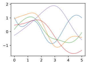
We illustrate this process in the figure below.
아래 그림에서는 이 프로세스를 설명합니다.
def rbfkernel(x1, x2, ls=4.):  #@save
    dist = distance_matrix(np.expand_dims(x1, 1), np.expand_dims(x2, 1))
    return np.exp(-(1. / ls / 2) * (dist ** 2))

x_points = np.linspace(0, 5, 50)
meanvec = np.zeros(len(x_points))
covmat = rbfkernel(x_points,x_points, 1)

prior_samples= np.random.multivariate_normal(meanvec, covmat, size=5);
d2l.plt.plot(x_points, prior_samples.T, alpha=0.5)
d2l.plt.show()
위의 코드는 라디언 기저 함수(Radial Basis Function, RBF) 커널을 사용하여 가우시안 프로세스(Gaussian Process)의 사전 분포를 시각화하는 파이썬 프로그램입니다. 이 코드를 한 줄씩 설명하겠습니다:
- def rbfkernel(x1, x2, ls=4.):: 이 줄은 rbfkernel 함수를 정의합니다. 이 함수는 두 개의 입력 x1과 x2를 받고, 추가적인 매개변수로 ls를 받습니다. ls는 커널의 길이 스케일을 나타내는 매개변수로, 기본값은 4입니다.
- dist = distance_matrix(np.expand_dims(x1, 1), np.expand_dims(x2, 1)): 이 줄은 입력 데이터 x1과 x2 사이의 거리 행렬(dist)을 계산합니다. distance_matrix 함수를 사용하여 x1과 x2 간의 모든 가능한 거리를 계산합니다.
- return np.exp(-(1. / ls / 2) * (dist ** 2)): 이 줄은 RBF 커널의 계산을 수행합니다. RBF 커널은 가우시안 형태로, 두 데이터 포인트 간의 거리를 지수 함수의 형태로 변환하여 반환합니다. ls는 커널의 길이 스케일을 조절하는 매개변수로, 커널의 폭을 조절합니다.
- x_points = np.linspace(0, 5, 50): 이 줄은 0부터 5까지의 범위에서 50개의 등간격으로 분포하는 x_points 배열을 생성합니다. 이 배열은 x 값의 범위를 나타냅니다.
- meanvec = np.zeros(len(x_points)): 이 줄은 x_points와 같은 길이의 제로 벡터인 meanvec를 생성합니다. 이 벡터는 가우시안 프로세스의 평균 벡터로 사용됩니다.
- covmat = rbfkernel(x_points, x_points, 1): 이 줄은 rbfkernel 함수를 호출하여 x_points에 대한 공분산 행렬(covmat)을 계산합니다. 이 공분산 행렬은 RBF 커널을 사용하여 생성되며, ls 매개변수의 값이 1로 설정되어 있습니다.
- prior_samples = np.random.multivariate_normal(meanvec, covmat, size=5): 이 줄은 meanvec와 covmat을 사용하여 가우시안 분포에서 5개의 무작위 샘플(prior_samples)을 생성합니다. 이 샘플은 가우시안 프로세스의 사전 분포에서 추출된 것입니다.
- d2l.plt.plot(x_points, prior_samples.T, alpha=0.5): 이 줄은 prior_samples를 시각화합니다. 각각의 무작위 샘플은 x_points에 대해 그래프로 표시되며, alpha 매개변수를 사용하여 투명도를 설정합니다.
- d2l.plt.show(): 이 줄은 그래프를 화면에 표시합니다.
이 코드는 가우시안 프로세스의 사전 분포를 시각화하기 위해 RBF 커널을 사용하는 간단한 예제를 제공합니다. 이를 통해 가우시안 프로세스가 어떻게 작동하는지 이해할 수 있습니다.

18.2.5. The Neural Network Kernel
Research on Gaussian processes in machine learning was triggered by research on neural networks. Radford Neal was pursuing ever larger Bayesian neural networks, ultimately showing in 1994 (later published in 1996, as it was one of the most infamous NeurIPS rejections) that such networks with an infinite number of hidden units become Gaussian processes with particular kernel functions (Neal, 1996). Interest in this derivation has re-surfaced, with ideas like the neural tangent kernel being used to investigate the generalization properties of neural networks (Matthews et al., 2018) (Novak et al., 2018). We can derive the neural network kernel as follows.
기계 학습의 가우스 프로세스에 대한 연구는 신경망에 대한 연구에서 시작되었습니다. Radford Neal은 훨씬 더 큰 베이지안 신경망을 추구했으며, 궁극적으로 1994년에(나중에 가장 악명 높은 NeurIPS 거부 중 하나인 1996년에 출판됨) 무한한 수의 숨겨진 단위를 가진 그러한 네트워크가 특정 커널 기능을 가진 가우스 프로세스가 된다는 것을 보여주었습니다(Neal , 1996). 신경망의 일반화 속성을 조사하는 데 신경 접선 커널과 같은 아이디어가 사용되면서 이 파생에 대한 관심이 다시 표면화되었습니다(Matthews et al., 2018)(Novak et al., 2018). 신경망 커널은 다음과 같이 유도할 수 있습니다.
Consider a neural network function f(x) with one hidden layer:
하나의 은닉층이 있는 신경망 함수 f(x)를 생각해 보세요.
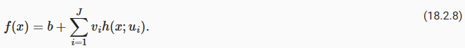
b is a bias, vi are the hidden to output weights, ℎ is any bounded hidden unit transfer function, ui are the input to hidden weights, and J is the number of hidden units. Let b and vi be independent with zero mean and variances σ**2 b and σ**2v/J, respectively, and let the ui have independent identical distributions. We can then use the central limit theorem to show that any collection of function values f(x1),…,f(xn) has a joint multivariate Gaussian distribution.
b는 편향, vi는 출력 가중치에 대한 은닉, ℎ는 경계가 있는 숨겨진 단위 전달 함수, ui는 숨겨진 가중치에 대한 입력, J는 숨겨진 단위의 수입니다. b와 vi가 평균이 0이고 분산이 각각 σ**2 b 및 σ**2v/J인 독립이고 ui가 독립적인 동일한 분포를 갖는다고 가정합니다. 그런 다음 중심 극한 정리를 사용하여 함수 값 f(x1),…,f(xn)의 집합이 결합 다변량 가우스 분포를 가짐을 보여줄 수 있습니다.
The mean and covariance function of the corresponding Gaussian process are:
해당 가우스 프로세스의 평균 및 공분산 함수는 다음과 같습니다.
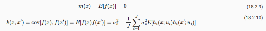
In some cases, we can essentially evaluate this covariance function in closed form. Let ℎ(x;u)=erf(u0+∑**p j=1 ujxj), where

The RBF kernel is stationary, meaning that it is translation invariant, and therefore can be written as a function of T=x−x′. Intuitively, stationarity means that the high-level properties of the function, such as rate of variation, do not change as we move in input space. The neural network kernel, however, is non-stationary. Below, we show sample functions from a Gaussian process with this kernel. We can see that the function looks qualitatively different near the origin.
RBF 커널은 고정적입니다. 즉, 변환 불변이므로 T=x−x′의 함수로 작성할 수 있습니다. 직관적으로 정상성은 입력 공간에서 이동할 때 변동률과 같은 함수의 상위 수준 속성이 변경되지 않음을 의미합니다. 그러나 신경망 커널은 고정되어 있지 않습니다. 아래에서는 이 커널을 사용한 가우스 프로세스의 샘플 함수를 보여줍니다. 함수가 원점 근처에서 질적으로 다르게 보이는 것을 볼 수 있습니다.
18.2.6. Summary
The first step in performing Bayesian inference involves specifying a prior. Gaussian processes can be used to specify a whole prior over functions. Starting from a traditional “weight space” view of modelling, we can induce a prior over functions by starting with the functional form of a model, and introducing a distribution over its parameters. We can alternatively specify a prior distribution directly in function space, with properties controlled by a kernel. The function-space approach has many advantages. We can build models that actually correspond to an infinite number of parameters, but use a finite amount of computation! Moreover, while these models have a great amount of flexibility, they also make strong assumptions about what types of functions are a priori likely, leading to relatively good generalization on small datasets.
베이지안 추론을 수행하는 첫 번째 단계는 사전 지정을 포함합니다. 가우스 프로세스를 사용하여 함수보다 전체 prior 을 지정할 수 있습니다. 모델링의 전통적인 "가중치 공간" 관점에서 시작하여 모델의 기능적 형태로 시작하고 해당 매개변수에 대한 분포를 도입함으로써 기능에 대한 사전 예측을 유도할 수 있습니다. 또는 커널에 의해 제어되는 속성을 사용하여 함수 공간에서 직접 사전 분포를 지정할 수도 있습니다. 기능 공간 접근 방식에는 많은 장점이 있습니다. 실제로 무한한 수의 매개변수에 해당하는 모델을 구축할 수 있지만 계산량은 한정되어 있습니다. 더욱이 이러한 모델은 상당한 유연성을 갖고 있지만 어떤 유형의 함수가 선험적으로 발생할 가능성이 있는지에 대한 강력한 가정을 만들어 소규모 데이터 세트에 대해 상대적으로 좋은 일반화를 이끌어냅니다.
The assumptions of models in function space are intuitively controlled by kernels, which often encode higher level properties of functions, such as smoothness and periodicity. Many kernels are stationary, meaning that they are translation invariant. Functions drawn from a Gaussian process with a stationary kernel have roughly the same high-level properties (such as rate of variation) regardless of where we look in the input space.
함수 공간에서 모델의 가정은 커널에 의해 직관적으로 제어되며, 커널은 부드러움 및 주기성과 같은 함수의 더 높은 수준 속성을 인코딩하는 경우가 많습니다. 많은 커널은 고정되어 있습니다. 즉, 변환 불변성을 의미합니다. 고정 커널을 사용하는 가우스 프로세스에서 도출된 함수는 입력 공간에서 보는 위치에 관계없이 대략 동일한 높은 수준의 속성(예: 변동률)을 갖습니다.
Gaussian processes are a relatively general model class, containing many examples of models we are already familiar with, including polynomials, Fourier series, and so on, as long as we have a Gaussian prior over the parameters. They also include neural networks with an infinite number of parameters, even without Gaussian distributions over the parameters. This connection, discovered by Radford Neal, triggered machine learning researchers to move away from neural networks, and towards Gaussian processes.
가우스 프로세스는 매개변수에 대한 가우스 사전이 있는 한 다항식, 푸리에 급수 등을 포함하여 우리에게 이미 익숙한 모델의 많은 예를 포함하는 비교적 일반적인 모델 클래스입니다. 또한 매개변수에 대한 가우스 분포가 없더라도 매개변수 수가 무한한 신경망도 포함됩니다. Radford Neal이 발견한 이 연결은 기계 학습 연구자들이 신경망에서 벗어나 가우스 프로세스로 이동하도록 촉발했습니다.
18.2.7. Exercises

'Dive into Deep Learning > D2L Gaussian Processes' 카테고리의 다른 글
| D2L - 18.3. Gaussian Process Inference (0) | 2023.09.10 |
|---|---|
| D2L - 18.1. Introduction to Gaussian Processes (0) | 2023.09.09 |
| D2L - 18. Gaussian Processes (0) | 2023.09.09 |