

https://d2l.ai/chapter_attention-mechanisms-and-transformers/vision-transformer.html
11.8. Transformers for Vision — Dive into Deep Learning 1.0.0-beta0 documentation
d2l.ai
The Transformer architecture was initially proposed for sequence to sequence learning, with a focus on machine translation. Subsequently, Transformers emerged as the model of choice in various natural language processing tasks (Brown et al., 2020, Devlin et al., 2018, Radford et al., 2018, Radford et al., 2019, Raffel et al., 2020). However, in the field of computer vision the dominant architecture has remained the CNN (Section 8). Naturally, researchers started to wonder if it might be possible to do better by adapting Transformer models to image data. This question sparked immense interest in the computer vision community. Recently, Ramachandran et al. (2019) proposed a scheme for replacing convolution with self-attention. However, its use of specialized patterns in attention makes it hard to scale up models on hardware accelerators. Then, Cordonnier et al. (2020) theoretically proved that self-attention can learn to behave similarly to convolution. Empirically, 2×2 patches were taken from images as inputs, but the small patch size makes the model only applicable to image data with low resolutions.
Transformer 아키텍처는 처음에 기계 번역에 중점을 둔 sequence to sequence learning을 위해 제안되었습니다. 이후 Transformers는 다양한 자연어 처리 작업에서 선택 모델로 등장했습니다(Brown et al., 2020, Devlin et al., 2018, Radford et al., 2018, Radford et al., 2019, Raffel et al., 2020). ). 그러나 컴퓨터 비전 분야에서 지배적인 아키텍처는 CNN으로 남아 있습니다(섹션 8). 당연히 연구자들은 Transformer 모델을 이미지 데이터에 적용하여 더 잘할 수 있을지 궁금해하기 시작했습니다. 이 질문은 컴퓨터 비전 커뮤니티에서 엄청난 관심을 불러일으켰습니다. 최근 Ramachandran et al. (2019)는 컨볼루션을 self-attention으로 대체하는 방식을 제안했습니다. 그러나 어텐션에 특화된 패턴을 사용하면 hardware accelerators에서 모델을 확장하기가 어렵습니다. ??? 그런 다음 Cordonnier et al. (2020)은 self-attention이 convolution과 유사하게 동작하도록 학습할 수 있음을 이론적으로 증명했습니다. 경험적으로 이미지에서 2×2 패치를 입력으로 가져왔지만 패치 크기가 작기 때문에 모델은 해상도가 낮은 이미지 데이터에만 적용할 수 있습니다.
Without specific constraints on patch size, vision Transformers (ViTs) extract patches from images and feed them into a Transformer encoder to obtain a global representation, which will finally be transformed for classification (Dosovitskiy et al., 2021). Notably, Transformers show better scalability than CNNs: when training larger models on larger datasets, vision Transformers outperform ResNets by a significant margin. Similar to the landscape of network architecture design in natural language processing, Transformers also became a game-changer in computer vision.
패치 크기에 대한 특정 제약 없이 vision Transformers (ViTs)는 이미지에서 패치를 추출하고 트랜스포머 인코더에 공급하여 최종적으로 분류를 위해 변환될 글로벌 representation을 얻습니다(Dosovitskiy et al., 2021). 특히 트랜스포머는 CNN보다 더 나은 확장성을 보여줍니다. 더 큰 데이터 세트에서 더 큰 모델을 교육할 때 비전 트랜스포머는 ResNets보다 훨씬 뛰어난 성능을 보입니다. 자연어 처리의 네트워크 아키텍처 설계 환경과 유사하게 Transformers도 컴퓨터 비전의 게임 체인저가 되었습니다.
import torch
from torch import nn
from d2l import torch as d2l
11.8.1. Model
Fig. 11.8.1 depicts the model architecture of vision Transformers. This architecture consists of a stem that patchifies images, a body based on the multi-layer Transformer encoder, and a head that transforms the global representation into the output label.
그림 11.8.1은 비전 트랜스포머의 모델 아키텍처를 보여줍니다. 이 아키텍처는 이미지를 패치하는 stem , multi-layer Transformer encoder를 기반으로 하는 body, global representation을 output label로 변환하는 head 로 구성됩니다.
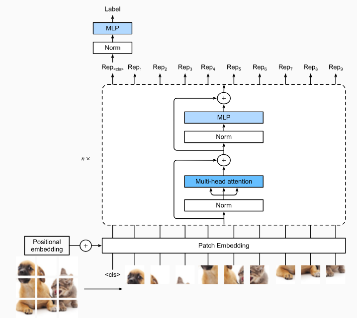
Consider an input image with height ℎ, width h, and w channels. Specifying the patch height and width both as p, the image is split into a sequence of m=ℎw/p^2 patches, where each patch is flattened to a vector of length cp^2. In this way, image patches can be treated similarly to tokens in text sequences by Transformer encoders. A special “<cls>” (class) token and the m flattened image patches are linearly projected into a sequence of m+1 vectors, summed with learnable positional embeddings. The multi-layer Transformer encoder transforms m+1 input vectors into the same amount of output vector representations of the same length. It works exactly the same way as the original Transformer encoder in Fig. 11.7.1, only differing in the position of normalization. Since the “<cls>” token attends to all the image patches via self-attention (see Fig. 11.6.1), its representation from the Transformer encoder output will be further transformed into the output label.
높이 ℎ, 너비 h 및 w 채널이 있는 입력 이미지를 고려하십시오. 패치 높이와 너비를 모두 p로 지정하면 이미지가 m=ℎw/p^2 패치 시퀀스로 분할되며 각 패치는 길이 cp^2의 벡터로 병합됩니다. 이러한 방식으로 이미지 패치는 Transformer 인코더에 의해 텍스트 시퀀스의 토큰과 유사하게 처리될 수 있습니다. 특수 "<cls>"(클래스) 토큰과 m개의 평면화된 이미지 패치는 학습 가능한 위치 임베딩으로 합산된 일련의 m+1 벡터로 선형 투영됩니다. 다층 트랜스포머 인코더는 m+1개의 입력 벡터를 같은 길이의 같은 양의 출력 벡터 표현representations 으로 변환합니다. 정규화 위치만 다를 뿐 그림 11.7.1의 원래 Transformer 인코더와 정확히 동일한 방식으로 작동합니다. "<cls>" 토큰은 self-attention(그림 11.6.1 참조)을 통해 모든 이미지 패치에 attends 하므로 Transformer 인코더 출력의 representation 은 출력 레이블로 추가 변환됩니다.
Tip. Deep Learning에서 Feature와 Representation 이란?
In the context of deep learning, the terms "feature" and "representation" are closely related concepts, but they have slightly different meanings.
딥 러닝의 맥락에서 "특징"과 "표현"이라는 용어는 밀접한 관련이 있는 개념이지만, 약간의 차이가 있습니다.
Feature: A feature refers to a specific property, characteristic, or aspect of the input data that is relevant for solving a particular task. Features are often extracted or selected from raw data to provide meaningful and informative input to a machine learning or deep learning model. Features can be thought of as the input variables or attributes that the model uses to make predictions or decisions. In deep learning, features can be learned automatically through the layers of a neural network.
특징은 특정 작업을 해결하는 데 관련성 있는 입력 데이터의 특정 속성, 특성 또는 측면을 나타냅니다. 특징은 종종 원시 데이터에서 추출되거나 선택되어 기계 학습 또는 딥 러닝 모델에 의해 의미 있는 정보를 제공하는 입력을 제공합니다. 특징은 모델이 예측하거나 결정하는 데 사용하는 입력 변수 또는 속성으로 생각할 수 있습니다. 딥 러닝에서는 특징은 신경망의 레이어를 통해 자동으로 학습될 수 있습니다.
For example, in image recognition, features could be the presence of edges, corners, textures, or specific patterns within an image. In natural language processing, features could include the frequency of certain words or phrases in a text document.
예를 들어 이미지 인식에서 특징은 이미지 내의 가장자리, 모서리, 질감 또는 특정 패턴의 존재와 관련이 있을 수 있습니다. 자연어 처리에서 특징은 텍스트 문서에서 특정 단어 또는 구문의 빈도와 관련할 수 있습니다.
Representation: Representation, on the other hand, is a broader term that encompasses the entire encoding of the input data in a format that can be processed by a machine learning model. Representation refers to how the input data is transformed and structured to be compatible with the model's architecture and learning process. It includes both the extracted features and any additional transformation that might be applied to the data.
한편, 표현은 입력 데이터를 모델이 처리할 수 있는 형식으로 전체적으로 인코딩하는 것을 나타냅니다. 표현은 입력 데이터가 모델의 아키텍처 및 학습 과정과 호환되도록 변환되고 구조화된 방식을 포함합니다. 이것은 추출된 특징 및 데이터에 적용된 추가 변환을 모두 포함합니다.
In deep learning, representations are often learned hierarchically through the layers of neural networks. Each layer extracts increasingly abstract and complex features from the previous layer's representation, gradually building a more informative and discriminating representation of the input data. The final learned representation is then used for making predictions or classifications.
딥 러닝에서 표현은 종종 신경망의 레이어를 통해 계층적으로 학습됩니다. 각 레이어는 이전 레이어의 표현에서 점점 추상적이고 복잡한 특징을 추출하여 입력 데이터의 보다 의미 있는 표현을 점진적으로 구축합니다. 최종 학습된 표현은 예측이나 분류를 위해 사용됩니다.
In summary, features are specific characteristics of the data that are relevant to a task, while representation is the overall encoding of the data that captures relevant information and is used by the model for learning and making predictions.
요약하자면, 특징은 작업에 관련된 데이터의 특정 특성이며, 표현은 입력 데이터의 전체적인 인코딩으로써 관련 정보를 포착하고 모델의 학습과 예측에 사용되는 것입니다.
CNN에서 Channel 이란?
In Convolutional Neural Networks (CNNs), a "channel" refers to one of the dimensions of the input data and the corresponding learned filters. In the context of images, which are commonly used with CNNs, the term "channel" typically refers to the color channels or color planes of an image. Each channel represents a specific color component: red, green, and blue (RGB), in the case of a standard color image.
합성곱 신경망(CNN)에서 "채널"은 입력 데이터와 해당하는 학습된 필터의 차원 중 하나를 가리킵니다. 이미지와 함께 주로 사용되는 CNN의 맥락에서 "채널"이라는 용어는 일반적으로 이미지의 색상 채널 또는 컬러 플레인을 의미합니다. 각 채널은 특정한 색상 구성요소를 나타냅니다. 표준 컬러 이미지의 경우 빨강, 초록 및 파랑(RGB)에 해당하는 채널이 있습니다.
For example, in an RGB image, there are three color channels: one for red, one for green, and one for blue. Each channel contains pixel values that represent the intensity of the corresponding color component for each pixel in the image. These channels are stacked together to create the full color image.
예를 들어 RGB 이미지에서는 세 가지 색상 채널이 있습니다: 빨강, 초록, 파랑 각각에 하나씩입니다. 각 채널에는 이미지의 각 픽셀에 대한 해당 색상 구성요소의 강도를 나타내는 픽셀 값이 포함되어 있습니다. 이러한 채널은 함께 쌓여 전체 컬러 이미지를 생성합니다.
When a CNN processes an image, it performs convolution operations on each channel separately. The learned filters, also known as kernels, are applied to each channel to extract various features. The convolutional layers in a CNN are responsible for learning these filters and combining the information from different channels to detect patterns, textures, and structures in the input image.
CNN이 이미지를 처리할 때 각 채널별로 합성곱 연산을 수행합니다. 학습된 필터 또는 커널이 각 채널에 적용되어 입력 이미지의 다양한 특징을 추출합니다. CNN의 합성곱 레이어는 이러한 필터를 학습하고 서로 다른 채널의 정보를 결합하여 입력 이미지에서 패턴, 질감 및 구조를 감지합니다.
In summary, in CNNs, a channel refers to a separate color component or feature map in the input data, and they play a crucial role in capturing different aspects of the input data for feature extraction and pattern recognition.
요약하면, CNN에서 "채널"은 입력 데이터의 개별 색상 구성 요소 또는 특징 맵을 의미하며, 입력 데이터의 다양한 측면을 포착하여 특징 추출과 패턴 인식을 위한 중요한 역할을 합니다.
11.8.2. Patch Embedding
To implement a vision Transformer, let’s start with patch embedding in Fig. 11.8.1. Splitting an image into patches and linearly projecting these flattened patches can be simplified as a single convolution operation, where both the kernel size and the stride size are set to the patch size.
비전 트랜스포머를 구현하기 위해 그림 11.8.1의 패치 임베딩부터 시작하겠습니다. 이미지를 패치로 분할하고 이러한 평면화된 패치를 선형으로 프로젝션하는 것은 커널 크기와 보폭 크기가 모두 패치 크기로 설정되는 단일 컨볼루션 작업으로 단순화될 수 있습니다.
class PatchEmbedding(nn.Module):
    def __init__(self, img_size=96, patch_size=16, num_hiddens=512):
        super().__init__()
        def _make_tuple(x):
            if not isinstance(x, (list, tuple)):
                return (x, x)
            return x
        img_size, patch_size = _make_tuple(img_size), _make_tuple(patch_size)
        self.num_patches = (img_size[0] // patch_size[0]) * (
            img_size[1] // patch_size[1])
        self.conv = nn.LazyConv2d(num_hiddens, kernel_size=patch_size,
                                  stride=patch_size)

    def forward(self, X):
        # Output shape: (batch size, no. of patches, no. of channels)
        return self.conv(X).flatten(2).transpose(1, 2)
이 코드는 이미지를 패치로 나누고 패치 임베딩을 수행하는 클래스인 PatchEmbedding을 정의하는 부분입니다.
- PatchEmbedding 클래스의 생성자(__init__)는 세 가지 매개변수를 받습니다: img_size, patch_size, 그리고 num_hiddens. 이 클래스는 이미지의 크기를 img_size, 패치의 크기를 patch_size, 그리고 임베딩 차원을 num_hiddens로 설정하고 초기화됩니다.
- _make_tuple 함수는 입력이 스칼라 또는 리스트/튜플인지 확인하고, 리스트 또는 튜플이 아니라면 입력을 스칼라로 만듭니다. 이 함수는 입력을 튜플로 변환해주는 역할을 합니다.
- img_size와 patch_size는 _make_tuple 함수를 사용하여 튜플 형태로 변환됩니다. 이는 이미지의 크기와 패치의 크기가 각각 스칼라 또는 튜플 형태로 제공될 수 있기 때문입니다.
- num_patches는 이미지 내에 생성되는 패치의 수를 나타냅니다. 이는 이미지의 세로 및 가로 방향에서 패치의 수를 곱하여 계산됩니다.
- self.conv는 합성곱 레이어를 생성합니다. 이 레이어는 num_hiddens 차원의 커널을 사용하여 이미지에서 패치를 추출하게 됩니다. 이 때, kernel_size와 stride는 patch_size로 설정되어 패치의 크기에 맞게 이미지를 추출합니다.
- forward 메서드는 주어진 이미지 X에 대해 패치 임베딩을 계산합니다. self.conv(X)는 이미지에서 패치를 추출하고, .flatten(2)는 패치의 차원을 펼치고 각 패치의 픽셀 값을 하나의 벡터로 만듭니다. .transpose(1, 2)는 차원을 바꿔서 결과를 반환하여, 출력의 형태는 (배치 크기, 패치 수, 임베딩 차원)이 됩니다.
이 PatchEmbedding 클래스는 이미지를 패치로 나눈 후 패치 임베딩을 계산하여 이미지 데이터를 임베딩된 벡터로 변환하는 역할을 수행합니다. 이러한 변환은 주로 트랜스포머 모델에서 사용되는 초기 입력 데이터 전처리 과정 중 하나입니다.
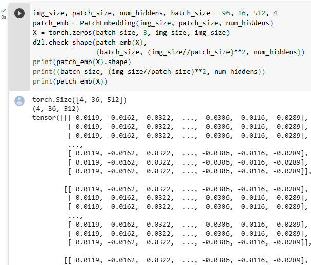
In the following example, taking images with height and width of img_size as inputs, the patch embedding outputs (img_size//patch_size)**2 patches that are linearly projected to vectors of length num_hiddens.
다음 예에서 높이와 너비가 img_size인 이미지를 입력으로 가져오면 패치 포함 출력(img_size//patch_size)**2 패치가 길이 num_hiddens의 벡터에 선형 투영됩니다.
img_size, patch_size, num_hiddens, batch_size = 96, 16, 512, 4
patch_emb = PatchEmbedding(img_size, patch_size, num_hiddens)
X = torch.zeros(batch_size, 3, img_size, img_size)
d2l.check_shape(patch_emb(X),
                (batch_size, (img_size//patch_size)**2, num_hiddens))
위 코드는 PatchEmbedding 클래스를 사용하여 이미지 데이터를 패치 임베딩으로 변환하고, 그 결과의 형태를 확인하는 과정을 나타냅니다.
- img_size, patch_size, num_hiddens, batch_size 변수들은 이미지 크기, 패치 크기, 임베딩 차원, 그리고 배치 크기를 설정합니다. 예를 들어 img_size가 96이면 이미지의 높이와 너비가 각각 96 픽셀로 가정됩니다.
- PatchEmbedding 클래스의 객체 patch_emb를 생성합니다. 생성자에는 이미지 크기, 패치 크기, 그리고 임베딩 차원이 전달됩니다.
- X는 형태가 (batch_size, 3, img_size, img_size)인 텐서로, 배치 크기만큼의 이미지 데이터를 나타냅니다. 여기서 3은 이미지의 채널 수를 나타냅니다. (예: 컬러 이미지의 경우 RGB 채널)
- patch_emb(X)는 입력 이미지 X를 PatchEmbedding 클래스로 전달하여 패치 임베딩을 계산합니다. 결과로 얻은 텐서는 (batch_size, (img_size//patch_size)^2, num_hiddens) 형태를 가지게 됩니다. 이는 배치 크기, 패치 수, 그리고 각 패치의 임베딩 차원을 나타냅니다.
- d2l.check_shape 함수는 실제로 계산된 결과와 기대하는 결과의 형태가 일치하는지 확인합니다. 기대하는 결과의 형태는 (batch_size, (img_size//patch_size)^2, num_hiddens)입니다.
11.8.3. Vision Transformer Encoder
The MLP of the vision Transformer encoder is slightly different from the position-wise FFN of the original Transformer encoder (see Section 11.7.2). First, here the activation function uses the Gaussian error linear unit (GELU), which can be considered as a smoother version of the ReLU (Hendrycks and Gimpel, 2016). Second, dropout is applied to the output of each fully connected layer in the MLP for regularization.
비전 Transformer 엔코더의 MLP는 원래 Transformer 엔코더의 position-wise FFN과 약간 다릅니다(섹션 11.7.2 참조). 먼저 여기에서 활성화 함수는 ReLU의 부드러운 버전으로 간주될 수 있는 GELU(Gaussian error linear unit)를 사용합니다(Hendrycks and Gimpel, 2016). 둘째, 정규화를 위해 MLP의 각 fully connected layer의 출력에 드롭아웃이 적용됩니다.
class ViTMLP(nn.Module):
    def __init__(self, mlp_num_hiddens, mlp_num_outputs, dropout=0.5):
        super().__init__()
        self.dense1 = nn.LazyLinear(mlp_num_hiddens)
        self.gelu = nn.GELU()
        self.dropout1 = nn.Dropout(dropout)
        self.dense2 = nn.LazyLinear(mlp_num_outputs)
        self.dropout2 = nn.Dropout(dropout)

    def forward(self, x):
        return self.dropout2(self.dense2(self.dropout1(self.gelu(
            self.dense1(x)))))
위 코드는 ViT (Vision Transformer) 모델의 MLP (Multi-Layer Perceptron) 레이어를 정의한 ViTMLP 클래스를 나타냅니다.
- mlp_num_hiddens은 MLP의 은닉 유닛 수를, mlp_num_outputs는 출력 차원 수를 의미합니다. dropout은 드롭아웃 비율을 설정하는 파라미터로 기본값은 0.5입니다.
- ViTMLP 클래스의 생성자에서는 MLP의 레이어들과 활성화 함수인 GELU(Gaussian Error Linear Unit)를 설정합니다. GELU는 비선형 활성화 함수로 사용됩니다.
- forward 메서드는 입력 데이터 x를 받아서 MLP 레이어들을 통과시켜 출력을 반환합니다.
- 실행 순서:
- self.dense1(x) : 첫 번째 fully connected 레이어를 통과한 결과
- self.gelu(...) : GELU 활성화 함수를 적용한 결과
- self.dropout1(...) : 첫 번째 드롭아웃 레이어를 통과한 결과
- self.dense2(...) : 두 번째 fully connected 레이어를 통과한 결과
- self.dropout2(...) : 두 번째 드롭아웃 레이어를 통과한 최종 출력
결과적으로, forward 메서드를 통해 입력 x가 MLP를 통과하고 드롭아웃까지 적용된 출력이 반환됩니다. 이렇게 정의된 ViTMLP 클래스는 ViT 모델 내에서 MLP 레이어로 활용될 수 있습니다.
The vision Transformer encoder block implementation just follows the pre-normalization design in Fig. 11.8.1, where normalization is applied right before multi-head attention or the MLP. In contrast to post-normalization (“add & norm” in Fig. 11.7.1), where normalization is placed right after residual connections, pre-normalization leads to more effective or efficient training for Transformers (Baevski and Auli, 2018, Wang et al., 2019, Xiong et al., 2020).
vision Transformer encoder block implementation은 그림 11.8.1의 pre-normalization 설계를 따르며 정규화가 multi-head attention 또는 MLP 직전에 적용됩니다. residual connections 바로 뒤에 정규화가 배치되는 post-normalization(그림 11.7.1의 "추가 및 규범")와 달리 pre-normalization 는 트랜스포머에 대한 보다 효과적이고 효율적인 교육으로 이어집니다(Baevski and Auli, 2018, Wang et al., 2019, Xiong et al., 2020).
class ViTBlock(nn.Module):
    def __init__(self, num_hiddens, norm_shape, mlp_num_hiddens,
                 num_heads, dropout, use_bias=False):
        super().__init__()
        self.ln1 = nn.LayerNorm(norm_shape)
        self.attention = d2l.MultiHeadAttention(num_hiddens, num_heads,
                                                dropout, use_bias)
        self.ln2 = nn.LayerNorm(norm_shape)
        self.mlp = ViTMLP(mlp_num_hiddens, num_hiddens, dropout)

    def forward(self, X, valid_lens=None):
        X = X + self.attention(*([self.ln1(X)] * 3), valid_lens)
        return X + self.mlp(self.ln2(X))
위 코드는 ViT (Vision Transformer) 모델의 블록을 정의한 ViTBlock 클래스를 나타냅니다.
- num_hiddens은 블록 내에서의 은닉 유닛 수를, norm_shape은 Layer Normalization을 위한 모양을, mlp_num_hiddens는 MLP의 은닉 유닛 수를, num_heads는 Multi-Head Attention의 헤드 개수를, dropout은 드롭아웃 비율을 나타냅니다. use_bias는 사용할 경우 편향을 사용하는지 여부를 나타내는 불리언 값입니다.
- ViTBlock 클래스의 생성자에서는 레이어 정규화(nn.LayerNorm)와 Multi-Head Attention(d2l.MultiHeadAttention) 그리고 MLP(ViTMLP)을 설정합니다.
- forward 메서드는 입력 데이터 X와 필요한 경우의 유효한 길이(valid_lens)를 받아서 블록을 통과시키고 출력을 반환합니다.
- 실행 순서:
- self.ln1(X) : 입력 데이터에 레이어 정규화를 적용한 결과
- self.attention(...): Multi-Head Attention 레이어를 통과시킨 결과
- self.ln2(X): 입력 데이터에 레이어 정규화를 다시 적용한 결과
- self.mlp(...): MLP 레이어를 통과시킨 결과
- X + ...과 X + ...: 위 두 결과를 원본 입력 데이터에 더한 최종 출력
이렇게 정의된 ViTBlock 클래스는 Vision Transformer의 핵심 구성 요소 중 하나인 블록을 나타내며, 입력 데이터를 Multi-Head Attention과 MLP 레이어를 거치면서 변환하는 역할을 합니다.
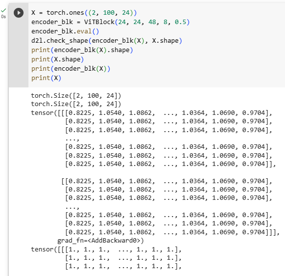
Same as in Section 11.7.4, any vision Transformer encoder block does not change its input shape.
섹션 11.7.4에서와 마찬가지로 모든 비전 Transformer 인코더 블록은 입력 모양을 변경하지 않습니다.
X = torch.ones((2, 100, 24))
encoder_blk = ViTBlock(24, 24, 48, 8, 0.5)
encoder_blk.eval()
d2l.check_shape(encoder_blk(X), X.shape)
위 코드는 ViTBlock 클래스를 활용하여 입력 데이터를 처리하는 과정을 보여주고 있습니다.
- X = torch.ones((2, 100, 24)) : 크기가 (2, 100, 24)인 입력 데이터 생성. 이는 배치 크기가 2이고, 시퀀스 길이가 100이며, 피처 차원이 24인 데이터를 의미합니다.
- encoder_blk = ViTBlock(24, 24, 48, 8, 0.5) : ViTBlock 클래스의 인스턴스를 생성합니다. 인자로는 num_hiddens, norm_shape, mlp_num_hiddens, num_heads, dropout을 제공하여 블록의 설정을 정의합니다.
- encoder_blk.eval() : 블록을 평가 모드로 설정합니다. 평가 모드에서는 드롭아웃과 같이 학습 시에만 적용되는 연산들이 비활성화됩니다.
- d2l.check_shape(encoder_blk(X), X.shape) : 생성한 encoder_blk에 입력 데이터 X를 전달하여 블록을 통과시킨 결과의 크기를 확인합니다. 이 결과가 입력 데이터의 크기와 동일해야 합니다.
즉, 위 코드는 ViTBlock 클래스로 생성한 블록에 입력 데이터를 넣고, 해당 블록을 통과시킨 결과의 크기가 입력 데이터의 크기와 일치하는지 확인하는 예시를 보여줍니다.
11.8.4. Putting It All Together
The forward pass of vision Transformers below is straightforward. First, input images are fed into an PatchEmbedding instance, whose output is concatenated with the “<cls>” token embedding. They are summed with learnable positional embeddings before dropout. Then the output is fed into the Transformer encoder that stacks num_blks instances of the ViTBlock class. Finally, the representation of the “<cls>” token is projected by the network head.
아래의 vision Transformers의 forward pass는 직관적입니다. 먼저 입력 이미지는 PatchEmbedding 인스턴스로 공급되며 출력은 "<cls>" 토큰 임베딩과 연결됩니다. 드롭아웃 전에 학습 가능한 positional embeddings으로 합산됩니다. 그런 다음 출력은 ViTBlock 클래스의 num_blks 인스턴스를 쌓는 Transformer 인코더로 공급됩니다. 마지막으로 “<cls>” 토큰의 representation 은 network head에 의해 투영됩니다.
class ViT(d2l.Classifier):
    """Vision Transformer."""
    def __init__(self, img_size, patch_size, num_hiddens, mlp_num_hiddens,
                 num_heads, num_blks, emb_dropout, blk_dropout, lr=0.1,
                 use_bias=False, num_classes=10):
        super().__init__()
        self.save_hyperparameters()
        self.patch_embedding = PatchEmbedding(
            img_size, patch_size, num_hiddens)
        self.cls_token = nn.Parameter(torch.zeros(1, 1, num_hiddens))
        num_steps = self.patch_embedding.num_patches + 1  # Add the cls token
        # Positional embeddings are learnable
        self.pos_embedding = nn.Parameter(
            torch.randn(1, num_steps, num_hiddens))
        self.dropout = nn.Dropout(emb_dropout)
        self.blks = nn.Sequential()
        for i in range(num_blks):
            self.blks.add_module(f"{i}", ViTBlock(
                num_hiddens, num_hiddens, mlp_num_hiddens,
                num_heads, blk_dropout, use_bias))
        self.head = nn.Sequential(nn.LayerNorm(num_hiddens),
                                  nn.Linear(num_hiddens, num_classes))

    def forward(self, X):
        X = self.patch_embedding(X)
        X = torch.cat((self.cls_token.expand(X.shape[0], -1, -1), X), 1)
        X = self.dropout(X + self.pos_embedding)
        for blk in self.blks:
            X = blk(X)
        return self.head(X[:, 0])
위 코드는 ViT 클래스를 정의하여 Vision Transformer 모델을 생성하는 과정을 보여주고 있습니다.
- class ViT(d2l.Classifier): : d2l.Classifier를 상속하는 ViT 클래스를 정의합니다. 이 클래스는 Vision Transformer 모델을 나타냅니다.
- def __init__(self, img_size, patch_size, num_hiddens, mlp_num_hiddens, num_heads, num_blks, emb_dropout, blk_dropout, lr=0.1, use_bias=False, num_classes=10): : 클래스 생성자입니다. 모델의 매개변수를 초기화하고 모델 구성을 설정합니다.
- self.save_hyperparameters() : 클래스 내에서 정의된 하이퍼파라미터를 저장합니다.
- self.patch_embedding = PatchEmbedding(img_size, patch_size, num_hiddens) : PatchEmbedding 클래스를 활용하여 이미지를 패치로 분할하고 임베딩하는 부분입니다.
- self.cls_token = nn.Parameter(torch.zeros(1, 1, num_hiddens)) : 클래스 토큰을 위한 파라미터로, 이미지 내에서 특별한 의미를 갖는 토큰입니다.
- self.pos_embedding = nn.Parameter(torch.randn(1, num_steps, num_hiddens)) : 위치 임베딩으로, 패치 위치에 대한 정보를 임베딩한 파라미터입니다.
- self.dropout = nn.Dropout(emb_dropout) : 입력 임베딩에 대한 드롭아웃을 정의합니다.
- self.blks = nn.Sequential() : 여러 개의 ViTBlock 레이어를 포함하는 시퀀셜 레이어를 정의합니다.
- for i in range(num_blks): : 지정한 개수만큼 ViTBlock을 생성하여 self.blks에 추가합니다.
- self.head = nn.Sequential(nn.LayerNorm(num_hiddens), nn.Linear(num_hiddens, num_classes)) : 분류를 위한 레이어를 정의합니다. 클래스 개수에 맞게 선형 레이어를 설정합니다.
- def forward(self, X): : 모델의 순전파 연산을 정의합니다.
- X = self.patch_embedding(X) : 입력 이미지를 패치 임베딩으로 변환합니다.
- X = torch.cat((self.cls_token.expand(X.shape[0], -1, -1), X), 1) : 클래스 토큰을 임베딩된 패치와 연결합니다.
- X = self.dropout(X + self.pos_embedding) : 입력 임베딩과 위치 임베딩을 더하고 드롭아웃을 적용합니다.
- for blk in self.blks: : 모델 내의 모든 ViTBlock에 대해 루프를 실행하여 순차적으로 블록을 통과시킵니다.
- return self.head(X[:, 0]) : 최종 결과를 분류 레이어에 통과시켜 예측 결과를 반환합니다.
이렇게 정의된 ViT 클래스는 입력 이미지에 대한 Vision Transformer 모델을 생성하고 해당 이미지의 클래스를 예측할 수 있는 모델을 만드는 데 사용될 수 있습니다.
11.8.5. Training
Training a vision Transformer on the Fashion-MNIST dataset is just like how CNNs were trained in Section 8.
Fashion-MNIST 데이터 세트로 비전 Transformer를 교육하는 것은 섹션 8에서 CNN을 교육한 것과 같습니다.
img_size, patch_size = 96, 16
num_hiddens, mlp_num_hiddens, num_heads, num_blks = 512, 2048, 8, 2
emb_dropout, blk_dropout, lr = 0.1, 0.1, 0.1
model = ViT(img_size, patch_size, num_hiddens, mlp_num_hiddens, num_heads,
            num_blks, emb_dropout, blk_dropout, lr)
trainer = d2l.Trainer(max_epochs=10, num_gpus=1)
data = d2l.FashionMNIST(batch_size=128, resize=(img_size, img_size))
trainer.fit(model, data)
위 코드는 Vision Transformer 모델을 생성하고 FashionMNIST 데이터셋을 사용하여 모델을 학습시키는 과정을 보여주고 있습니다.
- img_size, patch_size = 96, 16 : 이미지 크기와 패치 크기를 설정합니다.
- num_hiddens, mlp_num_hiddens, num_heads, num_blks = 512, 2048, 8, 2 : 모델의 하이퍼파라미터인 은닉 유닛 수, MLP 은닉 유닛 수, 어텐션 헤드 수, 블록 수를 설정합니다.
- emb_dropout, blk_dropout, lr = 0.1, 0.1, 0.1 : 입력 임베딩 드롭아웃 비율, 블록 드롭아웃 비율, 학습률을 설정합니다.
- model = ViT(img_size, patch_size, num_hiddens, mlp_num_hiddens, num_heads, num_blks, emb_dropout, blk_dropout, lr) : 위에서 정의한 하이퍼파라미터들을 사용하여 ViT 모델을 생성합니다.
- trainer = d2l.Trainer(max_epochs=10, num_gpus=1) : 학습을 위한 트레이너를 생성합니다. 최대 에포크 수와 GPU 개수를 설정합니다.
- data = d2l.FashionMNIST(batch_size=128, resize=(img_size, img_size)) : FashionMNIST 데이터셋을 생성합니다. 배치 크기와 이미지 리사이즈 크기를 설정합니다.
- trainer.fit(model, data) : 생성한 모델과 데이터셋을 이용하여 학습을 수행합니다. 트레이너의 fit 메서드를 사용하여 모델을 학습시킵니다.
이렇게 정의된 코드는 Vision Transformer 모델을 생성하고 FashionMNIST 데이터셋을 사용하여 모델을 학습시키는 예시를 보여줍니다.
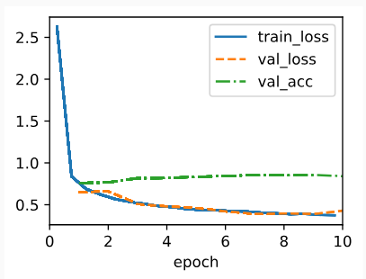
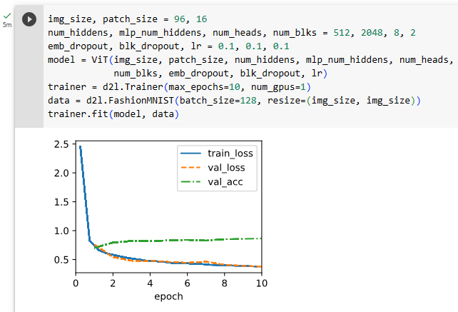
11.8.6. Summary and Discussion
You may notice that for small datasets like Fashion-MNIST, our implemented vision Transformer does not outperform the ResNet in Section 8.6. Similar observations can be made even on the ImageNet dataset (1.2 million images). This is because Transformers lack those useful principles in convolution, such as translation invariance and locality (Section 7.1). However, the picture changes when training larger models on larger datasets (e.g., 300 million images), where vision Transformers outperform ResNets by a large margin in image classification, demonstrating intrinsic superiority of Transformers in scalability (Dosovitskiy et al., 2021). The introduction of vision Transformers has changed the landscape of network design for modeling image data. They were soon shown effective on the ImageNet dataset with data-efficient training strategies of DeiT (Touvron et al., 2021). However, quadratic complexity of self-attention (Section 11.6) makes the Transformer architecture less suitable for higher-resolution images. Towards a general-purpose backbone network in computer vision, Swin Transformers addressed the quadratic computational complexity with respect to image size (Section 11.6.2) and added back convolution-like priors, extending the applicability of Transformers to a range of computer vision tasks beyond image classification with state-of-the-art results (Liu et al., 2021).
Fashion-MNIST와 같은 작은 데이터 세트의 경우 구현된 비전 Transformer가 섹션 8.6의 ResNet보다 성능이 좋지 않음을 알 수 있습니다. ImageNet 데이터 세트(120만 이미지)에서도 비슷한 관찰이 가능합니다. Transformers에는 변환 불변성 및 지역성(섹션 7.1)과 같은 컨볼루션의 유용한 원칙이 없기 때문입니다. 그러나 더 큰 데이터 세트(예: 3억 개의 이미지)에서 더 큰 모델을 교육할 때 그림이 변경됩니다. 여기서 비전 트랜스포머는 이미지 분류에서 ResNets를 훨씬 능가하여 확장성에서 트랜스포머의 본질적인 우월성을 보여줍니다(Dosovitskiy et al., 2021). 비전 트랜스포머의 도입으로 이미지 데이터 모델링을 위한 네트워크 설계의 환경이 바뀌었습니다. DeiT(Touvron et al., 2021)의 데이터 효율적인 교육 전략을 사용하여 ImageNet 데이터 세트에서 곧 효과적인 것으로 나타났습니다. 그러나 self-attention의 2차 복잡도(11.6절)는 Transformer 아키텍처를 고해상도 이미지에 적합하지 않게 만듭니다. 컴퓨터 비전의 범용 백본 네트워크를 향하기 위한 노력 중 Swin Transformers는 이미지 크기(섹션 11.6.2)와 관련하여 2차 계산 복잡성을 해결하고 convolution-like priors을 다시 추가하여 최신 결과로 이미지 분류를 넘어 다양한 컴퓨터 비전 작업으로 Transformers의 적용 가능성을 확장했습니다. (리우 외, 2021).
Swin Transformers 란?
Swin Transformer는 "Shifted Window Transformer"의 약자로, 컴퓨터 비전 분야에서 자연어 처리 모델인 Transformer 아키텍처를 적용한 최신의 딥 러닝 모델입니다. Swin Transformer는 이미지 분류, 객체 검출 및 분할과 같은 여러 컴퓨터 비전 작업에 사용되며, 특히 대규모 이미지 데이터셋에서 뛰어난 성능을 보이는 것으로 알려져 있습니다.
Swin Transformer의 주요 아이디어는 윈도우 기반의 셔틀 셋팅과 계층적 비트레이드 방법을 결합하여 높은 효율성과 확장성을 달성하는 것입니다. 이러한 방법을 사용하여 Swin Transformer는 큰 이미지를 처리하는 데도 우수한 성능을 발휘하면서도 기존의 비슷한 모델보다 더 적은 계산 비용을 필요로 합니다.
Swin Transformer의 주요 특징은 다음과 같습니다:
- Hierarchical Architecture: Swin Transformer는 여러 계층으로 구성되어 있으며, 각 계층은 점진적으로 작아지는 윈도우 크기로 이미지를 처리합니다. 이 계층 구조는 다양한 스케일의 정보를 캡처하고 전역 및 로컬 패턴을 동시에 인식할 수 있는 능력을 제공합니다.
- Shifted Windows: 기존의 이미지 분할 모델과는 달리 Swin Transformer는 이미지를 겹치는 윈도우로 나누어 처리합니다. 이것은 이미지의 모든 영역을 효율적으로 캡처하는 데 도움이 되며, 각 윈도우는 다른 윈도우의 정보를 사용하여 컨텍스트를 공유합니다.
- Tokenization and Position Embeddings: Swin Transformer는 이미지를 토큰화하고 각 토큰에 위치 정보를 포함하는 포지션 임베딩을 추가합니다. 이를 통해 이미지를 시퀀스로 처리하는 Transformer 아키텍처를 적용할 수 있습니다.
- 비트레이드 압축: Swin Transformer는 계층 간에 비트레이드 압축을 사용하여 모델의 파라미터 수를 줄이고 메모리 사용량을 최적화합니다.
Swin Transformer는 컴퓨터 비전 분야에서 주목받는 최신 모델 중 하나로, 다양한 이미지 처리 작업에 유연하게 적용할 수 있는 강력한 아키텍처입니다.
11.8.7. Exercises
- How does the value of img_size affect training time?
- Instead of projecting the “<cls>” token representation to the output, how to project the averaged patch representations? Implement this change and see how it affects the accuracy.
- Can you modify hyperparameters to improve the accuracy of the vision Transformer?
'Dive into Deep Learning > D2L Attention Mechanisms and Transformer' 카테고리의 다른 글
| D2L - 11.9. Large-Scale Pretraining with Transformers (0) | 2023.08.10 |
|---|---|
| D2L - 11.7. The Transformer Architecture (0) | 2023.08.09 |
| D2L - 11.6. Self-Attention and Positional Encoding (0) | 2023.08.09 |
| D2L - 11.5. Multi-Head Attention (0) | 2023.08.08 |
| D2L - 11.4. The Bahdanau Attention Mechanism (0) | 2023.08.08 |
| D2L - 11.3. Attention Scoring Functions (0) | 2023.08.07 |
| D2L - 11.2. Attention Pooling by Similarity (0) | 2023.08.06 |
| D2L - 11.1. Queries, Keys, and Values (0) | 2023.08.05 |
| D2L - 11. Attention Mechanisms and Transformers (0) | 2023.08.03 |