

https://d2l.ai/chapter_hyperparameter-optimization/sh-intro.html
19.4. Multi-Fidelity Hyperparameter Optimization — Dive into Deep Learning 1.0.3 documentation
d2l.ai
19.4. Multi-Fidelity Hyperparameter Optimization
Training neural networks can be expensive even on moderate size datasets. Depending on the configuration space (Section 19.1.1.2), hyperparameter optimization requires tens to hundreds of function evaluations to find a well-performing hyperparameter configuration. As we have seen in Section 19.3, we can significantly speed up the overall wall-clock time of HPO by exploiting parallel resources, but this does not reduce the total amount of compute required.
적당한 크기의 데이터 세트에서도 신경망을 훈련하는 데 비용이 많이 들 수 있습니다. 구성 공간(19.1.1.2절)에 따라 하이퍼파라미터 최적화에는 성능이 좋은 하이퍼파라미터 구성을 찾기 위해 수십에서 수백 번의 함수 평가가 필요합니다. 섹션 19.3에서 살펴본 것처럼 병렬 리소스를 활용하여 HPO의 전체 벽시계 시간을 크게 단축할 수 있지만 이것이 필요한 총 컴퓨팅 양을 줄이지는 않습니다.
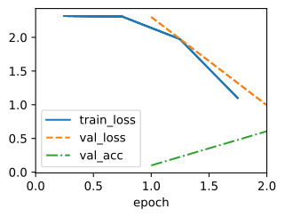
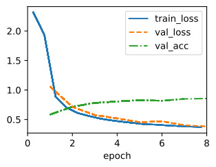
In this section, we will show how the evaluation of hyperparameter configurations can be sped up. Methods such as random search allocate the same amount of resources (e.g., number of epochs, training data points) to each hyperparameter evaluation. Fig. 19.4.1 depicts learning curves of a set of neural networks trained with different hyperparameter configurations. After a few epochs we are already able to visually distinguish between well-performing and suboptimal configurations. However, the learning curves are noisy, and we might still require the full amount of 100 epochs to identify the best performing one.
이 섹션에서는 하이퍼파라미터 구성의 평가 속도를 높이는 방법을 보여줍니다. 무작위 검색과 같은 방법은 각 하이퍼파라미터 평가에 동일한 양의 리소스(예: 시대 수, 교육 데이터 포인트)를 할당합니다. 그림 19.4.1은 다양한 하이퍼파라미터 구성으로 훈련된 신경망 세트의 학습 곡선을 보여줍니다. 몇 번의 시대가 지나면 이미 성능이 좋은 구성과 최적이 아닌 구성을 시각적으로 구분할 수 있습니다. 그러나 학습 곡선에는 잡음이 많으므로 최고의 성과를 내는 것을 식별하려면 여전히 100개의 에포크가 필요할 수 있습니다.

Multi-fidelity hyperparameter optimization allocates more resources to promising configurations and stop evaluations of poorly performing ones early. This speeds up the optimization process, since we can try a larger number of configurations for the same total amount of resources.
다중 충실도 하이퍼파라미터 최적화는 유망한 구성에 더 많은 리소스를 할당하고 성능이 낮은 구성에 대한 평가를 조기에 중지합니다. 동일한 총 리소스 양에 대해 더 많은 수의 구성을 시도할 수 있으므로 최적화 프로세스 속도가 빨라집니다.
More formally, we expand our definition in Section 19.1.1, such that our objective function f(x,r) gets an additional input r∈[r min,r max], specifying the amount of resources that we are willing to spend for the evaluation of configuration x. We assume that the error f(x,r) decreases with r, whereas the computational cost c(x,r) increases. Typically, r represents the number of epochs for training the neural network, but it could also be the training subset size or the number of cross-validation folds.
보다 공식적으로, 목적 함수 f(x,r)가 추가 입력 r∈[r min,r max]를 얻도록 섹션 19.1.1의 정의를 확장하여 지출하려는 자원의 양을 지정합니다. 구성 x의 평가. 오류 f(x,r)는 r에 따라 감소하는 반면 계산 비용 c(x,r)은 증가한다고 가정합니다. 일반적으로 r은 신경망 훈련을 위한 에포크 수를 나타내지만 훈련 하위 집합 크기 또는 교차 검증 접기 수일 수도 있습니다.
from collections import defaultdict
import numpy as np
from scipy import stats
from d2l import torch as d2l

d2l.set_figsize()
위의 코드는 Python 라이브러리와 도구를 가져오고, 그림의 크기를 설정하는 부분입니다.
- from collections import defaultdict: Python의 내장 모듈인 collections에서 defaultdict 클래스를 가져옵니다. defaultdict는 기본값(default)을 가진 딕셔너리(dictionary)를 생성하는데 사용됩니다.
- import numpy as np: NumPy 라이브러리를 가져옵니다. NumPy는 과학적 계산을 위한 파이썬 라이브러리로 배열(array)과 행렬(matrix) 연산을 지원합니다. np는 NumPy를 짧게 참조하기 위한 별칭(alias)입니다.
- from scipy import stats: SciPy 라이브러리에서 stats 모듈을 가져옵니다. SciPy는 과학적 계산을 위한 다양한 기능을 제공하는 라이브러리로, 통계 분석과 관련된 함수와 도구를 포함하고 있습니다.
- from d2l import torch as d2l: "d2l" 라이브러리에서 "torch" 모듈을 가져오고, "d2l"을 짧게 참조하기 위한 별칭으로 사용합니다.
- d2l.set_figsize(): "d2l" 라이브러리에서 제공하는 함수인 set_figsize()를 호출하여 그림(플롯)의 크기를 설정합니다. 이 함수는 시각화에서 그림의 크기를 조정하는 데 사용됩니다. 크기를 따로 지정하지 않으면 기본 크기로 설정됩니다.
이 코드는 라이브러리를 가져와 사용할 수 있도록 하고, 그림의 크기를 설정하여 나중에 생성할 그래프나 플롯의 크기를 지정합니다.
Multi-Fidelity Hyperparameter Optimization이란? (GPT 3.5 답변)
**다중 신뢰도 하이퍼파라미터 최적화(Multi-Fidelity Hyperparameter Optimization)**는 하이퍼파라미터 최적화를 위한 고급 기술 중 하나로, 기계 학습 모델을 효율적으로 튜닝하기 위해 여러 가지 신뢰도 또는 리소스 수준에서 모델을 평가하는 방법입니다. 일반적으로 이러한 접근 방식은 계산 비용이 높은 고신뢰도(또는 고 리소스) 평가와 계산 비용이 낮은 저신뢰도(또는 저 리소스) 평가를 혼합하여 사용합니다.
다중 신뢰도 하이퍼파라미터 최적화의 핵심 아이디어는 다음과 같습니다.
- 고신뢰도 평가 (High-Fidelity Evaluation): 높은 신뢰도를 가진 평가는 모델의 성능을 정확하게 측정합니다. 이것은 많은 계산 리소스와 시간을 필요로 합니다. 예를 들어, 모든 훈련 데이터와 에포크 수를 늘리는 것과 같이 모델을 더 오랫동안 훈련하는 것이 포함될 수 있습니다.
- 저신뢰도 평가 (Low-Fidelity Evaluation): 저신뢰도 평가는 고신뢰도 평가보다 빠르게 수행됩니다. 예를 들어, 더 적은 훈련 데이터를 사용하거나 적은 에포크로 모델을 훈련하는 것이 이에 해당합니다.
- 리소스 관리: 다중 신뢰도 하이퍼파라미터 최적화는 제한된 계산 리소스 또는 시간 내에서 가장 효율적으로 최적화를 수행하려는 목표를 가지고 있습니다. 이를 위해 리소스를 고정된 신뢰도 평가와 저신뢰도 평가 사이에서 분배합니다.
- 바람직한 트레이드오프 탐색: 목표는 최적의 하이퍼파라미터 설정을 찾는 것이지만, 모든 경우에 고신뢰도 평가를 수행하는 것은 현실적이지 않을 수 있습니다. 따라서 가용한 리소스 내에서 가능한 한 많은 하이퍼파라미터 설정을 평가하여 최상의 트레이드오프를 찾습니다.
- 자동화된 하이퍼파라미터 선택: 다중 신뢰도 하이퍼파라미터 최적화는 주어진 리소스 내에서 자동으로 하이퍼파라미터를 선택하고 평가합니다. 이것은 기계 학습 엔지니어 또는 데이터 과학자에게 매우 유용합니다.
다중 신뢰도 하이퍼파라미터 최적화는 하이퍼파라미터 튜닝 과정을 가속화하고 계산 리소스를 효율적으로 활용하면서 최상의 하이퍼파라미터 설정을 찾는 데 도움을 줍니다. 이 방법은 기계 학습 모델의 성능을 최대화하는 데 중요합니다.
19.4.1. Successive Halving
One of the simplest ways to adapt random search to the multi-fidelity setting is successive halving (Jamieson and Talwalkar, 2016, Karnin et al., 2013). The basic idea is to start with N configurations, for example randomly sampled from the configuration space, and to train each of them for r min epochs only. We then discard a fraction of the worst performing trials and train the remaining ones for longer. Iterating this process, fewer trials run for longer, until at least one trial reaches r max epochs.
다중 충실도 설정에 무작위 검색을 적용하는 가장 간단한 방법 중 하나는 연속적인 반감기입니다(Jamieson and Talwalkar, 2016, Karnin et al., 2013). 기본 아이디어는 예를 들어 구성 공간에서 무작위로 샘플링된 N 구성으로 시작하고 각 구성을 r min epoch 동안만 훈련하는 것입니다. 그런 다음 성능이 가장 낮은 시험 중 일부를 버리고 나머지 시험을 더 오랫동안 훈련합니다. 이 프로세스를 반복하면 적어도 하나의 시도가 r 최대 에포크에 도달할 때까지 더 적은 수의 시도가 더 오랫동안 실행됩니다.
More formally, consider a minimum budget r min (for example 1 epoch), a maximum budget r max, for example max_epochs in our previous example, and a halving constant η∈{2,3,…}. For simplicity, assume that r max = r min η**k, with K∈‖ . The number of initial configurations is then N=η**k. Let us define the set of rungs R = {r min, r min η, r min η**2,…,r max}.
보다 공식적으로는 최소 예산 r min(예: 1 epoch), 최대 예산 r max(예: 이전 예의 max_epochs) 및 반감 상수 eta∈{2,3,…}를 고려합니다. 단순화를 위해 r max = r min θ**k, K∈ʼ 라고 가정합니다. 그러면 초기 구성 수는 N=θ**k입니다. 단계 세트 R = {r min, r min eta, r min eta**2,…,r max}를 정의해 보겠습니다.
One round of successive halving proceeds as follows. We start with running N trials until the first rung r min. Sorting the validation errors, we keep the top 1/η fraction (which amounts to η**k−1 configurations) and discard all the rest. The surviving trials are trained for the next rung (r min η epochs), and the process is repeated. At each rung, a 1/η fraction of trials survives and their training continues with a η times larger budget. With this particular choice of N, only a single trial will be trained to the full budget r max. Once such a round of successive halving is done, we start the next one with a new set of initial configurations, iterating until the total budget is spent.
한 라운드의 연속적인 반감기는 다음과 같이 진행됩니다. 첫 번째 rung r min까지 N번 시도를 실행하는 것으로 시작합니다. 검증 오류를 정렬하면서 상위 1/eta 부분(eta**k−1 구성에 해당)을 유지하고 나머지는 모두 삭제합니다. 살아남은 시도는 다음 단계(r min θ epochs)에 대해 훈련되고 프로세스가 반복됩니다. 각 단계에서 시행의 1/θ 비율이 살아남고 해당 훈련은 θ배 더 큰 예산으로 계속됩니다. 이 특정 N 선택을 사용하면 단일 시도만 전체 예산 r max로 학습됩니다. 이러한 연속적인 반감기가 완료되면 새로운 초기 구성 세트로 다음 단계를 시작하여 총 예산이 소비될 때까지 반복합니다.

Successive Halving 이란? (GPT 3.5 답변)
Successive Halving은 하이퍼파라미터 최적화에서 사용되는 고급 기술 중 하나입니다. 이 방법은 많은 하이퍼파라미터 구성을 효율적으로 평가하고 가장 우수한 하이퍼파라미터 구성을 찾는 데 도움을 줍니다.
Successive Halving은 다음 단계로 구성됩니다:
- 초기 라운드 (Initial Round): 먼저 모든 하이퍼파라미터 구성을 동일한 리소스 또는 시간 내에서 평가합니다. 이 단계에서는 많은 하이퍼파라미터 구성을 아직 유망한지 판단하지 않고 각각을 동등하게 다룹니다.
- 선택 (Selection): 초기 라운드에서 우수한 일부 하이퍼파라미터 구성만 선택합니다. 일반적으로 이것은 상위 N개 구성을 선택하는 것으로 시작합니다. 이 선택 기준은 주로 목표 지표 (예: 정확도 또는 손실)을 기반으로 합니다.
- 제거 (Elimination): 선택된 하이퍼파라미터 구성 중 일부를 제거합니다. 제거 기준은 각 구성의 상대적 효용성을 평가하는 데 사용됩니다. 이것은 효율성을 높이기 위한 주요 단계로, 낮은 성능을 보이는 하이퍼파라미터 구성을 제거하고 리소스를 더 높은 효과적인 평가로 할당하는 데 도움을 줍니다.
- 라운드 반복 (Iteration): 선정된 하이퍼파라미터 구성들을 다음 라운드로 이동시킵니다. 이제 리소스 또는 시간을 더욱 증가시켜 더 정확한 평가를 수행합니다. 이 프로세스는 몇 라운드에 걸쳐 반복됩니다.
Successive Halving은 초기에 무작위로 선택된 하이퍼파라미터 구성들을 점진적으로 걸러내고 가장 우수한 구성을 찾기 위해 리소스를 최적으로 활용하는 방법 중 하나입니다. 이 방법은 계산 리소스를 효율적으로 활용하면서도 최상의 하이퍼파라미터 설정을 찾는 데 도움을 줍니다.
We subclass the HPOScheduler base class from Section 19.2 in order to implement successive halving, allowing for a generic HPOSearcher object to sample configurations (which, in our example below, will be a RandomSearcher). Additionally, the user has to pass the minimum resource r min, the maximum resource r max and η as input. Inside our scheduler, we maintain a queue of configurations that still need to be evaluated for the current rung ri. We update the queue every time we jump to the next rung.
연속적인 절반 분할을 구현하기 위해 섹션 19.2에서 HPOScheduler 기본 클래스를 서브클래싱하여 일반 HPOSearcher 객체가 샘플 구성(아래 예에서는 RandomSearcher가 됨)을 허용합니다. 또한 사용자는 최소 리소스 r min, 최대 리소스 r max 및 eta를 입력으로 전달해야 합니다. 스케줄러 내에서는 현재 단계에 대해 여전히 평가해야 하는 구성 대기열을 유지 관리합니다. 다음 단계로 이동할 때마다 대기열을 업데이트합니다.
class SuccessiveHalvingScheduler(d2l.HPOScheduler):  #@save
    def __init__(self, searcher, eta, r_min, r_max, prefact=1):
        self.save_hyperparameters()
        # Compute K, which is later used to determine the number of configurations
        self.K = int(np.log(r_max / r_min) / np.log(eta))
        # Define the rungs
        self.rung_levels = [r_min * eta ** k for k in range(self.K + 1)]
        if r_max not in self.rung_levels:
            # The final rung should be r_max
            self.rung_levels.append(r_max)
            self.K += 1
        # Bookkeeping
        self.observed_error_at_rungs = defaultdict(list)
        self.all_observed_error_at_rungs = defaultdict(list)
        # Our processing queue
        self.queue = []
위의 코드는 SuccessiveHalvingScheduler라는 클래스를 정의하는 부분입니다. 이 클래스는 하이퍼파라미터 최적화 실험을 위한 스케줄러로 사용됩니다.
- def __init__(self, searcher, eta, r_min, r_max, prefact=1):: SuccessiveHalvingScheduler 클래스의 초기화 메서드입니다. 이 클래스는 여러 하이퍼파라미터를 받아 초기화됩니다.
- searcher: 하이퍼파라미터 탐색기(searcher) 객체입니다.
- eta: 탐색 단계 간의 이동 비율입니다.
- r_min: 최소 리소스(예: 시간, 계산 능력)입니다.
- r_max: 최대 리소스(예: 시간, 계산 능력)입니다.
- prefact: 사전 요소(pre-factored)입니다.
- self.K = int(np.log(r_max / r_min) / np.log(eta)): K는 하이퍼파라미터 조합을 조사할 최대 횟수를 나타내는 변수입니다. eta와 리소스 범위에 따라 계산됩니다.
- self.rung_levels = [r_min * eta ** k for k in range(self.K + 1)]: rung_levels는 각 단계의 리소스 레벨을 저장하는 리스트입니다. r_min에서 시작하여 eta의 거듭제곱을 계산하여 각 단계의 리소스 레벨을 결정합니다.
- if r_max not in self.rung_levels:: r_max가 rung_levels에 포함되지 않으면, r_max를 추가합니다. 이렇게 하여 최종 단계에서도 r_max 리소스를 사용할 수 있도록 합니다.
- self.observed_error_at_rungs = defaultdict(list): observed_error_at_rungs는 각 단계에서 관찰된 에러를 저장하기 위한 딕셔너리입니다. 에러는 각 단계에서 계산되고 저장됩니다.
- self.all_observed_error_at_rungs = defaultdict(list): all_observed_error_at_rungs는 모든 실험에서 관찰된 에러를 저장하기 위한 딕셔너리입니다. 모든 실험에서 관찰된 에러를 추적합니다.
- self.queue = []: 실험을 수행하기 위한 큐(queue)를 초기화합니다. 실험 조합은 이 큐에 추가되어 순차적으로 실행됩니다.
이 클래스는 Successive Halving 알고리즘에 기반하여 하이퍼파라미터 탐색을 수행합니다. 각 단계에서 최적의 하이퍼파라미터 조합을 선택하고, 이를 기반으로 다음 단계의 실험을 수행합니다.
In the beginning our queue is empty, and we fill it with n=prefact⋅η**k configurations, which are first evaluated on the smallest rung r min. Here, prefact allows us to reuse our code in a different context. For the purpose of this section, we fix prefact=1. Every time resources become available and the HPOTuner object queries the suggest function, we return an element from the queue. Once we finish one round of successive halving, which means that we evaluated all surviving configurations on the highest resource level r max and our queue is empty, we start the entire process again with a new, randomly sampled set of configurations.
처음에는 대기열이 비어 있으며 n=prefact⋅eta**k 구성으로 채워져 가장 작은 단계 r min에서 먼저 평가됩니다. 여기서 prefact를 사용하면 다른 컨텍스트에서 코드를 재사용할 수 있습니다. 이 섹션의 목적을 위해 prefact=1을 수정합니다. 리소스를 사용할 수 있게 되고 HPOTuner 개체가 제안 기능을 쿼리할 때마다 대기열에서 요소를 반환합니다. 한 라운드의 연속적인 반감기를 마치면, 즉 가장 높은 리소스 수준 r max에서 살아남은 모든 구성을 평가하고 대기열이 비어 있으면 무작위로 샘플링된 새로운 구성 세트로 전체 프로세스를 다시 시작합니다.
@d2l.add_to_class(SuccessiveHalvingScheduler)  #@save
def suggest(self):
    if len(self.queue) == 0:
        # Start a new round of successive halving
        # Number of configurations for the first rung:
        n0 = int(self.prefact * self.eta ** self.K)
        for _ in range(n0):
            config = self.searcher.sample_configuration()
            config["max_epochs"] = self.r_min  # Set r = r_min
            self.queue.append(config)
    # Return an element from the queue
    return self.queue.pop()
위의 코드는 SuccessiveHalvingScheduler 클래스에 suggest 메서드를 추가하는 부분입니다. 이 메서드는 다음 실험에 사용할 하이퍼파라미터 조합을 제안하는 역할을 합니다.
- if len(self.queue) == 0:: 큐(queue)가 비어있는 경우, 새로운 Successive Halving 라운드를 시작합니다. 이는 다음 단계에서 실험할 하이퍼파라미터 조합을 선택하는 단계입니다.
- n0 = int(self.prefact * self.eta ** self.K): 첫 번째 단계의 실험 횟수(n0)를 계산합니다. prefact와 eta를 사용하여 최초 단계에서 실험할 하이퍼파라미터 조합의 수를 결정합니다.
- for _ in range(n0):: 계산된 실험 횟수만큼 반복하여 하이퍼파라미터 조합을 선택하고 큐에 추가합니다.
- config["max_epochs"] = self.r_min: 선택한 하이퍼파라미터 조합의 max_epochs 값을 r_min으로 설정합니다. 이렇게 하여 해당 단계에서의 최소 리소스를 사용하게 됩니다.
- self.queue.pop(): 큐에서 하이퍼파라미터 조합을 하나씩 꺼내서 반환합니다. 이 조합은 다음 실험에 사용됩니다.
이 메서드는 Successive Halving 알고리즘에 따라 다음 실험에 사용할 하이퍼파라미터 조합을 선택하고, 큐에서 해당 조합을 제거하는 역할을 합니다.
When we collected a new data point, we first update the searcher module. Afterwards we check if we already collect all data points on the current rung. If so, we sort all configurations and push the top 1/η configurations into the queue.
새로운 데이터 포인트를 수집하면 먼저 검색 모듈을 업데이트합니다. 그런 다음 현재 단계에서 모든 데이터 포인트를 이미 수집했는지 확인합니다. 그렇다면 모든 구성을 정렬하고 상위 1/eta 구성을 대기열에 푸시합니다.
@d2l.add_to_class(SuccessiveHalvingScheduler)  #@save
def update(self, config: dict, error: float, info=None):
    ri = int(config["max_epochs"])  # Rung r_i
    # Update our searcher, e.g if we use Bayesian optimization later
    self.searcher.update(config, error, additional_info=info)
    self.all_observed_error_at_rungs[ri].append((config, error))
    if ri < self.r_max:
        # Bookkeeping
        self.observed_error_at_rungs[ri].append((config, error))
        # Determine how many configurations should be evaluated on this rung
        ki = self.K - self.rung_levels.index(ri)
        ni = int(self.prefact * self.eta ** ki)
        # If we observed all configuration on this rung r_i, we estimate the
        # top 1 / eta configuration, add them to queue and promote them for
        # the next rung r_{i+1}
        if len(self.observed_error_at_rungs[ri]) >= ni:
            kiplus1 = ki - 1
            niplus1 = int(self.prefact * self.eta ** kiplus1)
            best_performing_configurations = self.get_top_n_configurations(
                rung_level=ri, n=niplus1
            )
            riplus1 = self.rung_levels[self.K - kiplus1]  # r_{i+1}
            # Queue may not be empty: insert new entries at the beginning
            self.queue = [
                dict(config, max_epochs=riplus1)
                for config in best_performing_configurations
            ] + self.queue
            self.observed_error_at_rungs[ri] = []  # Reset
위의 코드는 SuccessiveHalvingScheduler 클래스에 update 메서드를 추가하는 부분입니다. 이 메서드는 각 실험의 결과를 기반으로 다음 단계의 실험을 업데이트하고 관리합니다.
- ri = int(config["max_epochs"]): 현재 실험에서 사용한 max_epochs 값을 가져와 ri 변수에 저장합니다. 이 값은 현재 실험의 리소스 레벨을 나타냅니다.
- self.searcher.update(config, error, additional_info=info): searcher 객체를 업데이트합니다. 이는 나중에 베이지안 최적화와 같은 다른 탐색 알고리즘을 사용할 때 유용합니다.
- self.all_observed_error_at_rungs[ri].append((config, error)): 모든 실험에서 현재 리소스 레벨 ri에서 관찰된 에러를 저장합니다.
- if ri < self.r_max:: 현재 리소스 레벨이 최대 리소스 레벨 r_max보다 작은 경우에만 다음 단계의 처리를 진행합니다.
- ki = self.K - self.rung_levels.index(ri): 현재 리소스 레벨에 해당하는 단계 ki를 계산합니다.
- ni = int(self.prefact * self.eta ** ki): 현재 단계에서 평가할 실험의 수를 계산합니다.
- if len(self.observed_error_at_rungs[ri]) >= ni:: 현재 리소스 레벨에서 이미 모든 실험을 수행한 경우에는 다음 단계로 넘어갑니다.
- kiplus1 = ki - 1과 niplus1 = int(self.prefact * self.eta ** kiplus1)을 계산하여 다음 단계에서 평가할 실험의 수와 단계를 결정합니다.
- best_performing_configurations = self.get_top_n_configurations(rung_level=ri, n=niplus1): 현재 단계에서 성능이 가장 좋은 상위 niplus1개의 하이퍼파라미터 조합을 가져옵니다.
- riplus1 = self.rung_levels[self.K - kiplus1]: 다음 단계의 리소스 레벨 riplus1을 결정합니다.
- self.queue = [...] + self.queue: 다음 단계의 실험을 큐에 추가합니다. 이때, 현재 큐에 있는 실험들은 다음 단계의 리소스 레벨로 업데이트되고, 상위 성능 조합들이 추가됩니다.
- self.observed_error_at_rungs[ri] = []: 현재 단계에서 관찰된 에러를 리셋하여 다음 단계를 위한 준비를 합니다.
이 메서드는 Successive Halving 알고리즘의 핵심 로직을 구현하며, 각 실험의 결과를 바탕으로 다음 실험의 하이퍼파라미터 조합을 선택하고 큐를 관리합니다.
Configurations are sorted based on their observed performance on the current rung.
구성은 현재 단계에서 관찰된 성능을 기준으로 정렬됩니다.
@d2l.add_to_class(SuccessiveHalvingScheduler)  #@save
def get_top_n_configurations(self, rung_level, n):
    rung = self.observed_error_at_rungs[rung_level]
    if not rung:
        return []
    sorted_rung = sorted(rung, key=lambda x: x[1])
    return [x[0] for x in sorted_rung[:n]]
위의 코드는 SuccessiveHalvingScheduler 클래스에 get_top_n_configurations 메서드를 추가하는 부분입니다. 이 메서드는 주어진 리소스 레벨에서 성능이 가장 좋은 상위 n개 하이퍼파라미터 조합을 반환합니다.
- rung = self.observed_error_at_rungs[rung_level]: 주어진 리소스 레벨 rung_level에서 관찰된 모든 실험 결과를 가져옵니다.
- if not rung:: 만약 해당 리소스 레벨에서 아직 어떤 실험이 수행되지 않았다면 빈 리스트를 반환합니다.
- sorted_rung = sorted(rung, key=lambda x: x[1]): 실험 결과를 성능(에러 값)에 따라 정렬합니다.
- return [x[0] for x in sorted_rung[:n]]: 상위 n개의 실험 중 하이퍼파라미터 조합만을 반환합니다. 이는 다음 단계의 실험에 사용됩니다.
즉, get_top_n_configurations 메서드는 주어진 리소스 레벨에서 성능이 가장 좋은 하이퍼파라미터 조합을 선택하는데 사용되며, Successive Halving 알고리즘의 핵심 부분 중 하나입니다.
Let us see how successive halving is doing on our neural network example. We will use r min=2, η=2, r max=10, so that rung levels are 2,4,8,10.
신경망 예제에서 연속적인 반감기가 어떻게 수행되는지 살펴보겠습니다. r min=2, eta=2, r max=10을 사용하므로 단계 수준은 2,4,8,10이 됩니다.
min_number_of_epochs = 2
max_number_of_epochs = 10
eta = 2
num_gpus=1

config_space = {
    "learning_rate": stats.loguniform(1e-2, 1),
    "batch_size": stats.randint(32, 256),
}
initial_config = {
    "learning_rate": 0.1,
    "batch_size": 128,
}
위의 코드는 Successive Halving HPO (Hyperparameter Optimization) 알고리즘을 설정하는 부분입니다. 이 알고리즘은 하이퍼파라미터 최적화를 위해 사용되며, 주어진 리소스로 가장 좋은 하이퍼파라미터 설정을 찾는 데 도움이 됩니다. 아래는 각 설정과 변수에 대한 설명입니다.
- min_number_of_epochs (최소 에포크 수): 각 실험에서 최소 몇 번의 에포크를 실행할지를 나타냅니다. 이 값은 2로 설정되어 있습니다.
- max_number_of_epochs (최대 에포크 수): 각 실험에서 최대 몇 번의 에포크까지 실행할지를 나타냅니다. 이 값은 10으로 설정되어 있습니다.
- eta (탐색 요인): Successive Halving 알고리즘에서 리소스를 나누는 데 사용되는 요인을 나타냅니다. 이 값은 2로 설정되어 있으며, 리소스가 반으로 줄어들 때마다 실행되는 실험 수가 2배로 증가합니다.
- num_gpus (GPU 수): 사용 가능한 GPU 수를 나타냅니다. 이 예제에서는 1로 설정되어 있습니다.
- config_space (하이퍼파라미터 공간): 하이퍼파라미터 최적화를 위해 탐색할 하이퍼파라미터 공간을 정의합니다. 여기에서는 학습률(learning_rate)과 배치 크기(batch_size)를 설정하고, 각각 loguniform 및 randint 확률 분포를 사용하여 하이퍼파라미터를 탐색할 범위를 지정합니다.
- initial_config (초기 하이퍼파라미터 설정): 최초의 실험을 위해 사용되는 초기 하이퍼파라미터 설정을 나타냅니다. 이 예제에서는 학습률을 0.1로, 배치 크기를 128로 설정합니다.
이러한 설정과 변수들은 Successive Halving HPO 알고리즘을 실행하고 하이퍼파라미터 최적화를 수행하는 데 필요한 매개변수와 공간을 정의합니다.
We just replace the scheduler with our new SuccessiveHalvingScheduler.
스케줄러를 새로운 SuccessiveHalvingScheduler로 교체합니다.
searcher = d2l.RandomSearcher(config_space, initial_config=initial_config)
scheduler = SuccessiveHalvingScheduler(
    searcher=searcher,
    eta=eta,
    r_min=min_number_of_epochs,
    r_max=max_number_of_epochs,
)
tuner = d2l.HPOTuner(
    scheduler=scheduler,
    objective=d2l.hpo_objective_lenet,
)
tuner.run(number_of_trials=30)
위의 코드는 Successive Halving HPO 알고리즘을 구현하고 실행하는 부분입니다. 아래는 코드의 주요 내용에 대한 설명입니다.
- searcher: RandomSearcher는 하이퍼파라미터 탐색을 수행하는 데 사용되는 탐색자(searcher)입니다. config_space에서 정의한 하이퍼파라미터 공간을 기반으로 하이퍼파라미터 설정을 무작위로 추출하며, 초기 설정은 initial_config로 설정됩니다.
- scheduler: SuccessiveHalvingScheduler는 Successive Halving 알고리즘의 스케줄러입니다. 이 스케줄러는 searcher로부터 샘플된 하이퍼파라미터 설정을 기반으로 실험을 관리하고, eta, r_min, r_max 등을 사용하여 실험을 반복하고 스케줄링합니다.
- tuner: HPOTuner는 하이퍼파라미터 최적화를 수행하는 클래스입니다. scheduler를 통해 실험을 관리하고, objective 함수를 사용하여 각 실험의 성능을 평가하며, number_of_trials 매개변수에 지정된 횟수만큼 실험을 실행합니다.
이렇게 구성된 코드는 Successive Halving 알고리즘을 사용하여 하이퍼파라미터 최적화를 수행하며, 30회의 실험을 실행하여 최적의 하이퍼파라미터 설정을 찾습니다.
error = 0.17762434482574463, runtime = 53.576584339141846


We can visualize the learning curves of all configurations that we evaluated. Most of the configurations are stopped early and only the better performing configurations survive until r max. Compare this to vanilla random search, which would allocate r max to every configuration.
평가한 모든 구성의 학습 곡선을 시각화할 수 있습니다. 대부분의 구성은 조기에 중지되며 더 나은 성능의 구성만 r max까지 유지됩니다. 이것을 모든 구성에 r max를 할당하는 바닐라 무작위 검색과 비교해 보세요.
for rung_index, rung in scheduler.all_observed_error_at_rungs.items():
    errors = [xi[1] for xi in rung]
    d2l.plt.scatter([rung_index] * len(errors), errors)
d2l.plt.xlim(min_number_of_epochs - 0.5, max_number_of_epochs + 0.5)
d2l.plt.xticks(
    np.arange(min_number_of_epochs, max_number_of_epochs + 1),
    np.arange(min_number_of_epochs, max_number_of_epochs + 1)
)
d2l.plt.ylabel("validation error")
d2l.plt.xlabel("epochs")
위의 코드는 Successive Halving HPO 알고리즘을 통해 각 rung(레벨)에서 관찰된 검증 오차(validation error)를 시각화하는 부분입니다. 아래는 코드의 주요 내용에 대한 설명입니다.
- for rung_index, rung in scheduler.all_observed_error_at_rungs.items():: all_observed_error_at_rungs에는 각 rung 레벨에서 관찰된 검증 오차의 정보가 저장되어 있습니다. 이 코드는 각 rung에 대한 정보를 반복하며 그래프를 그립니다.
- errors = [xi[1] for xi in rung]: 각 rung에서 관찰된 검증 오차를 추출하여 errors 리스트에 저장합니다.
- d2l.plt.scatter([rung_index] * len(errors), errors): rung 레벨에 해당하는 x 좌표에 해당 오차 값을 점으로 표시하여 그래프에 추가합니다.
- d2l.plt.xlim(min_number_of_epochs - 0.5, max_number_of_epochs + 0.5): x 축의 범위를 설정합니다.
- d2l.plt.xticks(np.arange(min_number_of_epochs, max_number_of_epochs + 1), np.arange(min_number_of_epochs, max_number_of_epochs + 1)): x 축의 눈금을 설정합니다. rung 레벨에 해당하는 값들이 표시됩니다.
- d2l.plt.ylabel("validation error")와 d2l.plt.xlabel("epochs"): y 축과 x 축에 라벨을 추가합니다.
이 코드를 통해 각 rung 레벨에서 관찰된 검증 오차를 epochs(에폭)별로 시각적으로 확인할 수 있습니다.
Text(0.5, 0, 'epochs')
Finally, note some slight complexity in our implementation of SuccessiveHalvingScheduler. Say that a worker is free to run a job, and suggest is called when the current rung has almost been completely filled, but another worker is still busy with an evaluation. Since we lack the metric value from this worker, we cannot determine the top 1/η fraction to open up the next rung. On the other hand, we want to assign a job to our free worker, so it does not remain idle. Our solution is to start a new round of successive halving and assign our worker to the first trial there. However, once a rung is completed in update, we make sure to insert new configurations at the beginning of the queue, so they take precedence over configurations from the next round.
마지막으로 SuccessiveHalvingScheduler 구현이 약간 복잡하다는 점에 유의하세요. 작업자가 작업을 자유롭게 실행할 수 있고 현재 단계가 거의 완전히 채워졌을 때 제안이 호출되지만 다른 작업자는 여전히 평가로 바쁘다고 가정해 보겠습니다. 이 작업자의 메트릭 값이 부족하기 때문에 다음 단계를 열기 위한 상위 1/θ 비율을 결정할 수 없습니다. 반면에 우리는 무료 작업자에게 작업을 할당하여 유휴 상태로 남아 있지 않도록 하려고 합니다. 우리의 해결책은 새로운 연속 반감기 라운드를 시작하고 그곳에서 첫 번째 시도에 작업자를 할당하는 것입니다. 그러나 업데이트에서 단계가 완료되면 대기열 시작 부분에 새 구성을 삽입하여 다음 라운드의 구성보다 우선하도록 합니다.
19.4.2. Summary
In this section, we introduced the concept of multi-fidelity hyperparameter optimization, where we assume to have access to cheap-to-evaluate approximations of the objective function, such as validation error after a certain number of epochs of training as proxy to validation error after the full number of epochs. Multi-fidelity hyperparameter optimization allows to reduce the overall computation of the HPO instead of just reducing the wall-clock time.
이 섹션에서는 다중 충실도 하이퍼파라미터 최적화의 개념을 소개했습니다. 여기서 우리는 검증 오류에 대한 프록시로서 특정 횟수의 훈련 후 검증 오류와 같이 목적 함수의 평가하기 쉬운 근사값에 액세스할 수 있다고 가정합니다. 전체 에포크 수 이후. 다중 충실도 하이퍼파라미터 최적화를 사용하면 벽시계 시간을 줄이는 대신 HPO의 전체 계산을 줄일 수 있습니다.
We implemented and evaluated successive halving, a simple yet efficient multi-fidelity HPO algorithm.
우리는 간단하면서도 효율적인 다중 충실도 HPO 알고리즘인 연속 반감기를 구현하고 평가했습니다.
'Dive into Deep Learning > D2L Hyperparameter Optimization' 카테고리의 다른 글
| D2L - 19.5. Asynchronous Successive Halving (0) | 2023.09.10 |
|---|---|
| D2L - 19.3. Asynchronous Random Search (0) | 2023.09.10 |
| D2L - 19.2. Hyperparameter Optimization API (0) | 2023.09.10 |
| D2L - 19.1. What Is Hyperparameter Optimization? (0) | 2023.09.10 |
| D2L - 19. Hyperparameter Optimization (0) | 2023.09.10 |