
D2L - 2.5. Automatic Differentiation
2023. 10. 12. 23:42 |
https://d2l.ai/chapter_preliminaries/autograd.html
2.5. Automatic Differentiation — Dive into Deep Learning 1.0.3 documentation
d2l.ai
2.5. Automatic Differentiation
Recall from Section 2.4 that calculating derivatives is the crucial step in all the optimization algorithms that we will use to train deep networks. While the calculations are straightforward, working them out by hand can be tedious and error-prone, and these issues only grow as our models become more complex.
섹션 2.4에서 도함수를 계산하는 것이 심층 네트워크를 훈련하는 데 사용할 모든 최적화 알고리즘에서 중요한 단계라는 점을 상기해 보세요. 계산은 간단하지만 손으로 계산하는 것은 지루하고 오류가 발생하기 쉬울 수 있으며 이러한 문제는 모델이 더 복잡해질수록 커집니다.
Fortunately all modern deep learning frameworks take this work off our plates by offering automatic differentiation (often shortened to autograd). As we pass data through each successive function, the framework builds a computational graph that tracks how each value depends on others. To calculate derivatives, automatic differentiation works backwards through this graph applying the chain rule. The computational algorithm for applying the chain rule in this fashion is called backpropagation.
다행스럽게도 모든 최신 딥 러닝 프레임워크는 자동 차별화 automatic differentiation (종종 autograd로 축약됨)를 제공하여 이 작업을 수행합니다. 각 연속 함수를 통해 데이터를 전달할 때 프레임워크는 각 값이 다른 값에 어떻게 의존하는지 추적하는 계산 그래프를 작성합니다. 도함수를 계산하기 위해 자동 미분은 체인 규칙을 적용하여 이 그래프를 통해 역방향으로 작동합니다. 이러한 방식으로 체인 규칙을 적용하는 계산 알고리즘을 역전파라고 합니다.
While autograd libraries have become a hot concern over the past decade, they have a long history. In fact the earliest references to autograd date back over half of a century (Wengert, 1964). The core ideas behind modern backpropagation date to a PhD thesis from 1980 (Speelpenning, 1980) and were further developed in the late 1980s (Griewank, 1989). While backpropagation has become the default method for computing gradients, it is not the only option. For instance, the Julia programming language employs forward propagation (Revels et al., 2016). Before exploring methods, let’s first master the autograd package.
Autograd 라이브러리는 지난 10년 동안 뜨거운 관심사가 되었지만 오랜 역사를 가지고 있습니다. 실제로 autograd에 대한 최초의 언급은 반세기 전으로 거슬러 올라갑니다(Wengert, 1964). 현대 역전파 backpropagation 의 핵심 아이디어는 1980년 박사 학위 논문(Speelpenning, 1980)으로 시작되었으며 1980년대 후반에 더욱 발전되었습니다(Griewank, 1989). 역전파가 기울기를 계산하는 기본 방법이 되었지만 이것이 유일한 옵션은 아닙니다. 예를 들어 Julia 프로그래밍 언어는 순방향 전파 forward propagation 를 사용합니다(Revels et al., 2016). 방법을 살펴보기 전에 먼저 autograd 패키지를 마스터해 보겠습니다.
import torch
2.5.1. A Simple Function
Let’s assume that we are interested in differentiating the function y=2x⊤x with respect to the column vector x. To start, we assign x an initial value.
열 벡터 x에 대해 함수 y=2x⊤x를 미분하는 데 관심이 있다고 가정해 보겠습니다. 시작하려면 x에 초기 값을 할당합니다.
x = torch.arange(4.0)
x
이 코드는 파이토치(PyTorch)를 사용하여 텐서를 생성하고 값을 출력하는 간단한 코드입니다. 각 줄의 코드를 설명하겠습니다:
- x = torch.arange(4.0): 이 코드는 0부터 3까지의 연속된 실수 값을 가지는 1차원 텐서를 생성합니다. torch는 파이토치 라이브러리를 나타내며, torch.arange(4.0)는 0.0, 1.0, 2.0, 3.0으로 구성된 텐서를 만듭니다. 따라서 x에는 이러한 값들이 저장됩니다.
- x: 이 부분은 x를 출력하는 코드입니다. 따라서 코드를 실행하면 텐서 x의 값이 표시됩니다.
실행 결과로 x에는 0.0, 1.0, 2.0, 3.0이 포함된 1차원 텐서가 저장되며, 출력에서는 이 값들이 표시됩니다.
tensor([0., 1., 2., 3.])
Before we calculate the gradient of y with respect to x, we need a place to store it. In general, we avoid allocating new memory every time we take a derivative because deep learning requires successively computing derivatives with respect to the same parameters a great many times, and we might risk running out of memory. Note that the gradient of a scalar-valued function with respect to a vector x is vector-valued with the same shape as x.
x에 대한 y의 기울기를 계산하기 전에 이를 저장할 장소가 필요합니다. 일반적으로 딥 러닝에서는 동일한 매개변수에 대해 여러 번 연속적으로 derivatives 을 계산해야 하고 메모리가 부족할 위험이 있으므로 derivatives 을 가져올 때마다 새 메모리를 할당하는 것을 피합니다. 벡터 x에 대한 스칼라 값 함수의 기울기는 x와 동일한 모양으로 벡터 값을 갖습니다.
# Can also create x = torch.arange(4.0, requires_grad=True)
x.requires_grad_(True)
x.grad  # The gradient is None by default
이 코드는 PyTorch를 사용하여 그레디언트(gradient)를 계산하기 위해 텐서에 requires_grad 속성을 추가하는 방법을 보여줍니다. 한국어로 코드를 설명하겠습니다:
- x.requires_grad_(True): 이 코드는 x 텐서의 requires_grad 속성을 True로 설정합니다. 이것은 텐서 x에서 그레디언트를 계산하려는 의도를 나타냅니다. 즉, x의 값이 어떻게 변경되는지 추적하여 나중에 그레디언트를 계산할 수 있도록 합니다.
- x.grad: 이 코드는 x 텐서의 그레디언트를 검색합니다. 그러나 여기서는 x의 그레디언트가 아직 계산되지 않았으므로 그 값은 기본적으로 None입니다.
즉, x.requires_grad_(True)를 통해 PyTorch에게 x의 그레디언트를 추적하도록 지시하고, 나중에 해당 그레디언트를 계산할 수 있도록 준비를 마칩니다. 현재는 아직 그레디언트가 계산되지 않았기 때문에 x.grad의 값은 None입니다. 그레디언트는 손실 함수 등의 역전파(backpropagation) 과정에서 계산됩니다.
We now calculate our function of x and assign the result to y.
이제 x의 함수를 계산하고 그 결과를 y에 할당합니다.
y = 2 * torch.dot(x, x)
y
이 코드는 PyTorch를 사용하여 스칼라 값을 계산하고 y에 저장하는 예제입니다.
- x는 PyTorch 텐서입니다. 이 코드에서는 벡터 x와 자기 자신을 내적(dot product)한 결과를 활용하려고 합니다.
- torch.dot(x, x)는 x 텐서와 x 자기 자신과의 내적을 계산합니다.
- 2 * torch.dot(x, x)는 내적 결과에 2를 곱한 값을 y에 할당합니다. 즉, y는 2 * x 벡터의 내적값입니다.
- 따라서 y에는 2 * x 벡터의 내적값이 저장됩니다.
y에는 스칼라 값이 저장되므로 y는 스칼라 텐서입니다. 내적은 벡터 간의 유사도를 계산하는 데 사용되며, 위의 코드에서는 x 벡터와 x 벡터의 유사도를 계산하여 2를 곱한 결과가 y에 저장됩니다.
tensor(28., grad_fn=<MulBackward0>)We can now take the gradient of y with respect to x by calling its backward method. Next, we can access the gradient via x’s grad attribute.
이제 역방향 메소드를 호출하여 x에 대한 y의 기울기를 얻을 수 있습니다. 다음으로, x의 grad 속성을 통해 그래디언트에 접근할 수 있습니다.
y.backward()
x.grad
이 코드는 PyTorch에서 역전파(backpropagation)를 사용하여 그래디언트(gradient)를 계산하는 예제입니다.
- y는 이전 코드에서 정의한 스칼라 값입니다. 이 값을 계산하기 위해 사용된 연산 그래프를 통해 역전파를 수행하려고 합니다.
- y.backward()는 y의 그래디언트(도함수)를 계산하는 역전파(backpropagation)를 시작합니다. backward 메서드는 그래디언트를 계산하고 x.grad에 저장합니다.
- x.grad는 x 텐서에 대한 그래디언트 값을 나타냅니다. 그래디언트는 손실 함수(여기서는 y)를 x에 대해 편미분한 결과로, x의 각 요소에 대한 미분값이 저장됩니다.
즉, x.grad에는 x 텐서의 각 원소에 대한 미분값이 저장되며, 이것은 역전파를 통해 손실 함수 y를 x에 대해 미분한 결과입니다. 이를 통해 PyTorch를 사용하여 그래디언트를 계산하고, 이후에 그래디언트 기반 최적화 알고리즘(예: 확률적 경사 하강법)을 사용하여 모델을 업데이트할 수 있습니다.
tensor([ 0., 4., 8., 12.])We already know that the gradient of the function y=2x⊤x with respect to x should be 4x. We can now verify that the automatic gradient computation and the expected result are identical.
우리는 x에 대한 함수 y=2x⊤x의 기울기가 4x여야 한다는 것을 이미 알고 있습니다. 이제 자동 기울기 계산과 예상 결과가 동일한 것을 확인할 수 있습니다.
x.grad == 4 * x이 코드는 PyTorch를 사용하여 그래디언트(gradient)를 계산하고 검증하는 부분입니다.
- x.grad는 x 텐서의 그래디언트 값을 나타냅니다. 이 그래디언트는 y = 2 * torch.dot(x, x)의 손실 함수에 대한 x에 대한 미분값으로 이전 코드에서 y.backward()를 호출하여 계산되었습니다.
- 4 * x는 x 텐서의 각 요소에 4를 곱한 결과를 나타냅니다.
- x.grad == 4 * x는 x.grad와 4 * x를 비교하여 각 요소가 동일한지 여부를 확인합니다. 이것은 그래디언트 계산이 올바르게 수행되었는지 검증하는 부분입니다. 만약 x.grad의 각 요소가 4 * x와 동일하다면, 그래디언트 계산이 정확하게 이루어졌음을 의미합니다.
이를 통해 코드는 그래디언트를 계산하고 이 값이 수동으로 계산한 기대값과 일치하는지 확인하는 유효성 검사(validation)를 수행합니다.
tensor([True, True, True, True])Now let’s calculate another function of x and take its gradient. Note that PyTorch does not automatically reset the gradient buffer when we record a new gradient. Instead, the new gradient is added to the already-stored gradient. This behavior comes in handy when we want to optimize the sum of multiple objective functions. To reset the gradient buffer, we can call x.grad.zero_() as follows:
이제 x의 또 다른 함수를 계산하고 그 기울기를 살펴보겠습니다. PyTorch는 새 그래디언트를 기록할 때 그래디언트 버퍼를 자동으로 재설정하지 않습니다. 대신 이미 저장된 그래디언트에 새 그래디언트가 추가됩니다. 이 동작은 여러 목적 함수의 합을 최적화하려고 할 때 유용합니다. 그래디언트 버퍼를 재설정하려면 다음과 같이 x.grad.zero_()를 호출할 수 있습니다.
x.grad.zero_()  # Reset the gradient
y = x.sum()
y.backward()
x.grad
이 코드는 PyTorch를 사용하여 그래디언트(gradient)를 계산하고 초기화하는 부분입니다.
tensor([1., 1., 1., 1.])- x.grad.zero_()은 x 텐서의 그래디언트 값을 초기화합니다. 그래디언트를 초기화하는 이유는 이전 그래디언트 값이 아직 y.backward()로 계산되지 않았을 때 그대로 남아있을 수 있기 때문입니다. 이 함수를 호출하여 모든 그래디언트 값을 0으로 설정합니다.
- y = x.sum()는 x 텐서의 모든 요소를 더한 값을 y에 저장합니다.
- y.backward()는 y를 사용하여 x 텐서의 그래디언트를 계산합니다. 여기서 y는 x에 대한 함수이며, x의 각 요소에 대한 편미분을 계산합니다.
- x.grad는 이렇게 계산된 그래디언트를 나타냅니다. x의 각 요소에 대한 미분값이 저장되어 있습니다.
따라서 이 코드는 그래디언트를 초기화한 다음 y를 사용하여 그래디언트를 계산하고, x.grad에 이 그래디언트 값을 저장합니다.
2.5.2. Backward for Non-Scalar Variables
When y is a vector, the most natural representation of the derivative of y with respect to a vector x is a matrix called the Jacobian that contains the partial derivatives of each component of y with respect to each component of x. Likewise, for higher-order y and x, the result of differentiation could be an even higher-order tensor.
y가 벡터인 경우 벡터 x에 대한 y의 도함수의 가장 자연스러운 표현은 x의 각 구성 요소에 대한 y의 각 구성 요소의 부분 도함수를 포함하는 야코비안(Jacobian)이라는 행렬입니다. 마찬가지로, 고차 y와 x의 경우 미분의 결과는 훨씬 더 고차 텐서가 될 수 있습니다.
Jacobian matrix 란?
The Jacobian matrix, often denoted as J, is a fundamental concept in mathematics and plays a crucial role in various fields, particularly in calculus, linear algebra, and optimization. It is essentially a matrix of all the first-order partial derivatives of a vector-valued function. Let's break down the Jacobian matrix step by step:
야코비안 행렬(Jacobian matrix)은 수학에서 중요한 개념 중 하나로, 주로 미적분학, 선형 대수 및 최적화 분야에서 핵심 역할을 합니다. 이것은 벡터 값 함수의 모든 일차 편미분치를 나타내는 행렬입니다. 야코비안 행렬을 단계별로 살펴보겠습니다.
1. Vector-Valued Function:
- The Jacobian matrix is used to represent the derivative of a vector-valued function, which takes one or more input variables and maps them to a vector of output variables.
- 야코비안 행렬은 하나 이상의 입력 변수를 가지고 이들을 출력 변수 벡터로 매핑하는 벡터 값 함수의 도함수를 나타내는 데 사용됩니다.
2. Components of the Jacobian:
- Consider a vector-valued function F(x), where x is an input vector, and F(x) is a vector of functions (F₁(x), F₂(x), ..., Fₙ(x)).
- 벡터 값 함수 F(x)를 고려해봅시다. 여기서 x는 입력 벡터이고 F(x)는 함수 값 벡터(F₁(x), F₂(x), ..., Fₙ(x))입니다.
- The Jacobian matrix J of F(x) consists of all the first-order partial derivatives of these component functions with respect to the input variables:
- F(x)의 야코비안 행렬 J는 이러한 구성 함수들의 입력 변수 x에 대한 모든 일차 편미분을 포함합니다:
- Here, each entry Jᵢⱼ represents the partial derivative of Fᵢ with respect to xⱼ.
- 여기서 각 항목 Jᵢⱼ는 Fᵢ가 xⱼ에 대한 편미분을 나타냅니다.
3. Interpretation:
- Each row of the Jacobian matrix corresponds to one of the component functions Fᵢ, and each column corresponds to one of the input variables xⱼ.
- 야코비안 행렬의 각 행은 출력 Fᵢ의 하나의 구성 함수에 해당하고, 각 열은 입력 변수 xⱼ 중 하나에 해당합니다.
- The value in the Jᵢⱼ entry represents how much the i-th component of the output Fᵢ changes with respect to a small change in the j-th input variable xⱼ.
- Jᵢⱼ 항목의 값은 출력 Fᵢ의 i번째 구성 요소가 입력 변수 xⱼ에 대한 작은 변화에 얼마나 민감한지를 나타냅니다.
- Essentially, it quantifies the sensitivity of the component functions to changes in the input variables.
- 기본적으로, 입력 변수의 변화에 대한 구성 함수의 민감도를 측정합니다.
4. Applications:
- The Jacobian matrix is widely used in various fields:
- 야코비안 행렬은 다양한 분야에서 널리 활용됩니다:
- Calculus: It helps in solving problems related to multivariate calculus, such as gradient descent, optimization, and Taylor series expansions.
- 미적분학: 경사 하강법, 최적화 및 테일러 급수 전개와 관련된 다변수 미적분 문제 해결에 사용됩니다.
- Physics: It plays a role in mechanics, quantum mechanics, and the study of dynamic systems.
- 물리학: 역학, 양자 역학 및 동적 시스템 연구에 역할을 합니다.
- Engineering: Engineers use it in control theory and robotics to understand the relationships between input and output variables.
- 공학: 제어 이론 및 로봇 공학에서 입력과 출력 변수 간의 관계를 이해하는 데 사용됩니다.
- Machine Learning: It is used in neural networks for backpropagation, where the Jacobian matrix helps calculate gradients.
- 기계 학습: 야코비안 행렬은 역전파(backpropagation)와 관련하여 신경망에서 기울기를 계산하는 데 사용됩니다.
- Economics: It has applications in economics models that involve multiple variables and equations.
- 경제학: 여러 변수와 방정식을 포함하는 경제 모델에서 응용됩니다.
In summary, the Jacobian matrix is a powerful mathematical tool used to understand how a vector-valued function responds to small changes in its input variables. It is a fundamental concept in various scientific and engineering disciplines and is a key component of many numerical and analytical techniques.
요약하면 야코비안 행렬은 벡터 값 함수가 입력 변수의 작은 변화에 어떻게 반응하는지를 이해하는 강력한 수학적 도구입니다. 다양한 과학 및 공학 분야에서 중요한 개념이며 많은 수치 및 해석적 기술의 핵심 구성 요소입니다.
While Jacobians do show up in some advanced machine learning techniques, more commonly we want to sum up the gradients of each component of y with respect to the full vector x, yielding a vector of the same shape as x. For example, we often have a vector representing the value of our loss function calculated separately for each example among a batch of training examples. Here, we just want to sum up the gradients computed individually for each example.
Jacobians 행렬은 일부 고급 기계 학습 기술에 나타나기도 하지만, 더 일반적으로는 전체 벡터 x에 대한 y의 각 구성 요소의 기울기를 합산하여 x와 동일한 모양의 벡터를 생성하려고 합니다. 예를 들어, 훈련 예제 배치 중 각 예제에 대해 별도로 계산된 손실 함수 값을 나타내는 벡터가 있는 경우가 많습니다. 여기서는 각 예에 대해 개별적으로 계산된 그래디언트를 요약하려고 합니다.
Because deep learning frameworks vary in how they interpret gradients of non-scalar tensors, PyTorch takes some steps to avoid confusion. Invoking backward on a non-scalar elicits an error unless we tell PyTorch how to reduce the object to a scalar. More formally, we need to provide some vector v such that backward will compute v⊤ ∂ xy rather than ∂ xy . This next part may be confusing, but for reasons that will become clear later, this argument (representing v) is named gradient. For a more detailed description, see Yang Zhang’s Medium post.
딥 러닝 프레임워크는 비 스칼라 텐서의 기울기를 해석하는 방법이 다양하므로 PyTorch는 혼란을 피하기 위해 몇 가지 조치를 취합니다. 스칼라가 아닌 항목을 역으로 호출하면 PyTorch에 객체를 스칼라로 줄이는 방법을 알려주지 않는 한 오류가 발생합니다. 보다 공식적으로, 우리는 역방향이 ∂xy 대신 v⊤∂xy를 계산하도록 일부 벡터 v를 제공해야 합니다. 다음 부분은 혼란스러울 수 있지만 나중에 명확해질 이유로 이 인수(v를 나타냄)의 이름은 그래디언트입니다. 자세한 설명은 Yang Zhang의 Medium 게시물을 참조하세요.
x.grad.zero_()
y = x * x
y.backward(gradient=torch.ones(len(y)))  # Faster: y.sum().backward()
x.grad
이 코드는 PyTorch를 사용하여 텐서 x에 대한 그래디언트를 계산하는 예제입니다. 아래에서 코드를 한 줄씩 설명하겠습니다.
x.grad는 x에 대한 그래디언트(미분)를 나타내는 PyTorch 텐서입니다. 이 코드는 이 그래디언트를 0으로 초기화합니다. 즉, 이전에 계산된 그래디언트를 지우고 새로운 그래디언트를 계산할 준비를 합니다.
새로운 텐서 y를 생성하며, 이는 x의 제곱을 계산한 결과입니다.
- y.backward() 메서드는 y에 대한 그래디언트를 계산하는 역전파(backpropagation)를 수행합니다. 여기서 gradient 매개변수는 역전파 시, 역전파 시작점에서의 그래디언트 값을 설정합니다.
- gradient=torch.ones(len(y))은 y가 스칼라값이 아니라 벡터(여기서는 x의 길이만큼)라는 것을 고려해, 역전파의 시작점에서 그래디언트를 모든 요소가 1인 벡터로 설정합니다.
- 이렇게 하면 x에 대한 그래디언트가 각 원소마다 2 * x로 설정됩니다.
- 이제 x.grad에는 x에 대한 그래디언트 값이 포함되어 있습니다. 이 경우, x.grad의 모든 원소는 2 * x와 동일한 값을 가지게 됩니다.
이 코드는 x를 사용하여 y = x^2를 계산하고, 이후 x에 대한 그래디언트를 역전파를 통해 계산하는 간단한 예제를 보여줍니다. 역전파를 수행하면 x.grad에 그래디언트 값이 저장되므로, 이를 통해 x에 대한 미분을 계산하거나 경사 하강법과 같은 최적화 알고리즘을 수행할 수 있습니다.
tensor([0., 2., 4., 6.])
2.5.3. Detaching Computation
Sometimes, we wish to move some calculations outside of the recorded computational graph. For example, say that we use the input to create some auxiliary intermediate terms for which we do not want to compute a gradient. In this case, we need to detach the respective computational graph from the final result. The following toy example makes this clearer: suppose we have z = x * y and y = x * x but we want to focus on the direct influence of x on z rather than the influence conveyed via y. In this case, we can create a new variable u that takes the same value as y but whose provenance (how it was created) has been wiped out. Thus u has no ancestors in the graph and gradients do not flow through u to x. For example, taking the gradient of z = x * u will yield the result u, (not 3 * x * x as you might have expected since z = x * x * x).
때로는 기록된 계산 그래프 외부로 일부 계산을 이동하고 싶을 때도 있습니다. 예를 들어 입력을 사용하여 기울기를 계산하지 않으려는 일부 보조 중간 항을 생성한다고 가정해 보겠습니다. 이 경우 최종 결과에서 해당 계산 그래프를 분리해야 합니다. 다음 toy 예제는 이를 더 명확하게 해줍니다. z = x * y 및 y = x * x가 있지만 y를 통해 전달되는 영향보다는 x가 z에 미치는 직접적인 영향에 초점을 맞추고 싶다고 가정합니다. 이 경우 y와 동일한 값을 가지지만 출처(생성 방법)가 지워진 새 변수 u를 만들 수 있습니다. 따라서 u에는 그래프에 조상이 없으며 기울기는 u를 통해 x로 흐르지 않습니다. 예를 들어, z = x * u의 기울기를 취하면 결과 u가 생성됩니다(z = x * x * x 이후 예상했던 3 * x * x가 아님).
x.grad.zero_()
y = x * x
u = y.detach()
z = u * x

z.sum().backward()
x.grad == u
이 코드는 PyTorch를 사용하여 그래디언트(미분)와 .detach() 메서드의 역할을 설명하는 예제입니다. 아래에서 코드를 한 줄씩 설명하겠습니다.
x.grad는 x에 대한 그래디언트(미분)를 나타내는 PyTorch 텐서입니다. 이 코드는 이전에 계산된 그래디언트를 지우고 새로운 그래디언트를 계산할 준비를 합니다.
새로운 텐서 y를 생성하며, 이는 x의 제곱을 계산한 결과입니다.
.detach() 메서드는 텐서를 분리(detach)하고 그래디언트 연산을 중단합니다. 이는 u가 y와 동일한 값을 가지지만 그래디언트가 연결되어 있지 않음을 의미합니다.
z는 u와 x의 곱셈으로 계산됩니다.
z의 모든 원소의 합에 대한 그래디언트를 계산합니다. 이러한 그래디언트 계산은 역전파(backpropagation)를 통해 수행됩니다.
- 이 코드는 x.grad와 u를 비교합니다. 여기서 x.grad는 z.sum()에 대한 그래디언트이며, u는 y를 detach하여 생성된 텐서입니다. 이 둘은 같은 값을 가지므로 이 비교는 True를 반환합니다.
즉, x.grad는 z.sum()에 대한 그래디언트이며, 이는 u를 사용하여 x를 곱한 결과인 z에 대한 그래디언트와 같습니다.detach() 메서드를 사용하여 그래디언트 연산을 분리함으로써 그래디언트가 일부 연산에서 중지되도록 할 수 있습니다.
tensor([True, True, True, True])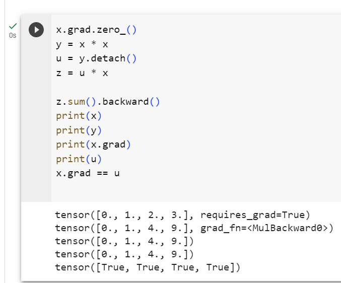
Note that while this procedure detaches y’s ancestors from the graph leading to z, the computational graph leading to y persists and thus we can calculate the gradient of y with respect to x.
이 절차가 z로 이어지는 그래프에서 y의 조상을 분리하는 동안 y로 이어지는 계산 그래프는 지속되므로 x에 대한 y의 기울기를 계산할 수 있습니다.
x.grad.zero_()
y.sum().backward()
x.grad == 2 * x
이 코드는 PyTorch를 사용하여 그래디언트(미분)를 계산하는 예제입니다. 아래에서 코드를 한 줄씩 설명하겠습니다.
x.grad는 x에 대한 그래디언트(미분)를 나타내는 PyTorch 텐서입니다. 이 코드는 이전에 계산된 그래디언트를 지우고 새로운 그래디언트를 계산할 준비를 합니다. zero_() 메서드는 그래디언트를 모두 0으로 초기화합니다.
y의 모든 원소의 합에 대한 그래디언트를 계산합니다. 이러한 그래디언트 계산은 역전파(backpropagation)를 통해 수행됩니다. 여기서 y는 x의 제곱인 텐서입니다.
- 이 코드는 x.grad와 2 * x를 비교합니다. x.grad는 y.sum()에 대한 그래디언트이며, 이것은 y가 x의 제곱이므로 2 * x입니다. 따라서 이 비교는 True를 반환합니다.
즉, x.grad는 y를 x로 미분한 결과이며, 이는 y가 2 * x의 형태를 가지는 관계를 반영합니다. 이것은 연쇄 법칙(Chain Rule)을 통해 계산되며, y가 x에 대한 제곱 함수인 경우 그래디언트는 2 * x가 됩니다.
tensor([True, True, True, True])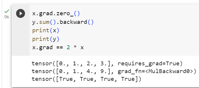
2.5.4. Gradients and Python Control Flow
So far we reviewed cases where the path from input to output was well defined via a function such as z = x * x * x. Programming offers us a lot more freedom in how we compute results. For instance, we can make them depend on auxiliary variables or condition choices on intermediate results. One benefit of using automatic differentiation is that even if building the computational graph of a function required passing through a maze of Python control flow (e.g., conditionals, loops, and arbitrary function calls), we can still calculate the gradient of the resulting variable. To illustrate this, consider the following code snippet where the number of iterations of the while loop and the evaluation of the if statement both depend on the value of the input a.
지금까지 우리는 z = x * x * x와 같은 함수를 통해 입력에서 출력까지의 경로가 잘 정의된 사례를 검토했습니다. 프로그래밍은 결과를 계산하는 방법에 있어 훨씬 더 많은 자유를 제공합니다. 예를 들어, 중간 결과에 대한 보조 변수나 조건 선택에 의존하도록 만들 수 있습니다. 자동 미분을 사용하면 미로 같은 Python 제어 흐름(예: 조건문, 루프 및 임의 함수 호출)을 통과해야 하는 함수의 계산 그래프를 작성하더라도 결과 변수의 기울기를 계속 계산할 수 있다는 이점이 있습니다. 이를 설명하기 위해 while 루프의 반복 횟수와 if 문의 평가가 모두 입력 a의 값에 따라 달라지는 다음 코드 조각을 고려해보세요.
def f(a):
    b = a * 2
    while b.norm() < 1000:
        b = b * 2
    if b.sum() > 0:
        c = b
    else:
        c = 100 * b
    return c
이 코드는 파이썬 함수 f(a)를 정의합니다. 이 함수는 입력으로 스칼라 텐서 a를 받아서 다음과 같은 작업을 수행합니다.
- b라는 새로운 변수를 생성하고 a에 2를 곱한 값을 할당합니다.
- b의 L2 노름(norm)이 1000보다 작을 때까지 b를 2배씩 계속해서 곱해갑니다. 이것은 b가 L2 노름이 1000보다 커질 때까지 반복하는 루프입니다.
- 만약 b의 원소들의 합이 0보다 크다면, c에 b를 할당합니다.
- 그렇지 않다면 (즉, b의 원소들의 합이 0 이하인 경우), c에 100을 곱한 b를 할당합니다.
- 최종적으로 c를 반환합니다.
이 함수는 입력 a를 사용하여 b를 계산하고, 이후에 b의 크기와 합을 고려하여 c를 정합니다. c의 값은 a와 b에 따라 다르며, 함수의 결과로 반환됩니다.
Below, we call this function, passing in a random value, as input. Since the input is a random variable, we do not know what form the computational graph will take. However, whenever we execute f(a) on a specific input, we realize a specific computational graph and can subsequently run backward.
아래에서는 이 함수를 호출하여 임의의 값을 입력으로 전달합니다. 입력이 랜덤 변수이기 때문에 계산 그래프가 어떤 형태를 취할지 알 수 없습니다. 그러나 특정 입력에 대해 f(a)를 실행할 때마다 특정 계산 그래프를 실현하고 이후에 역방향으로 실행할 수 있습니다.
a = torch.randn(size=(), requires_grad=True)
d = f(a)
d.backward()
이 코드는 PyTorch를 사용하여 작성된 것으로 보이는 예제입니다. 코드는 다음과 같은 작업을 수행합니다:
- a라는 이름의 스칼라 텐서를 생성합니다. requires_grad=True 매개변수를 사용하여 a에 대한 경사도(gradient)가 계산되도록 설정합니다.
- 이전에 정의한 f(a) 함수를 호출하여 a를 입력으로 사용하고, 이를 d에 할당합니다.
- backward 메서드를 사용하여 d의 경사도를 계산합니다. 이것은 연쇄 법칙(chain rule)을 사용하여 d를 a에 대한 함수로 간주하고, d의 a에 대한 경사도를 계산합니다.
즉, 코드는 a에서 f(a)로의 계산 그래프를 구성하고, f(a)의 결과 d에 대한 a의 경사도를 계산합니다. 이렇게 하면 a.grad에 a에 대한 경사도가 저장됩니다.
Even though our function f is, for demonstration purposes, a bit contrived, its dependence on the input is quite simple: it is a linear function of a with piecewise defined scale. As such, f(a) / a is a vector of constant entries and, moreover, f(a) / a needs to match the gradient of f(a) with respect to a.
함수 f는 데모 목적으로 약간 인위적으로 만들어졌지만 입력에 대한 의존성은 매우 간단합니다. 부분적으로 정의된 스케일을 사용하는 a의 선형 함수입니다. 따라서 f(a) / a는 상수 항목으로 구성된 벡터이며 더욱이 f(a) / a는 a에 대한 f(a)의 기울기와 일치해야 합니다.
a.grad == d / a이 코드는 a.grad와 d를 a로 나눈 값인 d / a를 비교하여 결과를 확인합니다.
a.grad는 a에 대한 경사도(gradient)를 나타내며, 이 값은 .backward()를 호출하여 계산됩니다.
d는 f(a) 함수의 결과를 나타내는 변수입니다.
따라서, a.grad는 d를 a로 미분한 값이 됩니다. 코드는 이 계산된 경사도 a.grad와 d / a를 비교하여 두 값이 동일한지 확인합니다.
이 비교가 참인 경우, 이는 PyTorch의 자동 미분이 제대로 작동하고 있다는 것을 의미합니다. 즉, d를 a로 미분한 결과가 d / a와 일치한다는 것을 의미합니다.
tensor(True)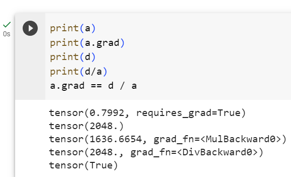
Dynamic control flow is very common in deep learning. For instance, when processing text, the computational graph depends on the length of the input. In these cases, automatic differentiation becomes vital for statistical modeling since it is impossible to compute the gradient a priori.
동적 제어 흐름은 딥러닝에서 매우 일반적입니다. 예를 들어 텍스트를 처리할 때 계산 그래프는 입력 길이에 따라 달라집니다. 이러한 경우 사전에 기울기를 계산하는 것이 불가능하기 때문에 통계 모델링에 자동 미분이 필수적입니다.
2.5.5. Discussion
You have now gotten a taste of the power of automatic differentiation. The development of libraries for calculating derivatives both automatically and efficiently has been a massive productivity booster for deep learning practitioners, liberating them so they can focus on less menial. Moreover, autograd lets us design massive models for which pen and paper gradient computations would be prohibitively time consuming. Interestingly, while we use autograd to optimize models (in a statistical sense) the optimization of autograd libraries themselves (in a computational sense) is a rich subject of vital interest to framework designers. Here, tools from compilers and graph manipulation are leveraged to compute results in the most expedient and memory-efficient manner.
이제 자동 미분의 힘을 맛보셨습니다. 도함수를 자동으로 효율적으로 계산하기 위한 라이브러리의 개발은 딥 러닝 실무자들의 생산성을 대폭 향상시켜 그들이 덜 천박한 일에 집중할 수 있도록 해방시켜 주었습니다. 게다가, autograd를 사용하면 펜과 종이의 그라디언트 계산에 엄청난 시간이 소요되는 대규모 모델을 설계할 수 있습니다. 흥미롭게도, 우리가 모델을 최적화하기 위해(통계적 의미에서) autograd를 사용하는 반면, autograd 라이브러리 자체의 최적화(계산적 의미에서)는 프레임워크 설계자들에게 매우 중요한 주제입니다. 여기서는 컴파일러 도구와 그래프 조작을 활용하여 가장 편리하고 메모리 효율적인 방식으로 결과를 계산합니다.
For now, try to remember these basics: (i) attach gradients to those variables with respect to which we desire derivatives; (ii) record the computation of the target value; (iii) execute the backpropagation function; and (iv) access the resulting gradient.
지금은 다음 기본 사항을 기억해 보십시오. (i) 도함수를 원하는 변수에 기울기를 적용합니다. (ii) 목표값의 계산을 기록하고; (iii) 역전파 기능을 실행합니다. (iv) 결과 그래디언트에 액세스합니다.
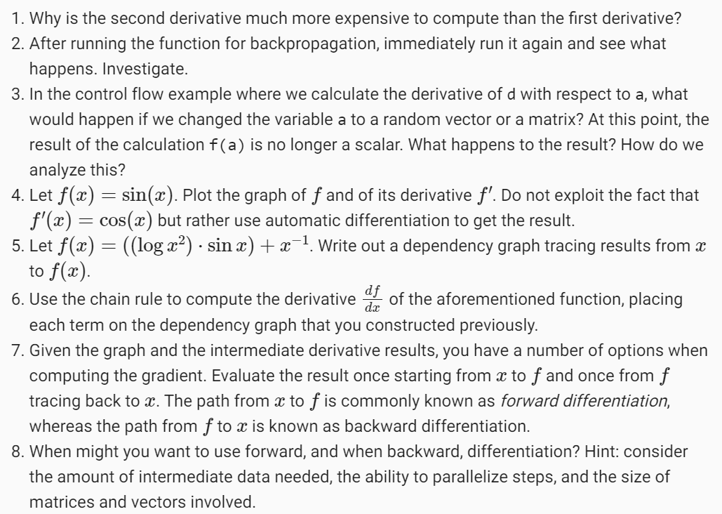
2.5.6. Exercises
'Dive into Deep Learning > D2L Preliminaries' 카테고리의 다른 글
| D2L - 2.7. Documentation (2) | 2023.10.14 |
|---|---|
| D2L - 2.6. Probability and Statistics (0) | 2023.10.14 |
| D2L - 2.4. Calculus : 미적분 (1) | 2023.10.12 |
| D2L - 2.3. Linear Algebra - 선형 대수학 (1) | 2023.10.11 |
| D2L - 2.2. Data Preprocessing (0) | 2023.10.09 |
| D2L - 2.1. Data Manipulation (0) | 2023.10.09 |
| D2L - 2. Preliminaries (0) | 2023.10.09 |