개발자로서 현장에서 일하면서 새로 접하는 기술들이나 알게된 정보 등을 정리하기 위한 블로그입니다. 운 좋게 미국에서 큰 회사들의 프로젝트에서 컬설턴트로 일하고 있어서 새로운 기술들을 접할 기회가 많이 있습니다. 미국의 IT 프로젝트에서 사용되는 툴들에 대해 많은 분들과 정보를 공유하고 싶습니다.
Before we worry about making our neural networks deep, it will be helpful to implement some shallow ones, for which the inputs connect directly to the outputs. This will prove important for a few reasons. First, rather than getting distracted by complicated architectures, we can focus on the basics of neural network training, including parametrizing the output layer, handling data, specifying a loss function, and training the model. Second, this class of shallow networks happens to comprise the set of linear models, which subsumes many classical methods of statistical prediction, including linear and softmax regression. Understanding these classical tools is pivotal because they are widely used in many contexts and we will often need to use them as baselines when justifying the use of fancier architectures. This chapter will focus narrowly on linear regression and the next one will extend our modeling repertoire by developing linear neural networks for classification.
신경망을 깊게 만드는 것에 대해 걱정하기 전에 입력이 출력에 직접 연결되는 얕은 신경망을 구현하는 것이 도움이 될 것입니다. 이는 몇 가지 이유로 중요할 것입니다. 첫째, 복잡한 아키텍처로 인해 산만해지기보다는 출력 레이어 매개변수화, 데이터 처리, 손실 함수 지정, 모델 훈련 등 신경망 훈련의 기본에 집중할 수 있습니다. 둘째, 이 얕은 네트워크 클래스는 선형 및 소프트맥스 회귀를 포함하여 많은 고전적인 통계 예측 방법을 포함하는 선형 모델 세트로 구성됩니다. 이러한 고전적인 도구는 다양한 상황에서 널리 사용되며 더 멋진 아키텍처의 사용을 정당화할 때 이를 기준으로 사용해야 하기 때문에 이를 이해하는 것이 매우 중요합니다. 이 장에서는 선형 회귀에 초점을 맞추고 다음 장에서는 분류를 위한선형 신경망을 개발하여 모델링 레퍼토리를 확장합니다.
3.1. Linear Regression (선형 회귀)
- Regression (회귀) : 주어진 데이터 포인트 x에 해당하는 실제 값으로 주어지는 타겟 y를 예측하는 과제.
예1) 주택가격, 주가, 기온, 판매량, 입원기간 예측 같은 연속된 값을 예측하는 문제
예2) 주택가격 책정 - 면적, years, 이전 매매가격, 위치 등의 training data set (training set) 가 필요함
- 주로 숫자 값을 예측하려 할 때 나타남.
- Regression 문제와 구별되는 것은 discrete (이산적인) classification (구분) 문제가 있음 (소속을 예측하는 문제)
Terminology ***
Training Dataset(Training set) : Target y 를 구하기 위해 제공된는 데이터 x들을 일컫는 말
Example (data point, instance, sample) : 한개의 데이터 포인트 x (row) . (하나의 집)
Label (Target) : 우리가 예측 하려는 것. (집의 판매 가격)
Features (Covariates): 예측의 기반이 되는 변수들.(Label을 예측하기 위해 사용된 값)
이후 나오는 예제는 PYTORCH를 사용할 것임.
PYTORCH 란?
PyTorch is an open-source deep learning framework that provides a flexible and dynamic approach to building and training neural networks. It is widely used in the field of artificial intelligence (AI) and has gained popularity due to its ease of use and efficient computation capabilities.
PyTorch는 유연하고 동적인 방식으로 신경망을 구축하고 훈련할 수 있는 오픈 소스 딥러닝 프레임워크입니다. 인공지능(AI) 분야에서 널리 사용되며 사용 편의성과 효율적인 연산 능력으로 인기를 얻고 있습니다.
Here are some key features of PyTorch:
PyTorch의 주요 특징은 다음과 같습니다:
Dynamic computation graph: PyTorch uses a dynamic computational graph, which allows you to define and modify the computation graph on the fly. This flexibility makes it easier to debug and experiment with different network architectures. 동적 계산 그래프: PyTorch는 동적 계산 그래프를 사용하여 계산 그래프를 실시간으로 정의하고 수정할 수 있습니다. 이 유연성은 디버깅 및 다양한 네트워크 아키텍처 실험에 유용합니다.
Automatic differentiation: PyTorch provides automatic differentiation, which means it can automatically compute gradients for you. Gradients are essential for optimizing neural networks using gradient descent-based algorithms such as backpropagation. The autograd package in PyTorch enables automatic differentiation, making it easier to train models. 자동 미분: PyTorch는 자동 미분을 제공하여 자동으로 그래디언트를 계산할 수 있습니다. 그래디언트는 역전파와 같은 그래디언트 하강 기반 알고리즘을 사용하여 신경망을 최적화하는 데 필수적입니다. PyTorch의 autograd 패키지는 자동 미분을 가능하게 하며, 모델 훈련을 쉽게 할 수 있습니다.
GPU acceleration: PyTorch supports seamless GPU acceleration for faster training and inference. It leverages the power of Graphics Processing Units (GPUs) to perform parallel computations, which significantly speeds up the training process for deep learning models. GPU 가속화: PyTorch는 빠른 훈련과 추론을 위해 매끄러운 GPU 가속을 지원합니다. GPU의 파워를 활용하여 병렬 계산을 수행하여 딥러닝 모델의 훈련 과정을 크게 가속화할 수 있습니다.
Dynamic neural networks: With PyTorch, you can build dynamic neural networks that can change their architecture during runtime. This capability allows for the creation of complex models with variable input sizes, recurrent connections, and conditional branching. 동적 신경망: PyTorch를 사용하면 런타임 중에 아키텍처를 변경할 수 있는 동적 신경망을 구축할 수 있습니다. 이 기능을 사용하여 변수 크기의 입력, 순환 연결 및 조건 분기를 포함한 복잡한 모델을 만들 수 있습니다.
Rich ecosystem and community support: PyTorch has a vibrant community and provides extensive documentation, tutorials, and pre-trained models. It also integrates well with other popular libraries and frameworks, such as NumPy, SciPy, and scikit-learn. 다양한 생태계와 커뮤니티 지원: PyTorch는 활발한 커뮤니티를 가지고 있으며, 상세한 문서, 튜토리얼 및 사전 훈련된 모델을 제공합니다. 또한 NumPy, SciPy, scikit-learn과 같은 인기있는 라이브러리와 프레임워크와 잘 통합됩니다.
Overall, PyTorch offers a user-friendly and intuitive interface for deep learning research and development. It provides a solid foundation for implementing various machine learning algorithms, including linear regression, convolutional neural networks (CNNs), recurrent neural networks (RNNs), and more.
전반적으로 PyTorch는 딥러닝 연구 및 개발에 사용자 친화적이고 직관적인 인터페이스를 제공합니다. 선형 회귀, 합성곱 신경망(CNN), 순환 신경망(RNN) 등 다양한 머신러닝 알고리즘을 구현하는 데 견고한 기반을 제공합니다.
첫번째 예제
%matplotlib inline
import math
import time
import numpy as np
import torch
from d2l import torch as d2l
코드 설명
The code snippet you provided imports necessary libraries and modules for working with PyTorch and the "d2l" library, which is a companion library for the book "Dive into Deep Learning."
제공한 코드 조각은 PyTorch 및 "Dive into Deep Learning"의 동반 라이브러리인 "d2l"을 사용하기 위한 필수 라이브러리 및 모듈을 가져옵니다.
Here is a breakdown of the code:
아래는 코드의 세부 내용을 설명한 것입니다:
%matplotlib inline: This is a Jupyter Notebook magic command that enables the inline plotting of graphs within the notebook. %matplotlib inline: 이는 Jupyter Notebook의 매직 명령어로, 노트북 내에서 그래프를 인라인으로 표시할 수 있도록 합니다.
import math: This imports the math module, which provides mathematical functions and constants. import math: math 모듈을 가져옵니다. 이 모듈은 수학 함수와 상수를 제공합니다.
import time: This imports the time module, which allows you to measure and control the execution time of your code. import time: time 모듈을 가져옵니다. 이 모듈은 코드의 실행 시간을 측정하고 제어하는 기능을 제공합니다.
import numpy as np: This imports the NumPy library, which provides support for efficient numerical computations and arrays. import numpy as np: NumPy 라이브러리를 가져옵니다. 이 라이브러리는 효율적인 수치 계산과 배열에 대한 지원 기능을 제공합니다.
import torch: This imports the PyTorch library, which is the main focus of the code. It provides functionalities for building, training, and evaluating neural networks. import torch: PyTorch 라이브러리를 가져옵니다. 이 코드의 주요 대상입니다. PyTorch는 신경망을 구축하고 훈련하며 평가하는 데 필요한 기능을 제공합니다.
from d2l import torch as d2l: This imports the d2l module from the "d2l" library. The "d2l" library is a collection of utility functions and custom layers specifically designed to accompany the book "Dive into Deep Learning." It provides convenient functions and utilities for working with PyTorch. from d2l import torch as d2l: "d2l" 라이브러리의 d2l 모듈을 가져옵니다. "d2l" 라이브러리는 "Dive into Deep Learning" 책과 함께 사용하기 위해 특별히 설계된 유틸리티 함수와 사용자 정의 레이어의 모음입니다. PyTorch와 함께 사용하기 위한 편리한 함수와 유틸리티를 제공합니다.
By executing this code, you ensure that the necessary libraries and modules are imported and available for use in the subsequent code snippets.
이 코드를 실행함으로써 필요한 라이브러리와 모듈이 가져와져서 이후의 코드 조각에서 사용할 수 있게 됩니다.
코드 실행 결과
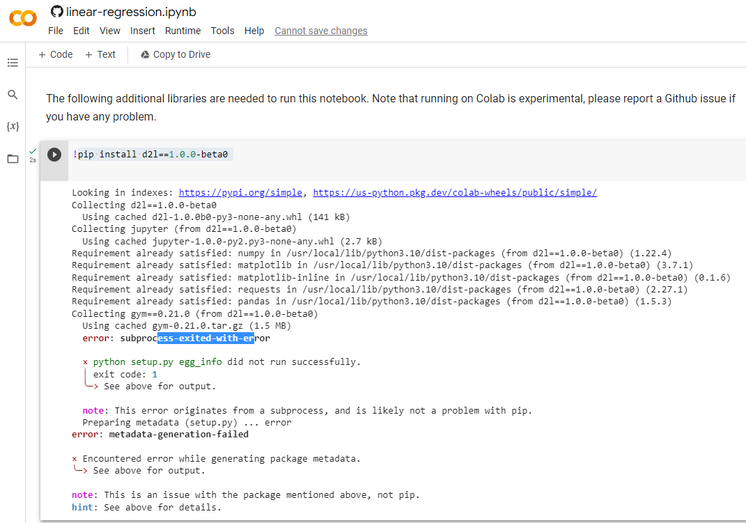
pip install d2l==1.0.0-beta0
Looking in indexes: https://pypi.org/simple, https://us-python.pkg.dev/colab-wheels/public/simple/
Collecting d2l==1.0.0-beta0
  Downloading d2l-1.0.0b0-py3-none-any.whl (141 kB)
     ━━━━━━━━━━━━━━━━━━━━━━━━━━━━━━━━━━━━━━━ 141.6/141.6 kB 7.7 MB/s eta 0:00:00
Collecting jupyter (from d2l==1.0.0-beta0)
  Downloading jupyter-1.0.0-py2.py3-none-any.whl (2.7 kB)
Requirement already satisfied: numpy in /usr/local/lib/python3.10/dist-packages (from d2l==1.0.0-beta0) (1.22.4)
Requirement already satisfied: matplotlib in /usr/local/lib/python3.10/dist-packages (from d2l==1.0.0-beta0) (3.7.1)
Requirement already satisfied: matplotlib-inline in /usr/local/lib/python3.10/dist-packages (from d2l==1.0.0-beta0) (0.1.6)
Requirement already satisfied: requests in /usr/local/lib/python3.10/dist-packages (from d2l==1.0.0-beta0) (2.27.1)
Requirement already satisfied: pandas in /usr/local/lib/python3.10/dist-packages (from d2l==1.0.0-beta0) (1.5.3)
Collecting gym==0.21.0 (from d2l==1.0.0-beta0)
  Downloading gym-0.21.0.tar.gz (1.5 MB)
     ━━━━━━━━━━━━━━━━━━━━━━━━━━━━━━━━━━━━━━━━ 1.5/1.5 MB 48.4 MB/s eta 0:00:00
  error: subprocess-exited-with-error

  × python setup.py egg_info did not run successfully.
  │ exit code: 1
  ╰─> See above for output.

  note: This error originates from a subprocess, and is likely not a problem with pip.
  Preparing metadata (setup.py) ... error
error: metadata-generation-failed

× Encountered error while generating package metadata.
╰─> See above for output.

note: This is an issue with the package mentioned above, not pip.
%matplotlib inline
import math
import time
import numpy as np
import torch
from d2l import torch as d2l
ModuleNotFoundError Traceback (most recent call last)
<ipython-input-3-7a344dafd5da> in <cell line: 6>()
4 import numpy as np
5 import torch
----> 6 from d2l import torch as d2l
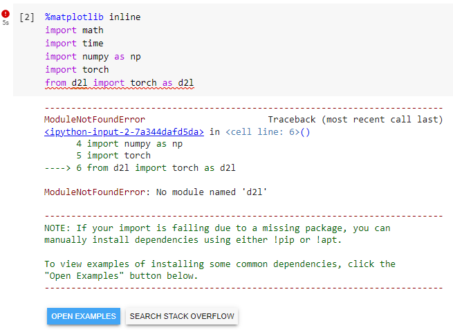
ModuleNotFoundError: No module named 'd2l'
---------------------------------------------------------------------------
NOTE: If your import is failing due to a missing package, you can
manually install dependencies using either !pip or !apt.
To view examples of installing some common dependencies, click the
"Open Examples" button below.
---------------------------------------------------------------------------
==> Local에서 시도해도 같은 결과임.
3.1.1. Basics
Linear regressionis both the simplest and most popular among the standard tools for tackling regression problems. Dating back to the dawn of the 19th century(Gauss, 1809,Legendre, 1805), linear regression flows from a few simple assumptions.
선형 회귀는 회귀 문제를 해결하기 위한 표준 도구 중에서 가장 간단하고 널리 사용됩니다. 19세기 초(Gauss, 1809, Legendre, 1805)로 거슬러 올라가는 선형 회귀는 몇 가지 간단한 가정에서 시작되었습니다.
First, we assume that the relationship between featuresxand targetyis approximately linear, i.e., that the conditional meanE[Y∣X=x]can be expressed as a weighted sum of the featuresx. This setup allows that the target value may still deviate from its expected value on account of observation noise.
먼저, 특징 features x와 목표 target y 사이의 관계가 대략 선형 linear 이라고 가정합니다. 즉, 조건부 평균 conditional mean E[Y∣X=x]는 특징 x의 가중 합으로 표현될 수 있습니다. 이 설정을 사용하면 관찰 노이즈로 인해 목표 값이 여전히 예상 값에서 벗어날 수 있습니다.
Next, we can impose the assumption that any such noise is well behaved, following a Gaussian distribution. Typically, we will usento denote the number of examples in our dataset. We use superscripts to enumerate samples and targets, and subscripts to index coordinates. More concretely,x**(i)denotes thei thsample andxj(i)denotes itsjthcoordinate.
다음으로, 가우스 분포에 따라 그러한 잡음이 잘 동작한다는 가정을 부과할 수 있습니다. 일반적으로 데이터 세트의 예제 수를 나타내기 위해 n을 사용합니다. 샘플과 타겟을 열거하기 위해 위 첨자를 사용하고, 인덱스 좌표에 아래 첨자를 사용합니다. 보다 구체적으로 x**(i)는 i번째 샘플을 나타내고 xj(i)는 해당 샘플의 j번째 좌표를 나타냅니다.
- Linear Regression은 가장 간단하면서도 가장 널리 이용되는 Regression 문제들을 해결하기 위한 표준 도구
- Linear Regression은 몇가지 간단한 가정들이 전제 된다.
* features x 와 target y의 관계는 선형적이라고 가정한다.
* 조건부 평균 E[Y|X=x] 는 features x 의 가중합 (weighted sum)으로 표현될 수 있음
* 이 설정을 사용하면 관찰 노이즈로 인해 target 값이 expected 값에서 벗어날 수 있음
* Gaussian distribution (정규분포)을 따르면 그러한 노이즈들이 올바르게 작동한는 가정을 할 수 있음
* n을 사용하여 data set의 examples의 수를 나타낼 것임
* 윗첨자 (superscript)를 사용하여 samples와 target을 표현할 것임
* 아랫첨자(subscript)를 사용하여 인덱스 좌표를 나타내는데 사용할 것임
x(i) : 이것은 i 번째 sample임을 나타냄
x(i)j : 이것은 j번째 coordinate 임을 나타냄
Linear algebra (선형 대수학) 에서 선형성 (Linear) 란?
함수f에 대하여,
1.가산성 (Additivity): 임의의x,y,에 대하여,f(x+y)=f(x)+f(y)
2.동치성 (Homogeneity): 임의의 수α에 대하여,f(αx)=αf(x)
위 두 성질이 항상 성립할 때 함수f는 선형적이라고 한다.
조건부 평균 E[Y|X=x] 에 대하여.
In linear algebra, the notation E[Y|X=x] represents the conditional expectation of a random variable Y given that another random variable X takes on a specific value x. It is a concept from probability theory that relates to the expected value of a random variable under a specific condition.
선형 대수에서 E[Y|X=x] 표기는 조건부 기댓값을 의미합니다. 여기서 Y는 다른 랜덤 변수 X가 특정 값 x를 가질 때의 조건부 기댓값입니다. 이는 확률 이론에서 사용되는 개념으로, 특정 조건 하에서 랜덤 변수의 기댓값과 관련이 있습니다.
To break it down:
자세히 설명하면 다음과 같습니다:
E[Y|X] denotes the conditional expectation of Y given X.
E[Y|X]는 X가 주어졌을 때 Y의 조건부 기댓값을 나타냅니다.
x represents a specific value that X can take on.
x는 X가 가질 수 있는 특정 값입니다.
The expression E[Y|X=x] indicates that we are interested in the expected value of Y when X is fixed at the value x. It represents the average or expected value of Y when the condition X=x is satisfied.
표현식 E[Y|X=x]은 X가 값 x로 고정되었을 때의 Y의 기댓값을 의미합니다. 이는 조건 X=x가 만족되는 경우 Y의 평균값 또는 기댓값을 나타냅니다.
Conditional expectation allows us to analyze the relationship between two random variables and understand how the value of one variable influences the expected value of another variable when a certain condition is met.
조건부 기댓값은 두 개의 랜덤 변수 간의 관계를 분석하고, 특정 조건이 충족되었을 때 한 변수의 값이 다른 변수의 기댓값에 어떤 영향을 미치는지 이해하는 데 도움을 줍니다.
E[Y∣X=x] 란?
수식E[Y∣X=x]은 랜덤 변수Y의 조건부 기대값을 나타냅니다. 여기에 나오는 표기법에 대한 설명은 다음과 같습니다:
E: 기대값을 나타내며, 이는 확률 분포의 중심 또는 평균을 나타냅니다.
Y: 기대값을 찾고자 하는 랜덤 변수입니다.
∣∣: 수직 막대는 "주어진" 또는 "조건부"를 나타냅니다.
X=x: 이것은 랜덤 변수X가 특정 값x를 가질 때의 시나리오를 나타냅니다.
따라서E[Y∣X=x]는 "X가 특정 값x일 때의Y의 조건부 기대값"으로 해석됩니다. 이는 우리가X가 특정 값x를 가질 때Y가 가질 평균 값으로 생각할 수 있습니다.
조건부 기대값에 대한 이 수식은 주로 확률 이론과 통계에서 사용됩니다. 이 개념은 다른 랜덤 변수의 값에 조건을 걸었을 때, 기대값이 어떻게 변하는지 이해하는 데 중요합니다. 이는 랜덤 변수 간의 관계를 모델링하고 분석하는 데 필수적인 도구입니다.
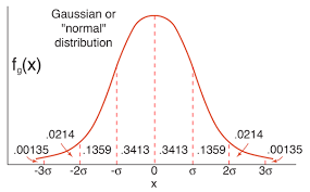
What is Gaussian distribution?
The Gaussian distribution, also known as the normal distribution or bell curve, is a continuous probability distribution that is widely used in statistics and probability theory. It is characterized by its symmetric, bell-shaped curve when plotted on a graph.
가우시안 분포는 확률론과 통계학에서 널리 사용되는 연속형 확률 분포로, 정규 분포 또는 종모양 곡선으로도 알려져 있습니다. 그래프로 그릴 때는 대칭적이고 종 모양의 곡선으로 특징화됩니다.
Here are some key properties and characteristics of the Gaussian distribution:
가우시안 분포의 주요 특성과 특징은 다음과 같습니다:
Shape: The Gaussian distribution has a symmetric shape, with the peak of the curve occurring at the mean (average) value. The curve is bell-shaped and tapers off gradually as it extends towards positive and negative infinity. 형태: 가우시안 분포는 대칭적인 모양을 가지며, 곡선의 정점은 평균값(평균)에 해당합니다. 곡선은 종 모양이며, 양의 무한대와 음의 무한대로 갈수록 서서히 감소합니다.
Central Limit Theorem: The Gaussian distribution plays a fundamental role in the Central Limit Theorem, which states that the sum or average of a large number of independent and identically distributed random variables tends to follow a Gaussian distribution, regardless of the underlying distribution of the individual variables. 중심극한정리: 가우시안 분포는 중심극한정리에서 중요한 역할을 합니다. 중심극한정리는 독립적이고 동일하게 분포된 많은 수의 확률 변수의 합 또는 평균이 기본 분포와 상관없이 가우시안 분포를 따른다는 것을 말합니다.
Parameters: The Gaussian distribution is defined by two parameters: the mean (μ) and the standard deviation (σ). The mean represents the center of the distribution, while the standard deviation determines the spread or dispersion of the data. The variance (σ^2) is the square of the standard deviation. 파라미터: 가우시안 분포는 평균(μ)과 표준편차(σ) 두 가지 파라미터로 정의됩니다. 평균은 분포의 중심을 나타내고, 표준편차는 데이터의 분산이나 퍼짐 정도를 결정합니다. 분산(σ^2)은 표준편차의 제곱입니다.
Probability Density Function (PDF): The probability density function of the Gaussian distribution is given by the formula:where e is the base of the natural logarithm. 확률 밀도 함수 (PDF): 가우시안 분포의 확률 밀도 함수는 다음 수식으로 주어집니다:여기서 e는 자연로그의 밑을 나타냅니다. f(x) = (1 / √(2πσ^2)) * e^(-(x-μ)^2 / (2σ^2)) 여기서 e는 자연로그의 밑을 나타냅니다.
Empirical Rule: The Gaussian distribution follows the Empirical Rule (also known as the 68-95-99.7 rule), which states that approximately 68% of the data falls within one standard deviation of the mean, about 95% falls within two standard deviations, and roughly 99.7% falls within three standard deviations. 경험적 법칙: 가우시안 분포는 경험적 법칙(또는 68-95-99.7 법칙)을 따릅니다. 이 법칙에 따르면 대략 68%의 데이터가 평균에서 표준편차의 범위 내에 있으며, 약 95%는 평균에서 2배 표준편차의 범위 내에 있으며, 대략 99.7%는 평균에서 3배 표준편차의 범위 내에 있습니다.
Applications: The Gaussian distribution is commonly used in various fields, including statistics, physics, finance, and engineering. It serves as an important assumption in many statistical models and methods, and it provides a foundation for performing statistical inference and hypothesis testing. 응용: 가우시안 분포는 통계, 물리학, 금융, 공학 등 다양한 분야에서 널리 사용됩니다. 많은 통계 모델과 방법에서 중요한 가정이 되며, 통계적 추론과 가설 검정을 수행하는 데 기초를 제공합니다.
The Gaussian distribution is widely studied and utilized due to its mathematical tractability and its prevalence in natural and social phenomena. It serves as a useful tool for describing and analyzing random variables and their associated probabilities.
가우시안 분포는 수학적으로 다루기 쉽고 자연적이며 사회적 현상에서 많이 나타나기 때문에 널리 연구되고 활용됩니다. 확률 변수와 관련된 확률을 기술하고 분석하는 유용한 도구로 사용됩니다.
3.1.1.1 Model
At the heart of every solution is a model that describes how features can be transformed into an estimate of the target. The assumption of linearity means that the expected value of the target (price) can be expressed as a weighted sum of the features (area and age):
모든 솔루션의 중심에는 기능을 목표 추정치로 변환하는 방법을 설명하는 모델이 있습니다. 선형성 가정은 목표(가격)의 기대값이 특성(면적 및 연령)의 가중합으로 표현될 수 있음을 의미합니다.
- features를 가지고 어떻게 target을 estimate하는지를 설명하는 Model은 모든 solution의 핵심이다.
- linear means의 가정은 target (가격)의 기대값이 features (면적, 연령)의 가중합계 (weighted sum)으로 표현됨을 의미
price = warea * area + wage * age + b (3.1.1)
warea 와 wage 를 weights (가중치) 라고 하고 b는 bias (of offset or intercept)라고 한다.
weights (가중치)는 prediction(예측)에 대한 각 feature의 영향을 결정함
bias는 모든 features가 0일 때 estimate ((여기서는 price) 값을 결정함
Herew areaandw ageare calledweights, andbis called abias(oroffsetorintercept). The weights determine the influence of each feature on our prediction. The bias determines the value of the estimate when all features are zero. Even though we will never see any newly-built homes with precisely zero area, we still need the bias because it allows us to express all linear functions of our features (rather than restricting us to lines that pass through the origin). Strictly speaking,(3.1.1)is anaffine transformationof input features, which is characterized by alinear transformationof features via a weighted sum, combined with atranslationvia the added bias. Given a dataset, our goal is to choose the weightswand the biasbthat, on average, make our model’s predictions fit the true prices observed in the data as closely as possible.
여기서 w area 과 w age 을 가중치라고 하고 b를 편향(또는 오프셋 또는 절편)이라고 합니다. 가중치는 예측에 대한 각 특성의 영향을 결정합니다. 편향은 모든 특성이 0일 때 추정값을 결정합니다. 면적이 정확히 0인 새로 지어진 주택을 결코 볼 수 없더라도 바이어스를 사용하면 (원점을 통과하는 선으로 제한하지 않고) 기능의 모든 선형 기능을 표현할 수 있기 때문에 여전히 바이어스가 필요합니다. 엄밀히 말하면, (3.1.1)은 입력 특성의 아핀 변환으로, 추가된 편향을 통한 변환과 결합된 가중 합을 통한 특성의 선형 변환을 특징으로 합니다. 데이터 세트가 주어지면 우리의 목표는 평균적으로 모델의 예측이 데이터에서 관찰된 실제 가격과 최대한 일치하도록 가중치 w와 편향 b를 선택하는 것입니다.
엄밀히 말하면 3.1.1은 가중합계, 추가적인 bias를 통해 translation되고 combine된 것들을 통해 features의 linear transformation에 의해 특정되어진 입력 features의 affine transformation이다.
Affine transformation 이란?
An affine transformation refers to a geometric transformation that preserves parallel lines and ratios of distances. It is a type of transformation commonly used in computer graphics, computer vision, and image processing.
어파인 변환(affine transformation)은 평행선과 거리 비율을 보존하는 기하학적 변환을 의미합니다. 이는 컴퓨터 그래픽스, 컴퓨터 비전, 이미지 처리 등에서 자주 사용되는 변환 유형입니다.
Key characteristics of affine transformations are as follows:
어파인 변환의 주요 특징은 다음과 같습니다:
Line Preservation: Affine transformations maintain the parallelism of lines. This means that if two lines are parallel before the transformation, they will remain parallel after the transformation. 선 보존: 어파인 변환은 선의 평행성을 유지합니다. 즉, 변환 전에 평행한 두 선은 변환 후에도 평행한 상태를 유지합니다.
Ratio Preservation: Affine transformations preserve the ratio of distances along parallel lines. This property ensures that objects' shapes are preserved during the transformation. 비율 보존: 어파인 변환은 평행한 선 상의 거리 비율을 보존합니다. 이 속성은 변환 중에 객체의 형태를 보존합니다.
Combination of Translation, Rotation, Scaling, and Shearing: Affine transformations can be represented as a combination of translation (shifting), rotation (rotation around a point), scaling (resizing), and shearing (distorting in a non-uniform manner) operations. 이동, 회전, 스케일링, 기울임 변환의 조합: 어파인 변환은 이동(이동), 회전(특정 점을 중심으로 회전), 스케일링(크기 조정) 및 기울임(비등방적 왜곡) 연산의 조합으로 나타낼 수 있습니다.
Linearity: Affine transformations are linear transformations, which means they preserve the properties of linearity such as preserving the origin and vector addition. 선형성: 어파인 변환은 선형 변환으로, 원점과 벡터 덧셈 등 선형성의 속성을 보존합니다.
Matrix Representation: Affine transformations can be represented by a matrix multiplication. The transformation matrix includes parameters for translation, rotation, scaling, and shearing operations. 행렬 표현: 어파인 변환은 행렬 곱셈으로 표현될 수 있습니다. 변환 행렬에는 이동, 회전, 스케일링 및 기울임 연산에 대한 매개변수가 포함됩니다.
Applications of affine transformations include:
어파인 변환의 응용분야는 다음과 같습니다:
Computer Graphics: Affine transformations are used to render 2D and 3D graphics, such as transforming and projecting objects onto a screen or changing their size and position.
컴퓨터 그래픽스: 어파인 변환은 2D 및 3D 그래픽을 렌더링하는 데 사용되며, 객체를 화면에 투영하거나 크기와 위치를 변경하는 등의 작업에 활용됩니다.
Image Processing: Affine transformations are employed to perform operations such as scaling, rotating, and shearing images.
이미지 처리: 어파인 변환은 이미지의 크기 조정, 회전, 기울임 등을 수행하는 데 사용됩니다.
Computer Vision: Affine transformations play a role in tasks like object recognition, image registration, and feature extraction.
컴퓨터 비전: 어파인 변환은 객체 인식, 이미지 등록, 특징 추출 등의 작업에서 사용됩니다.
Geometric Modeling: Affine transformations are used to transform and manipulate geometric shapes in modeling applications.
기하 모델링: 어파인 변환은 모델링 애플리케이션에서 기하학적인 형상을 변환하고 조작하는 데 사용됩니다.
Overall, affine transformations provide a versatile and fundamental tool for manipulating and analyzing geometric objects in various fields.
전반적으로 어파인 변환은 다양한 분야에서 기하 객체를 조작하고 분석하는 다재다능하고 기본적인 도구를 제공합니다.
An image of a fern-likefractal(Barnsley's fern) that exhibits affineself-similarity. Each of the leaves of the fern is related to each other leaf by an affine transformation. For instance, the red leaf can be transformed into both the dark blue leaf and any of the light blue leaves by a combination of reflection, rotation, scaling, and translation.
***우리의 목표는 주어진 dataset에서 weight w와 bias b를 선택하는 겁니다. *** (항목마다 가중치를 얼마나 주고 bias를 얼마나 주어야 제대로 된 target을 얻을 수 있는가?) 그럼으로서 평균적으로 우리의 모델의 예측이 데이터에서 관찰된 실제 가격과 최대한 가까이 가도록 하는 겁니다.
In disciplines where it is common to focus on datasets with just a few features, explicitly expressing models long-form, as in(3.1.1), is common. In machine learning, we usually work with high-dimensional datasets, where it is more convenient to employ compact linear algebra notation. When our inputs consist ofdfeatures, we can assign each an index (between1and d ) and express our prediction ŷ (in general the “hat” symbol denotes an estimate) as
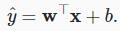
몇 가지 기능만 포함된 데이터 세트에 초점을 맞추는 것이 일반적인 분야에서는 (3.1.1)에서와 같이 모델을 긴 형식으로 명시적으로 표현하는 것이 일반적입니다. 기계 학습에서는 일반적으로 고차원 데이터 세트를 사용하여 압축 선형 대수 표기법을 사용하는 것이 더 편리합니다. 입력이 d개의 특징으로 구성되면 각각에 인덱스(1과 d 사이)를 할당하고 예측 ŷ(일반적으로 hat- symbol 는 추정치를 나타냄)를 다음과 같이 표현할 수 있습니다.
기계 학습에서는 흔히 ***다차원 데이터세트 (high-dimensional datasets) ***를 다룹니다.
예를 들어 입력값이 d 개의 features로 구성돼 있고 각각을 1에서 d 까지의 인덱스로 각각 할당할 수 있습니다.
여기서 우리의 prediction은 ŷ로 표기합니다. (일반적으로 ^ -hat- symbol은 estimate를 나타냄)
ŷ = w1x1 ... + wdxd + b. (3.1.2)
모든 features들과 weights들이 아래 vector일 경우
Collecting all features into a vectorx∈R**dand all weights into a vectorw∈R*d, we can express our model compactly via the dot product betweenwandx:
모든 특징을 벡터 x∈R**d로 수집하고 모든 가중치를 벡터 w∈R*d로 수집하면 w와 x 사이의 내적을 통해 모델을 간결하게 표현할 수 있습니다.
우리는 w와 x사이의 dot product를 통해 우리의 모델을 다음과 같이 표현할 수 있습니다.
(3.1.3)
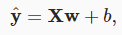
In(3.1.3), the vectorxcorresponds to the features of a single example. We will often find it convenient to refer to features of our entire dataset ofnexamples via thedesign matrixX∈R**n×d. Here,Xcontains one row for every example and one column for every feature. For a collection of featuresX, the predictions ŷ ∈R**ncan be expressed via the matrix–vector product:
(3.1.3)에서 벡터 x는 단일 예의 특징에 해당합니다. 우리는 설계 행렬 X∈R**n×d를 통해 n개의 예제로 구성된 전체 데이터 세트의 특징을 참조하는 것이 편리하다는 것을 종종 알게 될 것입니다. 여기서 X에는 모든 예에 대해 하나의 행과 모든 기능에 대해 하나의 열이 포함됩니다. 특성 X 모음의 경우 예측 ŷ ∈R**n은 행렬-벡터 곱을 통해 표현될 수 있습니다.
여기서 vector(벡터) x는 단일 예제의 특징 입니다.
Design matrix
위 디자인 매트릭스를 통해 n개의 examples로 구성된 전체 dataset의 features들을 참조하면 편리합니다.
여기서 X는 모든 example에 대한 하나의 row와 모든 feature에 대한 하나의 column을 포함합니다.
features X의 collection의 경우 matrix-vector product를 통해 아래 predictions로 표현될 수 있습니다.
:
(3.1.4)
training dataset X와 이에 해당하는 labels y는 주어진 features들입니다.
*** linear regression의 목표는 weight vector w와 bias term b를 찾는 것입니다. ***
이는 X와 동일한 분포로부터 sampled된 새로운 data example,의 주어진 features 을 기반으로 찾게 됩니다.
새로운 example의 label 은 낮은 오류로 예측 될 것입니다.
where broadcasting (Section 2.1.4) is applied during the summation. Given features of a training datasetXand corresponding (known) labelsy, the goal of linear regression is to find the weight vectorwand the bias termbsuch that, given features of a new data example sampled from the same distribution asX, the new example’s label will (in expectation) be predicted with the smallest error.
여기서는 합산 중에 브로드캐스팅(섹션 2.1.4)이 적용됩니다. 훈련 데이터세트 X의 특징과 해당(알려진) 라벨 y가 주어지면 선형 회귀의 목표는 X와 동일한 분포에서 샘플링된 새로운 데이터 예제의 주어진 특징이 다음과 같이 되도록 가중치 벡터 w와 편향 항 b를 찾는 것입니다. 새 예제의 레이블은 (예상대로) 가장 작은 오류로 예측됩니다.
Even if we believe that the best model for predictingygivenxis linear, we would not expect to find a real-world dataset ofnexamples wherey**(i)exactly equalsw⊤x**(i)+bfor all1≤i≤n. For example, whatever instruments we use to observe the featuresXand labelsy, there might be a small amount of measurement error. Thus, even when we are confident that the underlying relationship is linear, we will incorporate a noise term to account for such errors.
x가 주어졌을 때 y를 예측하는 가장 좋은 모델이 선형이라고 믿는다고 해도, y**(i)가 w⊤x**(i)+b와 정확히 일치하는 n개 사례의 실제 데이터 세트를 찾을 수는 없을 것입니다. 모두 1≤i≤n입니다. 예를 들어, 특징 X와 라벨 y를 관찰하기 위해 어떤 도구를 사용하든 약간의 측정 오류가 있을 수 있습니다. 따라서 기본 관계가 선형이라고 확신하는 경우에도 이러한 오류를 설명하기 위해 노이즈 항을 포함합니다.
Before we can go about searching for the bestparameters(ormodel parameters)wandb, we will need two more things: (i) a measure of the quality of some given model; and (ii) a procedure for updating the model to improve its quality.
최상의 매개변수(또는 모델 매개변수) w와 b를 검색하기 전에 두 가지가 더 필요합니다. (i) 특정 모델의 품질을 측정하는 것; (ii) 모델의 품질을 개선하기 위해 모델을 업데이트하는 절차.
주어진 x로 y를 예측하기 위한 가장 최적의 모델이 linear라고 믿는다고 해도, 우리는 1 <= i <= n에 대해 y(i)가 wTx(i)+b 와 정확히 같은 n examples의 실제 데이터 세트를 찾을 것이라고 기대하지는 않습니다.
예를 들어 features X와 labels Y를 관찰하는데 어떤 instruments를 사용하던 약간의 측정 오류는 있을 수 있습니다.
주택 가격의 경우 일반적으로 age가 더해 질 수록 가격이 하락하지만 역사적인 가치가 있는 경우 age가 더해 질 수록 가격이 더 올라갈 수도 있습니다.
그러므로 기본적으로 관계가 linear라고 확신해도 그러한 에러들을 설명하기 위해 noise term을 같이 사용합니다.
***
best parameters (or model parameters) w 와 b를 searching 하기 전에 우리는 다음의 두가지를 필요로 합니다.
1) 주어진 모델에 대한 품질 측정
2) 품질을 개선하기 위해 모델을 업데이트 하는 절차
***
3.1.1.2 Loss Function
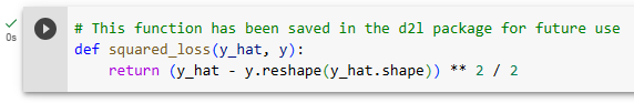
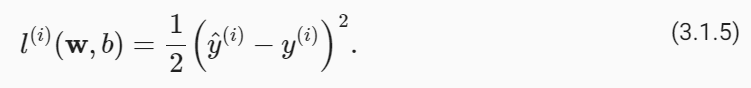
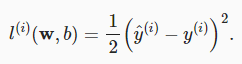
Naturally, fitting our model to the data requires that we agree on some measure offitness(or, equivalently, ofunfitness).Loss functionsquantify the distance between therealandpredictedvalues of the target. The loss will usually be a nonnegative number where smaller values are better and perfect predictions incur a loss of 0. For regression problems, the most common loss function is the squared error. When our prediction for an exampleiisy^**(i)and the corresponding true label isy**(i), thesquared erroris given by:
당연히 모델을 데이터에 맞추려면 적합도(또는 동등하게 부적합) 측정에 동의해야 합니다. 손실 함수는 대상의 실제 값과 예측 값 사이의 거리를 정량화합니다. 손실은 일반적으로 값이 작을수록 좋고 완벽한 예측에서는 0의 손실이 발생하는 음수가 아닌 숫자입니다. 회귀 문제의 경우 가장 일반적인 손실 함수는 제곱 오류입니다. 예시 i에 대한 예측이 y^**(i)이고 해당 실제 레이블이 y**(i)인 경우 제곱 오차는 다음과 같이 계산됩니다.
Translation results
Translation result
당연히 모델을 데이터에 맞추려면 적합도(또는 동등하게 부적합) 측정에 동의해야 합니다.손실 함수는 대상의 실제 값과 예측 값 사이의 거리를 정량화합니다.손실은 일반적으로 값이 작을수록 좋고 완벽한 예측에서는 0의 손실이 발생하는 음수가 아닌 숫자입니다. 회귀 문제의 경우 가장 일반적인 손실 함수는 제곱 오류입니다.예시 i에 대한 예측이 y^**(i)이고 해당 실제 레이블이 y**(i)인 경우 제곱 오차는 다음과 같이 계산됩니다.
모델을 데이터에 맞추려면 어느정도 measure of fitness (or equivalently, of unfitness)에 agree 해야 합니다.
Loss functions는 target의 real value와 predicted value 사이의 거리를 정량화 합니다. ***
(모델이 예측한 가격과 실제 가격의 오차를 측정해야 함.) ***
loss는 대개 음수가 아닌 숫자입니다. 낮을수록 좋습니다. 손실이 0이면 가장 좋은 겁니다.
Regression problem의 경우 대개 일반적인 loss function은 squared error (제곱오차) 입니다.
Squared Error (제곱오차)란?
Squared error, also known as mean squared error (MSE), is a common measure used to quantify the discrepancy between predicted values and the corresponding true values in regression problems. It is calculated as the average of the squared differences between predicted and true values.
평균 제곱 오차(Mean Squared Error, MSE)는 회귀 문제에서 예측 값과 해당하는 실제 값 사이의 차이를 측정하는 데 사용되는 일반적인 지표입니다. 이는 예측 값과 실제 값의 차이를 제곱하여 평균화한 것입니다.
In the context of regression, when we make predictions using a model, the squared error is computed by taking the difference between the predicted value and the true value for each data point, squaring the difference, and then averaging the squared differences across all data points. This measures the average squared deviation between the predicted values and the true values.
회귀 문제에서 모델로부터 예측을 수행할 때, 평균 제곱 오차는 각 데이터 포인트에 대해 예측 값과 실제 값의 차이를 제곱한 후 이를 모든 데이터 포인트에 대해 평균화하여 계산됩니다. 이는 예측 값과 실제 값 사이의 평균 제곱 편차를 측정합니다.
Using squared error has several advantages. Firstly, squaring the differences ensures that negative and positive errors do not cancel each other out when averaged. Secondly, the squared error puts more emphasis on larger errors due to the squaring operation. This means that larger errors contribute more to the overall error than smaller errors.
평균 제곱 오차를 사용하는 것에는 여러 가지 장점이 있습니다. 첫째, 차이를 제곱함으로써 평균화할 때 음수 오차와 양수 오차가 상쇄되지 않습니다. 둘째, 제곱 연산에 의해 큰 오차에 더 많은 가중치가 부여됩니다. 이는 큰 오차가 작은 오차보다 전체 오차에 더 큰 기여를 한다는 의미입니다.
Minimizing the squared error is often the goal in many regression problems. The process of minimizing the squared error involves adjusting the parameters of the model to find the best-fit line or curve that minimizes the average squared difference between the predicted values and the true values. This is commonly achieved through optimization techniques such as gradient descent.
평균 제곱 오차를 최소화하는 것은 많은 회귀 문제에서의 목표입니다. 평균 제곱 오차를 최소화하기 위해 모델의 매개변수를 조정하여 예측 값과 실제 값 사이의 평균 제곱 차이를 최소화하는 최적의 선 또는 곡선을 찾는 과정입니다. 이는 경사 하강법과 같은 최적화 기법을 통해 보통 달성됩니다.
In summary, squared error is a measure that quantifies the average squared difference between predicted values and true values in regression problems. It is widely used as an objective function to evaluate the performance of regression models and to guide the process of parameter estimation and model optimization.
요약하면, 평균 제곱 오차는 회귀 문제에서 예측 값과 실제 값 사이의 평균 제곱 차이를 측정하는 지표입니다. 회귀 모델의 성능을 평가하고 매개변수 추정과 모델 최적화 과정을 이끄는 목적 함수로 널리 사용됩니다.
example i에 대한 우리의 prediction이 ŷ(i)이고 그에 상응하는 true label이 y(i)인 경우 squared error은 다음과 같습니다.
(3.1.5)
상수 1/2는 실제적으로 크게 영향을 미칠 정도로 역할을 하지 않지만 derivative of the loss를 취하면 상쇄되기 때문에 표기상 convenient하다는 것이 증명되어 사용됩니다..
(즉 1/2 상수값은 2차원 항목을 미분했을 때 값이 1이 되게 만들어서 조금 더 간단하게 수식을 만들기 위해 사용합니다.
이것을 사용하면 오류값이 작을 수록 예측된 값이 실제 가격과 더 비슷해지게 되고 두 값이 같으면 오류는 0이 됩니다.)
왜냐하면 우리에게 주어진 training dataset은 우리가 임의로 변경할 수는 없는 것이기 때문입니다.
empirical error (경험적 오류)는 모델 파라미터의 함수일 뿐입니다.
(ML에서 이와 같이 오류를 측정하는 함수를 Loss function이라고 부릅니다.)
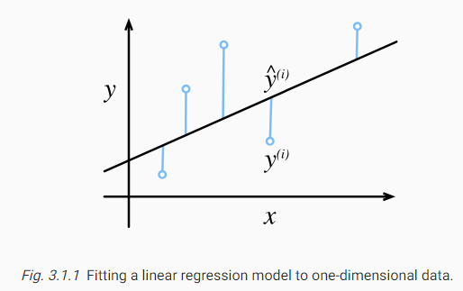
아래 Figure는 1차원 입력 문제에서 linear regression model의 적합성을 시각화 한 것입니다. (Fig. 3.1.1)
The constant1/2makes no real difference but proves to be notationally convenient, since it cancels out when we take the derivative of the loss. Because the training dataset is given to us, and thus is out of our control, the empirical error is only a function of the model parameters. InFig. 3.1.1, we visualize the fit of a linear regression model in a problem with one-dimensional inputs.
상수 1/2은 실제 차이는 없지만 손실의 미분을 취하면 상쇄되기 때문에 표기법상 편리한 것으로 입증되었습니다. 훈련 데이터 세트가 우리에게 제공되어 우리가 통제할 수 없기 때문에 경험적 오류는 모델 매개변수의 함수일 뿐입니다. 그림 3.1.1에서 우리는 1차원 입력 문제에 대한 선형 회귀 모델의 적합성을 시각화합니다.
derivative of the loss 란?
The derivative of the loss refers to the rate of change of the loss function with respect to the model's parameters. In machine learning and optimization, the loss function is a measure of how well the model performs on a given task or dataset. By taking the derivative of the loss function with respect to the model's parameters, we can determine the direction and magnitude of the steepest ascent or descent in the loss landscape.
손실 함수의 도함수는 모델의 파라미터에 대한 손실 함수의 변화율을 나타냅니다. 기계 학습과 최적화에서 손실 함수는 모델이 주어진 작업이나 데이터셋에서 얼마나 잘 수행되는지를 측정하는 척도입니다. 손실 함수의 도함수를 계산함으로써, 손실 랜드스케이프에서 가장 가파른 상승 또는 하강 방향과 크기를 결정할 수 있습니다.
Here are a few key points about the derivative of the loss:
손실의 도함수에 관한 몇 가지 주요한 사항은 다음과 같습니다:
Gradient: The derivative of the loss is often referred to as the gradient. It represents the vector of partial derivatives of the loss function with respect to each parameter of the model. 그래디언트: 손실의 도함수는 종종 그래디언트라고도 합니다. 이는 손실 함수의 각 파라미터에 대한 편미분의 벡터를 나타냅니다.
Optimization: The derivative of the loss is essential for optimization algorithms, such as gradient descent, which aim to minimize the loss function. By computing the gradient, we can update the model's parameters in the direction that reduces the loss. 최적화: 손실의 도함수는 그래디언트 디센트와 같은 최적화 알고리즘에서 필수적입니다. 손실 함수를 최소화하기 위해 그래디언트를 계산하여 손실을 줄이는 방향으로 모델의 파라미터를 업데이트할 수 있습니다.
Learning Rate: The derivative of the loss helps determine the step size or learning rate in optimization algorithms. It scales the magnitude of the parameter updates based on the steepness of the loss landscape. 학습률: 손실의 도함수는 최적화 알고리즘에서 스텝 크기 또는 학습률을 결정하는 데 도움을 줍니다. 손실 랜드스케이프의 가파른 정도에 따라 파라미터 업데이트의 크기를 조정합니다.
Backpropagation: In neural networks, the derivative of the loss is computed through the process of backpropagation. It involves propagating the gradients backward from the output layer to the input layer, using the chain rule of calculus, to efficiently compute the gradients with respect to the model's parameters. 역전파: 신경망에서 손실의 도함수는 역전파 과정을 통해 계산됩니다. 이는 미분 연쇄 법칙을 사용하여 그래디언트를 출력층에서 입력층으로 효율적으로 전파하여 모델의 파라미터에 대한 그래디언트를 계산하는 과정입니다.
Parameter Updates: The derivative of the loss guides the updates of the model's parameters during training. By descending along the negative gradient direction, the parameters are adjusted to improve the model's performance on the task. 파라미터 업데이트: 손실의 도함수는 학습 중에 모델의 파라미터 업데이트를 안내합니다. 음의 그래디언트 방향으로 하강함으로써 모델의 성능을 개선하기 위해 파라미터가 조정됩니다.
In summary, the derivative of the loss provides crucial information about the direction and magnitude of parameter updates that are necessary for optimizing and improving the model's performance during training.
***요약하면, 손실의 도함수는 학습 중에 모델의 파라미터 업데이트에 필요한 방향과 크기에 대한 중요한 정보를 제공합니다. 이를 통해 모델의 성능을 최적화하고 개선하는 데 필요한 파라미터 업데이트를 수행할 수 있습니다.***
Empirical Error 란?
Empirical error refers to the error or discrepancy between the predictions made by a model and the actual observed outcomes or labels in the training data. It is a measure of how well the model fits or approximates the training data.
경험적 오차(empirical error)는 모델의 예측과 훈련 데이터에서 관찰된 실제 결과 또는 레이블 사이의 오차나 불일치를 의미합니다. 이는 모델이 훈련 데이터에 얼마나 잘 맞는지 또는 근사하는지를 측정하는 척도입니다.
Here are a few key points about empirical error:
경험적 오차에 관한 몇 가지 주요한 사항은 다음과 같습니다:
Training Data: Empirical error is calculated based on the training data. The model's predictions on the training examples are compared to their actual labels or outcomes. 훈련 데이터: 경험적 오차는 훈련 데이터를 기반으로 계산됩니다. 모델의 예측값을 훈련 예제의 실제 레이블이나 결과와 비교합니다.
Measure of Fit: Empirical error quantifies the model's performance on the training data. It provides an indication of how well the model captures the patterns, relationships, or trends present in the training examples. 적합도 측정: 경험적 오차는 모델의 훈련 데이터에 대한 성능을 측정합니다. 이는 모델이 훈련 예제에 존재하는 패턴, 관계 또는 경향을 얼마나 잘 포착하는지를 나타냅니다.
Loss Function: Empirical error is typically evaluated using a loss function that measures the discrepancy between the predicted values and the actual labels. Common loss functions include mean squared error (MSE), cross-entropy loss, or absolute difference. 손실 함수: 경험적 오차는 일반적으로 예측값과 실제 레이블 사이의 불일치를 측정하는 손실 함수를 사용하여 평가됩니다. 일반적인 손실 함수로는 평균 제곱 오차(MSE), 크로스 엔트로피 손실, 절댓값 차이 등이 있습니다.
Minimization: During the training process, the model aims to minimize the empirical error by adjusting its parameters through optimization algorithms like gradient descent. The goal is to find the parameter values that yield the lowest empirical error on the training data. 최소화: 훈련 과정에서 모델은 경험적 오차를 최소화하기 위해 그래디언트 디센트와 같은 최적화 알고리즘을 통해 파라미터를 조정합니다. 목표는 훈련 데이터에서 경험적 오차를 최소화하는 파라미터 값을 찾는 것입니다.
Generalization: While empirical error measures the model's performance on the training data, it does not guarantee its performance on unseen or test data. The model may overfit the training data and perform poorly on new examples, indicating a lack of generalization. 일반화: 경험적 오차는 모델의 훈련 데이터에 대한 성능을 측정하지만, 새로운 데이터나 테스트 데이터에 대한 성능을 보장하지는 않습니다. 모델은 훈련 데이터에 과적합되어 새로운 예제에서 성능이 저하될 수 있으며, 이는 일반화 부족을 나타냅니다.
Validation and Test Error: To assess the model's generalization ability, it is important to evaluate its performance on separate validation or test datasets. These datasets provide a measure of the model's error on unseen data, which can be different from the empirical error. 검증 및 테스트 오차: 모델의 일반화 능력을 평가하기 위해 별도의 검증 또는 테스트 데이터셋에서 성능을 평가하는 것이 중요합니다. 이러한 데이터셋은 보이지 않은 데이터에 대한 모델의 오차를 제공하며, 이는 경험적 오차와 다를 수 있습니다.
In summary, empirical error represents the discrepancy between a model's predictions and the observed outcomes in the training data. It serves as a measure of how well the model fits the training examples, but additional evaluation on separate datasets is needed to assess its generalization performance.
요약하면, 경험적 오차는 모델의 예측과 훈련 데이터에서 관찰된 결과 사이의 오차를 나타냅니다. 이는 모델이 훈련 예제에 얼마나 잘 맞는지를 측정하는 지표이지만, 일반화 성능을 평가하기 위해서는 별도의 데이터셋에서 평가가 필요합니다.
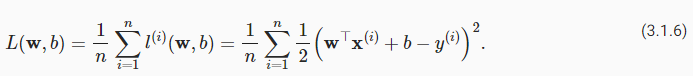
Note that large differences between estimatesy^**(i)and targetsy**(i)lead to even larger contributions to the loss, due to its quadratic form (this quadraticity can be a double-edge sword; while it encourages the model to avoid large errors it can also lead to excessive sensitivity to anomalous data). To measure the quality of a model on the entire dataset of nexamples, we simply average (or equivalently, sum) the losses on the training set:
추정치 y^**(i)와 목표 y**(i) 사이의 큰 차이는 2차 형식으로 인해 손실에 더 큰 기여를 한다는 점에 유의하세요(이 2차는 양날의 검이 될 수 있습니다. 큰 오류를 피하기 위해 모델을 사용하면 비정상적인 데이터에 대한 과도한 민감도가 발생할 수도 있습니다. n개의 예제로 구성된 전체 데이터세트에서 모델의 품질을 측정하려면 훈련 세트의 손실을 간단히 평균(또는 동등하게 합산)하면 됩니다.
estimates ŷ(i) 와 target y(i) 사이의 큰 차이는 loss의 quadratic form (2차 형태)로 인해 손실에 더 큰 기여를 이끈다는 겁니다.
이것은 양날의 검입니다. 모델이 large error들을 피할 수 있도록 하면 비정상적인 데이터에 대한 지나친 민감도를 유도할 수 있습니다.
n examples의 전체 dataset에 대한 모델의 quality를 측정하기 위해 우리는 간단하게 training set에 대한 losses의 평균 (or equivalently, sum) 을 구합니다.
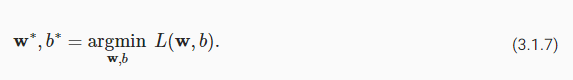
모델을 training 할 때 우리는 파라미터 (w*, b*)를 찾기를 원합니다.
그럼으로써 모든 traning examples에 걸쳐 총 loss를 minimize할 수 있기 때문입니다.
When training the model, we seek parameters (w∗,b∗) that minimize the total loss across all training examples:
모델을 훈련할 때 모든 훈련 예제에서 총 손실을 최소화하는 매개변수(w*,b*)를 찾습니다.
3.1.1.3. Analytic Solution
Unlike most of the models that we will cover, linear regression presents us with a surprisingly easy optimization problem. In particular, we can find the optimal parameters (as assessed on the training data) analytically by applying a simple formula as follows. First, we can subsume the biasbinto the parameterwby appending a column to the design matrix consisting of all 1s. Then our prediction problem is to minimize‖y−Xw‖2. As long as the design matrixXhas full rank (no feature is linearly dependent on the others), then there will be just one critical point on the loss surface and it corresponds to the minimum of the loss over the entire domain. Taking the derivative of the loss with respect towand setting it equal to zero yields:
우리가 다룰 대부분의 모델과 달리 선형 회귀는 놀라울 정도로 쉬운 최적화 문제를 제시합니다. 특히, 다음과 같은 간단한 공식을 적용하여 분석적으로 최적의 매개변수(훈련 데이터에서 평가된)를 찾을 수 있습니다. 먼저, 모두 1로 구성된 설계 행렬에 열을 추가하여 편향 b를 매개변수 w에 포함시킬 수 있습니다. 그러면 우리의 예측 문제는 "y−Xw"2를 최소화하는 것입니다. 설계 행렬 X가 전체 순위를 갖는 한(어떤 특성도 다른 특성에 선형적으로 종속되지 않음) 손실 표면에는 단 하나의 임계점이 있으며 이는 전체 도메인에 대한 손실의 최소값에 해당합니다. w에 대한 손실의 미분을 취하고 이를 0으로 설정하면 다음과 같습니다.
다음과 같은 간단한 공식을 적용하여 최적의 매개변수를 찾을 수 있습니다.
모든 것이 하나로 들어있는 design matrix에 하나의 column을 추가함으로서 bias b를 parameter w 에 포함시킬 수 있습니다.
이렇게 되면 우리의 prediction problem은 ||y - Xw||2 를 최소화 하는 것입니다..
design matrix X가 full rank (그 어떤 feature도 다른것에 linearly 종속되지 않는)를 갖는 한 loss surface에는 하나의 critical point만이 있게 됩니다. 그리고 이는 전체 domain에 대한 loss의 minimum에 해당합니다.
w에 대한 loss의 derivative (도함수)를 취하고 이를 0으로 설정하면 다음이 생성 됩니다.
Solving forwprovides us with the optimal solution for the optimization problem.
w를 풀면 최적화 문제에 대한 최적의 솔루션이 제공됩니다.
matrix (행렬) XTX가 invertible (가역적)일 때 이것은 unique할 것입니다.
예) design matrix의 columns들이 linearly independent (선형적으로 독립적)일 때 이것은 unique할 것입니다.
linear regression과 같은 간단한 문제는 analytic solution들을 admit할 수 있지만 이러한 운에 익숙해 지면 안됩니다.
Analytic solution이 훌륭한 mathematical analysis를 허용한다고 하더라도 analytic solution의 requirement는 너무 제한적입니다. 그래서 deep learning의 여러 흥미로운 측면들을 배제할 수 있는 위험성이 있습니다.
Note that this solution will only be unique when the matrixX⊤Xis invertible, i.e., when the columns of the design matrix are linearly independent(Golub and Van Loan, 1996).
이 솔루션은 행렬 X⊤X가 가역적일 때, 즉 설계 행렬의 열이 선형적으로 독립일 때에만 고유합니다(Golub and Van Loan, 1996).
While simple problems like linear regression may admit analytic solutions, you should not get used to such good fortune. Although analytic solutions allow for nice mathematical analysis, the requirement of an analytic solution is so restrictive that it would exclude almost all exciting aspects of deep learning.
선형 회귀와 같은 간단한 문제는 분석적 솔루션을 허용할 수 있지만 그러한 행운에 익숙해져서는 안 됩니다. 분석 솔루션을 사용하면 훌륭한 수학적 분석이 가능하지만 분석 솔루션의 요구 사항이 너무 제한적이어서 딥 러닝의 흥미로운 측면을 거의 모두 배제할 수 있습니다.
3.1.1.4 Minibatch Stochastic Gradient Descent
Fortunately, even in cases where we cannot solve the models analytically, we can still often train models effectively in practice. Moreover, for many tasks, those hard-to-optimize models turn out to be so much better that figuring out how to train them ends up being well worth the trouble.
다행스럽게도 모델을 분석적으로 해결할 수 없는 경우에도 실제로 모델을 효과적으로 훈련할 수 있는 경우가 많습니다. 더욱이, 많은 작업에서 최적화하기 어려운 모델은 훨씬 더 나은 것으로 판명되어 모델을 훈련하는 방법을 알아내는 것은 결국 문제를 해결할 가치가 충분히 있습니다.
The key technique for optimizing nearly every deep learning model, and which we will call upon throughout this book, consists of iteratively reducing the error by updating the parameters in the direction that incrementally lowers the loss function. This algorithm is calledgradient descent .
거의 모든 딥러닝 모델을 최적화하기 위한 핵심 기술이자 이 책 전체에서 사용할 핵심 기술은 손실 함수를 점진적으로 낮추는 방향으로 매개변수를 업데이트하여 오류를 반복적으로 줄이는 것으로 구성됩니다. 이 알고리즘을 경사하강법 gradient descent 이라고 합니다.
거의 모든 Deep learning model을 optimizing 하기 위한 key technique이자 이 책에서 계속 다룰 것은 loss function을 점진적으로 낮추는 방향으로 parameter들을 update함으로서 반복적으로 error들을 줄여 나가는 방법입니다.
이 알고리즘을 gradient descent라고 부릅니다.
Gradient descent 란?
Gradient descent is an optimization algorithm commonly used in machine learning and deep learning for minimizing the loss function and finding the optimal values of the model's parameters. It works by iteratively adjusting the parameter values in the direction of the negative gradient of the loss function.
경사 하강법(Gradient descent)은 머신러닝과 딥러닝에서 일반적으로 사용되는 최적화 알고리즘으로, 손실 함수를 최소화하고 모델의 파라미터의 최적값을 찾는 데 사용됩니다. 이는 손실 함수의 음의 그래디언트 방향으로 모델의 파라미터 값을 반복적으로 조정하는 방식으로 동작합니다.
Here are a few key points about gradient descent:
경사 하강법에 관한 주요한 사항은 다음과 같습니다:
Loss Function: Gradient descent requires a differentiable loss function that measures the discrepancy between the model's predictions and the true labels or outcomes. The goal is to minimize this loss function. 손실 함수: 경사 하강법은 모델의 예측과 실제 레이블 또는 결과 사이의 차이를 측정하는 미분 가능한 손실 함수가 필요합니다. 목표는 이 손실 함수를 최소화하는 것입니다.
Gradient: The gradient is a vector of partial derivatives of the loss function with respect to each parameter of the model. It indicates the direction and magnitude of the steepest ascent in the loss landscape. 그래디언트: 그래디언트는 손실 함수에 대한 각 파라미터의 편미분으로 이루어진 벡터입니다. 이는 손실 랜드스케이프에서 가파른 상승 방향과 크기를 나타냅니다.
Iterative Optimization: Gradient descent iteratively updates the model's parameters by taking small steps in the direction opposite to the gradient. It continues this process until it converges to a minimum of the loss function or reaches a predefined stopping criterion. 반복적 최적화: 경사 하강법은 반복적으로 파라미터 값을 업데이트합니다. 각 반복에서 그래디언트의 반대 방향으로 작은 단계를 취합니다. 이 과정은 손실 함수의 최소값에 수렴하거나 미리 정의된 중단 기준에 도달할 때까지 계속됩니다.
Learning Rate: The learning rate determines the step size or the magnitude of parameter updates in each iteration. It scales the gradient to control the speed of convergence and prevent overshooting or slow convergence. 학습률: 학습률은 각 반복에서 파라미터 업데이트의 크기 또는 스텝 크기를 결정합니다. 학습률은 그래디언트를 조절하여 수렴 속도를 제어하고 과도한 진동이나 느린 수렴을 방지합니다.
Batch and Stochastic Gradient Descent: Gradient descent can be performed on different subsets of the training data. Batch gradient descent updates the parameters using the gradients computed on the entire training dataset, while stochastic gradient descent updates the parameters using the gradients computed on individual training examples. 배치 경사 하강법과 확률적 경사 하강법: 경사 하강법은 훈련 데이터의 다른 부분집합에 대해 수행될 수 있습니다. 배치 경사 하강법은 전체 훈련 데이터셋에서 그래디언트를 계산하여 파라미터를 업데이트하고, 확률적 경사 하강법은 개별 훈련 예제에서 그래디언트를 계산하여 파라미터를 업데이트합니다.
Variants of Gradient Descent: Various variants of gradient descent have been developed to improve convergence speed and overcome limitations. Examples include mini-batch gradient descent, momentum-based methods, and adaptive learning rate methods like Adam. 경사 하강법의 변형: 수렴 속도를 개선하고 제약을 극복하기 위해 경사 하강법의 다양한 변형이 개발되었습니다. 예를 들어 미니배치 경사 하강법, 모멘텀 기반 방법, Adam과 같은 적응적 학습률 방법이 있습니다.
In summary, gradient descent is an iterative optimization algorithm that updates the model's parameters in the direction opposite to the gradient of the loss function. By minimizing the loss function, gradient descent helps to find the optimal parameter values for the model.
요약하면, 경사 하강법은 손실 함수의 그래디언트의 반대 방향으로 모델의 파라미터를 반복적으로 업데이트하는 최적화 알고리즘입니다. 손실 함수를 최소화함으로써 경사 하강법은 모델의 최적 파라미터 값을 찾는 데 도움을 줍니다.
The most naive application of gradient descent consists of taking the derivative of the loss function, which is an average of the losses computed on every single example in the dataset. In practice, this can be extremely slow: we must pass over the entire dataset before making a single update, even if the update steps might be very powerful(Liu and Nocedal, 1989). Even worse, if there is a lot of redundancy in the training data, the benefit of a full update is limited.
경사하강법의 가장 순진한 적용은 손실 함수의 미분을 취하는 것으로 구성됩니다. 손실 함수는 데이터 세트의 모든 단일 예에서 계산된 손실의 평균입니다. 실제로 이는 매우 느릴 수 있습니다. 업데이트 단계가 매우 강력하더라도 단일 업데이트를 수행하기 전에 전체 데이터 세트를 전달해야 합니다(Liu and Nocedal, 1989). 더 나쁜 것은 훈련 데이터에 중복성이 많으면 전체 업데이트의 이점이 제한된다는 것입니다.
Gradient Descent의 가장 간단한 방법은 dataset에 있는 모든 single example에서 계산된 손실의 평균인 손실 함수의 미분을 취하는 것입니다. 그 과정이 끝나면 파라미터를 업데이트 하게 됩니다.
이 방법은 간단하지만 느릴 수 있다는 단점이 있습니다.
우선 전체 데이터 세트가 전달 되어야 하고 그 다음에 단일 example별로 계산을 합니다. 이 dataset에 중복된 데이터가 많으면 전체 처리 시간이 더 길어 집니다.
The other extreme is to consider only a single example at a time and to take update steps based on one observation at a time. The resulting algorithm,stochastic gradient descent(SGD) can be an effective strategy(Bottou, 2010), even for large datasets. Unfortunately, SGD has drawbacks, both computational and statistical. One problem arises from the fact that processors are a lot faster multiplying and adding numbers than they are at moving data from main memory to processor cache. It is up to an order of magnitude more efficient to perform a matrix–vector multiplication than a corresponding number of vector–vector operations. This means that it can take a lot longer to process one sample at a time compared to a full batch. A second problem is that some of the layers, such as batch normalization (to be described inSection 8.5), only work well when we have access to more than one observation at a time.
또 다른 극단적인 방법은 한 번에 하나의 예만 고려하고 한 번에 하나의 관찰을 기반으로 업데이트 단계를 수행하는 것입니다. 결과 알고리즘인 확률적 경사 하강법(SGD)은 대규모 데이터 세트의 경우에도 효과적인 전략이 될 수 있습니다(Bottou, 2010). 불행하게도 SGD에는 계산적, 통계적 측면 모두에서 단점이 있습니다. 한 가지 문제는 프로세서가 주 메모리에서 프로세서 캐시로 데이터를 이동할 때보다 숫자를 곱하고 더하는 속도가 훨씬 빠르다는 사실에서 발생합니다. 해당 수의 벡터-벡터 연산보다 행렬-벡터 곱셈을 수행하는 것이 최대 10배 더 효율적입니다. 이는 전체 배치에 비해 한 번에 하나의 샘플을 처리하는 데 훨씬 더 오랜 시간이 걸릴 수 있음을 의미합니다. 두 번째 문제는 배치 정규화(8.5절에서 설명)와 같은 일부 레이어가 한 번에 둘 이상의 관측값에 접근할 수 있는 경우에만 잘 작동한다는 것입니다.
다른 극단적인 방법은 하나의 예만을 독립적으로 고려하여 계산해서 파라미터들을 업데이트 하는 것입니다.
이는 대규모 dataset의 경우에도 효과적으로 일을 처리할 수 있습니다.
이는 곱하고 더하는 연산보다 메인 메모리에서 프로세서 캐시로 데이터를 이동하는 것이 더 시간이 걸리기 때문에 시간이 더 오래 걸릴 수 있습니다. 또한 한번에 둘 이상의 관측값에 엑세스 할 수 있을 때만 잘 작동합니다.
The solution to both problems is to pick an intermediate strategy: rather than taking a full batch or only a single sample at a time, we take aminibatchof observations(Liet al., 2014). The specific choice of the size of the said minibatch depends on many factors, such as the amount of memory, the number of accelerators, the choice of layers, and the total dataset size. Despite all that, a number between 32 and 256, preferably a multiple of a large power of2, is a good start. This leads us tominibatch stochastic gradient descent.
두 문제에 대한 해결책은 중간 전략을 선택하는 것입니다. 즉, 전체 배치를 취하거나 한 번에 단일 샘플만 취하는 대신 관찰의 미니 배치를 취합니다(Li et al., 2014). 해당 미니배치 크기의 구체적인 선택은 메모리 양, 가속기 수, 레이어 선택, 전체 데이터세트 크기 등 여러 요소에 따라 달라집니다. 그럼에도 불구하고 32에서 256 사이의 숫자, 바람직하게는 2의 큰 거듭제곱의 배수가 좋은 시작입니다. 이는 미니배치 확률적 경사하강법으로 이어집니다.
두 방법의 단점을 극복하는 방법은 중간 전략을 선택하는 것입니다.
미니 배치들로 나눠서 가져오는 방법입니다.
이 방법을 minibatch stochastic gradient descent라고 부릅니다.
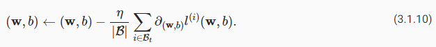
In its most basic form, in each iteration t, we first randomly sample a minibatchβtconsisting of a fixed number| β |of training examples. We then compute the derivative (gradient) of the average loss on the minibatch with respect to the model parameters. Finally, we multiply the gradient by a predetermined small positive valueη, called thelearning rate, and subtract the resulting term from the current parameter values. We can express the update as follows:
가장 기본적인 형태인 각 반복 t에서 먼저 고정된 수 | β | 훈련 예시. 그런 다음 모델 매개변수와 관련하여 미니배치의 평균 손실의 미분(기울기)을 계산합니다. 마지막으로, 기울기에 미리 결정된 작은 양수 값(학습률이라고 함)을 곱하고 현재 매개변수 값에서 결과 항을 뺍니다. 업데이트를 다음과 같이 표현할 수 있습니다.
가장 기본적인 형태는 각 iteration t에서 우선 training examples에 있는 고정된 숫자 |Β| 에서 랜덤하게 샘플 minibatch Βt를 가져옵니다. 그 다음 Model parameters와 관련하여 minibatch의 average loss의 derivative (gradient)를 계산합니다.
마지막으로 learning rate라고 하는 미리 정해진 small positive value n을 gradient에 곱합니다. 그리고 나서 현재 parameter value에서 result term을 뺍니다. 이는 다음과 같이 표현할 수 있습니다.
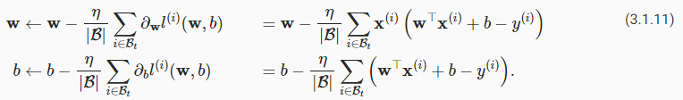
In summary, minibatch SGD proceeds as follows: (i) initialize the values of the model parameters, typically at random; (ii) iteratively sample random minibatches from the data, updating the parameters in the direction of the negative gradient. For quadratic losses and affine transformations, this has a closed-form expansion:
요약하면 미니배치 SGD는 다음과 같이 진행됩니다. (i) 일반적으로 무작위로 모델 매개변수의 값을 초기화합니다. (ii) 데이터에서 무작위 미니배치를 반복적으로 샘플링하여 음의 기울기 방향으로 매개변수를 업데이트합니다. 2차 손실 및 아핀 변환의 경우 이는 폐쇄 형식 확장을 갖습니다.
요약하면 minibatch SGD(Stochastic Gradient Descent)는 다음과 같이 진행됩니다.
1. Model parameters의 값을 random값으로 초기화 합니다.
2. data에서 random minibatches를 반복적으로 샘플링 한 후 negative gradient (음의 기울기) 방향으로 parameters를 업데이트 합니다.
SGD (Stochastic Gradient Descent) 란?
SGD stands for Stochastic Gradient Descent. It is an optimization algorithm commonly used in machine learning and deep learning for minimizing the loss function and finding the optimal parameters of a model.
SGD는 Stochastic Gradient Descent의 약자로, 머신러닝과 딥러닝에서 주로 사용되는 최적화 알고리즘입니다. 이 알고리즘은 손실 함수를 최소화하고 모델의 최적 매개변수를 찾기 위해 사용됩니다.
The term "stochastic" refers to the fact that the algorithm randomly selects a subset of training examples (also called a mini-batch) at each iteration, rather than using the entire training set. This sampling of mini-batches introduces randomness into the optimization process.
"Stochastic"이란 용어는 알고리즘이 각 반복에서 훈련 예제의 일부 (미니배치라고도 함)를 무작위로 선택하는 것을 의미합니다. 이러한 미니배치 샘플링은 최적화 과정에 무작위성을 도입합니다.
The term "gradient descent" refers to the process of iteratively updating the model parameters in the direction of the negative gradient of the loss function. The gradient represents the slope of the loss function with respect to each parameter, and moving in the direction of the negative gradient allows the algorithm to descend towards the minimum of the loss function.
"Gradient Descent"라는 용어는 손실 함수의 음의 그래디언트 방향으로 모델 매개변수를 반복적으로 업데이트하는 과정을 말합니다. 그래디언트는 각 매개변수에 대한 손실 함수의 기울기를 나타내며, 음의 그래디언트 방향으로 이동함으로써 알고리즘이 손실 함수의 최솟값에 접근할 수 있습니다.
In each iteration of SGD, the algorithm computes the gradients of the loss function with respect to the mini-batch of training examples and updates the model parameters accordingly. The size of the mini-batch can be adjusted, typically ranging from a few to a few hundred examples, and it affects the trade-off between computational efficiency and convergence speed.
SGD의 각 반복에서 알고리즘은 훈련 예제의 미니배치에 대한 손실 함수의 그래디언트를 계산하고 이를 사용하여 모델 매개변수를 업데이트합니다. 미니배치의 크기는 조정할 수 있으며, 일반적으로 몇 개에서 수백 개의 예제로 구성됩니다. 미니배치의 크기는 계산 효율성과 수렴 속도 사이의 균형을 조절하는 역할을 합니다.
SGD has become a popular optimization algorithm due to its simplicity and efficiency, particularly in large-scale machine learning tasks where the entire dataset cannot fit into memory. It allows models to be trained on subsets of data at a time, making it computationally feasible for large datasets.
SGD는 단순성과 효율성으로 인해 널리 사용되는 최적화 알고리즘으로, 전체 데이터 세트를 메모리에 저장할 수 없는 대규모 머신러닝 작업에서 특히 유용합니다. 이 알고리즘을 사용하면 모델을 한 번에 데이터의 일부로 훈련시킬 수 있으므로 대규모 데이터셋에 대한 계산적인 문제를 해결할 수 있습니다.
It's important to note that there are variations of SGD, such as mini-batch gradient descent and batch gradient descent, where the size of the mini-batch is set to 1 (pure SGD) or the entire training set, respectively. These variations have different characteristics in terms of computational efficiency and convergence properties.
중요한 점은 SGD의 변종이 있으며, 미니배치 그래디언트 디센트와 배치 그래디언트 디센트 등이 있습니다. 미니배치 크기가 각각 1(순수한 SGD) 또는 전체 훈련 세트인 경우입니다. 이러한 변종은 계산 효율성과 수렴 특성에 따라 다른 특징을 가지고 있습니다.
In summary, SGD is a widely used optimization algorithm that iteratively updates the model parameters using mini-batches of training examples and the gradients of the loss function. It enables efficient and scalable training of machine learning models.
요약하면, SGD는 훈련 예제의 미니배치와 손실 함수의 그래디언트를 사용하여 모델 매개변수를 반복적으로 업데이트하는 널리 사용되는 최적화 알고리즘입니다. 이를 통해 효율적이고 확장 가능한 머신러닝 모델을 훈련시킬 수 있습니다.
quandratic losses와 affine transformations에 대해서는 closed-form expansion이 있습니다.
Since we pick a minibatchβwe need to normalize by its size| β |. Frequently minibatch size and learning rate are user-defined. Such tunable parameters that are not updated in the training loop are calledhyperparameters. They can be tuned automatically by a number of techniques, such as Bayesian optimization(Frazier, 2018). In the end, the quality of the solution is typically assessed on a separatevalidation dataset(orvalidation set).
미니배치 β를 선택했으므로 크기 | β |. 미니배치 크기와 학습률은 사용자가 정의하는 경우가 많습니다. 훈련 루프에서 업데이트되지 않는 조정 가능한 매개변수를 하이퍼 매개변수라고 합니다. 베이지안 최적화(Frazier, 2018)와 같은 다양한 기술을 통해 자동으로 조정될 수 있습니다. 결국 솔루션의 품질은 일반적으로 별도의 검증 데이터 세트(또는 검증 세트)에서 평가됩니다.
minibatch Β를 선택했으므로 그것의 size |Β|에 대해 normalize 해야 합니다.
training loop에서 업데이트 되지 않은 조정 가능한 parameters를 hyperparameters라고 합니다.
결국 solution의 품질은 일반적으로 별도의 validation dataset (or validation set) 로 평가 됩니다.
After training for some predetermined number of iterations (or until some other stopping criterion is met), we record the estimated model parameters, denotedw^,b^. Note that even if our function is truly linear and noiseless, these parameters will not be the exact minimizers of the loss, nor even deterministic. Although the algorithm converges slowly towards the minimizers it typically will not find them exactly in a finite number of steps. Moreover, the minibatchesβused for updating the parameters are chosen at random. This breaks determinism.
미리 결정된 반복 횟수만큼(또는 다른 중지 기준이 충족될 때까지) 학습한 후 w^,b^로 표시된 추정 모델 매개변수를 기록합니다. 우리의 함수가 실제로 선형적이고 잡음이 없더라도 이러한 매개변수는 손실을 정확하게 최소화하지도 않고 결정적이지도 않습니다. 알고리즘은 최소화기를 향해 천천히 수렴하지만 일반적으로 유한한 수의 단계에서 정확하게 최소화기를 찾지는 않습니다. 더욱이, 매개변수 업데이트에 사용되는 미니배치 β는 무작위로 선택됩니다. 이것은 결정론을 깨뜨립니다.
미리 정해진 횟수 만큼 반복적으로 training 합니다. (또는 다른 기준이 충족될 때까지)
그 다음 ŵ,b̂로 표기된 estimated model parameters들로 기록합니다.
이러한 방법이 완벽할 수 는 없습니다. 또한 parameter를 update 하는데 사용되는 minibatch B 는 무작위로 선택됩니다.
This breaks determinism.
Linear regression happens to be a learning problem with a global minimum (wheneverXis full rank, or equivalently, wheneverX⊤Xis invertible). However, the loss surfaces for deep networks contain many saddle points and minima. Fortunately, we typically do not care about finding an exact set of parameters but merely any set of parameters that leads to accurate predictions (and thus low loss). In practice, deep learning practitioners seldom struggle to find parameters that minimize the losson training sets(Frankle and Carbin, 2018,Izmailovet al., 2018). The more formidable task is to find parameters that lead to accurate predictions on previously unseen data, a challenge calledgeneralization. We return to these topics throughout the book.
선형 회귀는 전역 최소값이 있는 학습 문제입니다(X가 전체 순위일 때마다 또는 X⊤X가 반전될 때마다). 그러나 심층 네트워크의 손실 표면에는 많은 안장점과 최소값이 포함되어 있습니다. 다행스럽게도 우리는 일반적으로 정확한 매개변수 세트를 찾는 데 관심이 없고 단지 정확한 예측(따라서 낮은 손실)으로 이어지는 매개변수 세트만 찾는 데 관심이 있습니다. 실제로 딥 러닝 실무자는 훈련 세트의 손실을 최소화하는 매개변수를 찾는 데 어려움을 겪는 경우가 거의 없습니다(Frankle and Carbin, 2018, Izmailov et al., 2018). 더 어려운 작업은 이전에 볼 수 없었던 데이터에 대한 정확한 예측으로 이어지는 매개변수를 찾는 것입니다. 이를 일반화라고 합니다. 우리는 책 전반에 걸쳐 이러한 주제로 돌아갑니다.
Linear regression은 global minimum이 있는 learning problem 입니다.
일반적으로 정확한 매개변수 세트가 아니라 정확한 예측을 이끌어 내는 매개변수 세트를 찾는데 더 관심이 있습니다.
실무에서 이러한 매개변수를 찾는데 큰 어려움은 없습니다.
어려울 때는 이전에 없었던 데이터에 대한 정확한 예측으로 이어지는 매개변수를 찾는 것인데 이를 generalization이라고 합니다.
3.1.1.5 Predictions
Given the modelw^⊤x+b^, we can now makepredictionsfor a new example, e.g., predicting the sales price of a previously unseen house given its areax1and agex2. Deep learning practitioners have taken to calling the prediction phaseinferencebut this is a bit of a misnomer—inferencerefers broadly to any conclusion reached on the basis of evidence, including both the values of the parameters and the likely label for an unseen instance. If anything, in the statistics literatureinferencemore often denotes parameter inference and this overloading of terminology creates unnecessary confusion when deep learning practitioners talk to statisticians. In the following we will stick topredictionwhenever possible.
모델 w^⊤x+b^가 주어지면 이제 새로운 예에 대한 예측을 할 수 있습니다. 예를 들어 면적 x1과 연령 x2를 고려하여 이전에 볼 수 없었던 주택의 판매 가격을 예측하는 것입니다. 딥 러닝 실무자들은 예측 단계 추론이라고 부르지만 이것은 약간 잘못된 명칭입니다. 추론은 매개변수의 값과 보이지 않는 인스턴스에 대한 가능한 레이블을 모두 포함하여 증거를 기반으로 도달한 모든 결론을 광범위하게 나타냅니다. 오히려 통계 문헌에서 추론은 매개변수 추론을 의미하는 경우가 더 많으며 이러한 용어의 과부하는 딥 러닝 실무자가 통계학자와 대화할 때 불필요한 혼란을 야기합니다. 다음에서는 가능할 때마다 예측을 고수하겠습니다.
ŵTx + b̂ 모델이 주어 졌을 때 이제 우리는 new example에 대한 predictions를 만들 수 있습니다.
예를 들어 면적 x1과 age x2가 주어진 이전에 못 보았던 집의 판매 가격을 예측하는 것입니다.
3.1.2. Vectorization for Speed
When training our models, we typically want to process whole minibatches of examples simultaneously. Doing this efficiently requires that we vectorize the calculations and leverage fast linear algebra libraries rather than writing costly for-loops in Python.
모델을 훈련할 때 일반적으로 예제의 전체 미니 배치를 동시에 처리하려고 합니다. 이를 효율적으로 수행하려면 Python에서 비용이 많이 드는 for 루프를 작성하는 대신 계산을 벡터화하고 빠른 선형 대수 라이브러리를 활용해야 합니다.
우리의 모델을 training 할 때 우리는 동시에 examples의 모든 minibatches를 처리하려고 합니다. 이것을 효과적으로 처리하려면 Python에서 고비용의 for 루프를 돌리는 대신 계산을 벡터화 하고 빠른 linear algebra 라이브러리를 활용해야 합니다.
To see why this matters so much, let’s consider two methods for adding vectors. To start, we instantiate two 10,000-dimensional vectors containing all 1s. In the first method, we loop over the vectors with a Python for-loop. In the second, we rely on a single call to+.
이것이 왜 그렇게 중요한지 알아보기 위해 벡터를 추가하는 두 가지 방법을 고려해 보겠습니다. 시작하려면 모두 1을 포함하는 두 개의 10,000차원 벡터를 인스턴스화합니다. 첫 번째 방법에서는 Python for-loop를 사용하여 벡터를 반복합니다. 두 번째에서는 +에 대한 단일 호출에 의존합니다.
이 방법이 왜 중요한지 설명하기 위해 벡터를 추가하는 두가지 방법을 보여드리겠습니다. 이것을 시작하려면 1만 차원의 벡터 두개를 초기화 할 겁니다.
초기화 하는 한 방법은 Python의 for 문을 사용해서 vectors에 루프를 돌립니다.
다른 방법은 +에 대한 단일 호출에 의존할 겁니다.
Pytorch
n = 10000
a = torch.ones(n)
b = torch.ones(n)
이 PyTorch 코드는 a와 b 두 개의 텐서를 1로 초기화합니다. 아래는 코드의 설명입니다:
n = 10000: 이 줄은 변수 n에 값 10000을 할당합니다. 이는 텐서(tensors ) a와 b의 크기 또는 길이를 나타냅니다.
a = torch.ones(n): 이 줄은 길이가 n (이 경우에는 10000)인 텐서 a를 생성하고 1로 채웁니다. torch.ones() 함수는 지정된 크기의 텐서를 생성하고 1로 채우는 데 사용됩니다.
b = torch.ones(n): 이 줄은 a와 동일한 길이인 (10000) 텐서 b를 생성하고 1로 채웁니다. 앞선 줄과 유사한 방식으로 동작합니다.
요약하면, 이 코드는 길이가 10000인 a와 b 두 개의 텐서를 생성하고 torch.ones() 함수를 사용하여 1로 초기화합니다.
Tensor란?
A tensor is a fundamental data structure in deep learning and scientific computing. It is a multi-dimensional array that can store and manipulate numerical data efficiently. Tensors are a generalization of vectors and matrices to higher dimensions and can represent scalars, vectors, matrices, and higher-dimensional arrays.
텐서(Tensor)는 딥러닝과 과학적 계산에 사용되는 기본적인 데이터 구조입니다. 텐서는 숫자 데이터를 효율적으로 저장하고 조작할 수 있는 다차원 배열입니다. 텐서는 벡터와 행렬을 고차원으로 일반화한 것으로, 스칼라, 벡터, 행렬 및 고차원 배열을 표현할 수 있습니다.
Here are a few key points about tensors:
텐서에 대한 주요한 사항은 다음과 같습니다:
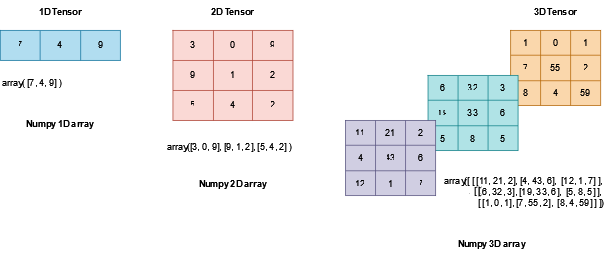
Dimensionality: Tensors can have any number of dimensions, also known as axes or ranks. Scalars have zero dimensions, vectors have one dimension, matrices have two dimensions, and tensors have more than two dimensions. 차원성: 텐서는 임의의 차원을 가질 수 있으며, 축 또는 순위라고도 합니다. 스칼라는 0차원, 벡터는 1차원, 행렬은 2차원이며, 텐서는 2차원 이상의 차원을 가집니다.
Shape: The shape of a tensor refers to the size of each dimension. For example, a 2D tensor with shape (3, 4) represents a matrix with 3 rows and 4 columns. The shape provides information about the tensor's structure and the arrangement of its elements. 형상: 텐서의 형상은 각 차원의 크기를 나타냅니다. 예를 들어, 형상이 (3, 4)인 2D 텐서는 3개의 행과 4개의 열로 구성된 행렬을 나타냅니다. 형상은 텐서의 구조와 요소의 배열 방식에 대한 정보를 제공합니다.
Data Types: Tensors can have different data types such as float, integer, or boolean. The choice of data type depends on the nature of the data being represented and the computations to be performed. 데이터 유형: 텐서는 부동 소수점, 정수, 부울 등 다양한 데이터 유형을 가질 수 있습니다. 데이터 유형의 선택은 표현하려는 데이터의 특성과 수행해야 할 계산에 따라 달라집니다.
Operations: Tensors support various mathematical operations and transformations such as addition, multiplication, dot product, matrix multiplication, reshaping, and slicing. These operations enable computations and transformations on large amounts of data efficiently. 연산: 텐서는 덧셈, 곱셈, 내적, 행렬 곱셈, 형태 변환, 슬라이싱, broadcasting, indexing 등 다양한 수학적 연산과 변환을 지원합니다. 이러한 연산을 통해 대량의 데이터에 대한 계산과 변환을 효율적으로 수행할 수 있습니다.
GPU Acceleration: Tensors can be efficiently processed on GPUs (Graphics Processing Units) for faster computations. Deep learning frameworks like PyTorch provide GPU acceleration, allowing tensor operations to leverage the parallel processing power of GPUs. GPU 가속화: 텐서는 GPU(그래픽 처리 장치)에서 효율적으로 처리될 수 있어 더 빠른 계산이 가능합니다. PyTorch와 TensorFlow와 같은 딥러닝 프레임워크는 GPU 가속화를 제공하여 텐서 연산이 GPU의 병렬 처리 능력을 활용할 수 있게 합니다.
Tensors are a foundational data structure in deep learning frameworks like PyTorch and TensorFlow. They enable efficient representation, manipulation, and computation of numerical data, making them essential for building and training deep learning models.
텐서는 PyTorch와 TensorFlow와 같은 딥러닝 프레임워크에서 핵심적인 데이터 구조입니다. 텐서는 숫자 데이터의 효율적인 표현, 조작 및 계산을 가능하게 하므로, 딥러닝 모델의 구축과 훈련에 필수적입니다.
Now we can benchmark the workloads. First, we add them, one coordinate at a time, using a for-loop.
이제 초기화 한 값을 for 루프로 돌려 보겠습니다.
c = torch.zeros(n)
t = time.time()
for i in range(n):
    c[i] = a[i] + b[i]
f'{time.time() - t:.5f} sec'
위 PyTorch 코드는 두 개의 텐서 a와 b의 요소별 덧셈을 수행하고 연산에 소요된 시간을 측정합니다. 코드를 설명하겠습니다:
c = torch.zeros(n): 이 줄은 a와 b와 동일한 길이인 c라는 텐서를 생성하고, torch.zeros() 함수를 사용하여 0으로 초기화합니다.
t = time.time(): 이 줄은 현재 시간을 기록합니다. time.time() 함수를 사용하여 현재 시점을 기준으로 시간을 측정합니다.
for i in range(n):: 이 줄은 0부터 n-1까지의 인덱스를 순회하는 반복문을 시작합니다.
c[i] = a[i] + b[i]: 반복문 내부에서 해당하는 인덱스의 a와 b의 요소를 요소별로 더한 결과를 c의 해당 인덱스에 할당합니다.
f'{time.time() - t:.5f} sec': 이 줄은 반복문이 실행되는 데 걸린 시간을 계산합니다. t에 기록된 시작 시간을 현재 시간에서 빼는 방식으로 시간을 측정합니다. 시간을 소수점 다섯 자리로 포맷하여 문자열로 표시하고, "sec"를 추가합니다.
요약하면, 이 코드는 a와 b와 같은 길이의 빈 텐서 c를 생성하고, a와 b의 요소별 덧셈을 반복문으로 수행하여 기록된 시간을 측정합니다. 경과된 시간은 소수점 다섯 자리로 포맷하여 "sec"과 함께 문자열로 표시됩니다.
위 코드를 실행한 결과 입니다.
for loop를 사용한 경우 0.13464초 걸렸습니다.
Alternatively, we rely on the reloaded+operator to compute the elementwise sum.
이제 각 element별로 합계를 계산하기 위해 +연산자를 사용하겠습니다.
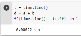
t = time.time()
d = a + b
f'{time.time() - t:.5f} sec'
실행 결과는 아래와 같습니다.
+연산자를 사용한 경우가 for loop를 사용한 경우보다 훨씬 처리 속도가 빠른 것을 볼 수 있습니다.
벡터화 하면 엄청난 속도 향상이 발생합니다. 또 직접 계산을 작성하지 않고 라이브러리를 이용하면 오류 가능성을 줄이고 code의 portability도 증가시킬 수 있습니다.
The second method is dramatically faster than the first. Vectorizing code often yields order-of-magnitude speedups. Moreover, we push more of the mathematics to the library so we do not have to write as many calculations ourselves, reducing the potential for errors and increasing portability of the code.
두 번째 방법은 첫 번째 방법보다 훨씬 빠릅니다. 코드를 벡터화하면 속도가 엄청나게 향상되는 경우가 많습니다. 더욱이 우리는 더 많은 수학을 라이브러리에 푸시하므로 스스로 많은 계산을 작성할 필요가 없으므로 오류 가능성이 줄어들고 코드 이식성이 향상됩니다.
3.1.3. The Normal Distribution and Squared Loss
So far we have given a fairly functional motivation of the squared loss objective: the optimal parameters return the conditional expectationE[Y∣X]whenever the underlying pattern is truly linear, and the loss assigns large penalties for outliers. We can also provide a more formal motivation for the squared loss objective by making probabilistic assumptions about the distribution of noise.
지금까지 우리는 제곱 손실 목표에 대해 상당히 기능적인 동기를 부여했습니다. 최적의 매개변수는 기본 패턴이 실제로 선형일 때마다 조건부 기대값 E[Y∣X]를 반환하고 손실은 이상치에 대해 큰 페널티를 할당합니다. 또한 잡음 분포에 대한 확률적 가정을 통해 제곱 손실 목표에 대한 보다 공식적인 동기를 제공할 수도 있습니다.
지금까지 squared loss (제곱된 손실) 을 왜 처리해야 되는지를 설명했습니다.
기본적인 패턴이 truly linear할 경우 optimal parameters는 조건부 기대값인 E[Y|X]를 반환합니다.
그리고 loss는 outliers에 대해 outsize penalties를 assign 합니다.
noise 분포에 대한 확률적 가정을 함으로서 squared loss objective에 대한 보다 formal 한 motivation을 제공할 수도 있습니다.
Linear regression was invented at the turn of the 19th century. While it has long been debated whether Gauss or Legendre first thought up the idea, it was Gauss who also discovered the normal distribution (also called theGaussian). It turns out that the normal distribution and linear regression with squared loss share a deeper connection than common parentage.
선형 회귀는 19세기 초에 발명되었습니다. 이 아이디어를 처음 생각해낸 사람이 가우스인지 르장드르인지 오랫동안 논쟁이 있었지만, 정규 분포(가우시안이라고도 함)를 발견한 사람도 가우스였습니다. 정규 분포와 손실 제곱을 사용한 선형 회귀는 공통 계열보다 더 깊은 연관성을 공유하는 것으로 나타났습니다.
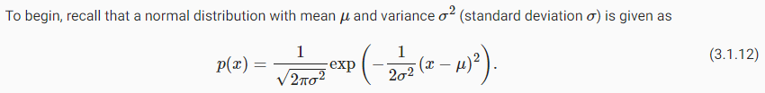
Linear regression (선형 회귀)와 normal distribution (정규 분포)를 시작하려면 다음을 기억하세요.
Below we define a function to compute the normal distribution.
위 코드는 정규 분포의 확률 밀도 함수를 계산하는 함수인 normal을 정의합니다. 코드를 설명하겠습니다:
def normal(x, mu, sigma):: 이 줄은 normal이라는 이름의 함수를 선언합니다. 이 함수는 x, mu, sigma라는 세 가지 입력 매개변수를 받습니다. 이 매개변수들은 각각 PDF를 평가할 값, 정규 분포의 평균, 그리고 표준 편차를 나타냅니다.
p = 1 / math.sqrt(2 * math.pi * sigma**2): 이 줄은 PDF를 정규화하는 계수 p를 계산합니다. 이 계수는 2π와 분포의 분산(sigma**2)의 곱의 제곱근의 역수로 계산됩니다.
return p * np.exp(-0.5 * (x - mu)**2 / sigma**2): 이 줄은 주어진 입력 값 x에서 PDF의 값을 계산하고 반환합니다. 이 식은 정규 분포 PDF의 공식을 사용하여 계산됩니다. x와 mu 사이의 제곱 차이를 2 * sigma**2로 나눈 후 음수로 지수화하고, 이를 계수 p와 곱합니다. np.exp() 함수를 사용하여 지수 값을 계산합니다.
요약하면, normal 함수는 주어진 입력 값 x에서 정규 분포의 확률 밀도 함수를 계산합니다. 이를 위해 제공된 평균 mu와 표준 편차 sigma를 사용합니다. 함수는 정규 분포 공식에 따라 해당 지점에서의 확률 밀도 값을 반환합니다.
PDF(Probability Density Function)란?
PDF stands for Probability Density Function. In the context of probability theory and statistics, a PDF is a mathematical function that describes the probability distribution of a continuous random variable. It specifies the relative likelihood of the random variable taking on a specific value or falling within a particular range of values.
PDF는 확률 밀도 함수(Probability Density Function)를 나타냅니다. 확률 이론과 통계학의 맥락에서, PDF는 연속적인 확률 변수의 확률 분포를 기술하는 수학적인 함수입니다. 이 함수는 특정 값을 가지거나 특정 값 범위 내에 떨어질 확률의 상대적인 가능성을 나타냅니다.
The PDF represents the probability density, which is the probability per unit of the variable. Unlike the probability of a specific outcome in a discrete distribution, the PDF gives the probability density over an interval in a continuous distribution. The integral of the PDF over a range of values gives the probability of the random variable falling within that range.
PDF는 단위별로 나타내는 확률 밀도로, 연속적인 분포에서 특정 구간 내에서의 확률을 나타냅니다. 이산적인 분포에서 특정 결과의 확률과 달리, PDF는 연속적인 분포에서 구간 내의 확률 밀도를 제공합니다. 구간 내에서의 확률은 PDF를 그 구간 상에서 적분함으로써 구할 수 있습니다.
In the given context, the normal function computes the PDF of a normal distribution. It calculates the probability density at a given input value x based on the mean mu and standard deviation sigma of the normal distribution. The PDF provides information about the relative likelihood of x occurring in the distribution.
주어진 맥락에서, normal 함수는 정규 분포의 확률 밀도 함수를 계산합니다. 이 함수는 주어진 입력 값 x에서 정규 분포의 평균 mu와 표준 편차 sigma를 기반으로 확률 밀도를 계산합니다. PDF는 x가 분포에서 발생할 상대적인 가능성에 대한 정보를 제공합니다.
We can now visualize the normal distributions.
이제 우리는 normal distributions (정규분포)를 시각화 할 수 있습니다.
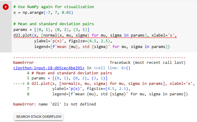
# Use NumPy again for visualization
x = np.arange(-7, 7, 0.01)

# Mean and standard deviation pairs
params = [(0, 1), (0, 2), (3, 1)]
d2l.plot(x, [normal(x, mu, sigma) for mu, sigma in params], xlabel='x',
         ylabel='p(x)', figsize=(4.5, 2.5),
         legend=[f'mean {mu}, std {sigma}' for mu, sigma in params])
위 코드는 NumPy와 이전에 정의한 normal 함수를 사용하여 세 가지 다른 정규 분포를 시각화하는 작업을 수행합니다. 코드를 설명하겠습니다:
x = np.arange(-7, 7, 0.01): 이 줄은 NumPy의 arange 함수를 사용하여 배열 x를 생성합니다. 이 함수는 -7부터 7까지 0.01 간격으로 값을 생성합니다. 이 값들은 정규 분포를 그릴 때 x축 값으로 사용됩니다.
params = [(0, 1), (0, 2), (3, 1)]: 이 줄은 params라는 이름의 튜플의 리스트를 정의합니다. 각 튜플은 정규 분포의 평균과 표준 편차 값을 나타냅니다. 이 경우 세 개의 페어가 지정되었습니다: (0, 1), (0, 2), (3, 1).
d2l.plot(x, [normal(x, mu, sigma) for mu, sigma in params], xlabel='x', ylabel='p(x)', figsize=(4.5, 2.5), legend=[f'mean {mu}, std {sigma}' for mu, sigma in params]): 이 줄은 d2l.plot() 함수를 사용하여 정규 분포를 시각화합니다. 다음 인수들을 사용합니다:
x: 플롯의 x축 값입니다.
[normal(x, mu, sigma) for mu, sigma in params]: 리스트 내장을 사용하여 각 분포에 대한 확률 밀도 값을 계산합니다. params 리스트를 반복하면서 각 평균과 표준 편차 조합에 대해 PDF를 계산합니다.
xlabel='x' 및 ylabel='p(x)': 플롯의 x축과 y축 레이블을 지정합니다.
figsize=(4.5, 2.5): 플롯의 크기를 설정합니다.
legend=[f'mean {mu}, std {sigma}' for mu, sigma in params]: 플롯의 범례 레이블을 설정합니다. 리스트 내장을 사용하여 각 평균과 표준 편차 조합에 대한 "mean mu, std sigma" 형식의 레이블을 생성합니다.
요약하면, 이 코드는 x축 값 배열 x를 생성하고, 세 개의 평균과 표준 편차 값 조합을 정의한 다음, normal 함수를 사용하여 해당하는 정규 분포를 그립니다. 결과 플롯은 각 분포의 확률 밀도 곡선을 보여주며, 범례는 각 곡선의 평균과 표준 편차 값을 나타냅니다.
나의 경우 위 코드를 실행하면 맨 처음에 d2l 모듈 인스톨에 실패했기 때문에 아래와 같은 에러가 나옵니다.
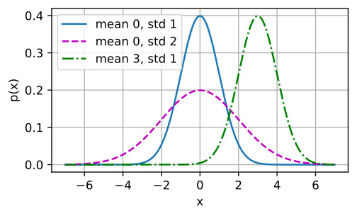
D2L 홈페이지를 보면 제대로 작동했을 경우 아래와 같은 표를 볼 수 있습니다.
mean (평균)을 바꾼다는 것은 x축을 따라 이동한다는 말입니다. 그리고 variance(분산)을 spreads하면 distribution(분포)가 넓어져서 peak가 낮아지게 됩니다.
Note that changing the mean corresponds to a shift along thex-axis, and increasing the variance spreads the distribution out, lowering its peak.
평균을 변경하는 것은 x축을 따라 이동하는 것에 해당하며, 분산을 늘리면 분포가 퍼져서 피크가 낮아집니다.
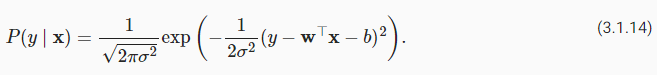
One way to motivate linear regression with squared loss is to assume that observations arise from noisy measurements, where the noiseεfollows the normal distributionN(0, σ 2):
제곱 손실을 사용하여 선형 회귀를 활성화하는 한 가지 방법은 관측값이 잡음이 있는 측정에서 발생한다고 가정하는 것입니다. 여기서 잡음 ε은 정규 분포 N(0, σ 2)를 따릅니다.
squared loss (손실 제곱)으로 linear regression (선형 회귀)를 유도하는 한 방법은 noise가 아래와 같이 인반적으로 분포되는 noisy measurements에서 관찰이 발생한다고 가정하는 것입니다.
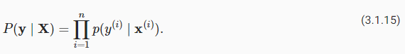
Thus, we can now write out thelikelihoodof seeing a particularyfor a givenxvia
이제 주어진 x에대한 특정 y를 볼 likelihood 아래와 같이 표기 할 수 있습니다.
As such, the likelihood factorizes. According tothe principle of maximum likelihood, the best values of parameterswandbare those that maximize thelikelihoodof the entire dataset:
likelihood는factorizes (인수분해) 됩니다. . the principle of maximum likehood에 따라 parameters w와 b의 최적의 값들은 전체 dataset의 likehood를 maximize 하는 겁니다.
likelihood 란?
Likelihood refers to the probability of observing a set of data given specific values of the parameters in a statistical model. It is a measure of how well the parameters of a model explain the observed data.
우도(likelihood)는 통계 모형의 특정 파라미터 값들에 대해 관측 데이터를 관찰할 확률을 의미합니다. 이는 모형의 파라미터가 관측된 데이터를 얼마나 잘 설명하는지를 측정하는 척도입니다.
In statistical inference, the likelihood function is constructed based on the assumption that the data are independent and identically distributed (i.i.d.). The likelihood function is defined as the probability of the observed data, viewed as a function of the model parameters. It represents the plausibility of the data given different values of the parameters.
통계적 추론에서 가능도 함수(likelihood function)는 데이터가 독립적이고 동일하게 분포되어 있다는 가정에 기반하여 구성됩니다. 가능도 함수는 모델 파라미터의 값으로 본 데이터의 확률로 정의됩니다. 이 함수는 다양한 파라미터 값에 대해 데이터가 얼마나 타당한지를 나타냅니다.
The likelihood is often used in maximum likelihood estimation (MLE), where the goal is to find the parameter values that maximize the likelihood function. This involves finding the parameter values that make the observed data most probable.
가능도는 최대 가능도 추정(maximum likelihood estimation, MLE)에서 자주 사용됩니다. 여기서 목표는 가능도 함수를 최대화하는 파라미터 값을 찾는 것입니다. 이는 관측된 데이터가 가장 확률적으로 발생할 수 있는 파라미터 값을 찾는 것을 의미합니다.
It is important to note that likelihood is different from probability. Probability quantifies the likelihood of a future event given known parameters, while likelihood quantifies the compatibility of observed data with different parameter values.
확률과 가능도는 서로 다른 개념임을 주목해야 합니다. 확률은 알려진 파라미터 값에 따라 미래 사건이 일어날 확률을 측정하는 반면, 가능도는 관측된 데이터와 다양한 파라미터 값들 사이의 호환성을 측정합니다.
In summary, likelihood represents the probability of observing a specific set of data given particular parameter values in a statistical model, and it plays a central role in statistical inference and parameter estimation.
요약하면, 가능도는 통계 모형의 특정 파라미터 값들에 대해 특정 데이터 집합을 관측할 확률을 나타내며, 통계적 추론과 파라미터 추정에 중요한 역할을 합니다.
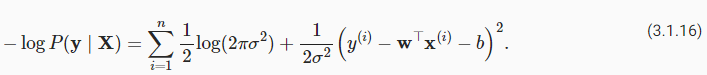
The equality follows since all pairs(x**(i),y**(i))were drawn independently of each other. Estimators chosen according to the principle of maximum likelihood are calledmaximum likelihood estimators. While, maximizing the product of many exponential functions, might look difficult, we can simplify things significantly, without changing the objective, by maximizing the logarithm of the likelihood instead. For historical reasons, optimizations are more often expressed as minimization rather than maximization. So, without changing anything, we canminimizethenegative log-likelihood, which we can express as follows:
모든 쌍 (x**(i),y**(i))이 서로 독립적으로 그려졌으므로 동등성이 따릅니다. 최대 우도 원칙에 따라 선택된 추정기를 최대 우도 추정기라고 합니다. 많은 지수 함수의 곱을 최대화하는 것이 어려워 보일 수 있지만 대신 우도의 로그를 최대화함으로써 목적을 변경하지 않고도 상황을 크게 단순화할 수 있습니다. 역사적 이유로 최적화는 최대화보다는 최소화로 표현되는 경우가 더 많습니다. 따라서 아무것도 변경하지 않고 음의 로그 가능성을 최소화할 수 있으며 다음과 같이 표현할 수 있습니다.
equiality는 모든 (x(i),y(i)) 쌍이 서로 독립적으로 그려진 것을 따릅니다.
maximum likelihood의 원칙에 의한 Estimators를 maximum likelihood estimators라고 합니다.
(exponential functions(지수함수)의 product를 maxmizing 하는 것은 어렵지만 이 likelihood의 알고리즘을 maxmization 함으로서 아무것도 바꾸지 않고 간단하게 처리할 수 있습니다.)
아무것도 변경하지 않고 우리는 negative log-likelihoo를 minimize 할 수 있습니다.
If we assume that σ is fixed, we can ignore the first term, because it does not depend onworb. The second term is identical to the squared error loss introduced earlier, except for the multiplicative constant 1/σ**2 . Fortunately, the solution does not depend on σ either. It follows that minimizing the mean squared error is equivalent to the maximum likelihood estimation of a linear model under the assumption of additive Gaussian noise.
σ가 고정되어 있다고 가정하면 첫 번째 항은 w 또는 b에 의존하지 않으므로 무시할 수 있습니다. 두 번째 항은 곱셈 상수 1/σ**2 를 제외하고 앞서 소개된 제곱 오차 손실과 동일합니다. 다행히도 해는 σ에도 의존하지 않습니다. 평균 제곱 오차를 최소화하는 것은 가산성 가우스 잡음을 가정한 선형 모델의 최대 우도 추정과 동일합니다.
σ 가 고정되어 있다고 가정하면 w 또는 b에 의존하지 않기 때문에 첫번째 항은 무시할 수 있습니다.
두번째 항은 multiplacative constant (곱셈상수) 1/σ2 만 빼면 이전에 봤던 squared error loss (제곱오차손실)와 동일합니다.
다행히 솔루션은 σ (sigma)에 의존하지 않습니다. mean squared error (평균 제곱 오차)를 minimizing 하는 것은 additive Gaussian noise (가산 가우시안 노이즈)의 가정 아래에서 linear model의 maximum likelihood estimation 하는 것과 동일합니다.
3.1.4. Linear Regression as a Neural Network
While linear models are not sufficiently rich to express the many complicated networks that we will introduce in this book, (artificial) neural networks are rich enough to subsume linear models as networks in which every feature is represented by an input neuron, all of which are connected directly to the output.
선형 모델은 이 책에서 소개할 많은 복잡한 네트워크를 표현할 만큼 풍부하지 않지만, (인공) 신경망은 선형 모델을 모든 기능이 입력 뉴런으로 표현되는 네트워크로 포함할 만큼 풍부합니다. 출력에 직접 연결됩니다.
linear model은 이 책에서 소개할 많은 복잡한 neural networks를 표현하기에 충분히 풍부하지는 않습니다.
neural network는 이 linear model들을 포함할 만큼 풍부합니다. (범위가 넓습니다.)
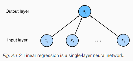
아래 그림은 linear regression을 neural network로 표현한 것입니다.
이 다이어 그램은 connectivity pattern들을 강조합니다. (각각의 input이 어떻게 output과 연결되는지...)
하지만 weights나 biases에 의해 취해진 특정 값들은 표시하지 못합니다.
Fig. 3.1.2depicts linear regression as a neural network. The diagram highlights the connectivity pattern, such as how each input is connected to the output, but not the specific values taken by the weights or biases.
그림 3.1.2는 선형 회귀를 신경망으로 묘사합니다. 다이어그램은 각 입력이 출력에 연결되는 방식과 같은 연결 패턴을 강조하지만 가중치나 편향이 취하는 특정 값은 강조하지 않습니다.
The inputs arex1,…,xd. We refer todas thenumber of inputsor thefeature dimensionalityin the input layer. The output of the network iso1. Because we are just trying to predict a single numerical value, we have only one output neuron. Note that the input values are allgiven. There is just a singlecomputedneuron. In summary, we can think of linear regression as a single-layer fully connected neural network. We will encounter networks with far more layers in later chapters.
입력은 x1,…,xd입니다. 우리는 d를 입력 수 또는 입력 레이어의 특징 차원이라고 부릅니다. 네트워크의 출력은 o1입니다. 우리는 단지 하나의 숫자 값을 예측하려고 하기 때문에 출력 뉴런이 하나만 있습니다. 입력 값은 모두 제공됩니다. 계산된 뉴런은 단 하나뿐입니다. 요약하면 선형 회귀는 단일 계층의 완전히 연결된 신경망으로 생각할 수 있습니다. 우리는 이후 장에서 훨씬 더 많은 레이어를 가진 네트워크를 접하게 될 것입니다.
입력은 x1,...xd 입니다. 여기서 d는 input의 수 혹은 input layer의 feature dimensionality를 나타냅니다.
이 network의 output은 o1입니다.
단일 숫자값을 예측하려고 하기 때문에 출력 뉴런은 하나만 있습니다. input 값들이 모두 제공되고 있음을 유의하세요.
여기에는 오직 하나의 computed neuron만이 있습니다.
요약하면 linear regression은 완전히 연결된 neural network의 single-layer라고 말할 수 있습니다.
다음 장에서는 훨씬 더 많은 계층을 가진 네트워크를 접하게 될 것입니다.
3.1.4.1. Biology
Because linear regression predates computational neuroscience, it might seem anachronistic to describe linear regression in terms of neural networks. Nonetheless, they were a natural place to start when the cyberneticists and neurophysiologists Warren McCulloch and Walter Pitts began to develop models of artificial neurons. Consider the cartoonish picture of a biological neuron inFig. 3.1.3, consisting ofdendrites(input terminals), thenucleus(CPU), theaxon(output wire), and theaxon terminals(output terminals), enabling connections to other neurons viasynapses.
선형 회귀는 계산 신경과학보다 앞서기 때문에 선형 회귀를 신경망 측면에서 설명하는 것은 시대착오적으로 보일 수 있습니다. 그럼에도 불구하고 사이버네틱스 학자이자 신경 생리학자인 Warren McCulloch와 Walter Pitts가 인공 뉴런 모델을 개발하기 시작했을 때 그것은 자연스러운 시작이었습니다. 수상돌기(입력 단자), 핵(CPU), 축삭(출력선), 그리고 축삭 말단(출력 단자)은 시냅스를 통해 다른 뉴런과의 연결을 가능하게 합니다.
linear regression은 computational neuroscience 보다 이전에 나왔습니다.
neural networks의 측면에서 linear regression을 묘사하는 것은 anachronistic (시대착오적)이라고 할 수도 있습니다.
그럼에도 불구하고 Warren McCulloch와 Walter Pitts가 artificial neurons 모델 개발을 시작했을 때 이는 자연스러운 출발점이었습니다.
아래 그림은 dendrites (수상돌기, input terminals), the nucleus(핵, CPU), the axon (축삭, output wire) 그리고 axon terninals (축삭 단자, 출력 단자)로 구성된 synapses를 통해 다른 뉴런에 연결할 수 있는 biological neuron을 그린 것입니다.
Fig. 3.1.3 The real neuron (source: “Anatomy and Physiology” by the US National Cancer Institute’s Surveillance, Epidemiology and End Results (SEER) Program).
Informationxi arriving from other neurons (or environmental sensors) is received in the dendrites. In particular, that information is weighted bysynaptic weightswi , determining the effect of the inputs, e.g., activation or inhibition via the productxiwi . The weighted inputs arriving from multiple sources are aggregated in the nucleus as a weighted sumy = ∑ixiwi+b, possibly subject to some nonlinear postprocessing via a functionσ(y). This information is then sent via the axon to the axon terminals, where it reaches its destination (e.g., an actuator such as a muscle) or it is fed into another neuron via its dendrites.
다른 뉴런(또는 환경 센서)에서 도착하는 정보 xi는 수상돌기에서 수신됩니다. 특히, 해당 정보는 시냅스 가중치 wi 에 의해 가중치가 부여되어 입력의 효과(예: 생성물 xiwi 를 통한 활성화 또는 억제)를 결정합니다. 여러 소스에서 도착하는 가중 입력은 가중 합 y = ∑ixiwi+b 로 핵에 집계되며, 함수 σ(y)를 통해 일부 비선형 후처리가 적용될 수 있습니다. 그런 다음 이 정보는 축삭을 통해 축삭 말단으로 전송되어 목적지(예: 근육과 같은 작동기)에 도달하거나 수상돌기를 통해 다른 뉴런에 공급됩니다.
다른 뉴런에서 도착한 xi은 dendrites (수상돌기)에서 수신됩니다. 특히 그 정보는 synaptic weights (시냅스 가중치) wi에 의해 가중되어 입력의 효과, 예를 들어 product xiwi를 통해 활성화 또는 억제를 결정합니다.여러 소스에서 도착하는 weighted inputs(가중 입력)은 weighted sum (가중합계) y = ∑ixiwi+b로 nucleus (핵)에서 집게 되며, 아마도 σ(y)를 통해 일부 nonlinear postprocessing (비선형 후처리)가 적용될 수 있습니다. 그런 다음 이 정보는 axon(축삭)을 통해 axon terminal (축삭 말단)으로 전송되어 목적지 (예: 근육과 같은 actuator -작동기-)에 도달하거나 dendrites(수상돌기)를 통해 다른 뉴런으로 공급됩니다.
Certainly, the high-level idea that many such units could be combined, provided they have the correct connectivity and learning algorithm, to produce far more interesting and complex behavior than any one neuron alone could express arises from our study of real biological neural systems. At the same time, most research in deep learning today draws inspiration from a much wider source. We invokeRussell and Norvig (2016)who pointed out that although airplanes might have beeninspiredby birds, ornithology has not been the primary driver of aeronautics innovation for some centuries. Likewise, inspiration in deep learning these days comes in equal or greater measure from mathematics, linguistics, psychology, statistics, computer science, and many other fields.
확실히, 그러한 많은 단위들이 올바른 연결성과 학습 알고리즘을 가지고 있다면 결합되어 하나의 뉴런만으로 표현할 수 있는 것보다 훨씬 더 흥미롭고 복잡한 행동을 생성할 수 있다는 높은 수준의 아이디어는 실제 생물학적 신경 시스템에 대한 우리의 연구에서 비롯되었습니다. 동시에 오늘날 딥러닝에 대한 대부분의 연구는 훨씬 더 광범위한 소스에서 영감을 얻습니다. 우리는 비행기가 새에서 영감을 받았을지라도 조류학이 몇 세기 동안 항공 혁신의 주요 동인이 되지 못했다고 지적한 Russell과 Norvig(2016)를 인용합니다. 마찬가지로 오늘날 딥 러닝에 대한 영감은 수학, 언어학, 심리학, 통계, 컴퓨터 과학 및 기타 여러 분야에서 동등하거나 더 큰 수준으로 나옵니다.
뇌의 구조는 아주 다양합니다. 어떤 것들은 다소 임의적으로 보이지만, 어떤 것들은 아주 규칙적인 구조를 가지고 있습니다. 예를 들면, 여러 곤충들의 시각 시스템은 아주 구조적입니다. 이 구조들에 대한 분석을 통해서 신경과학자들은 새로운 아키텍처를 제안하는데 영감을 받기도 하고, 어떤 경우에는 아주 성공적이었습니다. 하지만, 비행기가 새로부터 영감을 받아서 만들어 졌지만 차이가 많은 것과 같이, 이 둘의 직접적인 관계를 찾아보는 것은 오류가 되기도 합니다. 수학과 컴퓨터과학이 영감의 같은 근원이라고 볼 수 있습니다
이렇듯 deep learning은 신경망 연구의 도움을 많이 받습니다.
이 외에도 deep learning은 수학, 언어학, 심리학, 통게학, 컴퓨터 과학 밑 기타 여러 분야로 부터 많은 영감을 받습니다.
* Likelihood 란?
AI와 통계학의 맥락에서 "우도(likelihood)"는 특정 모델 또는 가설에서 특정 데이터 세트가 관측될 확률을 나타냅니다. 이는 모델이 관측된 데이터를 얼마나 잘 설명하는지를 측정하는 지표로, 통계적 추론에서 중요한 개념입니다.
간단히 설명하면 다음과 같습니다:
우도 함수(Likelihood Function): 통계 모델과 매개변수 세트가 주어졌을 때, 우도 함수는 해당 모델 및 특정 매개변수 값에서 관측된 데이터의 발생 확률을 측정합니다. 수학적으로는 종종 L(θ∣data)로 나타내며, 여기서 θ는 모델의 매개변수를 나타냅니다.
최대 우도 추정(MLE): 최대 우도 추정 원칙은 우도 함수를 최대화하는 모델 매개변수의 값을 찾는 것을 포함합니다. 이러한 매개변수 값은 관측된 데이터가 주어졌을 때 가장 가능성이 높다고 간주됩니다.
해석: 높은 우도는 주어진 모델과 매개변수 값에서 관측된 데이터가 발생할 가능성이 높음을 나타내며, 이는 좋은 적합성을 시사합니다. 반대로 낮은 우도는 모델이 관측된 데이터를 설명하는 데 적합하지 않을 수 있다는 것을 나타냅니다.
요약하면, AI와 통계에서의 우도는 특정 모델 및 매개변수화에서 관측된 데이터가 발생할 확률을 측정하는 지표로, 관측된 데이터를 기반으로 모델을 추정하고 선택하는 과정에서 중요한 개념입니다.
3.1.5. Summary
In this section, we introduced traditional linear regression, where the parameters of a linear function are chosen to minimize squared loss on the training set. We also motivated this choice of objective both via some practical considerations and through an interpretation of linear regression as maximimum likelihood estimation under an assumption of linearity and Gaussian noise. After discussing both computational considerations and connections to statistics, we showed how such linear models could be expressed as simple neural networks where the inputs are directly wired to the output(s). While we will soon move past linear models altogether, they are sufficient to introduce most of the components that all of our models require: parametric forms, differentiable objectives, optimization via minibatch stochastic gradient descent, and ultimately, evaluation on previously unseen data.
이 섹션에서는 훈련 세트의 제곱 손실을 최소화하기 위해 선형 함수의 매개변수를 선택하는 전통적인 선형 회귀를 소개했습니다. 우리는 또한 몇 가지 실제적인 고려 사항과 선형성 및 가우스 잡음을 가정한 최대 우도 추정으로 선형 회귀 해석을 통해 이러한 목표 선택에 동기를 부여했습니다. 계산상의 고려 사항과 통계와의 연결을 논의한 후 이러한 선형 모델이 입력이 출력에 직접 연결되는 간단한 신경망으로 어떻게 표현될 수 있는지 보여주었습니다. 곧 선형 모델을 완전히 넘어갈 것이지만, 모든 모델에 필요한 대부분의 구성요소(모수적 형태, 미분 가능한 목표, 미니배치 확률적 경사하강법을 통한 최적화, 궁극적으로 이전에 볼 수 없었던 데이터에 대한 평가)를 도입하는 데 충분합니다.
이번 섹션에서는 training set의 squared loss 를 최소화 하기 위해 linear function의 parameter를 선택하는 전통적인 linear regression을 소개했습니다. 이 외에도 몇가지 실용적인 고려사항과 선형성 및 가우시안 노이즈 가정 하에서 maximimum likelihood estimation 추정으로서 linear regression 해석을 통해 이러한 목표 선택에 설득력을 부여했습니다. 계산적인 고려사항과 통계와의 연관성을 논의한 후, 입력이 출력에 직접 연결되는 간단한 신경망 형태로 선형 모델을 표현하는 방법을 보여주었습니다. 선형 모델을 완전히 벗어나는 시점은 곧 찾아올 것이지만, 선형 모델은 우리 모델에 필요한 대부분의 구성 요소를 소개하는 데 충분합니다: 파라미터 형태, 미분 가능한 목적 함수, 미니배치 확률적 경사 하강법을 통한 최적화, 그리고 마지막으로 이전에 보지 못한 데이터에 대한 평가입니다.
머신러닝에서 중요한 요소는 학습 데이터, loss 함수, 최적화 알고리즘, 그리고 당연하지만 모델 자체입니다.
벡터화는 모든 것(수학)을 좋게 만들고, (코드를) 빠르게 만들어 줍니다.
objective 함수를 최소화하는 것과 maximum likelihood를 구하는 것은 같은 것입니다.
선형 모델도 뉴럴 모델입니다.
* 미분 가능 조건 ( differentiable conditions)
함수가 미분 가능하려면 특정 조건을 만족해야 합니다. 미분 가능성의 주요 조건은 다음과 같습니다:
연속성(Continuity): 함수는 미분이 고려되는 지점에서 연속적이어야 합니다. 연속성이 없거나 갑작스러운 모퉁이가 있는 경우 미분이 어려워질 수 있습니다.
도함수의 존재: 도함수를 정의하는 극한은 해당 지점에서 존재해야 합니다. 이는 함수의 그래프에 대한 접선의 기울기가 해당 지점에서 유한한 값을 가져야 함을 의미합니다.
부드러움(Smoothness): 함수는 급격한 변화나 모퉁이가 없어야 합니다. 갑작스러운 점프나 연속성이 없는 지점이 없는 부드러운 함수는 미분 가능성이 높습니다.
수직 접선이 없어야 함: 함수는 수직 접선을 가져서는 안 됩니다. 수직선은 기울기가 정의되지 않기 때문입니다.
커스프가 없어야 함: 함수는 접선의 방향이 갑작스럽게 바뀌는 지점이 없어야 합니다.
수직 아수피토트가 없어야 함: 함수는 해당 지점에서 수직 아수피토트를 가지면 안 됩니다. 이는 정의되지 않은 기울기를 유발할 수 있습니다.
신경망 및 최적화 관점에서 손실 함수는 중요한 구성 요소입니다. 미분 가능성이 거의 모든 곳에서 보장되면 확률적 경사 하강법과 같은 기울기 기반 최적화 방법을 효과적으로 사용할 수 있습니다. 이것은 모델 매개변수를 반복적으로 업데이트하기 위해 기울기 정보를 사용할 수 있게 합니다.
머신러닝에서 신경망을 교육하는 데 사용되는 많은 인기 있는 손실 함수들은 모델 매개변수에 대해 미분 가능하며, 이는 훈련 중에 손실 함수의 최소값을 찾기 위해 기울기 기반 최적화 알고리즘을 사용할 수 있게 합니다.