https://d2l.ai/chapter_linear-classification/softmax-regression-scratch.html

4.4. Softmax Regression Implementation from Scratch

Because softmax regression is so fundamental, we believe that you ought to know how to implement it yourself. Here, we limit ourselves to defining the softmax-specific aspects of the model and reuse the other components from our linear regression section, including the training loop.

softmax regression (회귀)는 매우 기본적이므로 직접 구현하는 방법을 알아야 한다고 생각합니다. 여기서는 모델의 softmax-specific 측면을 정의하는 것으로 제한하고 training loop-교육 루프-를 포함하여 linear regression-선형 회귀- 섹션의 다른 구성 요소를 재사용합니다.

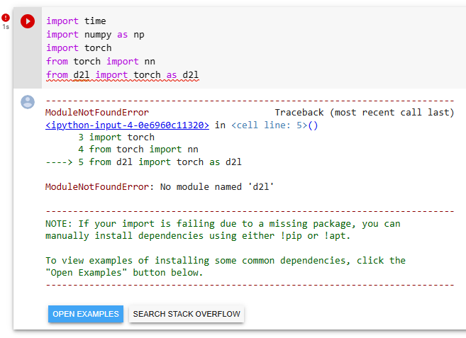
import torch
from d2l import torch as d2l

1. import torch: PyTorch 라이브러리를 임포트합니다. 이를 통해 PyTorch의 기능을 사용할 수 있습니다.
2. from d2l import torch as d2l: "d2l"이라는 이름의 패키지에서 "torch" 모듈을 임포트합니다. "d2l"은 Dive into Deep Learning (D2L) 도서의 교재와 관련된 유틸리티 함수와 모듈을 제공하는 패키지입니다. 이를 통해 D2L의 편리한 함수와 기능을 사용할 수 있습니다.

이 코드는 PyTorch를 사용하기 위해 torch 모듈을 임포트하고, D2L의 유틸리티 함수와 기능을 사용하기 위해 d2l 모듈을 임포트하는 역할을 합니다.

4.4.1. The Softmax

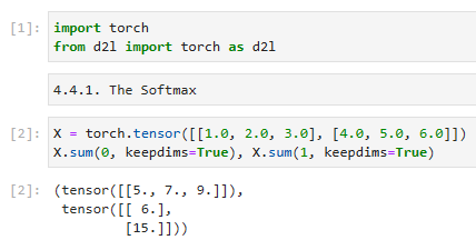
Let’s begin with the most important part: the mapping from scalars to probabilities. For a refresher, recall the operation of the sum operator along specific dimensions in a tensor, as discussed in Section 2.3.6 and Section 2.3.7. Given a matrix X we can sum over all elements (by default) or only over elements in the same axis. The axis variable lets us compute row and column sums:

가장 중요한 부분인 스칼라에서 확률로의 매핑부터 시작하겠습니다. 복습을 위해 섹션 2.3.6 및 섹션 2.3.7에서 설명한 대로 텐서의 특정 차원에 따른 합계 연산자의 작업을 상기하십시오. 행렬 X가 주어지면 모든 요소(기본값) 또는 동일한 축의 요소에 대해서만 합산할 수 있습니다. 축 변수를 사용하면 행과 열 합계를 계산할 수 있습니다.

X = torch.tensor([[1.0, 2.0, 3.0], [4.0, 5.0, 6.0]])
X.sum(0, keepdims=True), X.sum(1, keepdims=True)

1. X = torch.tensor([[1.0, 2.0, 3.0], [4.0, 5.0, 6.0]]): 입력 데이터인 X를 정의합니다. 이 예제에서는 크기가 2x3인 텐서입니다. 첫 번째 행은 [1.0, 2.0, 3.0]이고, 두 번째 행은 [4.0, 5.0, 6.0]입니다.
2. X.sum(0, keepdims=True): 열 방향으로 합계를 계산합니다. 0은 열 방향을 나타내는 축입니다. keepdims=True는 결과의 차원을 입력과 동일하게 유지하도록 지정합니다. 따라서 결과는 1x3 크기의 텐서가 됩니다. 열 방향으로 각 열의 원소를 합산한 결과입니다.
3. X.sum(1, keepdims=True): 행 방향으로 합계를 계산합니다. 1은 행 방향을 나타내는 축입니다. keepdims=True는 결과의 차원을 입력과 동일하게 유지하도록 지정합니다. 따라서 결과는 2x1 크기의 텐서가 됩니다. 행 방향으로 각 행의 원소를 합산한 결과입니다.

이 코드는 주어진 입력 텐서 X에서 열 방향과 행 방향으로 합계를 계산하는 예제입니다. 결과는 각각 1x3 크기와 2x1 크기의 텐서로 출력됩니다.

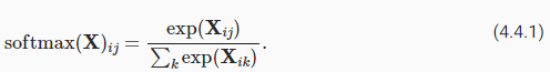
Computing the softmax requires three steps: (i) exponentiation of each term; (ii) a sum over each row to compute the normalization constant for each example; (iii) division of each row by its normalization constant, ensuring that the result sums to 1.

softmax를 계산하려면 세 단계가 필요합니다. (i) 각 항의 거듭제곱; (ii) 각 예에 대한 정규화 상수를 계산하기 위한 각 행에 대한 합계; (iii) 각 행을 정규화 상수로 나누어 결과 합계가 1이 되도록 합니다.

The (logarithm of the) denominator is called the (log) partition function. It was introduced in statistical physics to sum over all possible states in a thermodynamic ensemble. The implementation is straightforward:

분모(의 로그)를 (log) partition function(로그) 분할 함수라고 합니다. thermodynamic ensemble.열역학적 앙상블에서 가능한 모든 상태를 합산하기 위해 statistical physics 통계 물리학에 도입되었습니다. 구현은 간단합니다.

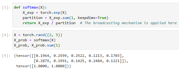
def softmax(X):
    X_exp = torch.exp(X)
    partition = X_exp.sum(1, keepdims=True)
    return X_exp / partition  # The broadcasting mechanism is applied here

1. def softmax(X):: softmax라는 함수를 정의합니다. 이 함수는 입력으로 주어진 텐서 X에 softmax 함수를 적용하여 반환합니다.
2. X_exp = torch.exp(X): 입력 텐서 X의 각 원소에 대해 지수 함수를 계산하여 X_exp에 저장합니다. 이는 softmax 함수의 분자 부분입니다.
3. partition = X_exp.sum(1, keepdims=True): X_exp의 행 방향으로 합계를 계산하여 partition에 저장합니다. keepdims=True는 결과의 차원을 입력과 동일하게 유지하도록 지정합니다. 이는 softmax 함수의 분모 부분입니다.
4. return X_exp / partition: 분자인 X_exp를 분모인 partition으로 나누어 softmax 함수의 결과를 반환합니다. 이 부분에서 브로드캐스팅 메커니즘이 적용됩니다. X_exp와 partition의 차원이 서로 다르더라도 알아서 확장되어 계산됩니다.

이 코드는 입력 텐서에 softmax 함수를 적용하는 함수를 정의한 것입니다. softmax 함수는 입력 텐서의 각 원소를 지수 함수로 변환한 후, 행 방향으로 합계를 계산하여 각 원소를 분모로 나누어 확률 분포를 생성합니다.

For any input X, we turn each element into a non-negative number. Each row sums up to 1, as is required for a probability. Caution: the code above is not robust against very large or very small arguments. While this is sufficient to illustrate what is happening, you should not use this code verbatim for any serious purpose. Deep learning frameworks have such protections built-in and we will be using the built-in softmax going forward.

모든 입력 X에 대해 각 요소를 음수가 아닌 숫자로 바꿉니다. 확률에 필요하므로 각 행의 합계는 1이 됩니다. 주의: 위의 코드는 매우 크거나 매우 작은 인수에 대해 강력하지 않습니다. 이는 무슨 일이 일어나고 있는지 설명하기에 충분하지만 심각한 목적을 위해 이 코드를 그대로 사용해서는 안 됩니다. 딥 러닝 프레임워크에는 이러한 보호 기능이 내장되어 있으며 앞으로도 내장된 softmax를 사용할 것입니다.

X = torch.rand((2, 5))
X_prob = softmax(X)
X_prob, X_prob.sum(1)

1. X = torch.rand((2, 5)): 2x5 크기의 랜덤한 값을 가진 텐서 X를 생성합니다.
2. X_prob = softmax(X): 앞서 설명한 softmax 함수를 X에 적용하여 확률 분포를 생성하여 X_prob에 저장합니다. X의 각 행은 확률로 변환됩니다.
3. X_prob: X_prob를 출력합니다. 이는 각 행이 확률로 변환된 텐서입니다.
4. X_prob.sum(1): X_prob의 행 방향으로 합계를 계산하여 출력합니다. 이를 통해 각 행의 원소들의 합이 1인지 확인할 수 있습니다.

이 코드는 주어진 입력 X에 softmax 함수를 적용하여 확률 분포를 생성하는 예시입니다. X는 랜덤한 값으로 초기화된 텐서이며, softmax 함수를 통해 각 행의 값을 확률로 변환합니다. X_prob은 확률로 변환된 텐서이며, X_prob.sum(1)을 통해 각 행의 원소들의 합이 1인지 확인할 수 있습니다.

4.4.2. The Model

We now have everything that we need to implement the softmax regression model. As in our linear regression example, each instance will be represented by a fixed-length vector. Since the raw data here consists of 28×28 pixel images, we flatten each image, treating them as vectors of length 784. In later chapters, we will introduce convolutional neural networks, which exploit the spatial structure in a more satisfying way.

이제 softmax 회귀(regression ) 모델을 구현하는 데 필요한 모든 것이 있습니다. linear regression 선형 회귀 예제에서와 같이 각 인스턴스는 fixed-length vector-고정 길이 벡터-로 표시됩니다. 여기서 원시 데이터는 28X28 픽셀 이미지로 구성되어 있으므로 각 이미지를 평면화하여 길이가 784인 벡터로 취급합니다. 이후 장에서는 공간 구조를 보다 만족스럽게 활용하는 convolutional neural networks-컨벌루션 신경망-을 소개합니다.

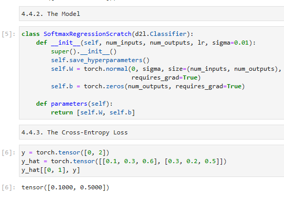
In softmax regression, the number of outputs from our network should be equal to the number of classes. Since our dataset has 10 classes, our network has an output dimension of 10. Consequently, our weights constitute a 784×10 matrix plus a 1×10 dimensional row vector for the biases. As with linear regression, we initialize the weights W with Gaussian noise. The biases are initialized as zeros.

softmax 회귀에서 네트워크의 출력 수는 클래스 수와 같아야 합니다. 데이터 세트에 10개의 클래스가 있으므로 네트워크의 출력 차원은 10입니다. 결과적으로 가중치는 편향에 대한 1X10 차원 행 벡터와 784 X 10 행렬을 구성합니다. linear regression-선형 회귀-와 마찬가지로 가중치 W를 Gaussian noise-가우시안 노이즈-로 초기화합니다. biases -편향-은 0으로 초기화됩니다.

class SoftmaxRegressionScratch(d2l.Classifier):
    def __init__(self, num_inputs, num_outputs, lr, sigma=0.01):
        super().__init__()
        self.save_hyperparameters()
        self.W = torch.normal(0, sigma, size=(num_inputs, num_outputs),
                              requires_grad=True)
        self.b = torch.zeros(num_outputs, requires_grad=True)

    def parameters(self):
        return [self.W, self.b]

1. class SoftmaxRegressionScratch(d2l.Classifier): SoftmaxRegressionScratch 클래스를 정의합니다. 이 클래스는 d2l.Classifier 클래스를 상속받습니다.
2. def __init__(self, num_inputs, num_outputs, lr, sigma=0.01): 클래스의 초기화 메서드입니다. 입력으로 num_inputs (입력 특성의 수), num_outputs (클래스의 수), lr (학습률), sigma (가중치 초기화를 위한 표준 편차)를 받습니다.
3. super().__init__(): 상위 클래스인 d2l.Classifier의 초기화 메서드를 호출합니다.
4. self.save_hyperparameters(): 하이퍼파라미터를 저장합니다.
5. self.W = torch.normal(0, sigma, size=(num_inputs, num_outputs), requires_grad=True): 크기가 (num_inputs, num_outputs)인 가중치 행렬 self.W를 생성합니다. 가중치는 평균이 0이고 표준 편차가 sigma인 정규 분포로부터 무작위로 초기화되며, requires_grad=True를 설정하여 역전파를 통해 학습될 수 있도록 설정합니다.
6. self.b = torch.zeros(num_outputs, requires_grad=True): 길이가 num_outputs인 편향 벡터 self.b를 생성합니다. 모든 요소가 0인 초기값으로 설정되며, requires_grad=True를 설정하여 역전파를 통해 학습될 수 있도록 설정합니다.
7. def parameters(self): 모델의 학습 가능한 파라미터를 반환하는 메서드입니다. self.W와 self.b를 리스트로 묶어 반환합니다.

이 코드는 Softmax 회귀 모델을 Scratch에서 구현한 클래스입니다. SoftmaxRegressionScratch 클래스는 d2l.Classifier를 상속받으며, 가중치와 편향을 초기화하고 학습 가능한 파라미터를 반환하는 기능을 포함하고 있습니다. 이 클래스를 사용하여 Softmax 회귀 모델을 구현하고 학습시킬 수 있습니다.

The code below defines how the network maps each input to an output. Note that we flatten each 28×28 pixel image in the batch into a vector using reshape before passing the data through our model.

아래 코드는 네트워크가 각 입력을 출력에 매핑하는 방법을 정의합니다. 모델을 통해 데이터를 전달하기 전에 reshape를 사용하여 배치의 각 28 X 28 픽셀 이미지를 벡터로 병합합니다.

@d2l.add_to_class(SoftmaxRegressionScratch)
def forward(self, X):
    X = X.reshape((-1, self.W.shape[0]))
    return softmax(torch.matmul(X, self.W) + self.b)

이 코드는 SoftmaxRegressionScratch 클래스에 forward 메서드를 추가하는 부분입니다. 코드를 한 줄씩 설명해드리겠습니다.

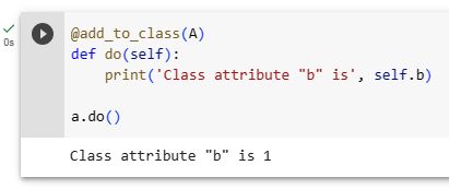
1. @d2l.add_to_class(SoftmaxRegressionScratch): d2l.add_to_class 데코레이터를 사용하여 SoftmaxRegressionScratch 클래스에 메서드를 추가합니다.
2. def forward(self, X): forward 메서드를 정의합니다. 이 메서드는 입력 데이터 X를 받습니다.
3. X = X.reshape((-1, self.W.shape[0])): 입력 데이터 X를 크기가 (배치 크기, 입력 특성의 수)인 형태로 변형합니다. 이를 통해 배치 처리가 가능하도록 준비합니다.
4. return softmax(torch.matmul(X, self.W) + self.b): 입력 데이터 X와 가중치 행렬 self.W 그리고 편향 벡터 self.b를 사용하여 Softmax 함수를 적용한 결과를 반환합니다. 입력 데이터와 가중치 행렬을 행렬 곱셈한 후 편향 벡터를 더한 다음, 이를 Softmax 함수에 적용하여 예측값을 계산합니다.

이렇게 forward 메서드를 추가하여 입력 데이터에 대한 예측값을 계산할 수 있게 되었습니다. 이 메서드를 사용하여 Softmax 회귀 모델을 구현한 SoftmaxRegressionScratch 클래스의 객체에 입력 데이터를 전달하면 해당 입력에 대한 예측값을 얻을 수 있습니다.

4.4.3. The Cross-Entropy Loss

Next we need to implement the cross-entropy loss function (introduced in Section 4.1.2). This may be the most common loss function in all of deep learning. At the moment, applications of deep learning easily cast classification problems far outnumber those better treated as regression problems.

다음으로 cross-entropy loss function-교차 엔트로피 손실 함수-를 구현해야 합니다(섹션 4.1.2에서 소개됨). 이것은 모든 딥 러닝에서 가장 일반적인 loss function-손실 함수-일 수 있습니다. 현재 딥 러닝의 응용 프로그램은 classification problems-분류 문제-를 쉽게 캐스팅하여 regression problems-회귀 문제-로 더 잘 처리되는 문제보다 훨씬 많습니다.

Recall that cross-entropy takes the negative log-likelihood of the predicted probability assigned to the true label. For efficiency we avoid Python for-loops and use indexing instead. In particular, the one-hot encoding in y allows us to select the matching terms in y^.

cross-entropy-교차 엔트로피-는 실제 레이블에 할당된 예측 확률의 negative log-likelihood-음의 로그 가능성-을 취한다는 점을 상기하십시오. 효율성을 위해 Python for-loops를 피하고 대신 인덱싱을 사용합니다. 특히 y의 one-hot encoding-원-핫 인코딩-을 사용하면 y^에서 일치하는 용어를 선택할 수 있습니다.

To see this in action we create sample data y_hat with 2 examples of predicted probabilities over 3 classes and their corresponding labels y. The correct labels are 0 and 2 respectively (i.e., the first and third class). Using y as the indices of the probabilities in y_hat, we can pick out terms efficiently.

이를 실제로 확인하기 위해 3개 클래스에 대한 predicted probabilities-예측 확률-의 2개 예와 해당 레이블 y로 샘플 데이터 y_hat을 만듭니다. 올바른 레이블은 각각 0과 2입니다(즉, 첫 번째 및 세 번째 클래스). y를 y_hat의 확률 지수로 사용하면 terms -용어-를 효율적으로 선택할 수 있습니다.

y = torch.tensor([0, 2])
y_hat = torch.tensor([[0.1, 0.3, 0.6], [0.3, 0.2, 0.5]])
y_hat[[0, 1], y]

이 코드는 y_hat 텐서에서 인덱스를 사용하여 특정 위치의 값을 선택하는 부분입니다. 코드를 한 줄씩 설명해드리겠습니다.

1. y = torch.tensor([0, 2]): 정수로 이루어진 텐서 y를 생성합니다. y는 선택할 인덱스 값으로 사용됩니다.
2. y_hat = torch.tensor([[0.1, 0.3, 0.6], [0.3, 0.2, 0.5]]): y_hat 텐서를 생성합니다. y_hat은 예측값으로 이루어진 2차원 텐서입니다.
3. y_hat[[0, 1], y]: y_hat 텐서에서 [0, 1] 위치의 행과 y 텐서의 값에 해당하는 열의 값들을 선택합니다. 즉, 첫 번째 행의 y[0] 값에 해당하는 열의 값과 두 번째 행의 y[1] 값에 해당하는 열의 값을 선택합니다.

결과적으로, y_hat[[0, 1], y]는 y_hat 텐서에서 첫 번째 행의 0번 열의 값과 두 번째 행의 2번 열의 값을 선택하여 반환합니다.

Now we can implement the cross-entropy loss function by averaging over the logarithms of the selected probabilities.

이제 선택한 probabilities-확률-의 logarithms -로그-를 평균화하여  cross-entropy loss function-교차 엔트로피 손실 함수-를 구현할 수 있습니다.

def cross_entropy(y_hat, y):
    return -torch.log(y_hat[list(range(len(y_hat))), y]).mean()

cross_entropy(y_hat, y)

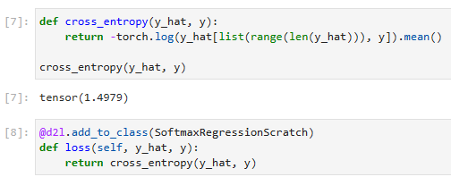
이 코드는 크로스 엔트로피 손실 함수를 계산하는 부분입니다. 코드를 한 줄씩 설명해드리겠습니다.

1. def cross_entropy(y_hat, y): cross_entropy라는 함수를 정의합니다. 이 함수는 y_hat과 y를 입력으로 받습니다. y_hat은 예측값, y는 실제 레이블로 구성된 텐서입니다.
2. -torch.log(y_hat[list(range(len(y_hat))), y]): y_hat 텐서의 예측값들 중에서 실제 레이블 y에 해당하는 위치의 로그값을 계산합니다. list(range(len(y_hat)))는 0부터 y_hat의 길이까지의 숫자 리스트를 생성하며, 이는 행 인덱스를 나타냅니다. y는 열 인덱스로 사용됩니다. 따라서 y_hat[list(range(len(y_hat))), y]는 y_hat에서 실제 레이블에 해당하는 위치의 값을 선택합니다.
3. .mean(): 선택된 값들의 평균을 계산합니다.

결과적으로, cross_entropy(y_hat, y)는 예측값 y_hat과 실제 레이블 y를 이용하여 크로스 엔트로피 손실을 계산한 결과를 반환합니다.

@d2l.add_to_class(SoftmaxRegressionScratch)
def loss(self, y_hat, y):
    return cross_entropy(y_hat, y)

위의 코드는 SoftmaxRegressionScratch 클래스에 loss 메서드를 추가하는 부분입니다. 코드를 한 줄씩 설명해드리겠습니다.

1. @d2l.add_to_class(SoftmaxRegressionScratch): d2l 모듈의 add_to_class 데코레이터를 사용하여 SoftmaxRegressionScratch 클래스에 메서드를 추가합니다.
2. def loss(self, y_hat, y): loss라는 메서드를 정의합니다. 이 메서드는 y_hat과 y를 입력으로 받습니다. y_hat은 예측값, y는 실제 레이블로 구성된 텐서입니다.
3. return cross_entropy(y_hat, y): cross_entropy 함수를 호출하여 y_hat과 y를 이용하여 크로스 엔트로피 손실을 계산한 결과를 반환합니다.

결과적으로, loss 메서드는 SoftmaxRegressionScratch 클래스의 예측값 y_hat과 실제 레이블 y를 이용하여 크로스 엔트로피 손실을 계산한 결과를 반환합니다. 이렇게 추가된 loss 메서드는 모델의 학습 및 평가 과정에서 사용될 수 있습니다.

4.4.4. Training

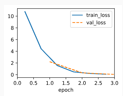
We reuse the fit method defined in Section 3.4 to train the model with 10 epochs. Note that both the number of epochs (max_epochs), the minibatch size (batch_size), and learning rate (lr) are adjustable hyperparameters. That means that while these values are not learned during our primary training loop, they still influence the performance of our model, bot vis-a-vis training and generalization performance. In practice you will want to choose these values based on the validation split of the data and then to ultimately evaluate your final model on the test split. As discussed in Section 3.6.3, we will treat the test data of Fashion-MNIST as the validation set, thus reporting validation loss and validation accuracy on this split.

섹션 3.4에서 정의한 fit method-적합 방법-을 재사용하여 10 epoch로 모델을 훈련합니다. Epoch 수(max_epochs), minibatch 크기(batch_size) 및 학습률(lr)은 모두 조정 가능한 hyperparameters-하이퍼파라미터-입니다. 즉, 이러한 값은 기본 교육 루프 중에 학습되지 않지만 여전히 모델의 성능, bot vis-a-vis training-봇 대비 교육- 및 generalization performance-일반화 성능-에 영향을 미칩니다. 실제로는 데이터의 validation split-검증 분할-을 기반으로 이러한 값을 선택한 다음 궁극적으로 test split-테스트 분할-에서 최종 모델을 평가하기를 원할 것입니다. 섹션 3.6.3에서 설명한 것처럼 Fashion-MNIST의 테스트 데이터를 validation set-유효성 검사 세트-로 취급하여 이 분할에서 validation loss -유효성 검사 손실- 및 validation accuracy on this split-유효성 검사 정확도-를 보고합니다.

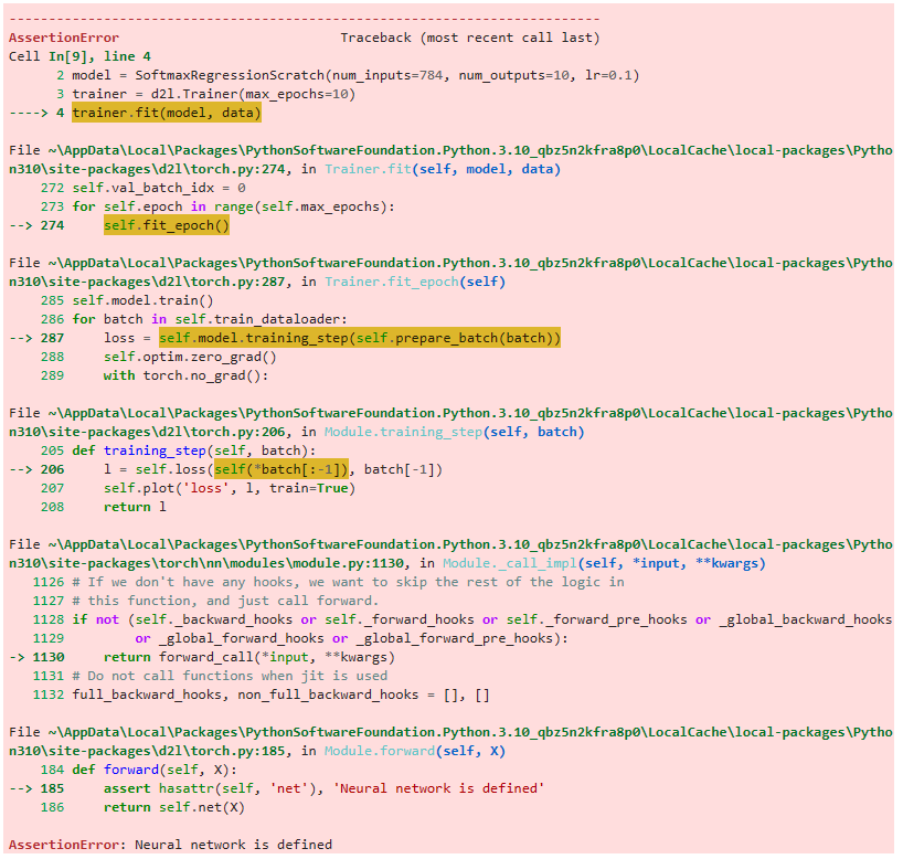
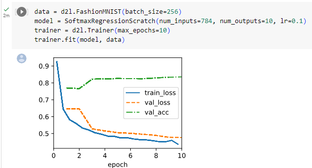
data = d2l.FashionMNIST(batch_size=256)
model = SoftmaxRegressionScratch(num_inputs=784, num_outputs=10, lr=0.1)
trainer = d2l.Trainer(max_epochs=10)
trainer.fit(model, data)

위의 코드는 FashionMNIST 데이터셋을 사용하여 Softmax 회귀 모델을 학습하는 과정을 보여줍니다. 코드를 한 줄씩 설명해드리겠습니다.

1. data = d2l.FashionMNIST(batch_size=256): d2l 모듈의 FashionMNIST 클래스를 사용하여 FashionMNIST 데이터셋을 생성합니다. 배치 크기는 256로 설정되었습니다.
2. model = SoftmaxRegressionScratch(num_inputs=784, num_outputs=10, lr=0.1): SoftmaxRegressionScratch 클래스의 인스턴스인 model을 생성합니다. 입력 특성 수는 784이고 출력 클래스 수는 10입니다. 학습률은 0.1로 설정되었습니다.
3. trainer = d2l.Trainer(max_epochs=10): d2l 모듈의 Trainer 클래스를 사용하여 훈련을 관리하는 trainer 객체를 생성합니다. 최대 에포크 수는 10으로 설정되었습니다.
4. trainer.fit(model, data): trainer 객체의 fit 메서드를 호출하여 모델 model과 데이터셋 data를 이용하여 모델을 학습시킵니다.

결과적으로, 위의 코드는 FashionMNIST 데이터셋을 사용하여 Softmax 회귀 모델을 10 에포크 동안 학습하는 과정을 보여줍니다. Trainer 클래스를 사용하여 모델의 학습을 관리하며, 학습된 모델은 model 객체에 저장됩니다.

Local에서 돌린 결과

CoLab에서 돌린 결과

4.4.5. Prediction

Now that training is complete, our model is ready to classify some images.

이제 교육이 완료되었으므로 모델은 일부 이미지를 분류할 준비가 되었습니다.

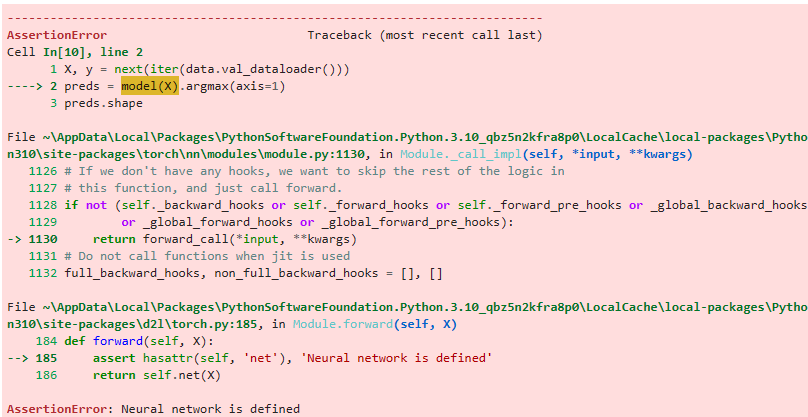
X, y = next(iter(data.val_dataloader()))
preds = model(X).argmax(axis=1)
preds.shape

위의 코드는 검증 데이터셋에서 첫 번째 배치를 가져와서 모델에 입력으로 전달하고, 모델의 예측 결과를 저장하는 과정을 나타냅니다. 코드를 한 줄씩 설명해드리겠습니다.

1. X, y = next(iter(data.val_dataloader())): data.val_dataloader()를 통해 검증 데이터셋의 첫 번째 배치를 가져옵니다. next(iter(...))를 사용하여 이터레이터에서 다음 값을 가져옵니다. X는 입력 데이터를, y는 해당 데이터의 정답 레이블을 나타냅니다.
2. preds = model(X).argmax(axis=1): 모델 model에 입력 데이터 X를 전달하여 예측 결과를 얻습니다. model(X)는 입력 데이터에 대한 예측값을 반환합니다. argmax(axis=1)를 사용하여 각 데이터 포인트마다 가장 큰 값의 인덱스를 구합니다. 따라서 preds에는 각 데이터 포인트의 예측된 클래스 인덱스가 저장됩니다.
3. preds.shape: preds의 형태(shape)를 확인합니다. 이는 예측된 클래스 인덱스의 개수를 나타냅니다.

결과적으로, 위의 코드는 검증 데이터셋에서 첫 번째 배치를 사용하여 모델의 예측 결과를 얻고, 예측된 클래스 인덱스를 preds에 저장합니다. preds의 형태(shape)를 확인하여 예측된 클래스 인덱스의 개수를 알 수 있습니다.

Local에서 돌린 결과

CoLab에서 돌린 결과

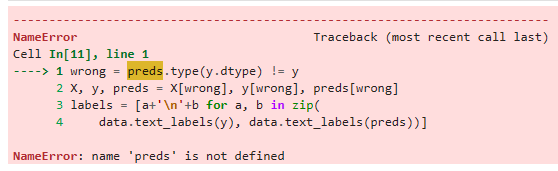
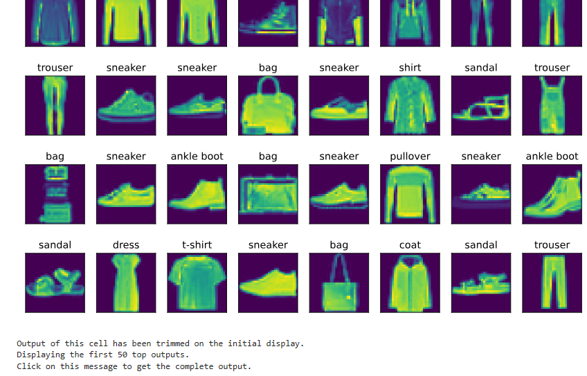
We are more interested in the images we label incorrectly. We visualize them by comparing their actual labels (first line of text output) with the predictions from the model (second line of text output).

우리는 잘못 라벨을 붙인 이미지에 더 관심이 있습니다. 실제 레이블(텍스트 출력의 첫 번째 줄)과 모델의 예측(텍스트 출력의 두 번째 줄)을 비교하여 시각화합니다.

wrong = preds.type(y.dtype) != y
X, y, preds = X[wrong], y[wrong], preds[wrong]
labels = [a+'\n'+b for a, b in zip(
    data.text_labels(y), data.text_labels(preds))]
data.visualize([X, y], labels=labels)

위의 코드는 잘못 예측된 샘플들을 시각화하는 과정을 나타냅니다. 코드를 한 줄씩 설명해드리겠습니다.

1. wrong = preds.type(y.dtype) != y: 모델의 예측값 preds와 정답 레이블 y를 비교하여 잘못 예측된 샘플을 식별합니다. preds.type(y.dtype)를 사용하여 preds의 데이터 타입을 y와 일치시키고, != 연산자를 사용하여 예측값과 정답 레이블을 비교합니다. 이 결과를 wrong에 저장합니다.
2. X, y, preds = X[wrong], y[wrong], preds[wrong]: 잘못 예측된 샘플에 대한 입력 데이터 X, 정답 레이블 y, 예측값 preds를 추출하여 각각 X[wrong], y[wrong], preds[wrong]에 저장합니다. 이렇게 하면 잘못 예측된 샘플들만 남게 됩니다.
3. labels = [a+'\n'+b for a, b in zip(data.text_labels(y), data.text_labels(preds))]: 잘못 예측된 샘플들에 대한 정답 레이블 y와 예측값 preds를 사용하여 레이블 텍스트를 생성합니다. data.text_labels(y)와 data.text_labels(preds)를 순회하면서 정답 레이블과 예측값을 합쳐서 하나의 문자열로 만들고, 이를 labels 리스트에 저장합니다.
4. data.visualize([X, y], labels=labels): 입력 데이터 X와 정답 레이블 y를 사용하여 시각화를 수행합니다. labels를 추가적인 인자로 전달하여 각 샘플의 레이블을 텍스트로 표시합니다.

결과적으로, 위의 코드는 잘못 예측된 샘플들을 추출하고, 해당 샘플들의 입력 데이터와 레이블을 시각화하여 표시합니다. 또한, 정답 레이블과 예측값을 텍스트로 표시하여 시각화에 추가합니다.

Local에서 돌린 결과

CoLab에서 돌린 결과

4.4.6. Summary

By now we are starting to get some experience with solving linear regression and classification problems. With it, we have reached what would arguably be the state of the art of 1960-1970s of statistical modeling. In the next section, we will show you how to leverage deep learning frameworks to implement this model much more efficiently.

이제 우리는 선형 회귀 및 분류 문제를 해결하는 경험을 쌓기 시작했습니다. 이를 통해 우리는 1960-1970년대의 통계 모델링 기술 수준에 도달했습니다. 다음 섹션에서는 딥 러닝 프레임워크를 활용하여 이 모델을 훨씬 더 효율적으로 구현하는 방법을 보여줍니다.

4.4.7. Exercises

https://d2l.ai/chapter_linear-classification/classification.html

4.3. The Base Classification Model

You may have noticed that the implementations from scratch and the concise implementation using framework functionality were quite similar in the case of regression. The same is true for classification. Since many models in this book deal with classification, it is worth adding functionalities to support this setting specifically. This section provides a base class for classification models to simplify future code.

처음부터 구현하는 것과 프레임워크 기능을 사용하는 간결한 구현이 회귀의 경우 상당히 유사하다는 것을 알아차렸을 것입니다. 분류도 마찬가지입니다. 이 책의 많은 모델이 분류를 다루기 때문에 이 설정을 구체적으로 지원하는 기능을 추가할 가치가 있습니다. 이 섹션에서는 향후 코드를 단순화하기 위한 분류 모델의 기본 클래스를 제공합니다.

import torch
from d2l import torch as d2l

위 코드는 torch와 d2l을 import 하는 부분입니다.

torch는 PyTorch의 메인 패키지로, 다양한 텐서 연산과 신경망 구성 요소를 제공합니다. d2l은 Dive into Deep Learning(D2L) 도서의 예제 코드와 유틸리티 함수를 제공하는 패키지입니다.

이 코드는 PyTorch와 D2L 패키지를 가져와서 해당 패키지의 기능을 사용할 수 있도록 준비하는 단계입니다. 이후 코드에서는 PyTorch와 D2L의 함수와 클래스를 사용하여 딥러닝 모델을 구축하고 학습하는 등의 작업을 수행할 수 있습니다.

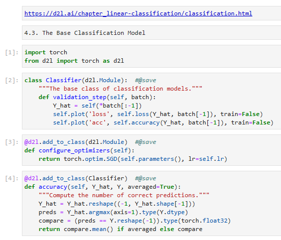
4.3.1. The Classifier Class

We define the Classifier class below. In the validation_step we report both the loss value and the classification accuracy on a validation batch. We draw an update for every num_val_batches batches. This has the benefit of generating the averaged loss and accuracy on the whole validation data. These average numbers are not exactly correct if the last batch contains fewer examples, but we ignore this minor difference to keep the code simple.

아래에서 Classifier 클래스를 정의합니다. validation_step에서 검증 배치에 대한 손실 값과 분류 정확도를 모두 보고합니다. 모든 num_val_batches 배치에 대해 업데이트를 그립니다. 이는 전체 유효성 검사 데이터에 대한 평균 손실 및 정확도를 생성하는 이점이 있습니다. 마지막 배치에 더 적은 예가 포함된 경우 이러한 평균 수치는 정확히 정확하지 않지만 코드를 단순하게 유지하기 위해 이 사소한 차이를 무시합니다.

class Classifier(d2l.Module):  #@save
    """The base class of classification models."""
    def validation_step(self, batch):
        Y_hat = self(*batch[:-1])
        self.plot('loss', self.loss(Y_hat, batch[-1]), train=False)
        self.plot('acc', self.accuracy(Y_hat, batch[-1]), train=False)

위 코드는 Classifier라는 클래스를 정의하는 부분입니다.

Classifier는 분류 모델의 기본 클래스로 사용되며, d2l.Module을 상속받습니다. d2l.Module은 Dive into Deep Learning(D2L) 도서에서 제공하는 모듈을 확장한 클래스로, 신경망 모델을 정의하고 학습하는 데 도움이 되는 다양한 기능을 제공합니다.

Classifier 클래스는 validation_step 메서드를 가지고 있습니다. 이 메서드는 검증 단계(validation step)에서 수행되는 작업을 정의합니다. 입력으로는 batch가 주어지며, Y_hat = self(*batch[:-1]) 코드는 모델에 batch의 입력값을 전달하여 예측값 Y_hat을 얻습니다. 그리고 self.plot 메서드를 사용하여 손실값(loss)과 정확도(acc)를 시각화합니다. self.loss와 self.accuracy는 모델에서 정의된 손실 함수와 정확도 함수를 호출하여 값을 계산하는 역할을 합니다.

이 코드는 분류 모델의 기본 클래스를 정의하고, 검증 단계에서 손실과 정확도를 기록하여 모니터링하는 기능을 제공합니다. 이후 이 클래스를 상속받아 실제 분류 모델을 정의하고 학습할 수 있습니다.

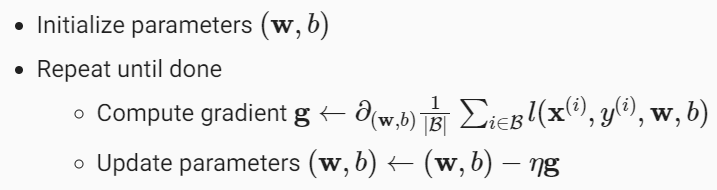
By default we use a stochastic gradient descent optimizer, operating on minibatches, just as we did in the context of linear regression.

기본적으로 우리는 선형 회귀의 맥락에서 했던 것처럼 미니배치에서 작동하는 확률적 경사 하강 최적화 프로그램을 사용합니다.

@d2l.add_to_class(d2l.Module)  #@save
def configure_optimizers(self):
    return torch.optim.SGD(self.parameters(), lr=self.lr)

위 코드는 configure_optimizers라는 메서드를 d2l.Module 클래스에 추가하는 부분입니다.

configure_optimizers 메서드는 최적화기(optimizer)를 설정하는 역할을 합니다. 이 메서드는 현재 모델의 파라미터와 학습률(lr)을 사용하여 torch.optim.SGD를 생성하고 반환합니다. 이 경우, torch.optim.SGD는 확률적 경사 하강법(SGD)을 사용하여 모델의 파라미터를 최적화하는 최적화기입니다.

@d2l.add_to_class(d2l.Module) 데코레이터는 configure_optimizers 메서드를 d2l.Module 클래스에 추가하여 해당 클래스의 모든 인스턴스에서 사용할 수 있도록 합니다. 이렇게 하면 모델의 파라미터를 최적화하기 위한 옵티마이저를 쉽게 구성할 수 있습니다.

따라서, 이 코드는 d2l.Module 클래스에 configure_optimizers 메서드를 추가하여 옵티마이저를 설정하는 기능을 제공합니다. 이후 모델을 생성하고 학습할 때 이 메서드를 호출하여 옵티마이저를 구성하고 사용할 수 있습니다.

4.3.2. Accuracy

Given the predicted probability distribution y_hat, we typically choose the class with the highest predicted probability whenever we must output a hard prediction. Indeed, many applications require that we make a choice. For instance, Gmail must categorize an email into “Primary”, “Social”, “Updates”, “Forums”, or “Spam”. It might estimate probabilities internally, but at the end of the day it has to choose one among the classes.

예측 확률 분포 y_hat이 주어지면 일반적으로 어려운 예측을 출력해야 할 때마다 예측 확률이 가장 높은 클래스를 선택합니다. 실제로 많은 애플리케이션에서 선택을 요구합니다. 예를 들어 Gmail은 이메일을 "기본", "소셜", "업데이트", "포럼" 또는 "스팸"으로 분류해야 합니다. 내부적으로 확률을 추정할 수 있지만 결국 클래스 중에서 하나를 선택해야 합니다.

When predictions are consistent with the label class y, they are correct. The classification accuracy is the fraction of all predictions that are correct. Although it can be difficult to optimize accuracy directly (it is not differentiable), it is often the performance measure that we care about the most. It is often the relevant quantity in benchmarks. As such, we will nearly always report it when training classifiers.

예측이 레이블 클래스 y와 일치하면 올바른 것입니다. 분류 정확도는 올바른 모든 예측의 비율입니다. 정확도를 직접 최적화하는 것은 어려울 수 있지만(미분 가능하지 않음) 종종 우리가 가장 중요하게 생각하는 성능 측정입니다. 종종 벤치마크에서 관련 수량입니다. 따라서 분류기를 교육할 때 거의 항상 보고합니다.

Accuracy is computed as follows. First, if y_hat is a matrix, we assume that the second dimension stores prediction scores for each class. We use argmax to obtain the predicted class by the index for the largest entry in each row. Then we compare the predicted class with the ground-truth y elementwise. Since the equality operator == is sensitive to data types, we convert y_hat’s data type to match that of y. The result is a tensor containing entries of 0 (false) and 1 (true). Taking the sum yields the number of correct predictions.

정확도는 다음과 같이 계산됩니다. 첫째, y_hat이 행렬인 경우 두 번째 차원이 각 클래스에 대한 예측 점수를 저장한다고 가정합니다. argmax를 사용하여 각 행에서 가장 큰 항목에 대한 인덱스로 예측 클래스를 얻습니다. 그런 다음 예측된 클래스를 ground-truth y와 요소별로 비교합니다. 항등 연산자 ==는 데이터 유형에 민감하므로 y_hat의 데이터 유형을 y의 데이터 유형과 일치하도록 변환합니다. 결과는 0(거짓) 및 1(참) 항목을 포함하는 텐서입니다. 합계를 취하면 올바른 예측의 수가 산출됩니다.

@d2l.add_to_class(Classifier)  #@save
def accuracy(self, Y_hat, Y, averaged=True):
    """Compute the number of correct predictions."""
    Y_hat = Y_hat.reshape((-1, Y_hat.shape[-1]))
    preds = Y_hat.argmax(axis=1).type(Y.dtype)
    compare = (preds == Y.reshape(-1)).type(torch.float32)
    return compare.mean() if averaged else compare

위 코드는 accuracy라는 메서드를 Classifier 클래스에 추가하는 부분입니다.

accuracy 메서드는 예측값(Y_hat)과 실제값(Y)을 비교하여 정확도를 계산하는 역할을 합니다. 이 메서드는 예측값(Y_hat)을 평탄화(flatten)한 후 가장 높은 확률을 가진 클래스로 예측하고, 이를 실제값(Y)와 비교하여 정확한 예측의 개수를 계산합니다.

@d2l.add_to_class(Classifier) 데코레이터는 accuracy 메서드를 Classifier 클래스에 추가하여 해당 클래스의 모든 인스턴스에서 사용할 수 있도록 합니다. 이렇게 하면 분류 모델에서 정확도를 쉽게 계산할 수 있습니다.

따라서, 이 코드는 Classifier 클래스에 accuracy 메서드를 추가하여 모델의 정확도를 계산하는 기능을 제공합니다. 이후 모델을 생성하고 학습 또는 평가할 때 이 메서드를 호출하여 정확도를 계산할 수 있습니다.

1. @d2l.add_to_class(Classifier): 이는 다음의 메서드를 Classifier 클래스에 추가하는 데코레이터입니다.
2. def accuracy(self, Y_hat, Y, averaged=True):: 이는 accuracy 메서드를 정의합니다. 이 메서드는 세 개의 인자를 받습니다: Y_hat (예측값), Y (실제값) 그리고 선택적으로 사용되는 averaged 플래그입니다.
3. Y_hat = Y_hat.reshape((-1, Y_hat.shape[-1])): 이 줄은 예측값 Y_hat의 모양을 (배치 크기, 클래스 개수)로 변경합니다. 이는 텐서를 첫 번째 차원을 따라 펼치고 두 번째 차원은 그대로 유지합니다.
4. preds = Y_hat.argmax(axis=1).type(Y.dtype): 이는 Y_hat의 두 번째 차원(클래스 확률)을 따라 최댓값의 인덱스를 찾아 예측된 클래스를 계산합니다. 결과로 나오는 preds 텐서는 예측된 클래스 인덱스를 담고 있으며, 이를 Y와 동일한 데이터 타입으로 변환합니다.
5. compare = (preds == Y.reshape(-1)).type(torch.float32): 이 줄은 Y를 (배치 크기,) 모양으로 변경한 후, 예측된 클래스(preds)와 실제 클래스(Y)를 비교합니다. 결과로는 예측이 올바른지 여부를 나타내는 불리언 값으로 이루어진 텐서가 생성됩니다. 이를 torch.float32 데이터 타입으로 변환합니다.
6. return compare.mean() if averaged else compare: 이 줄은 compare 텐서의 평균을 계산하여 정확도를 반환합니다. 만약 averaged가 True인 경우, 평균 정확도를 반환합니다. averaged가 False인 경우, 정확한 예측의 원시 텐서를 반환합니다. 평균 정확도는 배치 내 전체 예측의 올바른 예측 비율을 나타냅니다.

이 코드는 Classifier 클래스에 accuracy 메서드를 추가하여 모델의 예측의 정확도를 계산합니다. 메서드는 averaged 플래그에 따라 평균화된 정확도와 평균화되지 않은 정확도를 모두 계산할 수 있는 유연성을 가지고 있습니다.

local에서 실행한 화면

4.3.3. Summary

Classification is a sufficiently common problem that it warrants its own convenience functions. Of central importance in classification is the accuracy of the classifier. Note that while we often care primarily about accuracy, we train classifiers to optimize a variety of other objectives for statistical and computational reasons. However, regardless of which loss function was minimized during training, it is useful to have a convenience method for assessing the accuracy of our classifier empirically.

분류는 자체 편의 기능을 보장하는 충분히 일반적인 문제입니다. 분류에서 가장 중요한 것은 분류기의 정확도입니다. 주로 정확도에 관심을 두는 경우가 많지만 통계 및 계산상의 이유로 다양한 다른 목표를 최적화하도록 분류기를 훈련합니다. 그러나 훈련 중에 어떤 손실 함수가 최소화되었는지에 관계없이 경험적으로 분류기의 정확도를 평가할 수 있는 편리한 방법이 있으면 유용합니다.

4.3.4. Exercises

https://d2l.ai/chapter_linear-classification/image-classification-dataset.html

4.2. The Image Classification Dataset

One of the widely used dataset for image classification is the MNIST dataset (LeCun et al., 1998) of handwritten digits. At the time of its release in the 1990s it posed a formidable challenge to most machine learning algorithms, consisting of 60,000 images of 28×28 pixels resolution (plus a test dataset of 10,000 images). To put things into perspective, at the time, a Sun SPARCStation 5 with a whopping 64MB of RAM and a blistering 5 MFLOPs was considered state of the art equipment for machine learning at AT&T Bell Laboratories in 1995. Achieving high accuracy on digit recognition was a key component in automating letter sorting for the USPS in the 1990s. Deep networks such as LeNet-5 (LeCun et al., 1995), support vector machines with invariances (Schölkopf et al., 1996), and tangent distance classifiers (Simard et al., 1998) all allowed to reach error rates below 1%.

 

이미지 분류를 위해 널리 사용되는 데이터 세트 중 하나는 손으로 쓴 숫자의 MNIST 데이터 세트(LeCun et al., 1998)입니다. 1990년대 출시 당시에는 픽셀 해상도의 60,000개 이미지(및 10,000개 이미지의 테스트 데이터 세트)로 구성된 대부분의 기계 학습 알고리즘에 엄청난 도전 과제였습니다. 1995년 AT&T Bell Laboratories에서는 당시 엄청난 64MB의 RAM과 5개의 MFLOP를 탑재한 Sun SPARCStation 5가 기계 학습을 위한 최첨단 장비로 간주되었습니다. 숫자 인식에서 높은 정확도를 달성하는 것은 1990년대 USPS의 자동 문자 정렬의 핵심 구성 요소. LeNet-5(LeCun et al., 1995), 불변성이 있는 지원 벡터 머신(Schölkopf et al., 1996), 접선 거리 분류기(Simard et al., 1998)와 같은 심층 네트워크는 모두 1% 미만의 오류율에 도달하도록 허용되었습니다. 

 

 

For over a decade, MNIST served as the point of reference for comparing machine learning algorithms. While it had a good run as a benchmark dataset, even simple models by today’s standards achieve classification accuracy over 95%, making it unsuitable for distinguishing between stronger models and weaker ones. Even more so, the dataset allows for very high levels of accuracy, not typically seen in many classification problems. This skewed algorithmic development towards specific families of algorithms that can take advantage of clean datasets, such as active set methods and boundary-seeking active set algorithms. Today, MNIST serves as more of sanity checks than as a benchmark. ImageNet (Deng et al., 2009) poses a much more relevant challenge. Unfortunately, ImageNet is too large for many of the examples and illustrations in this book, as it would take too long to train to make the examples interactive. As a substitute we will focus our discussion in the coming sections on the qualitatively similar, but much smaller Fashion-MNIST dataset (Xiao et al., 2017), which was released in 2017. It contains images of 10 categories of clothing at 28×28 pixels resolution.

 

 

10년 넘게 MNIST는 기계 학습 알고리즘을 비교하기 위한 기준점 역할을 했습니다. 벤치마크 데이터 세트로 잘 실행되었지만 오늘날의 표준에 따른 단순한 모델도 95% 이상의 분류 정확도를 달성하여 더 강한 모델과 약한 모델을 구별하는 데 적합하지 않습니다. 더욱이 데이터 세트는 일반적으로 많은 분류 문제에서 볼 수 없는 매우 높은 수준의 정확도를 허용합니다. 이러한 왜곡된 알고리즘 개발은 활성 세트 방법 및 경계 탐색 활성 세트 알고리즘과 같은 클린 데이터 세트를 활용할 수 있는 특정 알고리즘 제품군으로 향합니다. 오늘날 MNIST는 벤치마크가 아닌 온전성 검사 역할을 합니다. ImageNet(Deng et al., 2009)은 훨씬 더 적절한 문제를 제기합니다. 불행하게도 ImageNet은 이 책의 많은 예제와 삽화에 비해 너무 큽니다. 예제를 대화형으로 만들려면 훈련하는 데 너무 오래 걸리기 때문입니다. 그 대안으로 우리는 2017년에 출시된 질적으로 유사하지만 훨씬 더 작은 Fashion-MNIST 데이터 세트(Xiao et al., 2017)에 대해 다음 섹션에서 논의에 집중할 것입니다. 여기에는 "28 × 28" 픽셀 해상도의 10가지 의류 카테고리 이미지가 포함되어 있습니다.

 

 

%matplotlib inline
import time
import torch
import torchvision
from torchvision import transforms
from d2l import torch as d2l

d2l.use_svg_display()

 

Local에서 실행한 결과

 

 

 

위 코드는 PyTorch와 함께 딥러닝 라이브러리인 d2l (Dive into Deep Learning)을 사용하기 위한 환경을 설정하는 데 사용됩니다. 코드를 단계별로 살펴보겠습니다:

1. %matplotlib inline: 이는 주피터 노트북의 매직 명령어로, matplotlib 그래프를 노트북 안에서 직접 표시할 수 있게 합니다.
2. import time: time 모듈을 가져옵니다. 이 모듈은 시간과 관련된 작업을 수행하는 함수들을 제공합니다.
3. import torch: PyTorch 라이브러리를 가져옵니다. PyTorch는 인기 있는 오픈 소스 딥러닝 프레임워크입니다.
4. import torchvision: torchvision 라이브러리를 가져옵니다. torchvision은 컴퓨터 비전 작업을 위한 사전 훈련된 모델과 데이터셋을 제공합니다.
5. from torchvision import transforms: torchvision에서 transforms 모듈을 가져옵니다. 이 모듈은 일반적인 이미지 변환 기능을 제공합니다.
6. from d2l import torch as d2l: d2l 라이브러리에서 torch 모듈을 가져옵니다. d2l은 PyTorch와 함께 작업하기 위한 다양한 유틸리티와 함수를 제공하는 딥러닝 라이브러리입니다.
7. d2l.use_svg_display(): 이는 d2l 라이브러리의 함수 호출로, 그래프의 표시 형식을 SVG (Scalable Vector Graphics) 형식으로 설정합니다. 이렇게 함으로써 d2l이 생성한 그래프가 주피터 노트북에서 올바르게 표시됩니다.

이 코드 세그먼트는 d2l 라이브러리를 PyTorch와 함께 사용하기 위한 필요한 라이브러리와 설정을 설정합니다. 이를 통해 딥러닝 모델과 데이터셋을 사용할 수 있게 됩니다.

 

 

4.2.1. Loading the Dataset

 

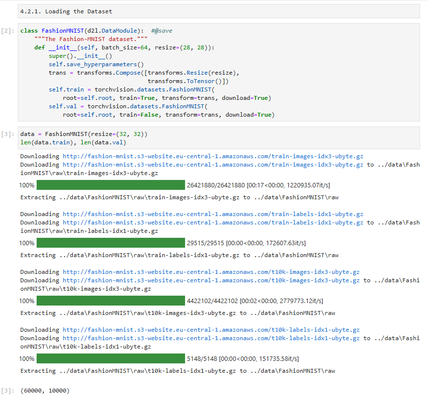
Since it is such a frequently used dataset, all major frameworks provide preprocessed versions of it. We can download and read the Fashion-MNIST dataset into memory using built-in framework utilities.

 

자주 사용되는 데이터 세트이기 때문에 모든 주요 프레임워크는 전처리된 버전을 제공합니다. 내장된 프레임워크 유틸리티를 사용하여 Fashion-MNIST 데이터 세트를 다운로드하고 메모리로 읽을 수 있습니다.

class FashionMNIST(d2l.DataModule):  #@save
    """The Fashion-MNIST dataset."""
    def __init__(self, batch_size=64, resize=(28, 28)):
        super().__init__()
        self.save_hyperparameters()
        trans = transforms.Compose([transforms.Resize(resize),
                                    transforms.ToTensor()])
        self.train = torchvision.datasets.FashionMNIST(
            root=self.root, train=True, transform=trans, download=True)
        self.val = torchvision.datasets.FashionMNIST(
            root=self.root, train=False, transform=trans, download=True)

위 코드는 Fashion-MNIST 데이터셋을 사용하기 위한 FashionMNIST 클래스를 정의하는 부분입니다. 코드를 한 줄씩 살펴보겠습니다.

• FashionMNIST 클래스는 d2l.DataModule을 상속받아 Fashion-MNIST 데이터셋을 사용할 수 있도록 합니다.
• __init__ 메서드는 클래스의 생성자입니다. batch_size와 resize를 매개변수로 받습니다.
• super().__init__()은 상위 클래스인 d2l.DataModule의 생성자를 호출합니다.
• self.save_hyperparameters()는 현재 클래스의 하이퍼파라미터를 저장합니다.
• trans는 데이터 변환을 위한 transforms.Compose 객체입니다. transforms.Resize(resize)는 이미지 크기를 resize 크기로 조정하는 변환을 수행하고, transforms.ToTensor()는 이미지를 텐서로 변환하는 변환을 수행합니다.
• self.train은 학습 데이터셋을 나타내는 torchvision.datasets.FashionMNIST 객체입니다. root는 데이터셋을 저장할 디렉토리를 의미하며, train=True는 학습 데이터셋을 로드하라는 의미입니다. transform은 데이터 변환을 적용하는 것을 의미하고, download=True는 데이터셋이 로컬에 없을 경우 다운로드하도록 지정합니다.
• self.val은 검증 데이터셋을 나타내는 torchvision.datasets.FashionMNIST 객체입니다. train=False로 설정하여 검증 데이터셋을 로드하도록 지정합니다.

이 코드는 Fashion-MNIST 데이터셋을 사용하기 위해 필요한 클래스와 데이터 변환을 초기화하는 부분입니다. 이를 통해 학습 데이터셋과 검증 데이터셋을 사용할 수 있습니다.

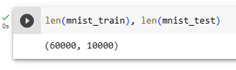
Fashion-MNIST consists of images from 10 categories, each represented by 6,000 images in the training dataset and by 1,000 in the test dataset. A test dataset is used for evaluating model performance (it must not be used for training). Consequently the training set and the test set contain 60,000 and 10,000 images, respectively.

Fashion-MNIST는 10개 범주의 이미지로 구성되며 각 범주는 훈련 데이터 세트에서 6,000개의 이미지로, 테스트 데이터 세트에서 1,000개로 표시됩니다. 테스트 데이터 세트는 모델 성능을 평가하는 데 사용됩니다(학습에 사용해서는 안 됨). 결과적으로 훈련 세트와 테스트 세트에는 각각 60,000개와 10,000개의 이미지가 포함됩니다.

data = FashionMNIST(resize=(32, 32))
len(data.train), len(data.val)

Local에서 실행한 결과.

위 코드는 FashionMNIST 데이터셋을 생성하고, 학습 데이터셋과 검증 데이터셋의 길이를 확인하는 부분입니다. 코드를 한 줄씩 살펴보겠습니다.

• data = FashionMNIST(resize=(32, 32))는 FashionMNIST 클래스의 객체를 생성하고, resize 매개변수를 (32, 32)로 설정하여 이미지 크기를 32x32로 조정합니다.
• len(data.train), len(data.val)은 data.train과 data.val의 길이를 확인하는 코드입니다. len(data.train)은 학습 데이터셋의 샘플 수를 반환하고, len(data.val)은 검증 데이터셋의 샘플 수를 반환합니다.

이 코드는 FashionMNIST 데이터셋 객체를 생성하고, 학습 데이터셋과 검증 데이터셋의 길이를 확인하는 부분입니다.

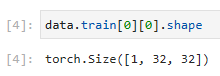
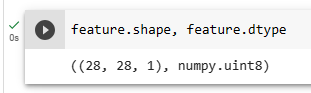
The images are grayscale and upscaled to 32×32 pixels in resolution above. This is similar to the original MNIST dataset which consisted of (binary) black and white images. Note, though, that most modern image data which has 3 channels (red, green, blue) and hyperspectral images which can have in excess of 100 channels (the HyMap sensor has 126 channels). By convention we store image as a c×ℎ×w tensor, where c is the number of color channels, ℎ is the height and w is the width.

이미지는 그레이스케일이며 위의 해상도에서 32×32 픽셀로 업스케일됩니다. 이것은 (바이너리) 흑백 이미지로 구성된 원본 MNIST 데이터 세트와 유사합니다. 그러나 3개 채널(빨간색, 녹색, 파란색)이 있는 대부분의 최신 이미지 데이터와 100개 이상의 채널(HyMap 센서에는 126개 채널이 있음)을 가질 수 있는 초분광 이미지가 있습니다. 관례적으로 우리는 이미지를 c×ℎ×w 텐서로 저장합니다. 여기서 c는 색상 채널 수, ℎ는 높이, w는 너비입니다.

data.train[0][0].shape

이 코드는 FashionMNIST 학습 데이터셋의 첫 번째 샘플의 이미지의 형태(shape)를 확인하는 부분입니다.

• data.train[0]은 학습 데이터셋의 첫 번째 샘플을 의미합니다. 이 샘플은 튜플 형태로 구성되어 있으며, 첫 번째 요소는 이미지를 나타냅니다.
• data.train[0][0]은 첫 번째 샘플의 이미지를 의미합니다.
• .shape는 이미지의 형태(shape)를 반환하는 속성(attribute)입니다. 이를 통해 이미지의 차원과 크기를 확인할 수 있습니다.

따라서 위의 코드는 FashionMNIST 학습 데이터셋의 첫 번째 샘플의 이미지의 형태(shape)를 확인하는 부분입니다.

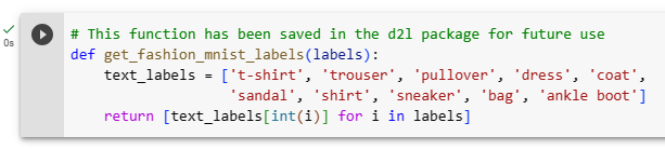
The categories of Fashion-MNIST have human-understandable names. The following convenience method converts between numeric labels and their names.

Fashion-MNIST의 범주에는 사람이 이해할 수 있는 이름이 있습니다. 다음 편의 메서드는 숫자 레이블과 이름 사이를 변환합니다.

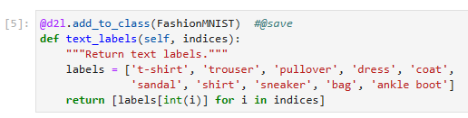
@d2l.add_to_class(FashionMNIST)  #@save
def text_labels(self, indices):
    """Return text labels."""
    labels = ['t-shirt', 'trouser', 'pullover', 'dress', 'coat',
              'sandal', 'shirt', 'sneaker', 'bag', 'ankle boot']
    return [labels[int(i)] for i in indices]

이 코드는 FashionMNIST 클래스에 text_labels 메서드를 추가하는 부분입니다. 이 메서드는 주어진 인덱스에 해당하는 레이블을 텍스트 형태로 반환합니다. 코드를 한 줄씩 살펴보겠습니다.

• @d2l.add_to_class(FashionMNIST)는 FashionMNIST 클래스에 text_labels 메서드를 추가하기 위한 데코레이터(decorator)입니다. 이를 통해 클래스 외부에서 해당 메서드를 정의할 수 있습니다.
• def text_labels(self, indices):는 text_labels 메서드를 정의하는 부분입니다. 이 메서드는 self와 indices를 매개변수로 받습니다.
• labels는 Fashion-MNIST 클래스에 대응하는 레이블을 나타내는 문자열 리스트입니다.
• [labels[int(i)] for i in indices]는 주어진 인덱스에 해당하는 레이블을 텍스트 형태로 반환하는 코드입니다. indices는 인덱스들의 리스트이며, int(i)를 통해 각 인덱스를 정수로 변환한 후 labels에서 해당하는 레이블을 가져옵니다.

이 코드는 FashionMNIST 클래스에 text_labels 메서드를 추가하여 주어진 인덱스에 해당하는 레이블을 텍스트 형태로 반환할 수 있도록 합니다.

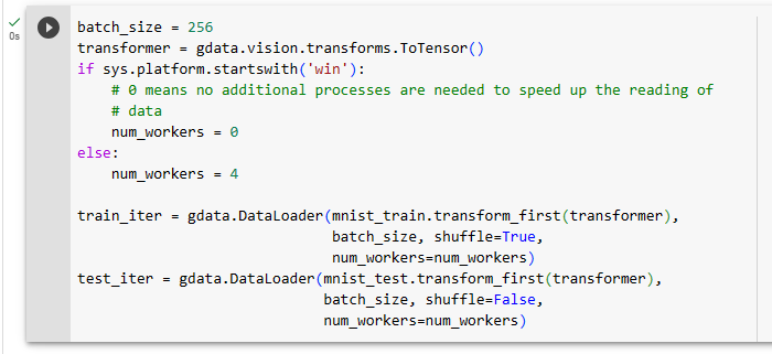
4.2.2. Reading a Minibatch

To make our life easier when reading from the training and test sets, we use the built-in data iterator rather than creating one from scratch. Recall that at each iteration, a data iterator reads a minibatch of data with size batch_size. We also randomly shuffle the examples for the training data iterator.

학습 및 테스트 세트에서 읽을 때 삶을 더 쉽게 만들기 위해 처음부터 새로 만드는 대신 내장된 데이터 반복자를 사용합니다. 각 반복에서 데이터 반복자는 크기가 batch_size인 데이터의 미니 배치를 읽습니다. 또한 교육 데이터 반복자에 대한 예제를 무작위로 섞습니다.

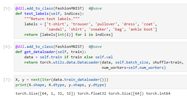
@d2l.add_to_class(FashionMNIST)  #@save
def get_dataloader(self, train):
    data = self.train if train else self.val
    return torch.utils.data.DataLoader(data, self.batch_size, shuffle=train,
                                       num_workers=self.num_workers)

위 코드는 FashionMNIST 클래스에 get_dataloader 메서드를 추가하는 부분입니다. 이 메서드는 주어진 train 매개변수에 따라 학습 데이터셋 또는 검증 데이터셋에 대한 데이터 로더(DataLoader)를 반환합니다. 코드를 한 줄씩 살펴보겠습니다.

• @d2l.add_to_class(FashionMNIST)는 FashionMNIST 클래스에 get_dataloader 메서드를 추가하기 위한 데코레이터(decorator)입니다.
• def get_dataloader(self, train):는 get_dataloader 메서드를 정의하는 부분입니다. 이 메서드는 self와 train을 매개변수로 받습니다.
• data = self.train if train else self.val는 train이 True일 경우 학습 데이터셋(self.train)을, 그렇지 않은 경우 검증 데이터셋(self.val)을 선택하여 data 변수에 할당합니다.
• torch.utils.data.DataLoader(data, self.batch_size, shuffle=train, num_workers=self.num_workers)는 데이터 로더(DataLoader) 객체를 생성합니다. data는 로딩할 데이터셋을 나타내며, self.batch_size는 배치 크기를, shuffle=train은 학습 데이터셋인 경우에는 데이터를 섞어서 로드하도록 설정합니다. num_workers=self.num_workers는 데이터를 로드할 때 사용할 워커(worker)의 수를 나타냅니다.

이 코드는 FashionMNIST 클래스에 get_dataloader 메서드를 추가하여 학습 데이터셋 또는 검증 데이터셋에 대한 데이터 로더를 반환할 수 있도록 합니다.

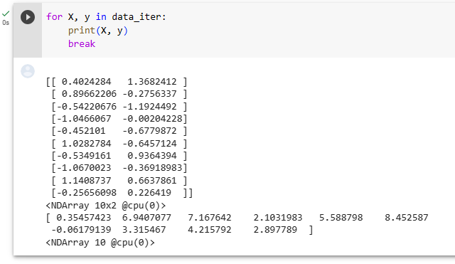
To see how this works, let’s load a minibatch of images by invoking the train_dataloader method. It contains 64 images.

작동 방식을 확인하기 위해 train_dataloader 메서드를 호출하여 이미지의 미니 배치를 로드해 보겠습니다. 64개의 이미지가 포함되어 있습니다.

X, y = next(iter(data.train_dataloader()))
print(X.shape, X.dtype, y.shape, y.dtype)

위 코드는 데이터셋의 첫 번째 배치를 가져와서 배치의 형태(shape)와 데이터 타입(dtype)을 출력하는 부분입니다.

• next(iter(data.train_dataloader()))는 데이터 로더(data.train_dataloader())에서 첫 번째 배치를 가져오는 것을 의미합니다. iter() 함수를 통해 데이터 로더를 이터레이터로 변환하고, next() 함수를 호출하여 첫 번째 배치를 가져옵니다.
• X, y = next(iter(data.train_dataloader()))는 가져온 첫 번째 배치를 X와 y 변수에 할당합니다. 여기서 X는 입력 데이터를, y는 해당하는 타깃(label) 데이터를 나타냅니다.
• print(X.shape, X.dtype, y.shape, y.dtype)는 X와 y의 형태(shape)와 데이터 타입(dtype)을 출력합니다. .shape은 배열의 차원과 크기를 나타내는 속성(attribute)이며, .dtype은 배열의 데이터 타입을 나타내는 속성입니다.

따라서 위의 코드는 데이터셋의 첫 번째 배치를 가져와서 해당 배치의 형태와 데이터 타입을 출력하는 부분입니다.

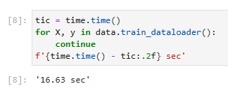
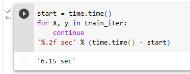
Let’s look at the time it takes to read the images. Even though it is a built-in loader, it is not blazingly fast. Nonetheless, this is sufficient since processing images with a deep network takes quite a bit longer. Hence it is good enough that training a network will not be IO constrained.

이미지를 읽는 데 걸리는 시간을 살펴보겠습니다. 빌트인 로더임에도 불구하고 엄청나게 빠르지는 않습니다. 그럼에도 불구하고 딥 네트워크로 이미지를 처리하는 데 시간이 꽤 오래 걸리므로 이 정도면 충분합니다. 따라서 네트워크 교육이 IO 제약을 받지 않는 것으로 충분합니다.

tic = time.time()
for X, y in data.train_dataloader():
    continue
f'{time.time() - tic:.2f} sec'

위 코드는 학습 데이터셋을 반복(iterate)하면서 각 배치의 처리 시간을 측정하는 부분입니다.

• tic = time.time()은 현재 시간을 기록하는 부분으로, 시간 측정의 시작점을 나타냅니다.
• for X, y in data.train_dataloader():는 학습 데이터셋의 데이터 로더를 이용하여 배치 단위로 데이터를 가져오는 반복문입니다. X는 입력 데이터를, y는 해당하는 타깃(label) 데이터를 나타냅니다. 여기서 continue 문은 아무 작업도 수행하지 않고 다음 반복으로 진행하도록 합니다.
• f'{time.time() - tic:.2f} sec'은 시간 측정이 끝난 후에 경과 시간을 계산하여 소수점 둘째 자리까지 문자열로 반환합니다. {time.time() - tic:.2f}은 경과 시간을 소수점 둘째 자리까지 표시하도록 지정한 것이며, ' sec'는 문자열 " sec"를 추가하여 최종 문자열을 생성합니다.

따라서 위의 코드는 학습 데이터셋의 모든 배치를 순회하면서 처리 시간을 측정하고, 총 소요 시간을 출력하는 부분입니다. 출력 결과는 경과 시간이 소수점 둘째 자리까지 표시된 문자열로 나타납니다.

4.2.3. Visualization

We’ll be using the Fashion-MNIST dataset quite frequently. A convenience function show_images can be used to visualize the images and the associated labels. Details of its implementation are deferred to the appendix.

우리는 Fashion-MNIST 데이터셋을 꽤 자주 사용할 것입니다. 편의 함수 show_images를 사용하여 이미지 및 관련 레이블을 시각화할 수 있습니다. 구현에 대한 자세한 내용은 부록에 있습니다.

def show_images(imgs, num_rows, num_cols, titles=None, scale=1.5):  #@save
    """Plot a list of images."""
    raise NotImplementedError

위 코드는 이미지들을 그리기 위한 함수 show_images를 정의하는 부분입니다.

• show_images 함수는 다음과 같은 매개변수를 받습니다:
  • imgs: 이미지들을 담고 있는 리스트입니다.
  • num_rows: 그릴 이미지들의 행(row) 개수입니다.
  • num_cols: 그릴 이미지들의 열(column) 개수입니다.
  • titles: 각 이미지에 대한 제목(title)을 담고 있는 리스트입니다. (선택적 매개변수)
  • scale: 이미지의 크기를 조절하는 스케일(scale) 값입니다. (선택적 매개변수)
• 함수의 내용은 NotImplementedError를 발생시키는 부분으로, 아직 구현되지 않았음을 나타냅니다. 따라서 이 함수는 현재 사용할 수 없으며, 필요한 경우 구현하여 사용해야 합니다.

즉, 위의 코드는 아직 구현되지 않은 show_images 함수를 정의하는 부분입니다.

Let’s put it to good use. In general, it is a good idea to visualize and inspect data that you’re training on. Humans are very good at spotting unusual aspects and as such, visualization serves as an additional safeguard against mistakes and errors in the design of experiments. Here are the images and their corresponding labels (in text) for the first few examples in the training dataset.

유용하게 사용합시다. 일반적으로 학습 중인 데이터를 시각화하고 검사하는 것이 좋습니다. 인간은 비정상적인 측면을 발견하는 데 매우 능숙하므로 시각화는 실험 설계의 실수와 오류에 대한 추가 보호 장치 역할을 합니다. 다음은 교육 데이터 세트의 처음 몇 가지 예에 대한 이미지와 해당 레이블(텍스트)입니다.

@d2l.add_to_class(FashionMNIST)  #@save
def visualize(self, batch, nrows=1, ncols=8, labels=[]):
    X, y = batch
    if not labels:
        labels = self.text_labels(y)
    d2l.show_images(X.squeeze(1), nrows, ncols, titles=labels)
batch = next(iter(data.val_dataloader()))
data.visualize(batch)

위 코드는 FashionMNIST 데이터셋 클래스에 visualize 메서드를 추가하는 부분입니다.

• @d2l.add_to_class(FashionMNIST)는 FashionMNIST 클래스에 새로운 메서드인 visualize를 추가하기 위한 데코레이터(decorator)입니다.
• visualize 메서드는 다음과 같은 매개변수를 받습니다:
  • batch: 시각화할 이미지들과 레이블을 담고 있는 배치(batch)입니다.
  • nrows: 그릴 이미지들의 행(row) 개수입니다. 기본값은 1입니다.
  • ncols: 그릴 이미지들의 열(column) 개수입니다. 기본값은 8입니다.
  • labels: 각 이미지에 대한 제목(title)으로 사용할 레이블(label) 리스트입니다. (선택적 매개변수)
• X, y = batch는 입력 이미지와 레이블을 batch에서 언패킹하여 가져오는 부분입니다.
• if not labels: labels = self.text_labels(y)는 만약 labels가 제공되지 않았다면, 레이블 y를 이용하여 각 이미지에 대한 제목을 생성합니다. 이를 위해 self.text_labels 메서드를 사용합니다.
• d2l.show_images(X.squeeze(1), nrows, ncols, titles=labels)는 d2l 모듈의 show_images 함수를 호출하여 이미지를 시각화하는 부분입니다. X.squeeze(1)은 이미지의 차원을 조정하여 1차원의 이미지로 변환합니다. 시각화할 이미지들, 행과 열의 개수, 그리고 제목들을 인자로 전달합니다.

마지막으로, batch = next(iter(data.val_dataloader()))를 통해 검증 데이터셋의 첫 번째 배치를 가져온 뒤, data.visualize(batch)를 호출하여 해당 배치를 시각화합니다.

We are now ready to work with the Fashion-MNIST dataset in the sections that follow.

이제 다음 섹션에서 Fashion-MNIST 데이터 세트로 작업할 준비가 되었습니다.

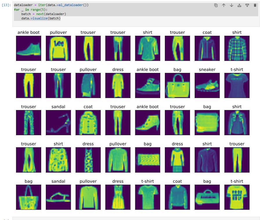
Tip. 위 iterator 중 첫 5개의 item을 출력 해 봤습니다.

dataloader = iter(data.val_dataloader())
for _ in range(5):
    batch = next(dataloader)
    data.visualize(batch)

참고로 전체를 디스플레이 하려면 아래와 같이 하면 됩니다.

dataloader = iter(data.val_dataloader())
for batch in dataloader:
    data.visualize(batch)

그런데 이렇게 하면 item들이 너무 많아서 다 display 하지는 못할 겁니다.

저 같은 경우는 50개만 출력 됐습니다.

위 메세지를 클릭하면 나머지 모두 다 출력 됩니다.

참고로 전체 아이템 갯수는 157개입니다.

dataloader = iter(data.val_dataloader())
num_items = len(dataloader)
print(num_items)

4.2.4. Summary

We now have a slightly more realistic dataset to use for classification. Fashion-MNIST is an apparel classification dataset consisting of images representing 10 categories. We will use this dataset in subsequent sections and chapters to evaluate various network designs, from a simple linear model to advanced residual networks. As we commonly do with images, we read them as a tensor of shape (batch size, number of channels, height, width). For now, we only have one channel as the images are grayscale (the visualization above use a false color palette for improved visibility).

이제 분류에 사용할 약간 더 현실적인 데이터 세트가 있습니다. Fashion-MNIST는 10개의 카테고리를 나타내는 이미지로 구성된 의류 분류 데이터셋입니다. 다음 섹션과 장에서 이 데이터 세트를 사용하여 간단한 선형 모델에서 고급 잔차 네트워크에 이르기까지 다양한 네트워크 디자인을 평가할 것입니다. 일반적으로 이미지와 마찬가지로 모양의 텐서(배치 크기, 채널 수, 높이, 너비)로 읽습니다. 지금은 이미지가 회색조이므로 채널이 하나만 있습니다(위의 시각화는 가시성을 높이기 위해 거짓 색상 팔레트를 사용함).

Lastly, data iterators are a key component for efficient performance. For instance, we might use GPUs for efficient image decompression, video transcoding, or other preprocessing. Whenever possible, you should rely on well-implemented data iterators that exploit high-performance computing to avoid slowing down your training loop.

마지막으로 데이터 반복자는 효율적인 성능을 위한 핵심 구성 요소입니다. 예를 들어 효율적인 이미지 압축 해제, 비디오 트랜스코딩 또는 기타 사전 처리를 위해 GPU를 사용할 수 있습니다. 가능할 때마다 고성능 컴퓨팅을 활용하는 잘 구현된 데이터 반복기에 의존하여 교육 루프 속도를 늦추지 않아야 합니다.

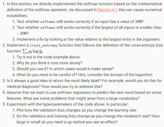
4.2.5. Exercises

1. Does reducing the batch_size (for instance, to 1) affect the reading performance?
2. The data iterator performance is important. Do you think the current implementation is fast enough? Explore various options to improve it. Use a system profiler to find out where the bottlenecks are.
3. Check out the framework’s online API documentation. Which other datasets are available?

https://d2l.ai/chapter_linear-classification/softmax-regression.html

4.1. Softmax Regression

In Section 3.1, we introduced linear regression, working through implementations from scratch in Section 3.4 and again using high-level APIs of a deep learning framework in Section 3.5 to do the heavy lifting.

섹션 3.1에서 우리는 선형 회귀를 소개했고, 섹션 3.4에서 처음부터 구현 작업을 수행하고 섹션 3.5에서 다시 딥 러닝 프레임워크의 고급 API를 사용하여 무거운 작업을 수행했습니다.

Regression is the hammer we reach for when we want to answer how much? or how many? questions. If you want to predict the number of dollars (price) at which a house will be sold, or the number of wins a baseball team might have, or the number of days that a patient will remain hospitalized before being discharged, then you are probably looking for a regression model. However, even within regression models, there are important distinctions. For instance, the price of a house will never be negative and changes might often be relative to its baseline price. As such, it might be more effective to regress on the logarithm of the price. Likewise, the number of days a patient spends in hospital is a discrete nonnegative random variable. As such, least mean squares might not be an ideal approach either. This sort of time-to-event modeling comes with a host of other complications that are dealt with in a specialized subfield called survival modeling.

회귀는 우리가 how much? 혹은 How many? 라는 질문에 대답하기 원할 때 사용할 수 있는 망치 입니다. 집이 팔릴 달러(가격), 야구팀의 승리 횟수 또는 환자가 퇴원하기 전에 입원할 일수를 예측하고 싶다면 아마도 Regression 모델을 찾을 것입니다. 그러나 회귀 모델 내에서도 중요한 차이점이 있습니다. 예를 들어, 주택 가격은 결코 음수가 되지 않으며 변경 사항은 종종 기준 가격에 상대적일 수 있습니다. 따라서 가격의 logarithm-로그-로 회귀하는 것이 더 효과적일 수 있습니다. 마찬가지로, 환자가 병원에서 보낸 일수는 discrete nonnegative random variable -음이 아닌 이산 랜덤 변수-입니다. 따라서 least mean squares -최소 평균 제곱-도 이상적인 접근 방식이 아닐 수 있습니다. 이러한 종류의 이벤트까지 걸리는 시간 모델링에는 survival modeling-생존 모델링-이라는 특수 하위 필드에서 처리되는 다른 복잡한 문제가 많이 있습니다.

The point here is not to overwhelm you but just to let you know that there is a lot more to estimation than simply minimizing squared errors. And more broadly, there’s a lot more to supervised learning than regression. In this section, we focus on classification problems where we put aside how much? questions and instead focus on which category? questions.

여기서 요점은 당신에게 기대감(뽕)을 주는 것이 아니라 단순히 squared error들을 minimize 하는 것보다 더 많은 estimation하는 방법이 있다는 것을 알려 드리기 위함입니다.  그리고 더 광범위하게 보면 supervised learning에는 regression보다 훨씬 더 많은 것이 있습니다. 이 섹션에서는 how much? 질문은 옆으로 치워 두고 classification problems에 촛점을 맞출 것입니다. 즉 어떤 category에 속하는가? 라는 질문에 초점을 맞출 것입니다. 

• Does this email belong in the spam folder or the inbox?
• 이 이메일이 스팸 폴더나 받은편지함에 속해 있습니까?
• Is this customer more likely to sign up or not to sign up for a subscription service?
• 이 고객이 구독 서비스에 가입할 가능성이 더 높습니까 아니면 가입하지 않을 가능성이 더 높습니까?
• Does this image depict a donkey, a dog, a cat, or a rooster?
• 이 이미지가 당나귀, 개, 고양이 또는 수탉 중 어느 종류를 묘사하고 있습니까?
• Which movie is Aston most likely to watch next?
• Aston이 다음에 볼 가능성이 가장 높은 영화는 무엇입니까?
• Which section of the book are you going to read next?
• 다음에 읽을 책의 섹션은 무엇입니까?

Colloquially, machine learning practitioners overload the word classification to describe two subtly different problems: (i) those where we are interested only in hard assignments of examples to categories (classes); and (ii) those where we wish to make soft assignments, i.e., to assess the probability that each category applies. The distinction tends to get blurred, in part, because often, even when we only care about hard assignments, we still use models that make soft assignments.

일반적으로 기계 학습 실무자는 두 가지 미묘하게 다른 문제를 설명하기 위해 분류라는 단어를 오버로드합니다. (i) 카테고리별 혹은 클래스별로 example들을 hard assignment하는 방법 그리고 (ii) soft assignment 하는 방법 이렇게 두가지가 있습니다. 예를 들어  각 범주가 적용될 probability -확률-을 assess -평가-하기 위한 경우를 들 수 있습니다. 한편으로 그 구분이 모호해지는 경향이 있는데, 그 이유는 hard assignments에만 신경을 쓰는 경우에도 여전히 soft assignments를 만드는 모델을 사용하기 때문입니다.

Even more, there are cases where more than one label might be true. For instance, a news article might simultaneously cover the topics of entertainment, business, and space flight, but not the topics of medicine or sports. Thus, categorizing it into one of the above categories on their own would not be very useful. This problem is commonly known as multi-label classification. See Tsoumakas and Katakis (2007) for an overview and Huang et al. (2015) for an effective algorithm when tagging images.

더군다나 둘 이상의 레이블이 참일 수 있는 경우가 있습니다. 예를 들어, 한 뉴스 기사는 엔터테인먼트, 비즈니스 및 우주 비행에 대한 주제를 동시에 다루지만 의학이나 스포츠에 대한 주제는 다루지 않을 수 있습니다. 따라서 위의 범주 중 하나로 분류하는 것은 그다지 유용하지 않습니다.   이 문제는 일반적으로 multi-label classification 다중 레이블 분류 로 알려져 있습니다.  전체 개요를 보려면 Tsoumakas and Katakis(2007) 그리고 이미지에 태그를 지정할 때 효과적인 알고리즘에 대한 내용을 보려면  Huang et al. (2015) 를 참조 하세요.

4.1.1. Classification

To get our feet wet, let’s start with a simple image classification problem. Here, each input consists of a 2×2 grayscale image. We can represent each pixel value with a single scalar, giving us four features x1, x2, x3, x4. Further, let’s assume that each image belongs to one among the categories “cat”, “chicken”, and “dog”.

이해를 돕기 위해 간단한 이미지 분류 문제부터 시작하겠습니다. 여기서 각 입력은 2×2 grayscale image로 구성됩니다. 단일 스칼라로 각 픽셀 값을 나타낼 수 있으므로 x1, x2, x3, x4의 네 가지 기능을 제공합니다. 또한 각 이미지가 "고양이", "닭", "개" 범주 중 하나에 속한다고 가정해 보겠습니다.

Next, we have to choose how to represent the labels. We have two obvious choices. Perhaps the most natural impulse would be to choose y ∈ {1,2,3}, where the integers represent {dog,cat,chicken} respectively. This is a great way of storing such information on a computer. If the categories had some natural ordering among them, say if we were trying to predict {baby,toddler,adolescent,young adult,adult,geriatric}, then it might even make sense to cast this as an ordinal regression problem and keep the labels in this format. See Moon et al. (2010) for an overview of different types of ranking loss functions and Beutel et al. (2014) for a Bayesian approach that addresses responses with more than one mode.

다음으로 레이블을 표시하는 방법을 선택해야 합니다. 우리에게는 두 가지 분명한 선택이 있습니다. 아마도 가장 자연스러운 충동은 y ∈ {1,2,3}을 선택하는 것일 것입니다. 여기서 정수는 각각 {dog,cat,chicken}을 나타냅니다. 이것은 그러한 정보를 컴퓨터에 저장하는 좋은 방법입니다. 카테고리에 자연스러운 순서가 있는 경우, 예를 들어 {아기,유아,청소년,청년,성인,노인}을 예측하려는 경우 이를 ordinal regression problem-서수 회귀 문제-로 캐스팅하고 레이블을 유지하는 것이 이치에 맞을 수도 있습니다.그리고 이 format으로 레이블들을 유지합니다.  다양한 유형의 ranking loss functions에 대한 내용은 See Moon et al. (2010)을 그리고   둘 이상의 모드로 응답을 처리하는 Bayesian approach에 대한 내용은 Beutel et al. (2014)를 참조 하세요.

In general, classification problems do not come with natural orderings among the classes. Fortunately, statisticians long ago invented a simple way to represent categorical data: the one-hot encoding. A one-hot encoding is a vector with as many components as we have categories. The component corresponding to a particular instance’s category is set to 1 and all other components are set to 0. In our case, a label y would be a three-dimensional vector, with (1,0,0) corresponding to “cat”, (0,1,0) to “chicken”, and (0,0,1) to “dog”:

일반적으로 분류 문제는 클래스 간의 자연스러운 순서와 함께 발생하지 않습니다. 다행스럽게도 통계학자들은 오래 전에 범주형 데이터를 나타내는 간단한 방법인 A one-hot encoding을 발명했습니다. A one-hot encoding은 우리가 가진 범주만큼 많은 구성 요소가 있는 벡터입니다. 특정 인스턴스의 범주에 해당하는 구성 요소는 1로 설정되고 다른 모든 구성 요소는 0으로 설정됩니다. 우리의 경우 레이블 y는 "cat"에 해당하는 (1,0,0)을 갖는 3차원 벡터입니다. (0,1,0)을 "닭"으로, (0,0,1)을 "개"로 설정 합니다.:

Python - sklearn.preprocessing.OneHotEncoder 예

import pandas as pd
from sklearn.preprocessing import OneHotEncoder

# create a sample dataframe with categorical data
df = pd.DataFrame({'animal': ['cat', 'chicken', 'dog', 'cat', 'dog']})

# create an instance of the OneHotEncoder class
encoder = OneHotEncoder()

# fit the encoder to the dataframe
encoder.fit(df)

# transform the dataframe using the encoder
transformed_df = encoder.transform(df).toarray()

# create a new dataframe with the transformed data
new_df = pd.DataFrame(transformed_df, columns=encoder.get_feature_names_out(['animal']))

# print the original and transformed dataframes
print('Original dataframe:\n', df)
print('Transformed dataframe:\n', new_df)

https://scikit-learn.org/stable/modules/generated/sklearn.preprocessing.OneHotEncoder.html

4.1.1.1. Linear Model

In order to estimate the conditional probabilities associated with all the possible classes, we need a model with multiple outputs, one per class. To address classification with linear models, we will need as many affine functions as we have outputs. Strictly speaking, we only need one fewer, since the last category has to be the difference between 1 and the sum of the other categories but for reasons of symmetry we use a slightly redundant parametrization. Each output corresponds to its own affine function. In our case, since we have 4 features and 3 possible output categories, we need 12 scalars to represent the weights (w with subscripts), and 3 scalars to represent the biases (b with subscripts). This yields:

가능한 모든 클래스와 관련된 조건부 확률을 추정하려면 클래스당 하나씩 여러 출력이 있는 모델이 필요합니다. (Open AI의 Embeddings 참조). 선형 모델로 분류를 처리하려면 출력 만큼  affine functions가 필요합니다. (어파인 변환(affine transformation)은 평행선과 거리 비율을 보존하는 기하학적 변환). 엄밀히 말하면 마지막 범주는 1과 다른 범주의 합 사이의 차이여야 하지만 대칭의 이유로 약간 중복된 매개변수화를 사용하기 때문에 하나만 더 적게 필요합니다. 각 출력은 자체 affine 함수에 해당합니다. 우리의 경우에는 4개의 features 와 3개의 가능한 출력 범주가 있으므로 가중치를 나타내는 데 12개의 스칼라(아래 첨자가 있는 w)와 편향을 나타내는 3개의 스칼라(아래 첨자가 있는 b)가 필요합니다. 결과는 다음과 같습니다.

Affine function 이란?

Affine function refers to a linear function that includes a constant offset. It is a mathematical function that transforms an input vector by performing a linear transformation and adding a constant vector. The term "affine" comes from the Latin word "affinis," which means "related" or "connected."

어파인 함수(Affine function)는 상수 오프셋을 포함하는 선형 함수를 의미합니다. 이는 입력 벡터에 선형 변환을 수행하고 상수 벡터를 더하여 입력 벡터를 변환하는 수학적인 함수입니다. "어파인"이라는 용어는 라틴어인 "affinis"에서 유래하며 "관련된" 또는 "연결된"을 의미합니다.

Mathematically, an affine function can be represented as: f(x) = Ax + b

수학적으로, 어파인 함수는 다음과 같이 표현될 수 있습니다: f(x) = Ax + b

Here, x is the input vector, A is a matrix representing the linear transformation, b is the constant offset vector, and f(x) is the output vector. The matrix A scales and rotates the input vector, while the offset vector b shifts the transformed vector.

여기서 x는 입력 벡터, A는 선형 변환을 나타내는 행렬, b는 상수 오프셋 벡터, f(x)는 출력 벡터입니다. 행렬 A는 입력 벡터를 스케일링하고 회전시키며, 오프셋 벡터 b는 변환된 벡터를 이동시킵니다.

The term "affine" is often used in contrast to "linear" functions. While linear functions preserve the origin (i.e., f(0) = 0), affine functions can have a non-zero constant offset. This offset allows affine functions to shift and translate the input space.

"어파인"이라는 용어는 종종 "선형" 함수와 대조적으로 사용됩니다. 선형 함수는 원점을 보존합니다(즉, f(0) = 0), 하지만 어파인 함수는 0이 아닌 상수 오프셋을 가질 수 있습니다. 이러한 오프셋은 어파인 함수가 입력 공간을 이동하고 변환할 수 있게 합니다.

Affine functions are commonly used in various areas of mathematics, including linear algebra, geometry, and optimization. In machine learning and deep learning, affine transformations are often used as building blocks for neural networks, where they contribute to modeling complex relationships between input features and the output.

어파인 함수는 선형 대수학, 기하학, 최적화 등 다양한 수학 분야에서 널리 사용됩니다. 머신러닝과 딥러닝에서는 어파인 변환은 종종 신경망의 구성 요소로 사용되며, 입력 특성과 출력 간의 복잡한 관계를 모델링하는 데 기여합니다.

In summary, an affine function is a linear function with a constant offset. It combines a linear transformation and a constant vector to map an input vector to an output vector. Affine functions are widely used in mathematics and serve as fundamental components in machine learning and deep learning models.

요약하면, 어파인 함수는 상수 오프셋을 포함하는 선형 함수입니다. 선형 변환과 상수 벡터의 결합을 통해 입력 벡터를 출력 벡터로 매핑합니다. 어파인 함수는 수학에서 널리 사용되며, 머신러닝과 딥러닝 모델에서 기본 구성 요소로 사용됩니다.

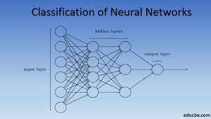
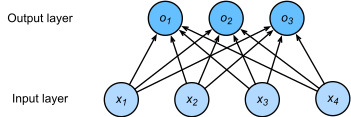
The corresponding neural network diagram is shown in Fig. 4.1.1. Just as in linear regression, we use a single-layer neural network. And since the calculation of each output, o1, o2, and o3, depends on all inputs, x1, x2, x3, and x4, the output layer can also be described as a fully connected layer.

해당 신경망 다이어그램은 그림 4.1.1에 나와 있습니다. 선형 회귀에서와 마찬가지로 단일 계층 신경망을 사용합니다. 그리고 각 출력 o1, o2, o3의 계산은 모든 입력 x1, x2, x3, x4에 따라 달라지므로 출력 레이어는 완전 연결 레이어라고도 할 수 있습니다.

For a more concise notation we use vectors and matrices: o=Wx+b (affine function) is much better suited for mathematics and code. Note that we have gathered all of our weights into a 3×4 matrix and all biases b∈R3 in a vector.

보다 간결한 표기법을 위해 벡터와 matrices-행렬-을 사용합니다. o=Wx+b는 수학과 코드에 훨씬 더 적합합니다. 모든 가중치를 3×4 행렬로 모았고 벡터의 모든 편향 b ∈ R3을 모았습니다.

4.1.1.2. The Softmax

Assuming a suitable loss function, we could try, directly, to minimize the difference between o and the labels y. While it turns out that treating classification as a vector-valued regression problem works surprisingly well, it is nonetheless lacking in the following ways:

적절한 loss function를 가정하면 o와 레이블 y 사이의 차이를 최소화하려고 직접 시도할 수 있습니다.classification 를 벡터 값 regression problem로 처리하는 것이 놀라울 정도로 잘 작동하는 것으로 밝혀졌지만 그럼에도 불구하고 다음과 같은 면에서 부족합니다.

• There is no guarantee that the outputs o_i sum up to 1 in the way we expect probabilities to behave.
• 확률이 동작할 것으로 기대하는 방식으로 출력 oi의 합이 1이 된다는 보장은 없습니다.
• There is no guarantee that the outputs o_i are even nonnegative, even if their outputs sum up to 1, or that they do not exceed 1.
• 출력의 합이 1이 되거나 1을 초과하지 않더라도 출력 oi가 음수가 아니라는 보장은 없습니다.

Both aspects render the estimation problem difficult to solve and the solution very brittle to outliers. For instance, if we assume that there is a positive linear dependency between the number of bedrooms and the likelihood that someone will buy a house, the probability might exceed 1 when it comes to buying a mansion! As such, we need a mechanism to “squish” the outputs.

두 측면 모두 estimation problem를 해결하기 어렵게 만들고 솔루션은 outliers (이상치, 예외치)에 매우 취약합니다. 예를 들어 침실 수와 누군가가 집을 살 likelihood  사이에 positive linear dependency이 있다고 가정하면 맨션을 살 때 확률은 1을 초과할 수 있습니다. As such, we need a mechanism to “squish” the outputs.
 

이 목표를 달성할 수 있는 방법에는 여러 가지가 있습니다. 예를 들어 출력 o가 y의 손상된 버전이라고 가정할 수 있습니다. 여기서 손상은 정규 분포에서 가져온 노이즈 E를 추가하여 발생합니다. 즉 다른 말로, y=o+E이며 Ei∼N(0,a2)입니다. 이것은 Fechner(1860)가 처음 소개한 소위  probit model입니다. 매력적이지만 softmax와 비교할 때 잘 작동하지 않으며 특히 좋은 최적화 문제로 이어지지 않습니다.

The probit model is a statistical model used for binary classification problems, where the goal is to predict the probability of an event occurring or not occurring. It is a type of generalized linear model (GLM) that assumes a linear relationship between the predictor variables and the cumulative distribution function (CDF) of a standard normal distribution.

프로빗 모델은 이진 분류 문제에 사용되는 통계 모델로, 어떤 사건이 발생할 확률 또는 발생하지 않을 확률을 예측하는 것이 목표입니다. 이는 일반화 선형 모델(Generalized Linear Model, GLM)의 한 유형으로, 예측 변수와 표준 정규 분포의 누적 분포 함수(Cumulative Distribution Function, CDF) 간에 선형 관계를 가정합니다.

In the probit model, the response variable is assumed to follow a binary distribution, typically a Bernoulli distribution. The model estimates the probability of the event based on a linear combination of predictor variables, transformed through the inverse of the standard normal cumulative distribution function, known as the probit function.

프로빗 모델에서는 반응 변수가 이항 분포(일반적으로 베르누이 분포)를 따른다고 가정합니다. 모델은 예측 변수의 선형 조합을 표준 정규 분포의 누적 분포 함수의 역함수인 프로빗 함수를 통해 변환하여 사건의 확률을 추정합니다.

The probit function is defined as the inverse of the cumulative distribution function (CDF) of a standard normal distribution. It maps the linear combination of predictors to a probability between 0 and 1. The probit model assumes that the linear combination of predictors, also known as the linear predictor, follows a normal distribution.

프로빗 함수는 표준 정규 분포의 누적 분포 함수(CDF)의 역함수로 정의됩니다. 이 함수는 예측 변수의 선형 조합을 0부터 1까지의 확률로 매핑합니다. 프로빗 모델은 선형 조합의 예측 변수(선형 예측기)가 정규 분포를 따른다고 가정합니다.

The estimation of the probit model is typically performed using maximum likelihood estimation (MLE). The MLE estimates the parameters of the model that maximize the likelihood of observing the given data. The likelihood function is derived from the assumed distribution of the response variable and the predicted probabilities.

프로빗 모델의 추정은 일반적으로 최대 우도 추정(Maximum Likelihood Estimation, MLE)을 사용하여 수행됩니다. MLE는 주어진 데이터를 관측할 가능성(우도)을 최대화하는 모델의 파라미터를 추정합니다. 우도 함수는 반응 변수의 가정된 분포와 예측된 확률에 기반하여 유도됩니다.

The probit model is often used when the relationship between the predictors and the response variable is expected to be nonlinear. It allows for flexible modeling of the relationship by capturing the nonlinearity through the inverse of the standard normal CDF. However, it assumes that the errors in the model are normally distributed.

프로빗 모델은 예측 변수와 반응 변수 간의 관계가 비선형일 것으로 예상될 때 자주 사용됩니다. 표준 정규 CDF의 역함수를 통해 비선형성을 포착하여 관계를 유연하게 모델링할 수 있습니다. 그러나 모델은 오차가 정규 분포를 따른다고 가정합니다.

In summary, the probit model is a statistical model used for binary classification tasks. It assumes a linear relationship between the predictor variables and the cumulative distribution function of a standard normal distribution. The model estimates the probability of an event using the probit function, and the parameters are estimated through maximum likelihood estimation.

Another way to accomplish this goal (and to ensure nonnegativity) is to use an exponential function P(y=i) ∝ exp ⁡oi. This does indeed satisfy the requirement that the conditional class probability increases with increasing oi, it is monotonic, and all probabilities are nonnegative. We can then transform these values so that they add up to 1 by dividing each by their sum. This process is called normalization. Putting these two pieces together gives us the softmax function:

요약하면, 프로빗 모델은 이진 분류 작업에 사용되는 통계 모델입니다. 예측 변수와 표준 정규 분포의 누적 분포 함수 간에 선형 관계를 가정합니다. 모델은 프로빗 함수를 사용하여 사건의 확률을 추정하며, 파라미터는 최대 우도 추정을 통해 추정됩니다.

목표를 달성하고 음수가 아님을 보장하는 또 다른 방법은 지수 함수 P(y=i) ∝ exp ⁡oi를 사용하는 것입니다. 이것은 실제로 조건부 클래스 확률이 oi가 증가함에 따라 증가하고 단조적이며 모든 확률이 음수가 아니라는 요구 사항을 충족합니다. 그런 다음 이 값을 변환하여 각 값을 합계로 나누어 합이 1이 되도록 할 수 있습니다. 이 프로세스를 normalization 정규화라고 합니다. 이 두 조각을 합치면 softmax 함수가 됩니다.

Note that the largest coordinate of o corresponds to the most likely class according to hat y. Moreover, because the softmax operation preserves the ordering among its arguments, we do not need to compute the softmax to determine which class has been assigned the highest probability.

o의 가장 큰 좌표는 hat y에 따라 가장 가능성이 높은 클래스에 해당합니다. 또한 softmax 작업은 인수 간의 순서를 유지하기 때문에 가장 높은 확률이 할당된 클래스를 결정하기 위해 softmax를 계산할 필요가 없습니다.

The idea of a softmax dates back to Gibbs, who adapted ideas from physics (Gibbs, 1902). Dating even further back, Boltzmann, the father of modern thermodynamics, used this trick to model a distribution over energy states in gas molecules. In particular, he discovered that the prevalence of a state of energy in a thermodynamic ensemble, such as the molecules in a gas, is proportional to exp⁡(−E/kT). Here, E is the energy of a state, T is the temperature, and k is the Boltzmann constant. When statisticians talk about increasing or decreasing the “temperature” of a statistical system, they refer to changing T in order to favor lower or higher energy states. Following Gibbs’ idea, energy equates to error. Energy-based models (Ranzato et al., 2007) use this point of view when describing problems in deep learning.

softmax 의 아이디어는 물리학의 아이디어를 채택한 Gibbs로 거슬러 올라갑니다(Gibbs, 1902). 훨씬 더 거슬러 올라가서, 현대 열역학의 아버지인 Boltzmann은 이 트릭을 사용하여 기체 분자의 에너지 상태에 대한 분포를 모델링했습니다. 특히 그는 기체 분자와 같은 열역학적 앙상블에서 에너지 상태의 보급이 exp⁡(-E/kT)에 비례한다는 사실을 발견했습니다. 여기서 E는 상태 에너지, T는 온도, k는 볼츠만 상수입니다. 통계학자가 통계 시스템의 "temperature 온도"를 높이거나 낮추는 것에 대해 이야기할 때 그들은 더 낮거나 더 높은 에너지 상태를 선호하기 위해 T를 변경하는 것을 말합니다. Gibbs의 아이디어에 따르면 에너지는 error 오류와 같습니다. 에너지 기반 모델(Ranzato et al., 2007)은 딥 러닝의 문제를 설명할 때 이 관점을 사용합니다.

What is softmax?

Softmax is a mathematical function that is often used in machine learning and deep learning for multiclass classification problems. It is a normalization function that takes a vector of real-valued numbers as input and outputs a vector of values between 0 and 1, where the values sum up to 1.

소프트맥스(Softmax)는 다중 클래스 분류 문제에서 자주 사용되는 수학적인 함수입니다. 이 함수는 실수값 벡터를 입력으로 받아 0과 1 사이의 값으로 구성된 벡터를 출력하며, 출력값들의 합은 1이 됩니다.

The softmax function is defined as follows for a vector z of length K: softmax(z_i) = exp(z_i) / (sum(exp(z_j)) for j=1 to K)

소프트맥스 함수는 길이가 K인 벡터 z에 대해 다음과 같이 정의됩니다:
소프트맥스(z_i) = exp(z_i) / (sum(exp(z_j)) for j=1 to K)

In simpler terms, the softmax function exponentiates each element of the input vector and divides it by the sum of the exponentiated values across all elements. This ensures that the output values represent probabilities or relative weights.

간단히 말하면, 소프트맥스 함수는 입력 벡터의 각 요소를 지수 함수로 변환한 후, 모든 요소의 exponentiated values -지수 함수 값-들의 합으로 각 값을 나눠줍니다. 이렇게 함으로써 출력값들은 확률이나 상대적인 가중치를 나타냅니다.

The softmax function is commonly used to convert a vector of real-valued scores or logits into a probability distribution over multiple classes. It assigns higher probabilities to larger values in the input vector, emphasizing the most confident predictions.

소프트맥스 함수는 vector of real-valued scores나 logits 를 multiple classes-다중 클래스-에 대한 probability distribution-확률 분포-로 변환하는 데에 자주 사용됩니다. 입력 벡터의 더 큰 값에 더 높은 확률을 할당하여  most confident predictions -가장 자신있는 예측-을  emphasizing -강조-합니다.

Softmax is particularly useful in multiclass classification tasks where each instance belongs to one of several mutually exclusive classes. By converting the scores into probabilities, softmax allows us to interpret the output as the likelihood or confidence of the input belonging to each class.

소프트맥스 함수는 각 인스턴스가 상호 배타적인 여러 클래스 중 하나에 속하는 다중 클래스 분류 작업에서 특히 유용합니다. 확률로 변환함으로써 출력을 각 클래스에 대한 확률이나 신뢰도로 해석할 수 있습니다.

During the training process, softmax is often used in conjunction with a loss function such as cross-entropy loss to measure the difference between the predicted probabilities and the true class labels. The goal is to minimize the loss and train the model to produce accurate and calibrated probability distributions.

훈련 과정에서는 소프트맥스 함수를 일반적으로 크로스 엔트로피 손실과 같은 손실 함수와 함께 사용하여 예측된 확률과 실제 클래스 레이블 사이의 차이를 측정합니다. 손실을 최소화하고 정확하고 균형 잡힌 확률 분포를 출력하도록 모델을 훈련하는 것이 목표입니다.

In summary, softmax is a normalization function used in multiclass classification to convert real-valued scores into probabilities. It is widely used in machine learning and deep learning for tasks such as image classification, natural language processing, and sentiment analysis.

요약하면, 소프트맥스는 실수값 스코어를 확률로 변환하는 정규화 함수로, 다중 클래스 분류에서 널리 사용됩니다. 이미지 분류, 자연어 처리, 감성 분석과 같은 머신러닝과 딥러닝 작업에서 널리 사용되는 함수입니다.

What is logits?

Logits refer to the vector of raw, unnormalized predictions generated by a model before applying a probability distribution function such as softmax. In other words, logits are the output of the last linear layer of a neural network before going through a non-linear activation function or probability normalization.

로짓(Logits)은 확률 분포 함수(softmax 등)를 적용하기 전 모델이 생성한 원시 및 정규화되지 않은 예측값 벡터를 의미합니다. 다른 말로하면, 로짓은 신경망의 마지막 선형 레이어의 출력으로, 비선형 활성화 함수나 확률 정규화를 거치기 전의 값입니다.

Logits can be thought of as the numerical values that represent the model's confidence or belief in each possible outcome or class. They are typically used in multi-class classification problems, where each class has its corresponding logit value. The relative magnitudes of the logits indicate the model's prediction probabilities for different classes.

로짓은 각 가능한 결과 또는 클래스에 대한 모델의 신뢰도나 확신을 나타내는 수치값으로 생각할 수 있습니다. 주로 다중 클래스 분류 문제에서 사용되며, 각 클래스에 해당하는 로짓 값이 존재합니다. 로짓의 상대적인 크기는 모델이 다른 클래스에 대해 예측한 확률을 나타냅니다.

Since logits are not normalized into probabilities, they can take any real value, positive or negative. Positive logits indicate a higher likelihood of the corresponding class, while negative logits suggest a lower likelihood. The actual probabilities are obtained by applying a softmax function to the logits, which normalizes the values and produces a valid probability distribution over the classes.

로짓은 확률로 정규화되지 않아 어떤 실수 값이든 가질 수 있습니다. 양수 로짓은 해당 클래스에 대한 예측 확률이 높음을 나타내며, 음수 로짓은 예측 확률이 낮음을 시사합니다. 실제 확률은 로짓에 softmax 함수를 적용하여 얻으며, 이 과정에서 값이 정규화되고 클래스에 대한 유효한 확률 분포가 생성됩니다.

Logits play a crucial role in determining the model's predictions and are often used in conjunction with a loss function during the training process. The model's parameters are optimized to minimize the loss by adjusting the logits to better align with the ground truth labels.

로짓은 모델의 예측을 결정하는 데 중요한 역할을 합니다. 훈련 과정에서 손실 함수와 함께 사용되며, 모델의 매개변수는 로짓을 조정하여 실제 레이블과 더 잘 일치하도록 최소화하는 방향으로 최적화됩니다.

In summary, logits are the unnormalized predictions generated by a model before converting them into probabilities. They represent the model's confidence or belief in different classes and are commonly used in multi-class classification tasks. The logits are then processed through a probability distribution function such as softmax to obtain valid probabilities for each class.

요약하면, 로짓은 확률로 변환되기 전에 모델이 생성한 정규화되지 않은 예측값을 의미합니다. 로짓은 모델이 다른 클래스에 대한 신뢰도나 확신을 나타내며, 주로 다중 클래스 분류 작업에서 사용됩니다. 로짓은 softmax와 같은 확률 분포 함수를 통해 정규화된 각 클래스의 확률을 얻기 위해 처리됩니다.

What does cross-entropy loss mean?

Cross-entropy loss, also known as log loss, is a commonly used loss function in machine learning and deep learning. It measures the dissimilarity between the predicted probability distribution and the true probability distribution of the target variables.

크로스 엔트로피 손실(Cross-entropy loss) 또는 로그 손실(Log loss)은 머신러닝과 딥러닝에서 일반적으로 사용되는 손실 함수입니다. 이는 예측된 확률 분포와 실제 타겟 변수의 확률 분포 간의 불일치를 측정합니다.

In classification tasks, where the goal is to assign an input to one of several possible classes, cross-entropy loss quantifies how well the predicted probabilities align with the true labels. It compares the predicted probabilities for each class with the actual binary indicators (0 or 1) of the true class.

분류 작업에서는 입력을 여러 가능한 클래스 중 하나에 할당하는 것이 목표입니다. 크로스 엔트로피 손실은 예측된 확률과 실제 레이블 간의 정확성을 평가합니다. 예측된 확률을 각 클래스의 실제 이진 지표(0 또는 1)와 비교합니다.

The formula for cross-entropy loss is as follows: L = -∑(y * log(p) + (1 - y) * log(1 - p))

크로스 엔트로피 손실의 수식은 다음과 같습니다: L = -∑(y * log(p) + (1 - y) * log(1 - p))

Here, y represents the true label (0 or 1) for the corresponding class, and p is the predicted probability for that class. The summation is taken over all classes. The term y * log(p) represents the contribution of the true class, while (1 - y) * log(1 - p) represents the contribution of the other classes.

여기서 y는 해당 클래스에 대한 실제 레이블(0 또는 1)을 나타내고, p는 해당 클래스에 대한 예측된 확률입니다. 합은 모든 클래스에 대해 계산됩니다. y * log(p)는 실제 클래스의 기여를 나타내고, (1 - y) * log(1 - p)는 다른 클래스의 기여를 나타냅니다.

Cross-entropy loss penalizes incorrect predictions heavily, assigning a higher loss when the predicted probability deviates from the true label. It encourages the model to learn accurate and confident predictions by minimizing the loss during the training process.

크로스 엔트로피 손실은 잘못된 예측에 대해 높은 페널티를 부여하여 예측된 확률이 실제 레이블과 얼마나 다른지를 평가합니다. 이를 통해 모델은 훈련 과정에서 손실을 최소화하여 정확하고 확신할 수 있는 예측을 학습하도록 장려됩니다.

The cross-entropy loss is commonly used in combination with softmax activation for multi-class classification tasks. The softmax function converts the logits into a probability distribution over the classes, and the cross-entropy loss measures the dissimilarity between the predicted probabilities and the true labels.

크로스 엔트로피 손실은 다중 클래스 분류 작업에서 주로 소프트맥스 활성화 함수와 함께 사용됩니다. 소프트맥스 함수는 로짓을 클래스별 확률 분포로 변환하고, 크로스 엔트로피 손실은 예측된 확률과 실제 레이블 간의 불일치를 측정합니다.

In summary, cross-entropy loss is a loss function that measures the dissimilarity between the predicted probability distribution and the true probability distribution. It is commonly used in classification tasks to train models by penalizing incorrect predictions and encouraging accurate and confident probability estimates.

요약하면, 크로스 엔트로피 손실은 예측된 확률 분포와 실제 확률 분포 간의 불일치를 측정하는 손실 함수입니다. 이는 분류 작업에서 잘못된 예측에 대해 페널티를 부여하고 정확하고 확신할 수 있는 확률 추정을 장려하기 위해 사용됩니다.

4.1.1.3. Vectorization

계산 효율성을 개선하기 위해 우리는 데이터의 미니배치에서 계산을 벡터화합니다. 차원(입력 수)이 d인 n개의 예제로 구성된 미니배치 X∈Rn×d가 주어졌다고 가정합니다. 또한 출력에 q 범주가 있다고 가정합니다. 그러면 가중치는 W∈Rd×q를 만족하고 바이어스는 b∈R1×q를 만족합니다.

This accelerates the dominant operation into a matrix-matrix product XW. Moreover, since each row in X represents a data example, the softmax operation itself can be computed rowwise: for each row of O, exponentiate all entries and then normalize them by the sum. Note, though, that care must be taken to avoid exponentiating and taking logarithms of large numbers, since this can cause numerical overflow or underflow. Deep learning frameworks take care of this automatically.

이것은 매트릭스-매트릭스 제품 XW로의 지배적인 작업을 가속화합니다. 또한 X의 각 행은 데이터 예를 나타내므로 softmax 작업 자체는 행 방향으로 계산할 수 있습니다. O의 각 행에 대해 모든 항목을 지수화한 다음 합계로 정규화합니다. 그러나 큰 수의 지수화 및 대수를 취하지 않도록 주의해야 합니다. 이렇게 하면 숫자 오버플로 또는 언더플로가 발생할 수 있기 때문입니다. 딥 러닝 프레임워크는 이를 자동으로 처리합니다.

4.1.2. Loss Function

Now that we have a mapping from features x to probabilities y^, we need a way to optimize the accuracy of this mapping. We will rely on maximum likelihood estimation, the very same concept that we encountered when providing a probabilistic justification for the mean squared error loss in Section 3.1.3.

이제 특성 x에서 확률 y^로의 매핑이 있으므로 이 매핑의 정확도를 최적화하는 방법이 필요합니다. 우리는 섹션 3.1.3에서 평균 제곱 오류 손실mean squared error loss에 대한 확률적 정당성probabilistic justification을 제공할 때 접했던 것과 동일한 개념인 최대 우도 추정 likelihood estimation에 의존할 것입니다.

maximum likelihood estimation

Maximum Likelihood Estimation (MLE) is a method used to estimate the parameters of a statistical model based on observed data. It is a widely used approach in statistical inference and machine learning. The goal of MLE is to find the set of parameter values that maximize the likelihood function, which measures how likely the observed data is under the given model.

최대 우도 추정(Maximum Likelihood Estimation, MLE)은 관측된 데이터를 기반으로 통계 모델의 파라미터를 추정하는 방법입니다. 이는 통계적 추론과 머신 러닝에서 널리 사용되는 접근 방법입니다. MLE의 목표는 우도 함수(Likelihood function)를 최대화하는 파라미터 값을 찾는 것으로, 이는 주어진 모델에서 관측된 데이터가 얼마나 가능한지를 측정합니다.

To understand MLE, let's consider a simple example. Suppose we have a dataset of independent and identically distributed (i.i.d.) observations, denoted as X1, X2, ..., Xn, where each observation is generated from a probability distribution with an unknown parameter θ. Our objective is to estimate the value of θ.

MLE를 이해하기 위해 간단한 예제를 살펴보겠습니다. 알려지지 않은 파라미터 θ를 가진 확률 분포에서 독립적이고 동일하게 분포된(i.i.d.) 관측 데이터셋 X1, X2, ..., Xn이 있다고 가정해봅시다. 우리의 목적은 θ의 값을 추정하는 것입니다.

The likelihood function, denoted as L(θ), measures the probability of observing the given data for a specific value of θ. In simple terms, it represents how likely the observed data is under the assumed model. The goal of MLE is to find the value of θ that maximizes the likelihood function, i.e., the value that makes the observed data most likely.

우도 함수 L(θ)는 특정 θ 값에 대해 주어진 데이터를 관측할 확률을 측정합니다. 간단히 말해, 가정된 모델 아래에서 관측된 데이터가 얼마나 가능한지를 나타냅니다. MLE의 목표는 우도 함수를 최대화하는 θ의 값을 찾는 것이며, 즉, 관측된 데이터를 가장 가능하게 만드는 값을 찾는 것입니다.

Mathematically, MLE can be formulated as follows: θ_hat = argmax(L(θ))

수학적으로 MLE는 다음과 같이 정의될 수 있습니다: θ_hat = argmax(L(θ))

To find the value of θ that maximizes the likelihood function, we differentiate the likelihood function with respect to θ and set it equal to zero. Solving this equation gives us the maximum likelihood estimate θ_hat.

우도 함수를 최대화하는 θ의 값을 찾기 위해, 우도 함수를 θ에 대해 미분하고 그 값을 0으로 설정합니다. 이 방정식을 풀면 최대 우도 추정값 θ_hat을 얻을 수 있습니다.

In practice, it is often more convenient to work with the log-likelihood function, denoted as log(L(θ)), because it simplifies calculations and does not affect the location of the maximum. Taking the logarithm of the likelihood function, we obtain the log-likelihood function. The maximum likelihood estimate can be obtained by maximizing the log-likelihood function instead.

실제로는 계산이 더 편리하고 최댓값에 영향을 주지 않는다는 이유로 로그-우도 함수(log-likelihood function)를 사용하는 것이 흔합니다. 로그-우도 함수는 우도 함수에 로그를 취한 함수입니다. 최대 우도 추정값은 로그-우도 함수를 최대화함으로써 얻을 수 있습니다.

MLE has several desirable properties, including consistency, asymptotic efficiency, and asymptotic normality under certain conditions. It is widely used in various statistical models, such as linear regression, logistic regression, and neural networks, to estimate the model parameters based on observed data.

MLE는 일정한 조건 하에서 일관성(consistency), 점근적 효율성(asymptotic efficiency), 점근적 정규성(asymptotic normality) 등 여러 가지 우수한 특성을 가지고 있습니다. 선형 회귀, 로지스틱 회귀, 신경망과 같은 다양한 통계 모델에서 관측된 데이터를 기반으로 모델 파라미터를 추정하는 데 널리 사용됩니다.

In summary, maximum likelihood estimation is a method used to estimate the parameters of a statistical model by finding the parameter values that maximize the likelihood function or the log-likelihood function. It provides a principled approach to parameter estimation based on observed data and is widely used in statistical inference and machine learning.

요약하면, 최대 우도 추정은 우도 함수 또는 로그-우도 함수를 최대화하는 파라미터 값을 찾아 통계 모델의 파라미터를 추정하는 방법입니다. 이는 관측된 데이터를 기반으로 한 파라미터 추정에 대한 원리적인 접근 방법을 제공하며, 통계적 추론과 머신 러닝에서 널리 사용됩니다.

4.1.2.1. Log-Likelihood

The softmax function gives us a vector y^, which we can interpret as (estimated) conditional probabilities of each class, given any input x, such as y^1 = P(y=cat∣x). In the following we assume that for a dataset with features X the labels Y are represented using a one-hot encoding label vector. We can compare the estimates with reality by checking how probable the actual classes are according to our model, given the features:

softmax 함수는 y^1 = P(y=cat∣x)와 같이 입력 x가 주어지면 각 클래스의 (추정된) 조건부 확률로 해석할 수 있는 벡터 y^를 제공합니다. 다음에서는 features  X가 있는 데이터 세트의 경우 레이블 Y가 one-hot encoding label vector를 사용하여 표현된다고 가정합니다. 주어진 특징에 따라 실제 클래스가 모델에 따라 얼마나 가능성이 있는지 확인하여 추정치를 현실과 비교할 수 있습니다.

We are allowed to use the factorization since we assume that each label is drawn independently from its respective distribution P(y∣x(i)). Since maximizing the product of terms is awkward, we take the negative logarithm to obtain the equivalent problem of minimizing the negative log-likelihood:

각 레이블이 해당 분포 P(y∣x(i))와 독립적으로 그려진다고 가정하기 때문에 분해를 사용할 수 있습니다. 항의 곱을 최대화하는 것은 어색하기 때문에 음의 로그 우도를 최소화하는 동등한 문제를 얻기 위해 음의 로그를 취합니다.

where for any pair of label y and model prediction y^ over q classes, the loss function l is

여기서 q 클래스에 대한 레이블 y 및 모델 예측 y^의 쌍에 대해 손실 함수 l은 다음과 같습니다.

For reasons explained later on, the loss function in (4.1.8) is commonly called the cross-entropy loss. Since y is a one-hot vector of length q, the sum over all its coordinates j vanishes for all but one term. Note that the loss l(y,y^) is bounded from below by 0 whenever y^ is a probability vector: no single entry is larger than 1, hence their negative logarithm cannot be lower than 0; l(y,y^)=0 only if we predict the actual label with certainty. This can never happen for any finite setting of the weights because taking a softmax output towards 1 requires taking the corresponding input oi to infinity (or all other outputs oj for j≠i to negative infinity). Even if our model could assign an output probability of 0, any error made when assigning such high confidence would incur infinite loss (−log⁡0=∞).

나중에 설명할 이유 때문에 (4.1.8)의 손실 함수는 일반적으로 cross-entropy loss 교차 엔트로피 손실이라고 합니다. y는 길이가 q인 원-핫 벡터이므로 모든 좌표 j에 대한 합은 하나를 제외한 모든 항에서 사라집니다. 손실 l(y,y^)은 y^가 확률 벡터일 때마다 아래에서 0으로 제한됩니다. 단일 항목이 1보다 크지 않으므로 음수 로그는 0보다 낮을 수 없습니다. l(y,y^)=0 실제 레이블을 확실하게 예측하는 경우에만. 1에 대한 소프트맥스 출력을 취하려면 해당 입력 oi를 무한대로(또는 j≠i에 대한 다른 모든 출력 oj를 음의 무한대로) 취해야 하기 때문에 가중치의 유한한 설정에서는 이런 일이 절대 발생할 수 없습니다. 모델이 0의 출력 확률을 할당할 수 있더라도 이러한 높은 신뢰도를 할당할 때 발생하는 모든 오류는 무한 손실(-log⁡0=∞)을 초래할 것입니다.

Log-Likelihood (Explained by ChatGPT)

The log-likelihood is a measure used to estimate the parameters of a probabilistic model. It is closely related to Maximum Likelihood Estimation (MLE) and is obtained by taking the logarithm of the likelihood function.

로그 우도(Log-Likelihood)는 확률 모델의 파라미터를 추정하는 데 사용되는 지표입니다. 최대 우도 추정(Maximum Likelihood Estimation, MLE)과 밀접한 관련이 있으며, 우도 함수(Likelihood function)에 로그를 적용하여 얻습니다.

The likelihood function represents the probability of the observed data given the parameters of the model. The log-likelihood is derived by taking the logarithm of the likelihood function, which simplifies calculations and facilitates differentiation for optimization purposes. Moreover, since the logarithm is a monotonic function, maximizing the log-likelihood is equivalent to maximizing the original likelihood function.

우도 함수는 모델의 파라미터에 대해 관측된 데이터가 발생할 확률을 나타냅니다. 로그 우도는 우도 함수에 로그를 취한 것으로, 계산을 단순화하고 최적화를 위한 미분을 용이하게 합니다. 또한 로그는 단조 증가 함수이므로 로그 우도를 최대화하는 것은 원래의 우도 함수를 최대화하는 것과 동일합니다.

Maximizing the log-likelihood is the same as the objective of MLE, which aims to find the parameter values that maximize the likelihood of the observed data. This estimation procedure helps determine the most suitable parameter values for the model. Numerical optimization algorithms can be employed to search for the parameter values that maximize the log-likelihood.

로그 우도를 최대화하는 것은 MLE의 목표와 동일하며, 관측된 데이터의 우도를 최대화하는 파라미터 값을 찾는 것입니다. 이 추정 과정을 통해 모델에 가장 적합한 파라미터 값을 결정할 수 있습니다. 로그 우도를 최대화하는 파라미터 값을 찾기 위해서는 수치적 최적화 알고리즘을 사용하여 로그 우도 함수를 최대화하는 파라미터 값을 탐색합니다.

The log-likelihood is commonly used in parameter estimation for probabilistic models. For example, in linear regression, the log-likelihood can be maximized to estimate the parameters by assuming an error term that follows a specific probability distribution.

로그 우도는 확률 모델의 파라미터 추정에서 흔히 사용됩니다. 예를 들어, 선형 회귀에서는 특정 확률 분포를 따르는 오차 항을 가정하여 로그 우도를 최대화함으로써 파라미터를 추정할 수 있습니다.

The log-likelihood is also useful for model comparison and evaluation. By comparing the log-likelihood values of different models, one can select the model with the highest likelihood. Additionally, the log-likelihood can be used to assess the predictive performance of a model.

로그 우도는 또한 모델 비교와 평가에 유용합니다. 서로 다른 모델들의 로그 우도 값을 비교하여 가장 높은 우도를 가진 모델을 선택할 수 있습니다. 또한 로그 우도를 사용하여 모델의 예측 성능을 평가할 수 있습니다.

In summary, the log-likelihood is a metric used in parameter estimation and model evaluation for probabilistic models. It is derived by taking the logarithm of the likelihood function and plays a crucial role in maximum likelihood estimation.

요약하면, 로그 우도는 확률 모델의 파라미터 추정과 모델 평가에 사용되는 지표로, 우도 함수에 로그를 적용하여 얻습니다. 최대 우도 추정에서 중요한 역할을 하며, 로그 우도를 최대화함으로써 가장 적합한 파라미터 값을 추정할 수 있습니다.

4.1.2.2. Softmax and Cross-Entropy Loss

Since the softmax function and the corresponding cross-entropy loss are so common, it is worth understanding a bit better how they are computed. Plugging (4.1.3) into the definition of the loss in (4.1.8) and using the definition of the softmax we obtain:

softmax 함수와 이에 상응하는 cross-entropy loss 교차 엔트로피 손실은 매우 일반적이므로 계산 방법을 좀 더 잘 이해할 가치가 있습니다. (4.1.3)을 (4.1.8)의 손실 정의에 연결하고 softmax의 정의를 사용하여 다음을 얻습니다.

To understand a bit better what is going on, consider the derivative with respect to any logit oj. We get

무슨 일이 일어나고 있는지 좀 더 잘 이해하려면 모든 로짓 oj에 대한 미분을 고려하십시오. 아래 내용을 얻을 수 있습니다.

In other words, the derivative is the difference between the probability assigned by our model, as expressed by the softmax operation, and what actually happened, as expressed by elements in the one-hot label vector. In this sense, it is very similar to what we saw in regression, where the gradient was the difference between the observation y and estimate y^. This is not coincidence. In any exponential family model, the gradients of the log-likelihood are given by precisely this term. This fact makes computing gradients easy in practice.

즉, 미분은 모델이 할당한 확률(softmax 연산으로 표현)과 실제로 발생한 것(원-핫 레이블 벡터의 요소로 표현) 간의 차이입니다. 이런 의미에서 기울기는 관측치 y와 추정치 y^의 차이인 회귀에서 본 것과 매우 유사합니다. 이것은 우연이 아닙니다. 모든 exponential family 모델에서 log-likelihood 로그 우도의 기울기는 정확히 이 용어로 제공됩니다. 이 사실은 실제로 그래디언트 계산을 쉽게 만듭니다.

Now consider the case where we observe not just a single outcome but an entire distribution over outcomes. We can use the same representation as before for the label y. The only difference is that rather than a vector containing only binary entries, say (0,0,1), we now have a generic probability vector, say (0.1,0.2,0.7). The math that we used previously to define the loss l in (4.1.8) still works out fine, just that the interpretation is slightly more general. It is the expected value of the loss for a distribution over labels. This loss is called the cross-entropy loss and it is one of the most commonly used losses for classification problems. We can demystify the name by introducing just the basics of information theory. In a nutshell, it measures the number of bits to encode what we see y relative to what we predict that should happen y^. We provide a very basic explanation in the following. For further details on information theory see Cover and Thomas (1999) or MacKay and Mac Kay (2003).

이제 단일 결과뿐만 아니라 결과에 대한 전체 분포를 관찰하는 경우를 고려하십시오. 레이블 y에 대해 이전과 동일한 표현을 사용할 수 있습니다. 유일한 차이점은 이진 항목만 포함하는 벡터(예: (0,0,1)) 대신 일반 확률 벡터(예: (0.1,0.2,0.7))가 있다는 것입니다. (4.1.8)에서 손실 l을 정의하기 위해 이전에 사용한 수학은 여전히 잘 작동하지만 해석이 약간 더 일반적입니다. 레이블에 대한 분포에 대한 손실의 예상 값입니다. 이 손실을 cross-entropy loss 교차 엔트로피 손실이라고 하며 분류 문제에서 가장 일반적으로 사용되는 손실 중 하나입니다. 우리는 정보 이론의 기초를 소개함으로써 그 이름을 이해할 수 있습니다. 간단히 말해서, 그것은 우리가 y^ 발생해야한다고 예측하는 것과 관련하여 우리가 보는 것을 인코딩하는 비트 수를 측정합니다. 다음에서 매우 기본적인 설명을 제공합니다. 정보 이론에 대한 자세한 내용은 Cover와 Thomas(1999) 또는 MacKay와 Mac Kay(2003)를 참조하십시오.

4.1.3. Information Theory Basics

Many deep learning papers use intuition and terms from information theory. To make sense of them, we need some common language. This is a survival guide. Information theory deals with the problem of encoding, decoding, transmitting, and manipulating information (also known as data).

많은 딥 러닝 논문은 정보 이론의 직관과 용어를 사용합니다. 그것들을 이해하려면 공통 언어가 필요합니다. 서바이벌 가이드입니다. Information theory 정보 이론은 정보(데이터라고도 함)를 인코딩, 디코딩, 전송 및 조작하는 문제를 다룹니다.

4.1.3.1. Entropy

The central idea in information theory is to quantify the amount of information contained in data. This places a limit on our ability to compress data. For a distribution P its entropy is defined as:

정보 이론의 핵심 아이디어는 데이터에 포함된 정보의 양을 정량화하는 것입니다. 이로 인해 데이터 압축 능력이 제한됩니다. 분포 P의 경우 엔트로피는 다음과 같이 정의됩니다.

One of the fundamental theorems of information theory states that in order to encode data drawn randomly from the distribution P, we need at least H[P] “nats” to encode it (Shannon, 1948). If you wonder what a “nat” is, it is the equivalent of bit but when using a code with base e rather than one with base 2. Thus, one nat is 1log⁡(2)≈1.44 bit.

정보 이론의 기본 정리 중 하나는 분포 P에서 무작위로 추출된 데이터를 인코딩하려면 적어도 H[P] "nats"가 인코딩되어야 한다는 것입니다(Shannon, 1948). "nat"이 무엇인지 궁금하다면, 그것은 비트와 동일하지만 밑이 2인 코드가 아닌 밑이 e인 코드를 사용할 때입니다. 따라서 하나의 nat는 1log⁡(2)≈1.44비트입니다.

4.1.3.2. Surprisal

You might be wondering what compression has to do with prediction. Imagine that we have a stream of data that we want to compress. If it is always easy for us to predict the next token, then this data is easy to compress. Take the extreme example where every token in the stream always takes the same value. That is a very boring data stream! And not only it is boring, but it is also easy to predict. Because they are always the same, we do not have to transmit any information to communicate the contents of the stream. Easy to predict, easy to compress.

압축이 예측과 어떤 관련이 있는지 궁금할 수 있습니다. 압축하려는 데이터 스트림이 있다고 상상해보십시오. 우리가 다음 토큰을 예측하는 것이 항상 쉽다면 이 데이터는 압축하기 쉽습니다. 스트림의 모든 토큰이 항상 동일한 값을 갖는 극단적인 예를 들어보십시오. 그것은 매우 지루한 데이터 스트림입니다! 지루할 뿐만 아니라 예측하기도 쉽습니다. 그것들은 항상 동일하기 때문에 스트림의 내용을 전달하기 위해 어떤 정보도 전송할 필요가 없습니다. 예측하기 쉽고 압축하기 쉽습니다.

However if we cannot perfectly predict every event, then we might sometimes be surprised. Our surprise is greater when we assigned an event lower probability. Claude Shannon settled on log⁡ 1/P(j)=−log⁡ P(j) to quantify one’s surprisal at observing an event j having assigned it a (subjective) probability P(j). The entropy defined in (4.1.11) is then the expected surprisal when one assigned the correct probabilities that truly match the data-generating process.

그러나 모든 사건을 완벽하게 예측할 수 없다면 때때로 놀랄 수도 있습니다. 이벤트에 더 낮은 확률을 할당했을 때 우리의 놀라움은 더 커졌습니다. Claude Shannon은 log⁡ 1/P(j)=−log⁡ P(j)로 정하여 (주관적) 확률 P(j)를 할당한 이벤트 j를 관찰했을 때의 놀라움을 정량화했습니다. (4.1.11)에 정의된 엔트로피는 데이터 생성 프로세스와 정확히 일치하는 올바른 확률을 할당했을 때 예상되는 놀라움입니다.

4.1.3.3. Cross-Entropy Revisited

So if entropy is the level of surprise experienced by someone who knows the true probability, then you might be wondering, what is cross-entropy? The cross-entropy from P to Q, denoted H(P,Q), is the expected surprisal of an observer with subjective probabilities Q upon seeing data that was actually generated according to probabilities P. This is given by H(P,Q)=def ∑j−P(j)log⁡Q(j). The lowest possible cross-entropy is achieved when P=Q. In this case, the cross-entropy from P to Q is H(P,P)=H(P).

따라서 엔트로피가 실제 확률을 아는 사람이 경험하는 놀라움의 수준이라면 교차 엔트로피가 무엇인지 궁금할 것입니다. H(P,Q)로 표시되는 P에서 Q까지의 교차 엔트로피는 확률 P에 따라 실제로 생성된 데이터를 보았을 때 주관적 확률 Q를 가진 관찰자의 예상되는 놀라움입니다. 이것은 H(P,Q)로 제공됩니다. =def ∑j-P(j)log⁡Q(j). 가능한 가장 낮은 교차 엔트로피는 P=Q일 때 달성됩니다. 이 경우 P에서 Q까지의 교차 엔트로피는 H(P,P)=H(P)입니다.

In short, we can think of the cross-entropy classification objective in two ways: (i) as maximizing the likelihood of the observed data; and (ii) as minimizing our surprisal (and thus the number of bits) required to communicate the labels.

요컨대 교차 엔트로피 분류 목표를 두 가지 방식으로 생각할 수 있습니다. (i) 관찰된 데이터의 우도를 최대화하는 것으로 (ii) 레이블을 전달하는 데 필요한 놀라움(따라서 비트 수)을 최소화합니다.

4.1.4. Summary and Discussion

In this section, we encountered the first nontrivial loss function, allowing us to optimize over discrete output spaces. Key in its design was that we took a probabilistic approach, treating discrete categories as instances of draws from a probability distribution. As a side effect, we encountered the softmax, a convenient activation function that transforms outputs of an ordinary neural network layer into valid discrete probability distributions. We saw that the derivative of the cross entropy loss when combined with softmax behaves very similarly to the derivative of squared error, namely by taking the difference between the expected behavior and its prediction. And, while we were only able to scratch the very surface of it, we encountered exciting connections to statistical physics and information theory.

이 섹션에서 우리는 이산 출력 공간을 최적화할 수 있는 첫 번째 중요한 손실 함수를 만났습니다. 디자인의 핵심은 우리가 확률적 접근 방식을 취하여 불연속 범주를 확률 분포에서 추출한 인스턴스로 취급한다는 것입니다. 부작용으로 일반 신경망 계층의 출력을 유효한 이산 확률 분포로 변환하는 편리한 활성화 함수인 softmax를 만났습니다. 우리는 softmax와 결합될 때 교차 엔트로피 손실의 파생물이 제곱 오차의 파생물과 매우 유사하게 동작한다는 것을 보았습니다. 그리고 우리는 표면적만 긁어모을 수 있었지만 통계 물리학 및 정보 이론과의 흥미로운 연관성을 발견했습니다.

While this is enough to get you on your way, and hopefully enough to whet your appetite, we hardly dived deep here. Among other things, we skipped over computational considerations. Specifically, for any fully connected layer with d inputs and q outputs, the parameterization and computational cost is O(dq), which can be prohibitively high in practice. Fortunately, this cost of transforming d inputs into q outputs can be reduced through approximation and compression. For instance Deep Fried Convnets (Yang et al., 2015) uses a combination of permutations, Fourier transforms, and scaling to reduce the cost from quadratic to log-linear. Similar techniques work for more advanced structural matrix approximations (Sindhwani et al., 2015). Lastly, we can use Quaternion-like decompositions to reduce the cost to O(dq/n), again if we are willing to trade off a small amount of accuracy for computational and storage cost (Zhang et al., 2021) based on a compression factor n. This is an active area of research. What makes it challenging is that we do not necessarily strive for the most compact representation or the smallest number of floating point operations but rather for the solution that can be executed most efficiently on modern GPUs.

이것은 당신에게 당신의 길을 안내하기에 충분하고 당신의 식욕을 돋우기에 충분하기를 바라지만 여기서는 거의 깊이 들어가지 않았습니다. 무엇보다도 우리는 계산상의 고려 사항을 건너뛰었습니다. 구체적으로 d 입력과 q 출력이 있는 완전히 연결된 레이어의 경우 매개변수화 및 계산 비용은 O(dq)이며 실제로는 엄청나게 높을 수 있습니다. 다행히 d 입력을 q 출력으로 변환하는 비용은 근사 및 압축을 통해 줄일 수 있습니다. 예를 들어 Deep Fried Convnets(Yang et al., 2015)는 순열, 푸리에 변환 및 스케일링의 조합을 사용하여 비용을 2차에서 로그 선형으로 줄입니다. 유사한 기술이 고급 구조 행렬 근사화에 사용됩니다(Sindhwani et al., 2015). 마지막으로 쿼터니언과 같은 분해를 사용하여 비용을 O(dq/n)으로 줄일 수 있습니다. 압축 계수 n. 이것은 활발한 연구 분야입니다. 이를 어렵게 만드는 것은 우리가 반드시 가장 컴팩트한 표현이나 가장 적은 수의 부동 소수점 연산을 위해 노력하는 것이 아니라 최신 GPU에서 가장 효율적으로 실행할 수 있는 솔루션을 위해 노력한다는 것입니다.

4.1.5. Exercises

https://d2l.ai/chapter_linear-classification/index.html

4. Linear Neural Networks for Classification

Now that you have worked through all of the mechanics you are ready to apply these skills to broader kinds of tasks. Even as we pivot towards classification, most of the plumbing remains the same: loading the data, passing it through the model, generating output, calculating the loss, taking gradients with respect to weights, and updating the model. However, the precise form of the targets, the parameterization of the output layer, and the choice of loss function will adapt to suit the classification setting.

이제 모든 메커니즘을 살펴보았으므로 이러한 기술을 더 광범위한 종류의 작업에 적용할 준비가 되었습니다. 분류로 전환하더라도 대부분의 배관 작업은 동일하게 유지됩니다. 즉, 데이터 로드, 모델에 데이터 전달, 출력 생성, 손실 계산, 가중치에 대한 그래디언트 적용 및 모델 업데이트입니다. 그러나 대상의 정확한 형태, 출력 계층의 매개변수화 및 손실 함수 선택은 분류 설정에 맞게 조정됩니다.

• 4.1. Softmax Regression
  • 4.1.1. Classification
  • 4.1.2. Loss Function
  • 4.1.3. Information Theory Basics
  • 4.1.4. Summary and Discussion
  • 4.1.5. Exercises
• 4.2. The Image Classification Dataset
  • 4.2.1. Loading the Dataset
  • 4.2.2. Reading a Minibatch
  • 4.2.3. Visualization
  • 4.2.4. Summary
  • 4.2.5. Exercises
• 4.3. The Base Classification Model
  • 4.3.1. The Classifier Class
  • 4.3.2. Accuracy
  • 4.3.3. Summary
  • 4.3.4. Exercises
• 4.4. Softmax Regression Implementation from Scratch
  • 4.4.1. The Softmax
  • 4.4.2. The Model
  • 4.4.3. The Cross-Entropy Loss
  • 4.4.4. Training
  • 4.4.5. Prediction
  • 4.4.6. Summary
  • 4.4.7. Exercises
• 4.5. Concise Implementation of Softmax Regression
  • 4.5.1. Defining the Model
  • 4.5.2. Softmax Revisited
  • 4.5.3. Training
  • 4.5.4. Summary
  • 4.5.5. Exercises
• 4.6. Generalization in Classification
  • 4.6.1. The Test Set
  • 4.6.2. Test Set Reuse
  • 4.6.3. Statistical Learning Theory
  • 4.6.4. Summary
  • 4.6.5. Exercises
• 4.7. Environment and Distribution Shift
  • 4.7.1. Types of Distribution Shift
  • 4.7.2. Examples of Distribution Shift
  • 4.7.3. Correction of Distribution Shift
  • 4.7.4. A Taxonomy of Learning Problems
  • 4.7.5. Fairness, Accountability, and Transparency in Machine Learning
  • 4.7.6. Summary
  • 4.7.7. Exercises

* Python and pip upgrade

python --version

pip install pip --upgrade

* D2L install

pip install d2l==1.0.0a0

* Pytorch install

pip install torch==1.12.0 torchvision==0.13.0

* Jupyter lab install

pip install jupyterlab

https://jupyterlab.readthedocs.io/en/latest/getting_started/installation.html

* Jupyter Lab 실행

python -m jupyterlab

==> Python 3 (ipykernel)

3.5. Concise Implementation of Linear Regression

Deep learning has witnessed a sort of Cambrian explosion over the past decade. The sheer number of techniques, applications and algorithms by far surpasses the progress of previous decades. This is due to a fortuitous combination of multiple factors, one of which is the powerful free tools offered by a number of open-source deep learning frameworks. Theano (Bergstra et al., 2010), DistBelief (Dean et al., 2012), and Caffe (Jia et al., 2014) arguably represent the first generation of such models that found widespread adoption. In contrast to earlier (seminal) works like SN2 (Simulateur Neuristique) (Bottou and Le Cun, 1988), which provided a Lisp-like programming experience, modern frameworks offer automatic differentiation and the convenience of Python. These frameworks allow us to automate and modularize the repetitive work of implementing gradient-based learning algorithms.

딥러닝은 지난 10년 동안 일종의 캄브리아기 폭발을 목격했습니다. 기술, 응용 프로그램 및 알고리즘의 수는 지난 수십 년 동안의 발전을 훨씬 능가합니다. 이는 여러 요소의 우연한 조합으로 인해 발생하며, 그 중 하나는 수많은 오픈 소스 딥 러닝 프레임워크에서 제공하는 강력한 무료 도구입니다. Theano(Bergstra et al., 2010), DistBelief(Dean et al., 2012) 및 Caffe(Jia et al., 2014)는 틀림없이 널리 채택된 이러한 모델의 1세대를 대표합니다. Lisp와 같은 프로그래밍 경험을 제공한 SN2(Simulateur Neuristique)(Bottou and Le Cun, 1988)와 같은 이전(세미널) 작업과 달리 현대 프레임워크는 자동 차별화와 Python의 편리함을 제공합니다. 이러한 프레임워크를 사용하면 경사 기반 학습 알고리즘을 구현하는 반복적인 작업을 자동화하고 모듈화할 수 있습니다.

In Section 3.4, we relied only on (i) tensors for data storage and linear algebra; and (ii) automatic differentiation for calculating gradients. In practice, because data iterators, loss functions, optimizers, and neural network layers are so common, modern libraries implement these components for us as well. In this section, we will show you how to implement the linear regression model from Section 3.4 concisely by using high-level APIs of deep learning frameworks.

섹션 3.4에서는 (i) 데이터 저장 및 선형 대수학을 위한 텐서; (ii) 기울기 계산을 위한 자동 미분. 실제로 데이터 반복기, 손실 함수, 최적화 프로그램 및 신경망 계층은 매우 일반적이기 때문에 최신 라이브러리에서는 이러한 구성 요소도 구현합니다. 이번 섹션에서는 딥러닝 프레임워크의 고급 API를 사용하여 3.4절의 선형 회귀 모델을 간결하게 구현하는 방법을 보여드리겠습니다.

import numpy as np
import torch
from torch import nn
from d2l import torch as d2l

3.5.1. Defining the Model

When we implemented linear regression from scratch in Section 3.4, we defined our model parameters explicitly and coded up the calculations to produce output using basic linear algebra operations. You should know how to do this. But once your models get more complex, and once you have to do this nearly every day, you will be glad of the assistance. The situation is similar to coding up your own blog from scratch. Doing it once or twice is rewarding and instructive, but you would be a lousy web developer if you spent a month reinventing the wheel.

섹션 3.4에서 선형 회귀를 처음부터 구현했을 때 모델 매개변수를 명시적으로 정의하고 계산을 코딩하여 기본 선형 대수 연산을 사용하여 출력을 생성했습니다. 이 작업을 수행하는 방법을 알아야 합니다. 그러나 모델이 더욱 복잡해지고 거의 매일 이 작업을 수행해야 한다면 도움을 받게 되어 기쁠 것입니다. 상황은 처음부터 자신의 블로그를 코딩하는 것과 유사합니다. 한두 번 하는 것은 보람 있고 유익하지만 한 달 동안 바퀴를 재발명하는 데 소비한다면 당신은 형편없는 웹 개발자가 될 것입니다.

For standard operations, we can use a framework’s predefined layers, which allow us to focus on the layers used to construct the model rather than worrying about their implementation. Recall the architecture of a single-layer network as described in Fig. 3.1.2. The layer is called fully connected, since each of its inputs is connected to each of its outputs by means of a matrix–vector multiplication.

표준 작업의 경우 프레임워크의 사전 정의된 레이어를 사용할 수 있습니다. 이를 통해 구현에 대해 걱정하는 대신 모델을 구성하는 데 사용되는 레이어에 집중할 수 있습니다. 그림 3.1.2에 설명된 단일 계층 네트워크의 아키텍처를 떠올려보세요. 각 입력이 행렬-벡터 곱셈을 통해 각 출력에 연결되므로 이 레이어를 완전 연결이라고 합니다.

In PyTorch, the fully connected layer is defined in Linear and LazyLinear classes (available since version 1.8.0). The latter allows users to specify merely the output dimension, while the former additionally asks for how many inputs go into this layer. Specifying input shapes is inconvenient and may require nontrivial calculations (such as in convolutional layers). Thus, for simplicity, we will use such “lazy” layers whenever we can.

PyTorch에서 완전 연결 계층은 Linear 및 LazyLinear 클래스(버전 1.8.0부터 사용 가능)에 정의됩니다. 후자를 사용하면 사용자가 출력 차원만 지정할 수 있는 반면, 전자는 이 레이어에 들어가는 입력 수를 추가로 묻습니다. 입력 모양을 지정하는 것은 불편하며 컨볼루셔널 레이어와 같은 중요한 계산이 필요할 수 있습니다. 따라서 단순화를 위해 가능할 때마다 이러한 "게으른" 레이어를 사용하겠습니다.

class LinearRegression(d2l.Module):  #@save
    """The linear regression model implemented with high-level APIs."""
    def __init__(self, lr):
        super().__init__()
        self.save_hyperparameters()
        self.net = nn.LazyLinear(1)
        self.net.weight.data.normal_(0, 0.01)
        self.net.bias.data.fill_(0)

In the forward method we just invoke the built-in __call__ method of the predefined layers to compute the outputs.

전달 방법에서는 미리 정의된 레이어의 내장 __call__ 방법을 호출하여 출력을 계산합니다.

@d2l.add_to_class(LinearRegression)  #@save
def forward(self, X):
    return self.net(X)

3.5.2. Defining the Loss Function

The MSELoss class computes the mean squared error (without the 1/2 factor in (3.1.5)). By default, MSELoss returns the average loss over examples. It is faster (and easier to use) than implementing our own.

MSELoss 클래스는 평균 제곱 오차를 계산합니다((3.1.5)의 요소 없이). 기본적으로 MSELoss는 예제에 대한 평균 손실을 반환합니다. 자체적으로 구현하는 것보다 더 빠르고 사용하기 쉽습니다.

@d2l.add_to_class(LinearRegression)  #@save
def loss(self, y_hat, y):
    fn = nn.MSELoss()
    return fn(y_hat, y)

3.5.3. Defining the Optimization Algorithm

Minibatch SGD is a standard tool for optimizing neural networks and thus PyTorch supports it alongside a number of variations on this algorithm in the optim module. When we instantiate an SGD instance, we specify the parameters to optimize over, obtainable from our model via self.parameters(), and the learning rate (self.lr) required by our optimization algorithm.

Minibatch SGD는 신경망 최적화를 위한 표준 도구이므로 PyTorch는 최적화 모듈에서 이 알고리즘의 다양한 변형과 함께 이를 지원합니다. SGD 인스턴스를 인스턴스화할 때 최적화할 매개변수(self.parameters()를 통해 모델에서 얻을 수 있음)와 최적화 알고리즘에 필요한 학습 속도(self.lr)를 지정합니다.

@d2l.add_to_class(LinearRegression)  #@save
def configure_optimizers(self):
    return torch.optim.SGD(self.parameters(), self.lr)

3.5.4. Training

You might have noticed that expressing our model through high-level APIs of a deep learning framework requires fewer lines of code. We did not have to allocate parameters individually, define our loss function, or implement minibatch SGD. Once we start working with much more complex models, the advantages of the high-level API will grow considerably.

딥 러닝 프레임워크의 고급 API를 통해 모델을 표현하는 데 더 적은 코드 줄이 필요하다는 점을 눈치채셨을 것입니다. 매개변수를 개별적으로 할당하거나, 손실 함수를 정의하거나, 미니배치 SGD를 구현할 필요가 없었습니다. 훨씬 더 복잡한 모델로 작업을 시작하면 고급 API의 장점이 상당히 커질 것입니다.

Now that we have all the basic pieces in place, the training loop itself is the same as the one we implemented from scratch. So we just call the fit method (introduced in Section 3.2.4), which relies on the implementation of the fit_epoch method in Section 3.4, to train our model.

이제 모든 기본 부분이 준비되었으므로 훈련 루프 자체는 처음부터 구현한 것과 동일합니다. 따라서 우리는 모델을 훈련시키기 위해 섹션 3.4의 fit_epoch 메소드 구현에 의존하는 fit 메소드(섹션 3.2.4에 소개됨)를 호출합니다.

model = LinearRegression(lr=0.03)
data = d2l.SyntheticRegressionData(w=torch.tensor([2, -3.4]), b=4.2)
trainer = d2l.Trainer(max_epochs=3)
trainer.fit(model, data)

Below, we compare the model parameters learned by training on finite data and the actual parameters that generated our dataset. To access parameters, we access the weights and bias of the layer that we need. As in our implementation from scratch, note that our estimated parameters are close to their true counterparts.

아래에서는 유한 데이터를 훈련하여 학습한 모델 매개변수와 데이터세트를 생성한 실제 매개변수를 비교합니다. 매개변수에 액세스하려면 필요한 레이어의 가중치와 편향에 액세스합니다. 처음부터 구현하는 것처럼 추정된 매개변수는 실제 매개변수와 가깝습니다.

@d2l.add_to_class(LinearRegression)  #@save
def get_w_b(self):
    return (self.net.weight.data, self.net.bias.data)
w, b = model.get_w_b()

print(f'error in estimating w: {data.w - w.reshape(data.w.shape)}')
print(f'error in estimating b: {data.b - b}')

error in estimating w: tensor([ 0.0094, -0.0030])
error in estimating b: tensor([0.0137])

3.5.5. Summary

This section contains the first implementation of a deep network (in this book) to tap into the conveniences afforded by modern deep learning frameworks, such as MXNet (Chen et al., 2015), JAX (Frostig et al., 2018), PyTorch (Paszke et al., 2019), and Tensorflow (Abadi et al., 2016). We used framework defaults for loading data, defining a layer, a loss function, an optimizer and a training loop. Whenever the framework provides all necessary features, it is generally a good idea to use them, since the library implementations of these components tend to be heavily optimized for performance and properly tested for reliability. At the same time, try not to forget that these modules can be implemented directly. This is especially important for aspiring researchers who wish to live on the leading edge of model development, where you will be inventing new components that cannot possibly exist in any current library.

이 섹션에는 MXNet(Chen et al., 2015), JAX(Frostig et al., 2018), PyTorch와 같은 최신 딥 러닝 프레임워크가 제공하는 편리함을 활용하기 위한 딥 네트워크(이 책)의 첫 번째 구현이 포함되어 있습니다. (Paszke 외, 2019) 및 Tensorflow(Abadi 외, 2016). 데이터 로드, 레이어 정의, 손실 함수, 최적화 프로그램 및 훈련 루프에 프레임워크 기본값을 사용했습니다. 프레임워크가 필요한 모든 기능을 제공할 때마다 일반적으로 이를 사용하는 것이 좋습니다. 이러한 구성 요소의 라이브러리 구현은 성능에 대해 크게 최적화되고 안정성에 대해 적절하게 테스트되는 경향이 있기 때문입니다. 동시에 이러한 모듈을 직접 구현할 수 있다는 점을 잊지 마십시오. 이는 현재 어떤 라이브러리에도 존재할 수 없는 새로운 구성 요소를 발명하게 될 모델 개발의 선두에 서기를 원하는 야심찬 연구자에게 특히 중요합니다.

In PyTorch, the data module provides tools for data processing, the nn module defines a large number of neural network layers and common loss functions. We can initialize the parameters by replacing their values with methods ending with _. Note that we need to specify the input dimensions of the network. While this is trivial for now, it can have significant knock-on effects when we want to design complex networks with many layers. Careful considerations of how to parametrize these networks is needed to allow portability.

PyTorch에서 데이터 모듈은 데이터 처리를 위한 도구를 제공하고, nn 모듈은 수많은 신경망 계층과 일반적인 손실 함수를 정의합니다. 매개변수 값을 _로 끝나는 메소드로 대체하여 매개변수를 초기화할 수 있습니다. 네트워크의 입력 차원을 지정해야 합니다. 지금은 이것이 사소한 일이지만, 많은 레이어로 구성된 복잡한 네트워크를 설계할 때 상당한 연쇄 효과를 가질 수 있습니다. 이식성을 허용하려면 이러한 네트워크를 매개변수화하는 방법에 대한 신중한 고려가 필요합니다.

3.5.6. Exercises

https://ko.d2l.ai/chapter_deep-learning-basics/fashion-mnist.html

D2L 모듈이 인스톨 되지 않아 소스 코드들을 실행 할 수 없음

https://d2l.ai/chapter_linear-regression/linear-regression-scratch.html

We are now ready to work through a fully functioning implementation of linear regression. In this section, we will implement the entire method from scratch, including (i) the model; (ii) the loss function; (iii) a minibatch stochastic gradient descent optimizer; and (iv) the training function that stitches all of these pieces together. Finally, we will run our synthetic data generator from Section 3.3 and apply our model on the resulting dataset. While modern deep learning frameworks can automate nearly all of this work, implementing things from scratch is the only way to make sure that you really know what you are doing. Moreover, when it is time to customize models, defining our own layers or loss functions, understanding how things work under the hood will prove handy. In this section, we will rely only on tensors and automatic differentiation. Later, we will introduce a more concise implementation, taking advantage of the bells and whistles of deep learning frameworks while retaining the structure of what follows below.

이제 우리는 선형 회귀의 완전한 기능 구현을 통해 작업할 준비가 되었습니다. 이 섹션에서는 (i) 모델; (ii) 손실 함수; (iii) 미니배치 확률적 경사하강법 최적화기; (iv) 이 모든 부분을 하나로 묶는 훈련 기능. 마지막으로 섹션 3.3의 합성 데이터 생성기를 실행하고 결과 데이터 세트에 모델을 적용합니다. 최신 딥 러닝 프레임워크는 이 작업을 거의 모두 자동화할 수 있지만, 처음부터 구현하는 것이 현재 수행 중인 작업이 무엇인지 확실히 알 수 있는 유일한 방법입니다. 더욱이, 모델을 맞춤화하고 자체 레이어나 손실 기능을 정의해야 할 때 내부적으로 작동하는 방식을 이해하는 것이 도움이 될 것입니다. 이 섹션에서는 텐서와 자동 미분에만 의존합니다. 나중에 우리는 아래의 구조를 유지하면서 딥 러닝 프레임워크의 부가 기능을 활용하는 보다 간결한 구현을 소개할 것입니다.

%matplotlib inline
import torch
from d2l import torch as d2l

3.4.1. Defining the Model

Before we can begin optimizing our model’s parameters by minibatch SGD, we need to have some parameters in the first place. In the following we initialize weights by drawing random numbers from a normal distribution with mean 0 and a standard deviation of 0.01. The magic number 0.01 often works well in practice, but you can specify a different value through the argument sigma. Moreover we set the bias to 0. Note that for object-oriented design we add the code to the __init__ method of a subclass of d2l.Module (introduced in Section 3.2.2).

미니배치 SGD로 모델 매개변수 최적화를 시작하려면 먼저 몇 가지 매개변수가 필요합니다. 다음에서는 평균이 0이고 표준편차가 0.01인 정규분포에서 난수를 뽑아 가중치를 초기화합니다. 매직 넘버 0.01은 실제로 잘 작동하는 경우가 많지만 시그마 인수를 통해 다른 값을 지정할 수 있습니다. 또한 바이어스를 0으로 설정했습니다. 객체 지향 설계의 경우 d2l.Module 하위 클래스의 __init__ 메서드에 코드를 추가합니다(섹션 3.2.2에 소개됨).

class LinearRegressionScratch(d2l.Module):  #@save
    """The linear regression model implemented from scratch."""
    def __init__(self, num_inputs, lr, sigma=0.01):
        super().__init__()
        self.save_hyperparameters()
        self.w = torch.normal(0, sigma, (num_inputs, 1), requires_grad=True)
        self.b = torch.zeros(1, requires_grad=True)

Next we must define our model, relating its input and parameters to its output. Using the same notation as (3.1.4) for our linear model we simply take the matrix–vector product of the input features X and the model weights w, and add the offset b to each example. The product Xw is a vector and b is a scalar. Because of the broadcasting mechanism (see Section 2.1.4), when we add a vector and a scalar, the scalar is added to each component of the vector. The resulting forward method is registered in the LinearRegressionScratch class via add_to_class (introduced in Section 3.2.1).

다음으로 입력과 매개변수를 출력과 연결하여 모델을 정의해야 합니다. 선형 모델에 대해 (3.1.4)와 동일한 표기법을 사용하여 입력 특성 X와 모델 가중치 w의 행렬-벡터 곱을 취하고 각 예에 오프셋 b를 추가합니다. 곱 Xw는 벡터이고 b는 스칼라입니다. 브로드캐스팅 메커니즘(섹션 2.1.4 참조)으로 인해 벡터와 스칼라를 추가하면 스칼라가 벡터의 각 구성 요소에 추가됩니다. 결과 전달 메서드는 add_to_class(섹션 3.2.1에 소개됨)를 통해 LinearRegressionScratch 클래스에 등록됩니다.

@d2l.add_to_class(LinearRegressionScratch)  #@save
def forward(self, X):
    return torch.matmul(X, self.w) + self.b

3.4.2. Defining the Loss Function

Since updating our model requires taking the gradient of our loss function, we ought to define the loss function first. Here we use the squared loss function in (3.1.5). In the implementation, we need to transform the true value y into the predicted value’s shape y_hat. The result returned by the following method will also have the same shape as y_hat. We also return the averaged loss value among all examples in the minibatch.

모델을 업데이트하려면 손실 함수의 기울기를 사용해야 하므로 손실 함수를 먼저 정의해야 합니다. 여기에서는 (3.1.5)의 제곱 손실 함수를 사용합니다. 구현에서는 실제 값 y를 예측 값의 모양 y_hat로 변환해야 합니다. 다음 메서드에서 반환된 결과도 y_hat과 동일한 모양을 갖습니다. 또한 미니배치의 모든 예제 중에서 평균 손실 값을 반환합니다.

3.4.3. Defining the Optimization Algorithm

As discussed in Section 3.1, linear regression has a closed-form solution. However, our goal here is to illustrate how to train more general neural networks, and that requires that we teach you how to use minibatch SGD. Hence we will take this opportunity to introduce your first working example of SGD. At each step, using a minibatch randomly drawn from our dataset, we estimate the gradient of the loss with respect to the parameters. Next, we update the parameters in the direction that may reduce the loss.

섹션 3.1에서 설명한 것처럼 선형 회귀에는 닫힌 형식의 솔루션이 있습니다. 그러나 여기서 우리의 목표는 보다 일반적인 신경망을 훈련하는 방법을 설명하는 것이며 이를 위해서는 미니배치 SGD를 사용하는 방법을 가르쳐야 합니다. 따라서 이번 기회에 SGD의 첫 번째 실제 사례를 소개하겠습니다. 각 단계에서 데이터세트에서 무작위로 추출된 미니배치를 사용하여 매개변수에 대한 손실 기울기를 추정합니다. 다음으로 손실을 줄일 수 있는 방향으로 매개변수를 업데이트합니다.

The following code applies the update, given a set of parameters, a learning rate lr. Since our loss is computed as an average over the minibatch, we do not need to adjust the learning rate against the batch size. In later chapters we will investigate how learning rates should be adjusted for very large minibatches as they arise in distributed large-scale learning. For now, we can ignore this dependency.

다음 코드는 학습률 lr이라는 매개변수 집합이 주어지면 업데이트를 적용합니다. 손실은 미니배치의 평균으로 계산되므로 배치 크기에 따라 학습률을 조정할 필요가 없습니다. 이후 장에서는 분산 대규모 학습에서 발생하는 매우 큰 미니 배치에 대해 학습 속도를 어떻게 조정해야 하는지 조사할 것입니다. 지금은 이 종속성을 무시해도 됩니다.

We define our SGD class, a subclass of d2l.HyperParameters (introduced in Section 3.2.1), to have a similar API as the built-in SGD optimizer. We update the parameters in the step method. The zero_grad method sets all gradients to 0, which must be run before a backpropagation step.

내장된 SGD 최적화 프로그램과 유사한 API를 갖도록 d2l.HyperParameters(섹션 3.2.1에서 소개)의 하위 클래스인 SGD 클래스를 정의합니다. step 메소드에서 매개변수를 업데이트합니다. zero_grad 메소드는 모든 그래디언트를 0으로 설정하며, 역전파 단계 전에 실행해야 합니다.

class SGD(d2l.HyperParameters):  #@save
    """Minibatch stochastic gradient descent."""
    def __init__(self, params, lr):
        self.save_hyperparameters()

    def step(self):
        for param in self.params:
            param -= self.lr * param.grad

    def zero_grad(self):
        for param in self.params:
            if param.grad is not None:
                param.grad.zero_()

We next define the configure_optimizers method, which returns an instance of the SGD class.

다음으로 SGD 클래스의 인스턴스를 반환하는configure_optimizers 메소드를 정의합니다.

@d2l.add_to_class(LinearRegressionScratch)  #@save
def configure_optimizers(self):
    return SGD([self.w, self.b], self.lr)

3.4.4. Training

Now that we have all of the parts in place (parameters, loss function, model, and optimizer), we are ready to implement the main training loop. It is crucial that you understand this code fully since you will employ similar training loops for every other deep learning model covered in this book. In each epoch, we iterate through the entire training dataset, passing once through every example (assuming that the number of examples is divisible by the batch size). In each iteration, we grab a minibatch of training examples, and compute its loss through the model’s training_step method. Then we compute the gradients with respect to each parameter. Finally, we will call the optimization algorithm to update the model parameters. In summary, we will execute the following loop:

이제 모든 부분(매개변수, 손실 함수, 모델 및 최적화 프로그램)이 준비되었으므로 기본 훈련 루프를 구현할 준비가 되었습니다. 이 책에서 다루는 다른 모든 딥러닝 모델에 대해 유사한 훈련 루프를 사용하게 되므로 이 코드를 완전히 이해하는 것이 중요합니다. 각 에포크에서 우리는 전체 교육 데이터 세트를 반복하여 모든 예시를 한 번 통과합니다(예제 수를 배치 크기로 나눌 수 있다고 가정). 각 반복에서 우리는 훈련 예제의 미니 배치를 잡고 모델의 training_step 방법을 통해 손실을 계산합니다. 그런 다음 각 매개변수에 대한 기울기를 계산합니다. 마지막으로 최적화 알고리즘을 호출하여 모델 매개변수를 업데이트합니다. 요약하면 다음 루프를 실행합니다.

Recall that the synthetic regression dataset that we generated in Section 3.3 does not provide a validation dataset. In most cases, however, we will want a validation dataset to measure our model quality. Here we pass the validation dataloader once in each epoch to measure the model performance. Following our object-oriented design, the prepare_batch and fit_epoch methods are registered in the d2l.Trainer class (introduced in Section 3.2.4).

섹션 3.3에서 생성한 합성 회귀 데이터세트는 검증 데이터세트를 제공하지 않는다는 점을 기억하세요. 그러나 대부분의 경우 모델 품질을 측정하기 위해 검증 데이터 세트가 필요합니다. 여기서는 모델 성능을 측정하기 위해 각 epoch마다 검증 데이터로더를 한 번씩 전달합니다. 객체 지향 설계에 따라 prepare_batch 및 fit_epoch 메소드는 d2l.Trainer 클래스에 등록됩니다(섹션 3.2.4에 소개됨).

@d2l.add_to_class(d2l.Trainer)  #@save
def prepare_batch(self, batch):
    return batch

@d2l.add_to_class(d2l.Trainer)  #@save
def fit_epoch(self):
    self.model.train()
    for batch in self.train_dataloader:
        loss = self.model.training_step(self.prepare_batch(batch))
        self.optim.zero_grad()
        with torch.no_grad():
            loss.backward()
            if self.gradient_clip_val > 0:  # To be discussed later
                self.clip_gradients(self.gradient_clip_val, self.model)
            self.optim.step()
        self.train_batch_idx += 1
    if self.val_dataloader is None:
        return
    self.model.eval()
    for batch in self.val_dataloader:
        with torch.no_grad():
            self.model.validation_step(self.prepare_batch(batch))
        self.val_batch_idx += 1

We are almost ready to train the model, but first we need some training data. Here we use the SyntheticRegressionData class and pass in some ground truth parameters. Then we train our model with the learning rate lr=0.03 and set max_epochs=3. Note that in general, both the number of epochs and the learning rate are hyperparameters. In general, setting hyperparameters is tricky and we will usually want to use a three-way split, one set for training, a second for hyperparameter selection, and the third reserved for the final evaluation. We elide these details for now but will revise them later.

모델을 훈련할 준비가 거의 완료되었지만 먼저 훈련 데이터가 필요합니다. 여기서는 SyntheticRegressionData 클래스를 사용하고 일부 실제 매개변수를 전달합니다. 그런 다음 학습률 lr=0.03으로 모델을 훈련하고 max_epochs=3으로 설정합니다. 일반적으로 에포크 수와 학습 속도는 모두 하이퍼파라미터입니다. 일반적으로 하이퍼파라미터를 설정하는 것은 까다로우며 일반적으로 3방향 분할을 사용하여 한 세트는 훈련용, 두 번째는 하이퍼파라미터 선택용, 세 번째는 최종 평가용으로 예약합니다. 지금은 이러한 세부 사항을 생략하고 나중에 수정하겠습니다.

model = LinearRegressionScratch(2, lr=0.03)
data = d2l.SyntheticRegressionData(w=torch.tensor([2, -3.4]), b=4.2)
trainer = d2l.Trainer(max_epochs=3)
trainer.fit(model, data)

Because we synthesized the dataset ourselves, we know precisely what the true parameters are. Thus, we can evaluate our success in training by comparing the true parameters with those that we learned through our training loop. Indeed they turn out to be very close to each other.

우리는 데이터세트를 직접 합성했기 때문에 실제 매개변수가 무엇인지 정확하게 알고 있습니다. 따라서 실제 매개변수와 훈련 루프를 통해 배운 매개변수를 비교하여 훈련 성공 여부를 평가할 수 있습니다. 실제로 그들은 서로 매우 가까운 것으로 밝혀졌습니다.

with torch.no_grad():
    print(f'error in estimating w: {data.w - model.w.reshape(data.w.shape)}')
    print(f'error in estimating b: {data.b - model.b}')

error in estimating w: tensor([ 0.1408, -0.1493])
error in estimating b: tensor([0.2130])

We should not take the ability to exactly recover the ground truth parameters for granted. In general, for deep models unique solutions for the parameters do not exist, and even for linear models, exactly recovering the parameters is only possible when no feature is linearly dependent on the others. However, in machine learning, we are often less concerned with recovering true underlying parameters, but rather with parameters that lead to highly accurate prediction (Vapnik, 1992). Fortunately, even on difficult optimization problems, stochastic gradient descent can often find remarkably good solutions, owing partly to the fact that, for deep networks, there exist many configurations of the parameters that lead to highly accurate prediction.

우리는 실측 매개변수를 정확하게 복구하는 능력을 당연하게 여겨서는 안 됩니다. 일반적으로 심층 모델의 경우 매개변수에 대한 고유한 솔루션이 존재하지 않으며 선형 모델의 경우에도 다른 기능에 선형적으로 종속되는 기능이 없는 경우에만 매개변수를 정확하게 복구하는 것이 가능합니다. 그러나 기계 학습에서 우리는 실제 기본 매개 변수를 복구하는 것보다 매우 정확한 예측으로 이어지는 매개 변수에 관심을 두는 경우가 많습니다(Vapnik, 1992). 다행스럽게도 어려운 최적화 문제에서도 확률적 경사하강법은 종종 매우 좋은 솔루션을 찾을 수 있는데, 이는 부분적으로 심층 네트워크의 경우 매우 정확한 예측으로 이어지는 매개변수의 많은 구성이 존재한다는 사실 때문입니다.

3.4.5. Summary

In this section, we took a significant step towards designing deep learning systems by implementing a fully functional neural network model and training loop. In this process, we built a data loader, a model, a loss function, an optimization procedure, and a visualization and monitoring tool. We did this by composing a Python object that contains all relevant components for training a model. While this is not yet a professional-grade implementation it is perfectly functional and code like this could already help you to solve small problems quickly. In the coming sections, we will see how to do this both more concisely (avoiding boilerplate code) and more efficiently (using our GPUs to their full potential).

이 섹션에서는 완전한 기능을 갖춘 신경망 모델과 훈련 루프를 구현하여 딥러닝 시스템을 설계하는 중요한 단계를 밟았습니다. 이 과정에서 우리는 데이터 로더, 모델, 손실 함수, 최적화 절차, 시각화 및 모니터링 도구를 구축했습니다. 우리는 모델 훈련을 위한 모든 관련 구성요소를 포함하는 Python 객체를 구성하여 이를 수행했습니다. 아직 전문가 수준의 구현은 아니지만 완벽하게 기능하며 이와 같은 코드는 이미 작은 문제를 신속하게 해결하는 데 도움이 될 수 있습니다. 다음 섹션에서는 이 작업을 보다 간결하게(보일러플레이트 코드 방지), 보다 효율적으로(GPU를 최대한 활용하는 방법) 수행하는 방법을 살펴보겠습니다.

3.4.6. Exercises

https://ko.d2l.ai/chapter_deep-learning-basics/softmax-regression.html

Linear Regression 이 아닌 Softmax Regression에 대한 개념 설명을 하는 장

https://d2l.ai/chapter_linear-regression/synthetic-regression-data.html

Machine learning is all about extracting information from data. So you might wonder, what could we possibly learn from synthetic data? While we might not care intrinsically about the patterns that we ourselves baked into an artificial data generating model, such datasets are nevertheless useful for didactic purposes, helping us to evaluate the properties of our learning algorithms and to confirm that our implementations work as expected. For example, if we create data for which the correct parameters are known a priori, then we can check that our model can in fact recover them.

머신러닝은 데이터에서 정보를 추출하는 것입니다. 그렇다면 합성 데이터에서 무엇을 배울 수 있을지 궁금할 것입니다. 우리는 인공 데이터 생성 모델에 직접 적용한 패턴에 본질적으로 관심을 두지 않을 수도 있지만 그럼에도 불구하고 이러한 데이터 세트는 교훈적인 목적으로 유용하며 학습 알고리즘의 속성을 평가하고 구현이 예상대로 작동하는지 확인하는 데 도움이 됩니다. 예를 들어, 올바른 매개변수가 선험적으로 알려진 데이터를 생성하는 경우 모델이 실제로 해당 매개변수를 복구할 수 있는지 확인할 수 있습니다.

%matplotlib inline
import random
import torch
from d2l import torch as d2l

3.3.1. Generating the Dataset

For this example, we will work in low dimension for succinctness. The following code snippet generates 1000 examples with 2-dimensional features drawn from a standard normal distribution. The resulting design matrix X belongs to ℝ **1000×2. We generate each label by applying a ground truth linear function, corrupting them via additive noise ϵ , drawn independently and identically for each example:

이 예에서는 간결성을 위해 낮은 차원에서 작업하겠습니다. 다음 코드 조각은 표준 정규 분포에서 추출된 2차원 특징을 사용하여 1000개의 예를 생성합니다. 결과 설계 행렬 X는 ℝ **1000×2에 속합니다. 우리는 Ground Truth 선형 함수를 적용하여 각 라벨을 생성하고, 각 예에 대해 독립적이고 동일하게 그려진 추가 노이즈 ϵ 를 통해 라벨을 손상시킵니다.

For convenience we assume that ϵ  is drawn from a normal distribution with mean μ =0 and standard deviation σ =0.01. Note that for object-oriented design we add the code to the __init__ method of a subclass of d2l.DataModule (introduced in Section 3.2.3). It is good practice to allow the setting of any additional hyperparameters. We accomplish this with save_hyperparameters(). The batch_size will be determined later.

편의상 ϵ는 평균 μ =0이고 표준편차 σ =0.01인 정규 분포에서 도출되었다고 가정합니다. 객체 지향 설계의 경우 d2l.DataModule 하위 클래스의 __init__ 메서드에 코드를 추가합니다(섹션 3.2.3에 소개됨). 추가 하이퍼파라미터 설정을 허용하는 것이 좋습니다. save_hyperparameters()를 사용하여 이를 수행합니다. Batch_size는 나중에 결정됩니다.

class SyntheticRegressionData(d2l.DataModule):  #@save
    """Synthetic data for linear regression."""
    def __init__(self, w, b, noise=0.01, num_train=1000, num_val=1000,
                 batch_size=32):
        super().__init__()
        self.save_hyperparameters()
        n = num_train + num_val
        self.X = torch.randn(n, len(w))
        noise = torch.randn(n, 1) * noise
        self.y = torch.matmul(self.X, w.reshape((-1, 1))) + b + noise

Below, we set the true parameters to w=[2,−3.4]⊤ and b=4.2. Later, we can check our estimated parameters against these ground truth values.

아래에서는 실제 매개변수를 w=[2,−3.4]⊤ 및 b=4.2로 설정했습니다. 나중에 이러한 실제 값과 비교하여 추정된 매개변수를 확인할 수 있습니다.

data = SyntheticRegressionData(w=torch.tensor([2, -3.4]), b=4.2)

Each row in features consists of a vector in ℝ**2 and each row in labels is a scalar. Let’s have a look at the first entry.

특성의 각 행은 ℝ**2의 벡터로 구성되고 레이블의 각 행은 스칼라입니다. 첫 번째 항목을 살펴보겠습니다.

print('features:', data.X[0],'\nlabel:', data.y[0])

features: tensor([0.9026, 1.0264])
label: tensor([2.5148])

3.3.2. Reading the Dataset

Training machine learning models often requires multiple passes over a dataset, grabbing one minibatch of examples at a time. This data is then used to update the model. To illustrate how this works, we implement the get_dataloader method, registering it in the SyntheticRegressionData class via add_to_class (introduced in Section 3.2.1). It takes a batch size, a matrix of features, and a vector of labels, and generates minibatches of size batch_size. As such, each minibatch consists of a tuple of features and labels. Note that we need to be mindful of whether we’re in training or validation mode: in the former, we will want to read the data in random order, whereas for the latter, being able to read data in a pre-defined order may be important for debugging purposes.

기계 학습 모델을 훈련하려면 한 번에 하나의 미니 배치 예제를 가져오는 데이터 세트에 대한 여러 번의 전달이 필요한 경우가 많습니다. 그런 다음 이 데이터는 모델을 업데이트하는 데 사용됩니다. 이것이 어떻게 작동하는지 설명하기 위해 get_dataloader 메소드를 구현하고 이를 add_to_class를 통해 SyntheticRegressionData 클래스에 등록합니다(섹션 3.2.1에 소개됨). 배치 크기, 기능 매트릭스, 레이블 벡터를 사용하고 배치_크기 크기의 미니 배치를 생성합니다. 따라서 각 미니 배치는 기능과 레이블의 튜플로 구성됩니다. 훈련 모드에 있는지 검증 모드에 있는지 주의해야 합니다. 전자에서는 데이터를 무작위 순서로 읽으려는 반면, 후자의 경우 미리 정의된 순서로 데이터를 읽을 수 있으면 디버깅 목적으로 중요합니다.

@d2l.add_to_class(SyntheticRegressionData)
def get_dataloader(self, train):
    if train:
        indices = list(range(0, self.num_train))
        # The examples are read in random order
        random.shuffle(indices)
    else:
        indices = list(range(self.num_train, self.num_train+self.num_val))
    for i in range(0, len(indices), self.batch_size):
        batch_indices = torch.tensor(indices[i: i+self.batch_size])
        yield self.X[batch_indices], self.y[batch_indices]

To build some intuition, let’s inspect the first minibatch of data. Each minibatch of features provides us with both its size and the dimensionality of input features. Likewise, our minibatch of labels will have a matching shape given by batch_size.

직관력을 키우기 위해 첫 번째 데이터 미니 배치를 살펴보겠습니다. 각 기능의 미니 배치는 입력 기능의 크기와 차원을 모두 제공합니다. 마찬가지로, 우리의 라벨 미니 배치는 배치_크기에 따라 일치하는 모양을 갖습니다.

X, y = next(iter(data.train_dataloader()))
print('X shape:', X.shape, '\ny shape:', y.shape)

X shape: torch.Size([32, 2])
y shape: torch.Size([32, 1])

While seemingly innocuous, the invocation of iter(data.train_dataloader()) illustrates the power of Python’s object-oriented design. Note that we added a method to the SyntheticRegressionData class after creating the data object. Nonetheless, the object benefits from the ex post facto addition of functionality to the class.

겉으로는 무해해 보이지만 iter(data.train_dataloader())의 호출은 Python의 객체 지향 설계의 힘을 보여줍니다. 데이터 객체를 생성한 후 SyntheticRegressionData 클래스에 메서드를 추가했습니다. 그럼에도 불구하고 객체는 사후에 클래스에 기능을 추가함으로써 이점을 얻습니다.

Throughout the iteration we obtain distinct minibatches until the entire dataset has been exhausted (try this). While the iteration implemented above is good for didactic purposes, it is inefficient in ways that might get us into trouble with real problems. For example, it requires that we load all the data in memory and that we perform lots of random memory access. The built-in iterators implemented in a deep learning framework are considerably more efficient and they can deal with sources such as data stored in files, data received via a stream, and data generated or processed on the fly. Next let’s try to implement the same method using built-in iterators.

반복을 통해 전체 데이터 세트가 소진될 때까지 별도의 미니 배치를 얻습니다(이것을 시도하십시오). 위에 구현된 반복은 교훈적인 목적으로는 좋지만 실제 문제를 해결할 수 있다는 점에서는 비효율적입니다. 예를 들어, 모든 데이터를 메모리에 로드하고 많은 무작위 메모리 액세스를 수행해야 합니다. 딥 러닝 프레임워크에 구현된 내장 반복자는 훨씬 더 효율적이며 파일에 저장된 데이터, 스트림을 통해 수신된 데이터, 즉석에서 생성되거나 처리되는 데이터와 같은 소스를 처리할 수 있습니다. 다음으로 내장된 반복자를 사용하여 동일한 메서드를 구현해 보겠습니다.

3.3.3. Concise Implementation of the Data Loade

Rather than writing our own iterator, we can call the existing API in a framework to load data. As before, we need a dataset with features X and labels y. Beyond that, we set batch_size in the built-in data loader and let it take care of shuffling examples efficiently.

자체 반복자를 작성하는 대신 프레임워크에서 기존 API를 호출하여 데이터를 로드할 수 있습니다. 이전과 마찬가지로 특성 X와 레이블 y가 있는 데이터 세트가 필요합니다. 그 외에도 내장 데이터 로더에서 배치_크기를 설정하고 셔플링 예제를 효율적으로 처리하도록 했습니다.

@d2l.add_to_class(d2l.DataModule)  #@save
def get_tensorloader(self, tensors, train, indices=slice(0, None)):
    tensors = tuple(a[indices] for a in tensors)
    dataset = torch.utils.data.TensorDataset(*tensors)
    return torch.utils.data.DataLoader(dataset, self.batch_size,
                                       shuffle=train)

@d2l.add_to_class(SyntheticRegressionData)  #@save
def get_dataloader(self, train):
    i = slice(0, self.num_train) if train else slice(self.num_train, None)
    return self.get_tensorloader((self.X, self.y), train, i)

The new data loader behaves just like the previous one, except that it is more efficient and has some added functionality.

새로운 데이터 로더는 더 효율적이고 몇 가지 추가 기능이 있다는 점을 제외하면 이전 데이터 로더와 동일하게 작동합니다.

X, y = next(iter(data.train_dataloader()))
print('X shape:', X.shape, '\ny shape:', y.shape)

X shape: torch.Size([32, 2])
y shape: torch.Size([32, 1])

For instance, the data loader provided by the framework API supports the built-in __len__ method, so we can query its length, i.e., the number of batches.

예를 들어 프레임워크 API에서 제공하는 데이터 로더는 내장된 __len__ 메서드를 지원하므로 해당 길이, 즉 배치 수를 쿼리할 수 있습니다.

len(data.train_dataloader())

32

3.3.4. Summary

https://ko.d2l.ai/chapter_deep-learning-basics/linear-regression-gluon.html

3.2. Object-Oriented Design for Implementation — Dive into Deep Learning 1.0.0-beta0 documentation (d2l.ai)

oo-design.ipynb - Colaboratory (google.com)

In our introduction to linear regression, we walked through various components including the data, the model, the loss function, and the optimization algorithm. Indeed, linear regression is one of the simplest machine learning models. Training it, however, uses many of the same components that other models in this book require. Therefore, before diving into the implementation details it is worth designing some of the APIs that we use throughout. Treating components in deep learning as objects, we can start by defining classes for these objects and their interactions. This object-oriented design for implementation will greatly streamline the presentation and you might even want to use it in your projects.

선형 회귀 소개에서는 데이터, 모델, 손실 함수 및 최적화 알고리즘을 포함한 다양한 구성 요소를 살펴보았습니다. 실제로 선형 회귀는 가장 간단한 기계 학습 모델 중 하나입니다. 그러나 이를 훈련하는 데는 이 책의 다른 모델에 필요한 것과 동일한 구성 요소가 많이 사용됩니다. 따라서 구현 세부 사항을 살펴보기 전에 우리가 전체적으로 사용하는 일부 API를 설계하는 것이 좋습니다. 딥 러닝의 구성 요소를 객체로 처리하려면 이러한 객체와 해당 상호 작용에 대한 클래스를 정의하는 것부터 시작할 수 있습니다. 구현을 위한 이 객체 지향 디자인은 프레젠테이션을 크게 간소화하며 프로젝트에서 이를 사용하고 싶을 수도 있습니다.

Inspired by open-source libraries such as PyTorch Lightning, at a high level we wish to have three classes: (i) Module contains models, losses, and optimization methods; (ii) DataModule provides data loaders for training and validation; (iii) both classes are combined using the Trainer class, which allows us to train models on a variety of hardware platforms. Most code in this book adapts Module and DataModule. We will touch upon the Trainer class only when we discuss GPUs, CPUs, parallel training, and optimization algorithms.

PyTorch Lightning과 같은 오픈 소스 라이브러리에서 영감을 받아 높은 수준에서 우리는 세 가지 클래스를 갖고 싶습니다. (i) 모듈에는 모델, 손실 및 최적화 방법이 포함되어 있습니다. (ii) DataModule은 교육 및 검증을 위한 데이터 로더를 제공합니다. (iii) 두 클래스 모두 Trainer 클래스를 사용하여 결합되어 다양한 하드웨어 플랫폼에서 모델을 교육할 수 있습니다. 이 책에 나오는 대부분의 코드는 Module과 DataModule을 채택합니다. GPU, CPU, 병렬 훈련 및 최적화 알고리즘을 논의할 때만 Trainer 클래스를 다룰 것입니다.

D2L 모듈 인스톨이 안 되서 실행 못함

import time
import numpy as np
import torch
from torch import nn
from d2l import torch as d2l

3.2.1. Utilities

We need a few utilities to simplify object-oriented programming in Jupyter notebooks. One of the challenges is that class definitions tend to be fairly long blocks of code. Notebook readability demands short code fragments, interspersed with explanations, a requirement incompatible with the style of programming common for Python libraries. The first utility function allows us to register functions as methods in a class after the class has been created. In fact, we can do so even after we have created instances of the class! It allows us to split the implementation of a class into multiple code blocks.

Jupyter 노트북에서 객체 지향 프로그래밍을 단순화하려면 몇 가지 유틸리티가 필요합니다. 과제 중 하나는 클래스 정의가 상당히 긴 코드 블록인 경향이 있다는 것입니다. 노트북 가독성을 위해서는 설명이 산재된 짧은 코드 조각이 필요합니다. 이는 Python 라이브러리에 일반적인 프로그래밍 스타일과 호환되지 않는 요구 사항입니다. 첫 번째 유틸리티 함수를 사용하면 클래스가 생성된 후 함수를 클래스의 메서드로 등록할 수 있습니다. 사실, 클래스의 인스턴스를 생성한 후에도 그렇게 할 수 있습니다! 이를 통해 클래스 구현을 여러 코드 블록으로 분할할 수 있습니다.

def add_to_class(Class):  #@save
    """Register functions as methods in created class."""
    def wrapper(obj):
        setattr(Class, obj.__name__, obj)
    return wrapper

Let’s have a quick look at how to use it. We plan to implement a class A with a method do. Instead of having code for both A and do in the same code block, we can first declare the class A and create an instance a.

사용법을 간단히 살펴보겠습니다. 우리는 do 메소드를 사용하여 클래스 A를 구현할 계획입니다. A와 do에 대한 코드를 동일한 코드 블록에 두는 대신 먼저 클래스 A를 선언하고 인스턴스 a를 만들 수 있습니다.

class A:
    def __init__(self):
        self.b = 1

a = A()

Next we define the method do as we normally would, but not in class A’s scope. Instead, we decorate this method by add_to_class with class A as its argument. In doing so, the method is able to access the member variables of A just as we would expect had it been included as part of A’s definition. Let’s see what happens when we invoke it for the instance a.

다음으로 우리는 평소처럼 do 메서드를 정의하지만 클래스 A의 범위에서는 그렇지 않습니다. 대신, 클래스 A를 인수로 사용하여 add_to_class로 이 메소드를 장식합니다. 그렇게 함으로써, 메소드는 A의 정의의 일부로 포함되었을 때 예상했던 것처럼 A의 멤버 변수에 액세스할 수 있습니다. 인스턴스 a에 대해 호출하면 어떤 일이 발생하는지 살펴보겠습니다.

@add_to_class(A)
def do(self):
    print('Class attribute "b" is', self.b)

a.do()

The second one is a utility class that saves all arguments in a class’s __init__ method as class attributes. This allows us to extend constructor call signatures implicitly without additional code.

두 번째는 클래스 속성으로 클래스의 __init__ 메서드에 있는 모든 인수를 저장하는 유틸리티 클래스입니다. 이를 통해 추가 코드 없이 생성자 호출 서명을 암시적으로 확장할 수 있습니다.

class HyperParameters:  #@save
    """The base class of hyperparameters."""
    def save_hyperparameters(self, ignore=[]):
        raise NotImplemented

We defer its implementation into Section 23.7. To use it, we define our class that inherits from HyperParameters and calls save_hyperparameters in the __init__ method.

우리는 그 구현을 섹션 23.7로 연기합니다. 이를 사용하려면 HyperParameters에서 상속하고 __init__ 메서드에서 save_hyperparameters를 호출하는 클래스를 정의합니다.

# Call the fully implemented HyperParameters class saved in d2l
class B(d2l.HyperParameters):
    def __init__(self, a, b, c):
        self.save_hyperparameters(ignore=['c'])
        print('self.a =', self.a, 'self.b =', self.b)
        print('There is no self.c =', not hasattr(self, 'c'))

b = B(a=1, b=2, c=3)

self.a = 1 self.b = 2
There is no self.c = True

The final utility allows us to plot experiment progress interactively while it is going on. In deference to the much more powerful (and complex) TensorBoard we name it ProgressBoard. The implementation is deferred to Section 23.7. For now, let’s simply see it in action.

최종 유틸리티를 사용하면 실험이 진행되는 동안 대화식으로 실험 진행 상황을 플롯할 수 있습니다. 훨씬 더 강력하고 복잡한 TensorBoard를 존중하여 우리는 이를 ProgressBoard라고 명명합니다. 구현은 섹션 23.7로 연기됩니다. 지금은 실제로 작동하는 모습을 살펴보겠습니다.

The draw method plots a point (x, y) in the figure, with label specified in the legend. The optional every_n smooths the line by only showing 1/n points in the figure. Their values are averaged from the n neighbor points in the original figure.

draw 메소드는 범례에 지정된 레이블을 사용하여 그림의 점(x, y)을 플롯합니다. 선택적 Every_n은 그림에 1/n 지점만 표시하여 선을 매끄럽게 만듭니다. 해당 값은 원래 그림의 n개 이웃 점에서 평균을 냅니다.

class ProgressBoard(d2l.HyperParameters):  #@save
    """The board that plots data points in animation."""
    def __init__(self, xlabel=None, ylabel=None, xlim=None,
                 ylim=None, xscale='linear', yscale='linear',
                 ls=['-', '--', '-.', ':'], colors=['C0', 'C1', 'C2', 'C3'],
                 fig=None, axes=None, figsize=(3.5, 2.5), display=True):
        self.save_hyperparameters()

    def draw(self, x, y, label, every_n=1):
        raise NotImplemented

In the following example, we draw sin and cos with a different smoothness. If you run this code block, you will see the lines grow in animation.

다음 예에서는 다른 부드러움으로 sin과 cos를 그립니다. 이 코드 블록을 실행하면 애니메이션에서 줄이 늘어나는 것을 볼 수 있습니다.

board = d2l.ProgressBoard('x')
for x in np.arange(0, 10, 0.1):
    board.draw(x, np.sin(x), 'sin', every_n=2)
    board.draw(x, np.cos(x), 'cos', every_n=10)

3.2.2. Models

The Module class is the base class of all models we will implement. At the very least we need three methods. The first, __init__, stores the learnable parameters, the training_step method accepts a data batch to return the loss value, and finally, configure_optimizers returns the optimization method, or a list of them, that is used to update the learnable parameters. Optionally we can define validation_step to report the evaluation measures. Sometimes we put the code for computing the output into a separate forward method to make it more reusable.

모듈 클래스는 우리가 구현할 모든 모델의 기본 클래스입니다. 최소한 세 가지 방법이 필요합니다. 첫 번째 __init__는 학습 가능한 매개변수를 저장하고, training_step 메서드는 데이터 배치를 받아 손실 값을 반환하며, 마지막으로configure_optimizers는 학습 가능한 매개변수를 업데이트하는 데 사용되는 최적화 메서드 또는 그 목록을 반환합니다. 선택적으로 평가 측정값을 보고하기 위해 유효성 검사 단계를 정의할 수 있습니다. 때때로 우리는 출력을 더 쉽게 재사용할 수 있도록 별도의 전달 메서드에 출력을 계산하는 코드를 넣습니다.

class Module(nn.Module, d2l.HyperParameters):  #@save
    """The base class of models."""
    def __init__(self, plot_train_per_epoch=2, plot_valid_per_epoch=1):
        super().__init__()
        self.save_hyperparameters()
        self.board = ProgressBoard()

    def loss(self, y_hat, y):
        raise NotImplementedError

    def forward(self, X):
        assert hasattr(self, 'net'), 'Neural network is defined'
        return self.net(X)

    def plot(self, key, value, train):
        """Plot a point in animation."""
        assert hasattr(self, 'trainer'), 'Trainer is not inited'
        self.board.xlabel = 'epoch'
        if train:
            x = self.trainer.train_batch_idx / \
                self.trainer.num_train_batches
            n = self.trainer.num_train_batches / \
                self.plot_train_per_epoch
        else:
            x = self.trainer.epoch + 1
            n = self.trainer.num_val_batches / \
                self.plot_valid_per_epoch
        self.board.draw(x, value.to(d2l.cpu()).detach().numpy(),
                        ('train_' if train else 'val_') + key,
                        every_n=int(n))

    def training_step(self, batch):
        l = self.loss(self(*batch[:-1]), batch[-1])
        self.plot('loss', l, train=True)
        return l

    def validation_step(self, batch):
        l = self.loss(self(*batch[:-1]), batch[-1])
        self.plot('loss', l, train=False)

    def configure_optimizers(self):
        raise NotImplementedError

You may notice that Module is a subclass of nn.Module, the base class of neural networks in PyTorch. It provides convenient features for handling neural networks. For example, if we define a forward method, such as forward(self, X), then for an instance a we can invoke this method by a(X). This works since it calls the forward method in the built-in __call__ method. You can find more details and examples about nn.Module in Section 6.1.

Module은 PyTorch 신경망의 기본 클래스인 nn.Module의 하위 클래스라는 것을 알 수 있습니다. 신경망 처리에 편리한 기능을 제공합니다. 예를 들어, 전달(self, X)와 같은 전달 메서드를 정의하면 인스턴스 a에 대해 이 메서드를 a(X)로 호출할 수 있습니다. 이는 내장된 __call__ 메서드에서 전달 메서드를 호출하기 때문에 작동합니다. 섹션 6.1에서 nn.Module에 대한 자세한 내용과 예제를 확인할 수 있습니다.

3.2.3. Data

The DataModule class is the base class for data. Quite frequently the __init__ method is used to prepare the data. This includes downloading and preprocessing if needed. The train_dataloader returns the data loader for the training dataset. A data loader is a (Python) generator that yields a data batch each time it is used. This batch is then fed into the training_step method of Module to compute the loss. There is an optional val_dataloader to return the validation dataset loader. It behaves in the same manner, except that it yields data batches for the validation_step method in Module.

DataModule 클래스는 데이터의 기본 클래스입니다. 데이터를 준비하는 데 __init__ 메서드가 자주 사용됩니다. 여기에는 필요한 경우 다운로드 및 전처리가 포함됩니다. train_dataloader는 훈련 데이터 세트에 대한 데이터 로더를 반환합니다. 데이터 로더는 사용될 때마다 데이터 배치를 생성하는 (Python) 생성기입니다. 그런 다음 이 배치는 모듈의 training_step 메서드에 입력되어 손실을 계산합니다. 유효성 검사 데이터 세트 로더를 반환하는 선택적 val_dataloader가 있습니다. Module의 유효성 검사 단계 메서드에 대한 데이터 배치를 생성한다는 점을 제외하면 동일한 방식으로 작동합니다.

class DataModule(d2l.HyperParameters):  #@save
    """The base class of data."""
    def __init__(self, root='../data', num_workers=4):
        self.save_hyperparameters()

    def get_dataloader(self, train):
        raise NotImplementedError

    def train_dataloader(self):
        return self.get_dataloader(train=True)

    def val_dataloader(self):
        return self.get_dataloader(train=False)

3.2.4. Training

The Trainer class trains the learnable parameters in the Module class with data specified in DataModule. The key method is fit, which accepts two arguments: model, an instance of Module, and data, an instance of DataModule. It then iterates over the entire dataset max_epochs times to train the model. As before, we will defer the implementation of this method to later chapters.

Trainer 클래스는 DataModule에 지정된 데이터를 사용하여 Module 클래스의 학습 가능한 매개변수를 교육합니다. 핵심 메소드는 fit입니다. 이는 Module의 인스턴스인 model과 DataModule의 인스턴스인 data라는 두 가지 인수를 허용합니다. 그런 다음 전체 데이터 세트 max_epochs 회를 반복하여 모델을 교육합니다. 이전과 마찬가지로 이 메서드의 구현은 이후 장으로 미루겠습니다.

class Trainer(d2l.HyperParameters):  #@save
    """The base class for training models with data."""
    def __init__(self, max_epochs, num_gpus=0, gradient_clip_val=0):
        self.save_hyperparameters()
        assert num_gpus == 0, 'No GPU support yet'

    def prepare_data(self, data):
        self.train_dataloader = data.train_dataloader()
        self.val_dataloader = data.val_dataloader()
        self.num_train_batches = len(self.train_dataloader)
        self.num_val_batches = (len(self.val_dataloader)
                                if self.val_dataloader is not None else 0)

    def prepare_model(self, model):
        model.trainer = self
        model.board.xlim = [0, self.max_epochs]
        self.model = model

    def fit(self, model, data):
        self.prepare_data(data)
        self.prepare_model(model)
        self.optim = model.configure_optimizers()
        self.epoch = 0
        self.train_batch_idx = 0
        self.val_batch_idx = 0
        for self.epoch in range(self.max_epochs):
            self.fit_epoch()

    def fit_epoch(self):
        raise NotImplementedError