

https://d2l.ai/chapter_linear-regression/generalization.html
3.6. Generalization — Dive into Deep Learning 1.0.3 documentation
d2l.ai
3.6. Generalization
Consider two college students diligently preparing for their final exam. Commonly, this preparation will consist of practicing and testing their abilities by taking exams administered in previous years. Nonetheless, doing well on past exams is no guarantee that they will excel when it matters. For instance, imagine a student, Extraordinary Ellie, whose preparation consisted entirely of memorizing the answers to previous years’ exam questions. Even if Ellie were endowed with an extraordinary memory, and thus could perfectly recall the answer to any previously seen question, she might nevertheless freeze when faced with a new (previously unseen) question. By comparison, imagine another student, Inductive Irene, with comparably poor memorization skills, but a knack for picking up patterns. Note that if the exam truly consisted of recycled questions from a previous year, Ellie would handily outperform Irene. Even if Irene’s inferred patterns yielded 90% accurate predictions, they could never compete with Ellie’s 100% recall. However, even if the exam consisted entirely of fresh questions, Irene might maintain her 90% average.
최종 시험을 부지런히 준비하는 두 명의 대학생을 생각해 보십시오. 일반적으로 이 준비는 전년도에 시행된 시험을 통해 자신의 능력을 연습하고 테스트하는 것으로 구성됩니다. 그럼에도 불구하고 과거 시험에서 좋은 성적을 냈다고 해서 중요한 순간에 뛰어난 성적을 거둘 것이라는 보장은 없습니다. 예를 들어, 전년도 시험 문제에 대한 답을 암기하는 것만으로 준비를 했던 Extraordinary Ellie라는 학생을 상상해 보십시오. Ellie가 특별한 기억력을 부여받아 이전에 본 질문에 대한 답을 완벽하게 기억할 수 있다고 하더라도 새로운(이전에는 볼 수 없었던) 질문에 직면하면 그녀는 얼어붙을 수도 있습니다. 이에 비해 암기 능력은 비교적 낮지만 패턴을 파악하는 능력이 있는 또 다른 학생인 Induction Irene을 상상해 보십시오. 시험이 실제로 전년도의 질문을 재활용하여 구성되었다면 Ellie가 Irene보다 더 좋은 성적을 냈을 것입니다. 아이린이 추론한 패턴이 90% 정확한 예측을 내놨다고 해도 엘리의 100% 회상과 결코 경쟁할 수는 없습니다. 그러나 시험이 완전히 새로운 문제로 구성되더라도 아이린은 평균 90%를 유지할 수 있습니다.
As machine learning scientists, our goal is to discover patterns. But how can we be sure that we have truly discovered a general pattern and not simply memorized our data? Most of the time, our predictions are only useful if our model discovers such a pattern. We do not want to predict yesterday’s stock prices, but tomorrow’s. We do not need to recognize already diagnosed diseases for previously seen patients, but rather previously undiagnosed ailments in previously unseen patients. This problem—how to discover patterns that generalize—is the fundamental problem of machine learning, and arguably of all of statistics. We might cast this problem as just one slice of a far grander question that engulfs all of science: when are we ever justified in making the leap from particular observations to more general statements?
기계 학습 과학자로서 우리의 목표는 패턴을 발견하는 것입니다. 하지만 단순히 데이터를 암기한 것이 아니라 실제로 일반적인 패턴을 발견했다는 것을 어떻게 확신할 수 있습니까? 대부분의 경우 예측은 모델이 그러한 패턴을 발견한 경우에만 유용합니다. 우리는 어제의 주가를 예측하고 싶지 않고 내일의 주가를 예측하고 싶습니다. 우리는 이전에 본 환자에 대해 이미 진단된 질병을 인식할 필요가 없으며, 이전에 보지 못한 환자의 이전에 진단되지 않은 질병을 인식할 필요가 있습니다. 일반화되는 패턴을 발견하는 방법이라는 문제는 기계 학습과 모든 통계의 근본적인 문제입니다. 우리는 이 문제를 모든 과학을 포괄하는 훨씬 더 큰 질문의 한 조각으로 간주할 수 있습니다. 특정 관찰에서 보다 일반적인 진술로 도약하는 것이 언제 정당화될 수 있습니까?
In real life, we must fit our models using a finite collection of data. The typical scales of that data vary wildly across domains. For many important medical problems, we can only access a few thousand data points. When studying rare diseases, we might be lucky to access hundreds. By contrast, the largest public datasets consisting of labeled photographs, e.g., ImageNet (Deng et al., 2009), contain millions of images. And some unlabeled image collections such as the Flickr YFC100M dataset can be even larger, containing over 100 million images (Thomee et al., 2016). However, even at this extreme scale, the number of available data points remains infinitesimally small compared to the space of all possible images at a megapixel resolution. Whenever we work with finite samples, we must keep in mind the risk that we might fit our training data, only to discover that we failed to discover a generalizable pattern.
실생활에서는 유한한 데이터 모음을 사용하여 모델을 맞춰야 합니다. 해당 데이터의 일반적인 규모는 도메인에 따라 크게 다릅니다. 많은 중요한 의료 문제의 경우 우리는 수천 개의 데이터 포인트에만 접근할 수 있습니다. 희귀 질병을 연구할 때 운이 좋게도 수백 가지 질병에 접근할 수 있습니다. 대조적으로, ImageNet(Deng et al., 2009)과 같이 레이블이 지정된 사진으로 구성된 가장 큰 공개 데이터 세트에는 수백만 개의 이미지가 포함되어 있습니다. 그리고 Flickr YFC100M 데이터 세트와 같은 일부 레이블이 없는 이미지 컬렉션은 1억 개가 넘는 이미지를 포함하여 훨씬 더 클 수 있습니다(Thomee et al., 2016). 그러나 이러한 극단적인 규모에서도 사용 가능한 데이터 포인트의 수는 메가픽셀 해상도에서 가능한 모든 이미지의 공간에 비해 무한히 작은 상태로 유지됩니다. 유한한 샘플로 작업할 때마다 훈련 데이터를 적합했지만 일반화 가능한 패턴을 발견하지 못했다는 사실을 발견하게 될 위험을 염두에 두어야 합니다.
The phenomenon of fitting closer to our training data than to the underlying distribution is called overfitting, and techniques for combatting overfitting are often called regularization methods. While it is no substitute for a proper introduction to statistical learning theory (see Boucheron et al. (2005), Vapnik (1998)), we will give you just enough intuition to get going. We will revisit generalization in many chapters throughout the book, exploring both what is known about the principles underlying generalization in various models, and also heuristic techniques that have been found (empirically) to yield improved generalization on tasks of practical interest.
기본 분포보다 훈련 데이터에 더 가깝게 피팅되는 현상을 과적합이라고 하며, 과적합을 방지하는 기술을 종종 정규화 방법이라고 합니다. 이것이 통계적 학습 이론에 대한 적절한 소개를 대체할 수는 없지만(Boucheron et al.(2005), Vapnik(1998) 참조), 시작하는 데 충분한 직관을 제공할 것입니다. 우리는 다양한 모델의 일반화 기본 원리에 대해 알려진 내용과 실제 관심 있는 작업에 대해 개선된 일반화를 산출하기 위해 (경험적으로) 발견된 경험적 기법을 탐구하면서 책 전체의 여러 장에서 일반화를 다시 살펴볼 것입니다.
3.6.1. Training Error and Generalization Error
In the standard supervised learning setting, we assume that the training data and the test data are drawn independently from identical distributions. This is commonly called the IID assumption. While this assumption is strong, it is worth noting that, absent any such assumption, we would be dead in the water. Why should we believe that training data sampled from distribution P(X,Y) should tell us how to make predictions on test data generated by a different distribution Q(X,Y)? Making such leaps turns out to require strong assumptions about how P and Q are related. Later on we will discuss some assumptions that allow for shifts in distribution but first we need to understand the IID case, where P(⋅)=Q(⋅).
표준 지도 학습 설정에서는 훈련 데이터와 테스트 데이터가 동일한 분포에서 독립적으로 추출된다고 가정합니다. 이를 일반적으로 IID 가정이라고 합니다. 이 가정은 강력하지만, 그러한 가정이 없다면 우리는 물 속에서 죽을 것이라는 점은 주목할 가치가 있습니다. 분포 P(X,Y)에서 샘플링된 훈련 데이터가 다른 분포 Q(X,Y)에 의해 생성된 테스트 데이터에 대해 예측하는 방법을 알려주어야 하는 이유는 무엇입니까? 그러한 도약을 위해서는 P와 Q가 어떻게 관련되어 있는지에 대한 강력한 가정이 필요하다는 것이 밝혀졌습니다. 나중에 우리는 분포의 변화를 허용하는 몇 가지 가정에 대해 논의할 것이지만 먼저 P(⋅)=Q(⋅)인 IID 사례를 이해해야 합니다.
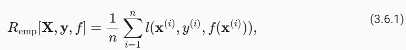
To begin with, we need to differentiate between the training error Remp, which is a statistic calculated on the training dataset, and the generalization error R, which is an expectation taken with respect to the underlying distribution. You can think of the generalization error as what you would see if you applied your model to an infinite stream of additional data examples drawn from the same underlying data distribution. Formally the training error is expressed as a sum (with the same notation as Section 3.1):
우선, 훈련 데이터세트에서 계산된 통계인 훈련 오류 Remp와 기본 분포에 대한 기대값인 일반화 오류 R을 구별해야 합니다. 일반화 오류는 동일한 기본 데이터 분포에서 추출된 추가 데이터 예제의 무한한 스트림에 모델을 적용한 경우 표시되는 오류로 생각할 수 있습니다. 공식적으로 훈련 오류는 합계로 표현됩니다(섹션 3.1과 동일한 표기법 사용).
while the generalization error is expressed as an integral:
일반화 오류는 적분으로 표현됩니다.

Problematically, we can never calculate the generalization error R exactly. Nobody ever tells us the precise form of the density function p(x,y). Moreover, we cannot sample an infinite stream of data points. Thus, in practice, we must estimate the generalization error by applying our model to an independent test set constituted of a random selection of examples X′ and labels y′ that were withheld from our training set. This consists of applying the same formula that was used for calculating the empirical training error but to a test set X′,y′.
문제는 일반화 오류 R을 정확하게 계산할 수 없다는 점입니다. 밀도 함수 p(x,y)의 정확한 형태를 알려주는 사람은 아무도 없습니다. 게다가 무한한 데이터 포인트 스트림을 샘플링할 수도 없습니다. 따라서 실제로는 훈련 세트에서 보류된 X' 및 레이블 y'의 무작위 선택으로 구성된 독립적인 테스트 세트에 모델을 적용하여 일반화 오류를 추정해야 합니다. 이는 경험적 훈련 오류를 계산하는 데 사용된 것과 동일한 공식을 테스트 세트 X',y'에 적용하는 것으로 구성됩니다.
Crucially, when we evaluate our classifier on the test set, we are working with a fixed classifier (it does not depend on the sample of the test set), and thus estimating its error is simply the problem of mean estimation. However the same cannot be said for the training set. Note that the model we wind up with depends explicitly on the selection of the training set and thus the training error will in general be a biased estimate of the true error on the underlying population. The central question of generalization is then when should we expect our training error to be close to the population error (and thus the generalization error).
결정적으로 테스트 세트에서 분류기를 평가할 때 고정된 분류기를 사용하여 작업하므로(테스트 세트의 샘플에 의존하지 않음) 오류를 추정하는 것은 단순히 평균 추정의 문제입니다. 그러나 훈련 세트에 대해서도 마찬가지입니다. 우리가 마무리하는 모델은 훈련 세트의 선택에 명시적으로 의존하므로 훈련 오류는 일반적으로 기본 모집단의 실제 오류에 대한 편향된 추정치입니다. 일반화의 핵심 질문은 언제 훈련 오류가 모집단 오류(따라서 일반화 오류)에 가까워질 것으로 예상해야 하는가입니다.
3.6.1.1. Model Complexit
In classical theory, when we have simple models and abundant data, the training and generalization errors tend to be close. However, when we work with more complex models and/or fewer examples, we expect the training error to go down but the generalization gap to grow. This should not be surprising. Imagine a model class so expressive that for any dataset of n examples, we can find a set of parameters that can perfectly fit arbitrary labels, even if randomly assigned. In this case, even if we fit our training data perfectly, how can we conclude anything about the generalization error? For all we know, our generalization error might be no better than random guessing.
고전 이론에서는 단순한 모델과 풍부한 데이터가 있을 때 훈련 및 일반화 오류가 가까운 경향이 있습니다. 그러나 더 복잡한 모델 및/또는 더 적은 수의 예제를 사용하면 학습 오류는 줄어들지만 일반화 격차는 커질 것으로 예상됩니다. 이것은 놀라운 일이 아닙니다. n개의 예제로 구성된 데이터세트에 대해 무작위로 할당되더라도 임의의 레이블에 완벽하게 맞는 매개변수 집합을 찾을 수 있을 만큼 표현력이 뛰어난 모델 클래스를 상상해 보세요. 이 경우 훈련 데이터를 완벽하게 적합하더라도 일반화 오류에 대해 어떻게 결론을 내릴 수 있습니까? 우리가 아는 한, 일반화 오류는 무작위 추측보다 나을 것이 없을 수도 있습니다.
In general, absent any restriction on our model class, we cannot conclude, based on fitting the training data alone, that our model has discovered any generalizable pattern (Vapnik et al., 1994). On the other hand, if our model class was not capable of fitting arbitrary labels, then it must have discovered a pattern. Learning-theoretic ideas about model complexity derived some inspiration from the ideas of Karl Popper, an influential philosopher of science, who formalized the criterion of falsifiability. According to Popper, a theory that can explain any and all observations is not a scientific theory at all! After all, what has it told us about the world if it has not ruled out any possibility? In short, what we want is a hypothesis that could not explain any observations we might conceivably make and yet nevertheless happens to be compatible with those observations that we in fact make.
일반적으로 모델 클래스에 대한 제한이 없으면 훈련 데이터만 피팅하는 것만으로는 모델이 일반화 가능한 패턴을 발견했다고 결론을 내릴 수 없습니다(Vapnik et al., 1994). 반면, 모델 클래스가 임의의 레이블을 맞출 수 없다면 패턴을 발견했을 것입니다. 모델 복잡성에 대한 학습 이론적인 아이디어는 반증 가능성의 기준을 공식화한 영향력 있는 과학 철학자 칼 포퍼(Karl Popper)의 아이디어에서 영감을 얻었습니다. 포퍼에 따르면, 모든 관찰을 설명할 수 있는 이론은 전혀 과학 이론이 아닙니다! 결국, 어떤 가능성도 배제하지 않는다면 세상은 우리에게 무엇을 말해주는 것일까요? 간단히 말해서, 우리가 원하는 것은 우리가 할 수 있는 어떤 관찰도 설명할 수 없지만 그럼에도 불구하고 실제로 우리가 하는 관찰과 양립할 수 있는 가설입니다.
Now what precisely constitutes an appropriate notion of model complexity is a complex matter. Often, models with more parameters are able to fit a greater number of arbitrarily assigned labels. However, this is not necessarily true. For instance, kernel methods operate in spaces with infinite numbers of parameters, yet their complexity is controlled by other means (Schölkopf and Smola, 2002). One notion of complexity that often proves useful is the range of values that the parameters can take. Here, a model whose parameters are permitted to take arbitrary values would be more complex. We will revisit this idea in the next section, when we introduce weight decay, your first practical regularization technique. Notably, it can be difficult to compare complexity among members of substantially different model classes (say, decision trees vs. neural networks).
이제 모델 복잡성에 대한 적절한 개념을 정확히 구성하는 것은 복잡한 문제입니다. 매개변수가 더 많은 모델은 임의로 할당된 레이블을 더 많이 수용할 수 있는 경우가 많습니다. 그러나 이것이 반드시 사실은 아닙니다. 예를 들어, 커널 방법은 무한한 수의 매개변수가 있는 공간에서 작동하지만 그 복잡성은 다른 수단으로 제어됩니다(Schölkopf 및 Smola, 2002). 종종 유용하다고 입증되는 복잡성에 대한 한 가지 개념은 매개변수가 취할 수 있는 값의 범위입니다. 여기서 매개변수가 임의의 값을 취하도록 허용된 모델은 더 복잡합니다. 첫 번째 실용적인 정규화 기술인 가중치 감소를 소개하는 다음 섹션에서 이 아이디어를 다시 살펴보겠습니다. 특히, 실질적으로 다른 모델 클래스(예: 의사결정 트리와 신경망)의 구성원 간의 복잡성을 비교하는 것은 어려울 수 있습니다.
At this point, we must stress another important point that we will revisit when introducing deep neural networks. When a model is capable of fitting arbitrary labels, low training error does not necessarily imply low generalization error. However, it does not necessarily imply high generalization error either! All we can say with confidence is that low training error alone is not enough to certify low generalization error. Deep neural networks turn out to be just such models: while they generalize well in practice, they are too powerful to allow us to conclude much on the basis of training error alone. In these cases we must rely more heavily on our holdout data to certify generalization after the fact. Error on the holdout data, i.e., validation set, is called the validation error.
이 시점에서 우리는 심층 신경망을 도입할 때 다시 살펴볼 또 다른 중요한 점을 강조해야 합니다. 모델이 임의의 레이블을 맞출 수 있는 경우 훈련 오류가 낮다고 해서 반드시 일반화 오류가 낮다는 의미는 아닙니다. 그러나 이것이 반드시 높은 일반화 오류를 의미하는 것은 아닙니다! 우리가 자신있게 말할 수 있는 것은 낮은 훈련 오류만으로는 낮은 일반화 오류를 인증하는 데 충분하지 않다는 것입니다. 심층 신경망은 바로 그러한 모델임이 밝혀졌습니다. 실제로는 잘 일반화되지만 훈련 오류만으로 많은 결론을 내릴 수 없을 정도로 강력합니다. 이러한 경우 사실 이후 일반화를 인증하기 위해 홀드아웃 데이터에 더 많이 의존해야 합니다. 홀드아웃 데이터, 즉 검증 세트에 대한 오류를 검증 오류라고 합니다.
3.6.2. Underfitting or Overfitting?
When we compare the training and validation errors, we want to be mindful of two common situations. First, we want to watch out for cases when our training error and validation error are both substantial but there is a little gap between them. If the model is unable to reduce the training error, that could mean that our model is too simple (i.e., insufficiently expressive) to capture the pattern that we are trying to model. Moreover, since the generalization gap (Remp−R) between our training and generalization errors is small, we have reason to believe that we could get away with a more complex model. This phenomenon is known as underfitting.
훈련 오류와 검증 오류를 비교할 때 두 가지 일반적인 상황에 유의하고 싶습니다. 먼저, 훈련 오류와 검증 오류가 모두 상당하지만 그 사이에 약간의 차이가 있는 경우를 주의하고 싶습니다. 모델이 훈련 오류를 줄일 수 없다면 이는 모델이 너무 단순하여(즉, 표현력이 부족하여) 모델링하려는 패턴을 포착할 수 없음을 의미할 수 있습니다. 더욱이 훈련 오류와 일반화 오류 사이의 일반화 격차(Remp-R)가 작기 때문에 더 복잡한 모델을 사용하여 벗어날 수 있다고 믿을 이유가 있습니다. 이 현상을 과소적합이라고 합니다.
On the other hand, as we discussed above, we want to watch out for the cases when our training error is significantly lower than our validation error, indicating severe overfitting. Note that overfitting is not always a bad thing. In deep learning especially, the best predictive models often perform far better on training data than on holdout data. Ultimately, we usually care about driving the generalization error lower, and only care about the gap insofar as it becomes an obstacle to that end. Note that if the training error is zero, then the generalization gap is precisely equal to the generalization error and we can make progress only by reducing the gap.
반면, 위에서 논의한 것처럼 훈련 오류가 검증 오류보다 현저히 낮아 심각한 과적합을 나타내는 경우를 주의해야 합니다. 과적합이 항상 나쁜 것은 아닙니다. 특히 딥 러닝에서는 최고의 예측 모델이 홀드아웃 데이터보다 훈련 데이터에서 훨씬 더 나은 성능을 발휘하는 경우가 많습니다. 궁극적으로 우리는 일반적으로 일반화 오류를 낮추는 데 관심을 갖고, 그 목적에 장애물이 되는 한 격차에만 관심을 갖습니다. 훈련 오류가 0이면 일반화 격차는 일반화 오류와 정확하게 동일하며 격차를 줄여야만 진전을 이룰 수 있습니다.
3.6.2.1. Polynomial Curve Fitting
To illustrate some classical intuition about overfitting and model complexity, consider the following: given training data consisting of a single feature x and a corresponding real-valued label y, we try to find the polynomial of degree d for estimating the label y.
과적합 및 모델 복잡성에 대한 몇 가지 고전적 직관을 설명하기 위해 다음을 고려하십시오. 단일 특성 x와 해당 실제 값 레이블 y로 구성된 훈련 데이터가 주어지면 레이블 y를 추정하기 위해 d차 다항식을 찾으려고 합니다.

This is just a linear regression problem where our features are given by the powers of x, the model’s weights are given by wi, and the bias is given by w0 since x**0=1 for all x. Since this is just a linear regression problem, we can use the squared error as our loss function.
이는 모든 x에 대해 x**0=1이므로 특성이 x의 거듭제곱으로 제공되고 모델의 가중치가 wi로 제공되며 편향이 w0으로 제공되는 선형 회귀 문제입니다. 이것은 선형 회귀 문제이므로 제곱 오차를 손실 함수로 사용할 수 있습니다.
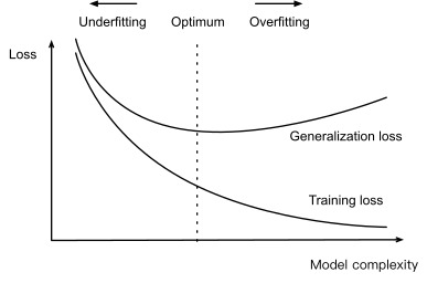
A higher-order polynomial function is more complex than a lower-order polynomial function, since the higher-order polynomial has more parameters and the model function’s selection range is wider. Fixing the training dataset, higher-order polynomial functions should always achieve lower (at worst, equal) training error relative to lower-degree polynomials. In fact, whenever each data example has a distinct value of x, a polynomial function with degree equal to the number of data examples can fit the training set perfectly. We compare the relationship between polynomial degree (model complexity) and both underfitting and overfitting in Fig. 3.6.1.
고차 다항식 함수는 저차 다항식 함수보다 더 복잡합니다. 왜냐하면 고차 다항식은 더 많은 매개변수를 갖고 모델 함수의 선택 범위가 더 넓기 때문입니다. 훈련 데이터 세트를 수정하면 고차 다항식 함수는 항상 저차 다항식에 비해 더 낮은(최악의 경우 동일한) 훈련 오류를 달성해야 합니다. 실제로 각 데이터 예제에 고유한 x 값이 있을 때마다 데이터 예제 수와 동일한 차수를 갖는 다항식 함수가 훈련 세트에 완벽하게 맞을 수 있습니다. 그림 3.6.1에서 다항식 차수(모델 복잡도)와 과소적합 및 과적합 간의 관계를 비교합니다.
3.6.2.2. Dataset Siz
As the above bound already indicates, another big consideration to bear in mind is dataset size. Fixing our model, the fewer samples we have in the training dataset, the more likely (and more severely) we are to encounter overfitting. As we increase the amount of training data, the generalization error typically decreases. Moreover, in general, more data never hurts. For a fixed task and data distribution, model complexity should not increase more rapidly than the amount of data. Given more data, we might attempt to fit a more complex model. Absent sufficient data, simpler models may be more difficult to beat. For many tasks, deep learning only outperforms linear models when many thousands of training examples are available. In part, the current success of deep learning owes considerably to the abundance of massive datasets arising from Internet companies, cheap storage, connected devices, and the broad digitization of the economy.
위의 한계에서 이미 알 수 있듯이 염두에 두어야 할 또 다른 큰 고려 사항은 데이터 세트 크기입니다. 모델을 수정하면 훈련 데이터 세트에 있는 샘플 수가 줄어들수록 과적합이 발생할 가능성이 더 높아집니다(심각하게도). 훈련 데이터의 양을 늘리면 일반적으로 일반화 오류가 감소합니다. 또한 일반적으로 더 많은 데이터가 해를 끼치 지 않습니다. 고정된 작업 및 데이터 분포의 경우 모델 복잡성이 데이터 양보다 더 빠르게 증가해서는 안 됩니다. 더 많은 데이터가 주어지면 더 복잡한 모델을 맞추려고 시도할 수도 있습니다. 데이터가 충분하지 않으면 단순한 모델을 이기기가 더 어려울 수 있습니다. 많은 작업에서 딥 러닝은 수천 개의 학습 예제를 사용할 수 있는 경우에만 선형 모델보다 성능이 뛰어납니다. 부분적으로 현재 딥 러닝의 성공은 인터넷 회사, 저렴한 스토리지, 연결된 장치 및 경제의 광범위한 디지털화에서 발생하는 풍부한 대규모 데이터 세트에 크게 기인합니다.
3.6.3. Model Selection
Typically, we select our final model only after evaluating multiple models that differ in various ways (different architectures, training objectives, selected features, data preprocessing, learning rates, etc.). Choosing among many models is aptly called model selection.
일반적으로 우리는 다양한 방식(다양한 아키텍처, 교육 목표, 선택한 기능, 데이터 전처리, 학습 속도 등)이 다른 여러 모델을 평가한 후에만 최종 모델을 선택합니다. 여러 모델 중에서 선택하는 것을 적절하게는 모델 선택이라고 합니다.
In principle, we should not touch our test set until after we have chosen all our hyperparameters. Were we to use the test data in the model selection process, there is a risk that we might overfit the test data. Then we would be in serious trouble. If we overfit our training data, there is always the evaluation on test data to keep us honest. But if we overfit the test data, how would we ever know? See Ong et al. (2005) for an example of how this can lead to absurd results even for models where the complexity can be tightly controlled.
원칙적으로 모든 하이퍼파라미터를 선택할 때까지 테스트 세트를 건드리면 안 됩니다. 모델 선택 과정에서 테스트 데이터를 사용한다면 테스트 데이터에 과적합될 위험이 있습니다. 그러면 우리는 심각한 문제에 빠지게 될 것입니다. 훈련 데이터를 과대적합하는 경우 정직성을 유지하기 위해 항상 테스트 데이터에 대한 평가가 있습니다. 하지만 테스트 데이터에 과대적합되면 어떻게 알 수 있을까요? Ong et al. (2005)은 복잡성이 엄격하게 제어될 수 있는 모델의 경우에도 이것이 어떻게 터무니없는 결과로 이어질 수 있는지에 대한 예를 제공합니다.
Thus, we should never rely on the test data for model selection. And yet we cannot rely solely on the training data for model selection either because we cannot estimate the generalization error on the very data that we use to train the model.
따라서 모델 선택을 위해 테스트 데이터에 의존해서는 안 됩니다. 그러나 모델을 훈련하는 데 사용하는 바로 그 데이터에 대한 일반화 오류를 추정할 수 없기 때문에 모델 선택을 위해 훈련 데이터에만 의존할 수는 없습니다.
In practical applications, the picture gets muddier. While ideally we would only touch the test data once, to assess the very best model or to compare a small number of models with each other, real-world test data is seldom discarded after just one use. We can seldom afford a new test set for each round of experiments. In fact, recycling benchmark data for decades can have a significant impact on the development of algorithms, e.g., for image classification and optical character recognition.
실제 적용에서는 그림이 더 흐릿해집니다. 이상적으로는 테스트 데이터를 한 번만 만지는 반면, 최고의 모델을 평가하거나 소수의 모델을 서로 비교하기 위해 실제 테스트 데이터는 한 번만 사용한 후 거의 삭제되지 않습니다. 우리는 각 실험 라운드마다 새로운 테스트 세트를 제공할 여력이 거의 없습니다. 실제로 수십 년 동안 벤치마크 데이터를 재활용하면 이미지 분류, 광학 문자 인식 등의 알고리즘 개발에 상당한 영향을 미칠 수 있습니다.
The common practice for addressing the problem of training on the test set is to split our data three ways, incorporating a validation set in addition to the training and test datasets. The result is a murky business where the boundaries between validation and test data are worryingly ambiguous. Unless explicitly stated otherwise, in the experiments in this book we are really working with what should rightly be called training data and validation data, with no true test sets. Therefore, the accuracy reported in each experiment of the book is really the validation accuracy and not a true test set accuracy.
테스트 세트에 대한 교육 문제를 해결하기 위한 일반적인 방법은 데이터를 세 가지 방식으로 분할하고 교육 및 테스트 데이터세트 외에 검증 세트를 통합하는 것입니다. 그 결과 검증 데이터와 테스트 데이터 사이의 경계가 걱정스러울 정도로 모호한 비즈니스가 불투명해졌습니다. 달리 명시적으로 언급하지 않는 한, 이 책의 실험에서 우리는 실제 테스트 세트 없이 훈련 데이터와 검증 데이터라고 해야 할 것을 실제로 사용하고 있습니다. 따라서 책의 각 실험에서 보고된 정확도는 실제 검증 정확도이지 실제 테스트 세트 정확도가 아닙니다.
3.6.3.1. Cross-Validation
When training data is scarce, we might not even be able to afford to hold out enough data to constitute a proper validation set. One popular solution to this problem is to employ K-fold cross-validation. Here, the original training data is split into K non-overlapping subsets. Then model training and validation are executed K times, each time training on K −1 subsets and validating on a different subset (the one not used for training in that round). Finally, the training and validation errors are estimated by averaging over the results from the K experiments.
훈련 데이터가 부족하면 적절한 검증 세트를 구성하기에 충분한 데이터를 보유할 여력조차 없을 수도 있습니다. 이 문제에 대한 인기 있는 해결책 중 하나는 K-겹 교차 검증을 사용하는 것입니다. 여기서는 원본 훈련 데이터가 K개의 겹치지 않는 하위 집합으로 분할됩니다. 그런 다음 모델 훈련 및 검증이 K번 실행되며, 매번 K −1 하위 집합에 대해 훈련하고 다른 하위 집합(해당 라운드에서 훈련에 사용되지 않은 것)에 대해 검증합니다. 마지막으로 훈련 및 검증 오류는 K 실험 결과를 평균하여 추정됩니다.
3.6.4. Summary
This section explored some of the underpinnings of generalization in machine learning. Some of these ideas become complicated and counterintuitive when we get to deeper models; here, models are capable of overfitting data badly, and the relevant notions of complexity can be both implicit and counterintuitive (e.g., larger architectures with more parameters generalizing better). We leave you with a few rules of thumb:
이 섹션에서는 기계 학습에서 일반화의 몇 가지 토대를 살펴보았습니다. 이러한 아이디어 중 일부는 더 심층적인 모델에 도달하면 복잡해지고 직관에 반하게 됩니다. 여기서 모델은 데이터를 잘못 과적합할 수 있으며 관련 복잡성 개념은 암시적일 수도 있고 반직관적일 수도 있습니다(예: 더 많은 매개변수를 가진 더 큰 아키텍처가 더 잘 일반화됨). 몇 가지 경험 법칙을 알려드리겠습니다.
- Use validation sets (or K-fold cross-validation) for model selection;
모델 선택을 위해 검증 세트(또는 K-겹 교차 검증)를 사용합니다. - More complex models often require more data;
더 복잡한 모델에는 더 많은 데이터가 필요한 경우가 많습니다. - Relevant notions of complexity include both the number of parameters and the range of values that they are allowed to take;
복잡성과 관련된 개념에는 매개변수의 수와 허용되는 값의 범위가 모두 포함됩니다. - Keeping all else equal, more data almost always leads to better generalization;
다른 모든 것을 동일하게 유지하면 더 많은 데이터가 거의 항상 더 나은 일반화로 이어집니다. - This entire talk of generalization is all predicated on the IID assumption. If we relax this assumption, allowing for distributions to shift between the train and testing periods, then we cannot say anything about generalization absent a further (perhaps milder) assumption.
일반화에 대한 이 전체 이야기는 모두 IID 가정에 근거합니다. 이 가정을 완화하여 열차와 테스트 기간 사이에 분포가 이동하도록 허용하면 추가(아마도 더 온화한) 가정 없이 일반화에 대해 아무 말도 할 수 없습니다.
3.6.5. Exercises
- When can you solve the problem of polynomial regression exactly?
- Give at least five examples where dependent random variables make treating the problem as IID data inadvisable.
- Can you ever expect to see zero training error? Under which circumstances would you see zero generalization error?
- Why is K -fold cross-validation very expensive to compute?
- Why is the K -fold cross-validation error estimate biased?
- The VC dimension is defined as the maximum number of points that can be classified with arbitrary labels {±1} by a function of a class of functions. Why might this not be a good idea for measuring how complex the class of functions is? Hint: consider the magnitude of the functions.
- Your manager gives you a difficult dataset on which your current algorithm does not perform so well. How would you justify to him that you need more data? Hint: you cannot increase the data but you can decrease it.
'Dive into Deep Learning > D2L Linear Neural Networks' 카테고리의 다른 글
| D2L - 3.7. Weight Decay (1) | 2023.12.03 |
|---|---|
| D2L - 4.7. Environment and Distribution Shift (0) | 2023.06.27 |
| D2L - 4.6. Generalization in Classification (0) | 2023.06.27 |
| D2L - 4.5. Concise Implementation of Softmax Regression¶ (0) | 2023.06.27 |
| D2L - 4.4. Softmax Regression Implementation from Scratch (0) | 2023.06.26 |
| D2L - 4.3. The Base Classification Model (0) | 2023.06.26 |
| D2L - 4.2. The Image Classification Dataset (0) | 2023.06.26 |
| D2L 4.1. Softmax Regression (0) | 2023.06.26 |
| D2L - 4. Linear Neural Networks for Classification (0) | 2023.06.26 |
| D2L - Local Environment Setting (0) | 2023.06.26 |