
https://d2l.ai/chapter_linear-classification/softmax-regression-concise.html
4.5. Concise Implementation of Softmax Regression — Dive into Deep Learning 1.0.0-beta0 documentation
d2l.ai
4.5. Concise Implementation of Softmax Regression
Just as high-level deep learning frameworks made it easier to implement linear regression (see Section 3.5), they are similarly convenient here.
high-level deep learning frameworks -고급 딥 러닝 프레임워크-가 linear regression -선형 회귀- 구현을 더 쉽게 만든 것처럼(섹션 3.5 참조) 여기서도 마찬가지로 편리합니다.
import torch
from torch import nn
from torch.nn import functional as F
from d2l import torch as d2l
위의 코드는 PyTorch와 d2l 라이브러리에서 사용되는 모듈들을 임포트하는 과정을 나타냅니다. 코드를 한 줄씩 설명해드리겠습니다.
- import torch: PyTorch 라이브러리를 임포트합니다. PyTorch는 딥러닝 모델을 구성하고 학습하는 데 사용되는 라이브러리입니다.
- from torch import nn: torch.nn 모듈을 임포트합니다. torch.nn은 신경망 모델을 구성하는 데 필요한 다양한 클래스와 함수들을 제공합니다.
- from torch.nn import functional as F: torch.nn.functional 모듈을 임포트하고, 이를 F라는 별칭으로 사용할 수 있도록 합니다. torch.nn.functional은 활성화 함수, 손실 함수, 정규화 함수 등과 같은 다양한 함수들을 제공합니다.
- from d2l import torch as d2l: d2l 패키지의 torch 모듈을 임포트하고, 이를 d2l이라는 별칭으로 사용할 수 있도록 합니다. d2l은 Dive into Deep Learning (D2L) 책의 예제 코드와 유틸리티 함수를 제공하는 라이브러리입니다.
위의 코드는 PyTorch와 d2l 라이브러리에서 제공되는 모듈들을 현재 환경에 가져와서 사용할 수 있도록 하는 과정을 수행합니다.
4.5.1. Defining the Model
As in Section 3.5, we construct our fully connected layer using the built-in layer. The built-in __call__ method then invokes forward whenever we need to apply the network to some input.
섹션 3.5에서와 같이 built-in layer -내장 계층-을 사용하여 fully connected layer-완전 연결 계층-을 구성합니다. built-in __call__ method -내장된 __call__ 메서드-는 네트워크를 일부 입력에 적용해야 할 때마다 호출합니다.
We use a Flatten layer to convert the 4th order tensor X to 2nd order by keeping the dimensionality along the first axis unchanged.
Flatten 레이어를 사용하여 첫 번째 axis -축-을 따라 차원을 변경하지 않고 유지함으로써 4th order tensor X -4차 텐서 X-를 2nd order -2차-로 변환합니다.
class SoftmaxRegression(d2l.Classifier):  #@save
    """The softmax regression model."""
    def __init__(self, num_outputs, lr):
        super().__init__()
        self.save_hyperparameters()
        self.net = nn.Sequential(nn.Flatten(),
                                 nn.LazyLinear(num_outputs))

    def forward(self, X):
        return self.net(X)
위의 코드는 softmax 회귀(Softmax Regression) 모델을 정의하는 클래스인 SoftmaxRegression을 나타냅니다. 코드를 한 줄씩 설명해드리겠습니다.
- class SoftmaxRegression(d2l.Classifier):: SoftmaxRegression 클래스를 정의합니다. 이 클래스는 d2l.Classifier를 상속받습니다. d2l.Classifier는 분류 모델의 기본 클래스로서, 분류 모델에서 공통적으로 사용되는 기능을 제공합니다.
- def __init__(self, num_outputs, lr):: SoftmaxRegression 클래스의 생성자 함수입니다. num_outputs와 lr을 인자로 받습니다. num_outputs는 출력의 개수를 나타내며, lr은 학습률(learning rate)을 나타냅니다.
- super().__init__(): 상위 클래스인 d2l.Classifier의 생성자를 호출합니다.
- self.save_hyperparameters(): 모델의 하이퍼파라미터를 저장합니다. num_outputs와 lr을 저장합니다.
- self.net = nn.Sequential(nn.Flatten(), nn.LazyLinear(num_outputs)): nn.Sequential을 사용하여 모델의 신경망을 정의합니다. nn.Flatten()은 입력 데이터를 1차원으로 펼치는 역할을 합니다. nn.LazyLinear(num_outputs)는 선형 변환을 수행하는 레이어로서, 입력의 크기를 num_outputs로 변환합니다.
- def forward(self, X):: 모델의 순전파(forward pass) 연산을 수행하는 함수입니다. X를 입력으로 받고, self.net(X)를 통해 신경망을 통과시킨 결과를 반환합니다. self.net(X)는 입력 X를 nn.Sequential에 따라 순차적으로 처리하여 출력을 계산합니다.
위의 코드는 softmax 회귀 모델을 정의하는 클래스입니다. SoftmaxRegression 클래스는 d2l.Classifier를 상속받아 분류 모델의 공통 기능을 활용하며, nn.Sequential을 사용하여 모델의 신경망을 정의합니다. 순전파 연산은 forward 함수에서 수행되며, 입력 데이터를 신경망에 통과시켜 출력을 계산합니다.
4.5.2. Softmax Revisited
In Section 4.4 we calculated our model’s output and applied the cross-entropy loss. While this is perfectly reasonable mathematically, it is risky computationally, due to numerical underflow and overflow in the exponentiation.
섹션 4.4에서 모델의 출력을 계산하고 cross-entropy loss -교차 엔트로피 손실-을 적용했습니다. 이것은 수학적으로는 완벽하게 타당하지만 exponentiation -지수화-의 numerical underflow -수치적 언더플로- 및 overflow -오버플로-로 인해 computationally -계산적으로는- risky -위험-합니다.
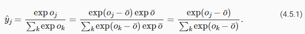
Recall that the softmax function computes probabilities via y^j=exp(oj)∑kexp(ok). If some of the 'ok' are very large, i.e., very positive, then exp(ok) might be larger than the largest number we can have for certain data types. This is called overflow. Likewise, if all arguments are very negative, we will get underflow. For instance, single precision floating point numbers approximately cover the range of 10−38 to 1038. As such, if the largest term in o lies outside the interval [−90,90], the result will not be stable. A solution to this problem is to subtract o¯=def maxkok from all entries:
softmax 함수는 y^j=exp(oj)∑kexp(ok)를 통해 확률을 계산합니다. 'ok' 중 일부가 매우 큰 경우(즉, 매우 양수인 경우) exp(ok)는 특정 데이터 유형에 대해 가질 수 있는 최대 수보다 클 수 있습니다. 이를 overflow -오버플로-라고 합니다. 마찬가지로 모든 인수가 매우 negative면 underflow -언더플로-가 발생합니다. 예를 들어 single precision floating point numbers -단정밀도 부동 소수점 숫자-는 대략 10 윗첨자−38에서 10 윗첨자 38 범위를 포함합니다. 따라서 o의 가장 큰 항이 구간 [−90,90] 밖에 있는 경우 결과가 안정적이지 않습니다. 이 문제에 대한 해결책은 모든 항목에서 o¯=def maxkok를 빼는 것입니다.
By construction we know that oj−o¯≤ 0 for all j. As such, for a q-class classification problem, the denominator is contained in the interval [1,q]. Moreover, the numerator never exceeds 1, thus preventing numerical overflow. Numerical underflow only occurs when exp(oj−o¯) numerically evaluates as 0. Nonetheless, a few steps down the road we might find ourselves in trouble when we want to compute logy^j as log 0. In particular, in backpropagation, we might find ourselves faced with a screenful of the dreaded NaN (Not a Number) results.
By construction -구성에 의해- 우리는 모든 j에 대해 oj-o̅≤ 0임을 압니다. 따라서 q-class classification problem -q 클래스 분류 문제-의 경우 denominator -분모-는 interval -구간- [1,q]에 포함됩니다. 또한 numerator -분자-는 1을 초과하지 않으므로 numerical overflow -숫자 오버플로-를 방지합니다. 수치적 언더플로는 exp(oj−o¯)가 수치적으로 0으로 평가될 때만 발생합니다. 그럼에도 불구하고, logy^j를 log 0으로 계산하려고 할 때 문제가 발생할 수 있습니다. 특히, backpropagation -역전파-에서 우리는 두려운 NaN(숫자가 아님) 결과의 화면 전체에 직면할 수 있습니다.
Fortunately, we are saved by the fact that even though we are computing exponential functions, we ultimately intend to take their log (when calculating the cross-entropy loss). By combining softmax and cross-entropy, we can escape the numerical stability issues altogether. We have:
다행스럽게도 우리는 exponential functions -지수 함수-를 계산하고 있지만 궁극적으로 log -로그-를 취하려고 한다는 것(교차 엔트로피 손실을 계산할 때)을 알고 있습니다. softmax -소프트맥스-와 cross-entropy -교차 엔트로피-를 결합하면 numerical stability issues -수치적 안정성 문제-를 모두 피할 수 있습니다. 이는 다음과 같이 표현 합니다.
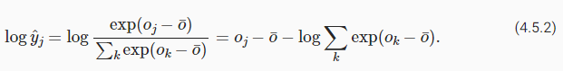
This avoids both overflow and underflow. We will want to keep the conventional softmax function handy in case we ever want to evaluate the output probabilities by our model. But instead of passing softmax probabilities into our new loss function, we just pass the logits and compute the softmax and its log all at once inside the cross-entropy loss function, which does smart things like the “LogSumExp trick”.
이것은 overflow 와 underflow를 모두 방지합니다. 모델의 output probabilities -출력 확률-을 평가하려는 경우에 대비하여 기존의 conventional softmax function을 유지하려고 합니다. 그러나 softmax probabilities -소프트맥스 확률-을 새로운 loss function -손실 함수-에 전달하는 대신, 우리는 logits -로짓-을 전달하고 "LogSumExp trick"과 같은 스마트한 작업을 수행하는 cross-entropy loss function -교차 엔트로피 손실 함수- 내부에서 softmax -소프트맥스-와 해당 log -로그-를 모두 한 번에 계산합니다.
@d2l.add_to_class(d2l.Classifier)  #@save
def loss(self, Y_hat, Y, averaged=True):
    Y_hat = Y_hat.reshape((-1, Y_hat.shape[-1]))
    Y = Y.reshape((-1,))
    return F.cross_entropy(
        Y_hat, Y, reduction='mean' if averaged else 'none')
위의 코드는 d2l.Classifier 클래스에 loss 메서드를 추가하는 코드입니다. 코드를 한 줄씩 설명하겠습니다.
- @d2l.add_to_class(d2l.Classifier): d2l.Classifier 클래스에 메서드를 추가하기 위해 데코레이터(@d2l.add_to_class)를 사용합니다.
- def loss(self, Y_hat, Y, averaged=True):: loss 메서드를 정의합니다. 이 메서드는 Y_hat과 Y를 인자로 받으며, averaged는 평균화 여부를 나타내는 불리언 매개변수입니다. Y_hat은 모델의 출력값이고, Y는 정답 레이블입니다.
- Y_hat = Y_hat.reshape((-1, Y_hat.shape[-1])): Y_hat을 2차원으로 재구성합니다. -1은 해당 차원의 크기를 자동으로 계산하라는 의미입니다. Y_hat의 마지막 차원의 크기는 클래스의 개수를 나타냅니다.
- Y = Y.reshape((-1,)): Y를 1차원으로 재구성합니다.
- return F.cross_entropy(Y_hat, Y, reduction='mean' if averaged else 'none'): F.cross_entropy 함수를 사용하여 크로스 엔트로피 손실을 계산합니다. Y_hat은 모델의 출력값, Y는 정답 레이블을 나타냅니다. reduction 매개변수를 통해 손실의 계산 방식을 설정할 수 있으며, mean은 평균을 구하고 none은 평균을 구하지 않는 옵션입니다.
위의 코드는 d2l.Classifier 클래스에 loss 메서드를 추가합니다. 이 메서드는 크로스 엔트로피 손실을 계산하는 역할을 수행합니다. 손실을 계산할 때는 모델의 출력값 Y_hat과 정답 레이블 Y을 사용하며, 평균화 여부에 따라 손실을 계산합니다.
4.5.3. Training
Next we train our model. We use Fashion-MNIST images, flattened to 784-dimensional feature vectors.
다음으로 모델을 훈련합니다. 784차원 특징 벡터로 평면화된 Fashion-MNIST 이미지를 사용합니다.
data = d2l.FashionMNIST(batch_size=256)
model = SoftmaxRegression(num_outputs=10, lr=0.1)
trainer = d2l.Trainer(max_epochs=10)
trainer.fit(model, data)
위의 코드는 FashionMNIST 데이터셋으로 Softmax 회귀 모델을 학습하는 과정을 나타내고 있습니다. 코드를 한 줄씩 설명하겠습니다.
- data = d2l.FashionMNIST(batch_size=256): d2l.FashionMNIST 클래스의 인스턴스를 생성하여 데이터를 로드합니다. batch_size는 한 번에 처리할 미니배치의 크기입니다.
- model = SoftmaxRegression(num_outputs=10, lr=0.1): SoftmaxRegression 클래스의 인스턴스를 생성하여 Softmax 회귀 모델을 초기화합니다. num_outputs은 출력 클래스의 개수이고, lr은 학습률(learning rate)입니다.
- trainer = d2l.Trainer(max_epochs=10): d2l.Trainer 클래스의 인스턴스를 생성합니다. max_epochs는 최대 에포크(epoch) 수를 나타내며, 한 에포크는 전체 데이터셋에 대해 한 번의 순회를 의미합니다.
- trainer.fit(model, data): trainer를 사용하여 모델을 학습합니다. model은 학습할 모델을, data는 학습에 사용할 데이터셋을 의미합니다.
위의 코드는 FashionMNIST 데이터셋을 사용하여 Softmax 회귀 모델을 학습하는 과정을 나타내고 있습니다. Trainer를 사용하여 모델을 학습하면서 에포크마다 손실과 정확도를 출력하고, 최대 에포크 수에 도달하거나 학습이 조기 종료될 때까지 반복적으로 모델을 학습합니다.
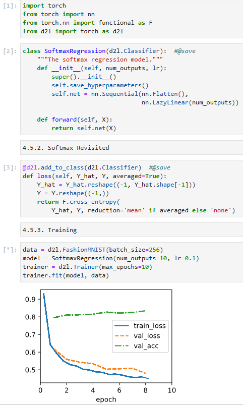
As before, this algorithm converges to a solution that achieves a decent accuracy, albeit this time with fewer lines of code than before.
이전과 마찬가지로 이 알고리즘은 이번에는 이전보다 적은 코드 줄이지만 적절한 정확도를 달성하는 솔루션으로 수렴됩니다.
4.5.4. Summary
High-level APIs are very convenient at hiding potentially dangerous aspects from their user, such as numerical stability. Moreover, they allow users to design models concisely with very few lines of code. This is both a blessing and a curse. The obvious benefit is that it makes things highly accessible, even to engineers who never took a single class of statistics in their life (in fact, this is one of the target audiences of the book). But hiding the sharp edges also comes with a price: a disincentive to add new and different components on your own, since there’s little muscle memory for doing it. Moreover, it makes it more difficult to fix things whenever the protective padding of a framework fails to cover all the corner cases entirely. Again, this is due to lack of familiarity.
높은 수준의 API는 수치 안정성과 같이 잠재적으로 위험한 측면을 사용자에게 숨기는 데 매우 편리합니다. 또한 사용자는 매우 적은 수의 코드로 간결하게 모델을 설계할 수 있습니다. 이것은 축복이자 저주입니다. 명백한 이점은 평생 통계학 수업을 한 번도 들어본 적이 없는 엔지니어도 쉽게 접근할 수 있다는 것입니다(사실 이 책의 대상 독자 중 하나입니다). 그러나 날카로운 모서리를 숨기는 데는 대가가 따릅니다. 새롭고 다양한 구성 요소를 직접 추가하는 데 필요한 근육 기억력이 거의 없기 때문에 의욕이 없습니다. 게다가 프레임워크의 보호 패딩이 모든 코너 케이스를 완전히 덮지 못할 때마다 문제를 해결하기가 더 어려워집니다. 다시 말하지만 이것은 친숙함이 부족하기 때문입니다.
As such, we strongly urge you to review both the bare bones and the elegant versions of many of the implementations that follow. While we emphasize ease of understanding, the implementations are nonetheless usually quite performant (convolutions are the big exception here). It is our intention to allow you to build on these when you invent something new that no framework can give you.
따라서 다음 구현의 bare bones -베어본-과 elegant versions -우아한 버전-을 모두 검토할 것을 강력히 촉구합니다. 우리는 이해의 용이성을 강조하지만 그럼에도 불구하고 구현은 일반적으로 상당히 성능이 좋습니다(여기서 컨볼루션은 큰 예외입니다). 프레임워크가 제공할 수 없는 새로운 것을 발명할 때 이를 기반으로 구축할 수 있도록 하는 것이 우리의 의도입니다.
4.5.5. Exercises
- Deep learning uses many different number formats, including FP64 double precision (used extremely rarely), FP32 single precision, BFLOAT16 (good for compressed representations), FP16 (very unstable), TF32 (a new format from NVIDIA), and INT8. Compute the smallest and largest argument of the exponential function for which the result does not lead to a numerical underflow or overflow.
- INT8 is a very limited format with nonzero numbers from 1 to 255. How could you extend its dynamic range without using more bits? Do standard multiplication and addition still work?
- Increase the number of epochs for training. Why might the validation accuracy decrease after a while? How could we fix this?
- What happens as you increase the learning rate? Compare the loss curves for several learning rates. Which one works better? When?
'Dive into Deep Learning > D2L Linear Neural Networks' 카테고리의 다른 글
| D2L - 3.7. Weight Decay (1) | 2023.12.03 |
|---|---|
| D2L - 3.6. Generalization (1) | 2023.12.03 |
| D2L - 4.7. Environment and Distribution Shift (0) | 2023.06.27 |
| D2L - 4.6. Generalization in Classification (0) | 2023.06.27 |
| D2L - 4.4. Softmax Regression Implementation from Scratch (0) | 2023.06.26 |
| D2L - 4.3. The Base Classification Model (0) | 2023.06.26 |
| D2L - 4.2. The Image Classification Dataset (0) | 2023.06.26 |
| D2L 4.1. Softmax Regression (0) | 2023.06.26 |
| D2L - 4. Linear Neural Networks for Classification (0) | 2023.06.26 |
| D2L - Local Environment Setting (0) | 2023.06.26 |