

https://d2l.ai/chapter_linear-classification/generalization-classification.html
4.6. Generalization in Classification — Dive into Deep Learning 1.0.0-beta0 documentation
d2l.ai
4.6. Generalization in Classification
So far, we have focused on how to tackle multiclass classification problems by training (linear) neural networks with multiple outputs and softmax functions. Interpreting our model’s outputs as probabilistic predictions, we motivated and derived the cross-entropy loss function, which calculates the negative log likelihood that our model (for a fixed set of parameters) assigns to the actual labels. And finally, we put these tools into practice by fitting our model to the training set. However, as always, our goal is to learn general patterns, as assessed empirically on previously unseen data (the test set). High accuracy on the training set means nothing. Whenever each of our inputs is unique (and indeed this is true for most high-dimensional datasets), we can attain perfect accuracy on the training set by just memorizing the dataset on the first training epoch, and subsequently looking up the label whenever we see a new image. And yet, memorizing the exact labels associated with the exact training examples does not tell us how to classify new examples. Absent further guidance, we might have to fall back on random guessing whenever we encounter new examples.
지금까지 우리는 다중 출력 및 softmax 함수를 사용하여 (선형) 신경망을 훈련하여 다중 클래스 분류 문제를 해결하는 방법에 중점을 두었습니다. 모델의 출력을 확률적 예측으로 해석하여 모델(매개 변수의 고정 세트에 대해)이 실제 레이블에 할당하는 음의 로그 우도를 계산하는 교차 엔트로피 손실 함수에 동기를 부여하고 도출했습니다. 마지막으로 모델을 교육 세트에 맞춰 이러한 도구를 실행합니다. 그러나 항상 그렇듯이 우리의 목표는 이전에 본 적이 없는 데이터(테스트 세트)에서 경험적으로 평가되는 일반적인 패턴을 학습하는 것입니다. 훈련 세트의 높은 정확도는 아무 의미가 없습니다. 각 입력이 고유할 때마다(실제로 이것은 대부분의 고차원 데이터 세트에 해당됨) 첫 번째 교육 에포크에서 데이터 세트를 기억하고 이후 볼 때마다 레이블을 조회하여 교육 세트에서 완벽한 정확도를 얻을 수 있습니다. 새로운 이미지. 그러나 정확한 훈련 예제와 관련된 정확한 레이블을 기억하는 것은 새로운 예제를 분류하는 방법을 알려주지 않습니다. 추가 지침이 없으면 새로운 예를 만날 때마다 무작위 추측에 의존해야 할 수도 있습니다.
A number of burning questions demand immediate attention:
즉각적인 주의를 요하는 수많은 질문이 있습니다.
- How many test examples do we need to precisely estimate the accuracy of our classifiers on the underlying population?
기본 모집단에 대한 분류기의 정확도를 정확하게 추정하려면 몇 개의 테스트 예제가 필요합니까? - What happens if we keep evaluating models on the same test repeatedly?
동일한 테스트에서 모델을 반복적으로 평가하면 어떻게 될까요? - Why should we expect that fitting our linear models to the training set should fare any better than our naive memorization scheme?
훈련 세트에 선형 모델을 맞추는 것이 순진한 암기 체계보다 나은 결과를 얻을 수 있는 이유는 무엇입니까?
While Section 3.6 introduced the basics of overfitting and generalization in the context of linear regression, this chapter will go a little deeper, introducing some of the foundational ideas of statistical learning theory. It turns out that we often can guarantee generalization a priori: for many models, and for any desired upper bound on the generalization gap E, we can often determine some required number of samples n such that if our training set contains at least n samples, then our empirical error will lie within E of the true error, for any data generating distribution. Unfortunately, it also turns out that while these sorts of guarantees provide a profound set of intellectual building blocks, they are of limited practical utility to the deep learning practitioner. In short, these guarantees suggest that ensuring generalization of deep neural networks a priori requires an absurd number of examples (perhaps trillions or more), even when we find that, on the tasks we care about, deep neural networks typically generalize remarkably well with far fewer examples (thousands). Thus deep learning practitioners often forgo a priori guarantees altogether, instead employing methods on the basis that they have generalized well on similar problems in the past, and certifying generalization post hoc through empirical evaluations. When we get to Section 5, we will revisit generalization and provide a light introduction to the vast scientific literature that has sprung in attempts to explain why deep neural networks generalize in practice.
섹션 3.6에서 선형 회귀의 맥락에서 과대적합 및 일반화의 기본 사항을 소개했지만 이 장에서는 통계 학습 이론의 기본 아이디어 중 일부를 소개하면서 조금 더 깊이 들어갈 것입니다. 우리는 종종 일반화를 선험적으로 보장할 수 있음이 밝혀졌습니다. 많은 모델에 대해, 그리고 일반화 갭 E의 원하는 상한에 대해 훈련 세트가 적어도 n 샘플을 포함하는 경우 필요한 샘플 수 n을 종종 결정할 수 있습니다. 그러면 우리의 경험적 오류는 모든 데이터 생성 분포에 대해 실제 오류의 E 내에 있을 것입니다. 불행하게도 이러한 종류의 보증은 심오한 지적 구성 요소 세트를 제공하지만 딥 러닝 실무자에게 실질적인 유용성은 제한적입니다. 요컨대, 이러한 보장은 심층 신경망의 일반화를 보장하려면 터무니없는 수의 예(아마도 수조 개 이상)가 필요하다는 것을 시사합니다. 더 적은 예(수천). 따라서 딥 러닝 실무자는 종종 선험적 보장을 모두 포기하고 대신 과거에 비슷한 문제에 대해 잘 일반화했다는 기반의 방법을 사용하고 경험적 평가를 통해 사후 일반화를 인증합니다. 섹션 5에서는 일반화를 다시 살펴보고 심층 신경망이 실제로 일반화되는 이유를 설명하려는 시도에서 생겨난 방대한 과학 문헌에 대한 간단한 소개를 제공합니다.
4.6.1. The Test Set
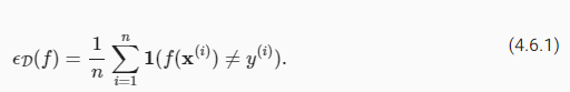
Since we have already begun to rely on test sets as the gold standard method for assessing generalization error, let’s get started by discussing the properties of such error estimates. Let’s focus on a fixed classifier f, without worrying about how it was obtained. Moreover suppose that we possess a fresh dataset of examples D=(x(i),y(i))ni=1 that were not used to train the classifier f. The empirical error of our classifier f on D is simply the fraction of instances for which the prediction f(x(i)) disagrees with the true label y(i), and is given by the following expression:
우리는 이미 일반화 오류를 평가하기 위한 표준 방법으로 테스트 세트에 의존하기 시작했기 때문에 이러한 오류 추정의 속성에 대해 논의하는 것으로 시작하겠습니다. 어떻게 획득했는지 걱정하지 않고 고정된 분류자 f에 초점을 맞추겠습니다. 또한 분류기 f를 훈련하는 데 사용되지 않은 예제 D=(x(i),y(i))ni=1의 새로운 데이터 세트를 보유하고 있다고 가정합니다. D에 대한 분류자 f의 경험적 오류는 단순히 예측 f(x(i))가 실제 레이블 y(i)와 일치하지 않는 인스턴스의 비율이며 다음 식으로 제공됩니다.
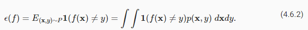
By contrast, the population error is the expected fraction of examples in the underlying population (some distribution P(X,Y) characterized by probability density function p(x,y)) for which our classifier disagrees with the true label:
대조적으로, 모집단 오류는 기본 모집단(확률 밀도 함수 p(x,y)로 특징지어지는 일부 분포 P(X,Y))에서 분류기가 실제 레이블과 일치하지 않는 예상되는 예의 비율입니다.
While E(f) is the quantity that we actually care about, we cannot observe it directly, just as we cannot directly observe the average height in a large population without measuring every single person. We can only estimate this quantity based on samples. Because our test set D is statistically representative of the underlying population, we can view ED(f) as a statistical estimator of the population error E(f). Moreover, because our quantity of interest E(f) is an expectation (of the random variable 1(f(X)≠Y)) and the corresponding estimator ED(f) is the sample average, estimating the population error is simply the classic problem of mean estimation, which you may recall from Section 2.6.
E(f)는 우리가 실제로 관심을 갖는 양이지만 모든 사람을 측정하지 않고는 대규모 인구의 평균 키를 직접 관찰할 수 없는 것처럼 직접 관찰할 수 없습니다. 샘플을 기반으로 이 수량만 추정할 수 있습니다. 테스트 세트 D는 기본 모집단을 통계적으로 대표하므로 ED(f)를 모집단 오류 E(f)의 통계적 추정기로 볼 수 있습니다. 게다가 our quantity of interest E(f)는 expectation (of the random variable 1(f(X)≠Y)) 입니다. 그리고 corresponding estimator ED(f)는 표본 평균이며, estimating the population error 는 간단한 mean estimation의 classic problem 입니다.이는 Section 2.6. 에서 다루었었습니다.
An important classical result from probability theory called the central limit theorem guarantees that whenever we possess n random samples a1,...,an drawn from any distribution with mean u and standard deviation a, as the number of samples n approaches infinity, the sample average u^ approximately tends towards a normal distribution centered at the true mean and with standard deviation a/root n. Already, this tells us something important: as the number of examples grows large, our test error ED(f) should approach the true error E(f) at a rate of O(1/root n). Thus, to estimate our test error twice as precisely, we must collect four times as large a test set. To reduce our test error by a factor of one hundred, we must collect ten thousand times as large a test set. In general, such a rate of O(1/root n) is often the best we can hope for in statistics.
중앙 극한 정리(central limit theorem)라고 하는 확률 이론의 중요한 고전적 결과는 평균 u 및 표준 편차 a를 갖는 임의의 분포에서 추출된 n개의 무작위 샘플 a1,...an을 가질 때마다 샘플 수 n이 무한대에 접근할 때 샘플이 평균 u^은 대략 참 평균에 중심을 두고 표준 편차 a/root n을 갖는 정규 분포를 향하는 경향이 있습니다. 이미 이것은 우리에게 중요한 사실을 알려줍니다. 예의 수가 커짐에 따라 테스트 오류 ED(f)는 O(1/root n)의 비율로 실제 오류 E(f)에 접근해야 합니다. 따라서 테스트 오류를 두 배 더 정확하게 추정하려면 테스트 세트를 네 배 더 수집해야 합니다. 테스트 오류를 100분의 1로 줄이려면 테스트 세트를 10,000배 더 많이 수집해야 합니다. 일반적으로 이러한 O(1/root n) 비율은 종종 통계에서 기대할 수 있는 최고입니다.
Now that we know something about the asymptotic rate at which our test error ED(f) converges to the true error E(f), we can zoom in on some important details. Recall that the random variable of interest 1(f(X)≠Y) can only take values 0 and 1 and thus is a Bernoulli random variable, characterized by a parameter indicating the probability that it takes value 1. Here, 1 means that our classifier made an error, so the parameter of our random variable is actually the true error rate E(f). The variance a2 of a Bernoulli depends on its parameter (here, E(f)) according to the expression E(f)(1−E(f)). While E(f) is initially unknown, we know that it cannot be greater than 1. A little investigation of this function reveals that our variance is highest when the true error rate is close to 0.5 and can be far lower when it is close to 0 or close to 1. This tells us that the asymptotic standard deviation of our estimate ED(f) of the error E(f) (over the choice of the n test samples) cannot be any greater than root 0.25/n.
이제 테스트 오류 ED(f)가 실제 오류 E(f)로 수렴되는 점근적 비율에 대해 알고 있으므로 몇 가지 중요한 세부 사항을 확대할 수 있습니다. 관심 있는 랜덤 변수 1(f(X)≠Y)은 값 0과 1만 가질 수 있으므로 값 1을 취할 확률을 나타내는 매개 변수를 특징으로 하는 Bernoulli 확률 변수입니다. 여기서 1은 다음을 의미합니다. 분류기가 오류를 만들었으므로 무작위 변수의 매개변수는 실제로 실제 오류율 E(f)입니다. Bernoulli의 분산 a2는 식 E(f)(1−E(f))에 따라 매개변수(여기서는 E(f))에 따라 달라집니다. E(f)는 초기에 알 수 없지만 1보다 클 수 없다는 것을 알고 있습니다. 이 함수를 조금만 조사하면 실제 오류율이 0.5에 가까울 때 분산이 가장 높고 0 또는 1에 가까울 때 훨씬 낮을 수 있음을 알 수 있습니다. 이는 오류 E(f)(n개의 테스트 샘플 선택에 대해)의 추정치 ED(f)의 점근 표준 편차가 루트 0.25/n보다 클 수 없음을 알려줍니다.
If we ignore the fact that this rate characterizes behavior as the test set size approaches infinity rather than when we possess finite samples, this tells us that if we want our test error ED(f) to approximate the population error E(f) such that one standard deviation corresponds to an interval of ±0.01, then we should collect roughly 2500 samples. If we want to fit two standard deviations in that range and thus be 95% that ED(f)∈E(f)±0.01, then we will need 10000 samples!
우리가 유한한 샘플을 소유할 때보다 테스트 세트 크기가 무한대에 가까워질 때 이 속도가 동작을 특성화한다는 사실을 무시하면 테스트 오류 ED(f)가 모집단 오류 E(f)에 근사하기를 원하는 경우 다음과 같이 알 수 있습니다. 하나의 표준 편차는 ±0.01의 간격에 해당하므로 약 2500개의 샘플을 수집해야 합니다. 해당 범위에 두 개의 표준 편차를 맞추고 ED(f)∈E(f)±0.01의 95%가 되려면 10000개의 샘플이 필요합니다!
This turns out to be the size of the test sets for many popular benchmarks in machine learning. You might be surprised to find out that thousands of applied deep learning papers get published every year making a big deal out of error rate improvements of 0.01 or less. Of course, when the error rates are much closer to 0, then an improvement of 0.01 can indeed be a big deal.
이것은 기계 학습에서 널리 사용되는 많은 벤치마크에 대한 테스트 세트의 크기로 밝혀졌습니다. 매년 수천 건의 응용 딥 러닝 논문이 출판되어 오류율이 0.91 이하로 개선되어 큰 성과를 거두고 있다는 사실에 놀랄 수도 있습니다. 물론 오류율이 0에 훨씬 더 가까울 때 0.01의 개선은 실제로 큰 문제가 될 수 있습니다.
One pesky feature of our analysis thus far is that it really only tells us about asymptotics, i.e., how the relationship between ED and E evolves as our sample size goes to infinity. Fortunately, because our random variable is bounded, we can obtain valid finite sample bounds by applying an inequality due to Hoeffding (1963):
지금까지 우리 분석의 한 가지 성가신 특징은 점근법, 즉 샘플 크기가 무한대가 될 때 ED와 E 사이의 관계가 어떻게 진화하는지에 대해서만 알려준다는 것입니다. 다행스럽게도 우리의 랜덤 변수는 경계가 있기 때문에 Hoeffding(1963)으로 인한 부등식을 적용하여 유효한 유한 표본 범위를 얻을 수 있습니다.

Solving for the smallest dataset size that would allow us to conclude with 95% confidence that the distance t between our estimate ED(f) and the true error rate E(f) does not exceed 0.01, you will find that roughly 15000 examples are required as compared to the 10000 examples suggested by the asymptotic analysis above. If you go deeper into statistics you will find that this trend holds generally. Guarantees that hold even in finite samples are typically slightly more conservative. Note that in the scheme of things, these numbers are not so far apart, reflecting the general usefulness of asymptotic analysis for giving us ballpark figures even if not guarantees we can take to court.
추정치 ED(f)와 실제 오류율 E(f) 사이의 거리 t가 0.01을 초과하지 않는다는 95% 신뢰도로 결론을 내릴 수 있는 가장 작은 데이터 세트 크기를 해결하면 약 15000개의 예가 필요함을 알 수 있습니다. 위의 점근 분석에서 제안한 10000개의 예와 비교합니다. 통계를 더 깊이 살펴보면 이러한 추세가 일반적으로 유지된다는 것을 알 수 있습니다. 한정된 샘플에서도 유지되는 보장은 일반적으로 약간 더 보수적입니다. 사물의 도식에서 이 숫자들은 그리 멀리 떨어져 있지 않으며, 우리가 법정에 갈 수 있다는 보장은 없더라도 대략적인 수치를 제공하는 점근적 분석의 일반적인 유용성을 반영합니다.
4.6.2. Test Set Reuse
In some sense, you are now set up to succeed at conducting empirical machine learning research. Nearly all practical models are developed and validated based on test set performance and you are now a master of the test set. For any fixed classifier f, you know to evaluate its test error ED(f), and know precisely what can (and cannot) be said about its population error E(f).
어떤 의미에서 당신은 이제 경험적 기계 학습 연구를 성공적으로 수행할 준비가 되었습니다. 거의 모든 실용적인 모델이 테스트 세트 성능을 기반으로 개발되고 검증되며 이제 테스트 세트의 마스터입니다. 고정 분류기 f의 경우 테스트 오류 ED(f)를 평가하고 모집단 오류 E(f)에 대해 말할 수 있는 것과 말할 수 없는 것을 정확하게 알고 있습니다.
So let’s say that you take this knowledge and prepare to train your first model f1. Knowing just how confident you need to be in the performance of your classifier’s error rate you apply our analysis above to determine an appropriate number of examples to set aside for the test set. Moreover, let’s assume that you took the lessons from Section 3.6 to heart and made sure to preserve the sanctity of the test set by conducting all of your preliminary analysis, hyperparameter tuning, and even selection among multiple competing model architectures on a validation set. Finally you evaluate your model f1 on the test set and report an unbiased estimate of the population error with an associated confidence interval.
따라서 이 지식을 가지고 첫 번째 모델 f1을 훈련할 준비를 한다고 가정해 보겠습니다. 분류기의 오류율 성능에 얼마나 확신이 있어야 하는지 알면 위의 분석을 적용하여 테스트 세트를 위해 별도로 설정할 적절한 수의 예를 결정합니다. 또한 섹션 3.6의 교훈을 마음에 새기고 모든 예비 분석, 하이퍼파라미터 튜닝, 검증 세트의 여러 경쟁 모델 아키텍처 중에서 선택까지 수행하여 테스트 세트의 신성함을 보존했다고 가정해 보겠습니다. 마지막으로 테스트 세트에서 모델 f1을 평가하고 관련된 신뢰 구간과 함께 모집단 오류의 편향되지 않은 추정치를 보고합니다.
So far everything seems to be going well. However, that night you wake up at 3am with a brilliant idea for a new modeling approach. The next day, you code up your new model, tune its hyperparameters on the validation set and not only are you getting your new model f2 to work but it is error rate appears to be much lower than f1’s. However, the thrill of discovery suddenly fades as you prepare for the final evaluation. You do not have a test set!
지금까지는 모든 것이 잘 진행되고 있는 것 같습니다. 그러나 그날 밤 새벽 3시에 일어나 새로운 모델링 접근 방식에 대한 기발한 아이디어를 얻었습니다. 다음 날 새 모델을 코딩하고 유효성 검사 세트에서 하이퍼파라미터를 조정하면 새 모델 f2가 작동할 뿐만 아니라 오류율이 f1보다 훨씬 낮은 것으로 보입니다. 그러나 최종 평가를 준비하면서 발견의 스릴은 갑자기 사라집니다. 테스트 세트가 없습니다!
Even though the original test set D is still sitting on your server, you now face two formidable problems. First, when you collected your test set, you determined the required level of precision under the assumption that you were evaluating a single classifier f. However, if you get into the business of evaluating multiple classifiers f1,...,fk on the same test set, you must consider the problem of false discovery. Before, you might have been 95% sure that ED(f)∈E(f)±0.01 for a single classifier f and thus the probability of a misleading result was a mere 5%. With k classifiers in the mix, it can be hard to guarantee that there is not even one among them whose test set performance is misleading. With 20 classifiers under consideration, you might have no power at all to rule out the possibility that at least one among them received a misleading score. This problem relates to multiple hypothesis testing, which despite a vast literature in statistics, remains a persistent problem plaguing scientific research.
원래 테스트 세트 D가 여전히 서버에 있지만 이제 두 가지 심각한 문제에 직면하게 됩니다. 먼저 테스트 세트를 수집할 때 단일 분류기 f를 평가한다는 가정하에 필요한 정밀도 수준을 결정했습니다. 그러나 동일한 테스트 세트에서 여러 분류자 f1,...,fk를 평가하는 업무를 수행하는 경우 잘못된 발견 문제를 고려해야 합니다. 이전에는 단일 분류자 f에 대해 ED(f)∈E(f)±0.01을 95% 확신했을 수 있으므로 잘못된 결과의 확률은 5%에 불과했습니다. k개의 분류기를 혼합하면 테스트 세트 성능이 잘못된 분류자가 하나도 없다는 것을 보장하기 어려울 수 있습니다. 20개의 분류 기준을 고려 중이라면 그중 적어도 하나가 잘못된 점수를 받았을 가능성을 배제할 수 있는 권한이 전혀 없을 수 있습니다. 이 문제는 통계학의 방대한 문헌에도 불구하고 과학 연구를 괴롭히는 지속적인 문제로 남아 있는 다중 가설 테스트와 관련이 있습니다.
If that is not enough to worry you, there’s a special reason to distrust the results that you get on subsequent evaluations. Recall that our analysis of test set performance rested on the assumption that the classifier was chosen absent any contact with the test set and thus we could view the test set as drawn randomly from the underlying population. Here, not only are you testing multiple functions, the subsequent function f2 was chosen after you observed the test set performance of f1. Once information from the test set has leaked to the modeler, it can never be a true test set again in the strictest sense. This problem is called adaptive overfitting and has recently emerged as a topic of intense interest to learning theorists and statisticians (Dwork et al., 2015). Fortunately, while it is possible to leak all information out of a holdout set, and the theoretical worst case scenarios are bleak, these analyses may be too conservative. In practice, take care to create real test sets, to consult them as infrequently as possible, to account for multiple hypothesis testing when reporting confidence intervals, and to dial up your vigilance more aggressively when the stakes are high and your dataset size is small. When running a series of benchmark challenges, it is often good practice to maintain several test sets so that after each round, the old test set can be demoted to a validation set.
그것이 당신을 걱정하기에 충분하지 않다면, 당신이 후속 평가에서 얻는 결과를 불신할 특별한 이유가 있습니다. 테스트 세트 성능에 대한 우리의 분석은 분류기가 테스트 세트와의 접촉 없이 선택되었고 따라서 테스트 세트가 기본 모집단에서 무작위로 추출된 것으로 볼 수 있다는 가정에 기반하고 있음을 상기하십시오. 여기서는 여러 함수를 테스트할 뿐만 아니라 f1의 테스트 세트 성능을 관찰한 후 후속 함수 f2를 선택했습니다. 테스트 세트의 정보가 모델러로 유출되면 다시는 엄격한 의미에서 진정한 테스트 세트가 될 수 없습니다. 이 문제를 적응형 과대적합(adaptive overfitting)이라고 하며 최근 학습 이론가와 통계학자의 큰 관심 주제로 등장했습니다(Dwork et al., 2015). 다행스럽게도 홀드아웃 세트에서 모든 정보를 유출할 수 있고 이론적인 최악의 시나리오는 암울하지만 이러한 분석은 너무 보수적일 수 있습니다. 실제로는 실제 테스트 세트를 만들고, 가능한 한 자주 참조하지 않고, 신뢰 구간을 보고할 때 다중 가설 테스트를 고려하고, 이해 관계가 높고 데이터 세트 크기가 작을 때 보다 적극적으로 경계를 강화하도록 주의하십시오. 일련의 벤치마크 챌린지를 실행할 때 각 라운드 후에 이전 테스트 세트가 검증 세트로 강등될 수 있도록 여러 테스트 세트를 유지 관리하는 것이 좋습니다.
4.6.3. Statistical Learning Theory
At once, test sets are all that we really have, and yet this fact seems strangely unsatisfying. First, we seldom possess a true test set—unless we are the ones creating the dataset, someone else has probably already evaluated their own classifier on our ostensible “test set”. And even when we get first dibs, we soon find ourselves frustrated, wishing we could evaluate our subsequent modeling attempts without the gnawing feeling that we cannot trust our numbers. Moreover, even a true test set can only tell us post hoc whether a classifier has in fact generalized to the population, not whether we have any reason to expect a priori that it should generalize.
한 번에 테스트 세트가 우리가 실제로 가진 전부이지만 이 사실은 이상하게도 만족스럽지 않은 것 같습니다. 첫째, 우리는 진정한 테스트 세트를 거의 소유하지 않습니다. 우리가 데이터 세트를 생성하는 사람이 아닌 한, 다른 누군가가 이미 확장 가능한 "테스트 세트"에서 자체 분류기를 평가했을 것입니다. 그리고 우리가 처음 시도했을 때에도 우리는 우리의 숫자를 믿을 수 없다는 괴로운 느낌 없이 후속 모델링 시도를 평가할 수 있기를 바라며 곧 좌절감을 느낍니다. 더욱이, 실제 테스트 세트조차도 분류기가 실제로 모집단에 대해 일반화되었는지 여부를 사후에만 알려줄 수 있을 뿐 일반화되어야 하는 선험적 이유가 있는지 여부는 알 수 없습니다.
With these misgivings in mind, you might now be sufficiently primed to see the appeal of statistical learning theory, the mathematical subfield of machine learning whose practitioners aim to elucidate the fundamental principles that explain why/when models trained on empirical data can/will generalize to unseen data. One of the primary aims for several decades of statistical learning researchers has been to bound the generalization gap, relating the properties of the model class, the number of samples in the dataset.
이러한 불안을 염두에 두고 이제 경험적 데이터에 대해 훈련된 모델이 왜/언제 일반화될 수 있는지/언제를 설명하는 기본 원칙을 설명하는 것을 목표로 하는 기계 학습의 수학적 하위 분야인 통계 학습 이론의 매력을 볼 수 있을 만큼 충분히 준비가 되어 있을 것입니다. 보이지 않는 데이터. 수십 년간의 통계 학습 연구원의 주요 목표 중 하나는 모델 클래스의 속성, 데이터 세트의 샘플 수와 관련된 일반화 격차를 제한하는 것이었습니다.
Learning theorists aim to bound the difference between the empirical error Es(fs) of a learned classifier fs, both trained and evaluated on the training set S, and the true error E(fs) of that same classifier on the underlying population. This might look similar to the evaluation problem that we just addressed but there’s a major difference. Before, the classifier f was fixed and we only needed a dataset for evaluative purposes. And indeed, any fixed classifier does generalize: its error on a (previously unseen) dataset is an unbiased estimate of the population error. But what can we say when a classifier is trained and evaluated on the same dataset? Can we ever be confident that the training error will be close to the testing error?
학습 이론가들은 훈련 세트 S에서 훈련되고 평가된 학습된 분류기 fs의 경험적 오류 Es(fs)와 기본 모집단에서 동일한 분류기의 실제 오류 E(fs) 사이의 차이를 제한하는 것을 목표로 합니다. 이것은 우리가 방금 다룬 평가 문제와 비슷해 보일 수 있지만 큰 차이가 있습니다. 이전에는 분류자 f가 고정되었고 평가 목적으로만 데이터 세트가 필요했습니다. 그리고 실제로 모든 고정 분류기는 일반화합니다. (이전에 본 적이 없는) 데이터 세트에 대한 오류는 모집단 오류의 편향되지 않은 추정치입니다. 그러나 분류기가 동일한 데이터 세트에서 훈련되고 평가될 때 우리는 무엇을 말할 수 있습니까? 학습 오류가 테스트 오류에 근접할 것이라고 확신할 수 있습니까?
Suppose that our learned classifier fs must be chosen among some pre-specified set of functions F. Recall from our discussion of test sets that while it is easy to estimate the error of a single classifier, things get hairy when we begin to consider collections of classifiers. Even if the empirical error of any one (fixed) classifier will be close to its true error with high probability, once we consider a collection of classifiers, we need to worry about the possibility that just one classifier in the set will receive a badly misestimated error. The worry is that if just one classifier in our collection receives a misleadingly low error then we might pick it and thereby grossly underestimate the population error. Moreover, even for linear models, because their parameters are continuously valued, we are typically choosing among an infinite class of functions (|F|=∞).
학습된 분류자 fs가 미리 지정된 함수 F 집합 중에서 선택되어야 한다고 가정합니다. 테스트 집합에 대한 논의에서 단일 분류자의 오류를 추정하는 것은 쉽지만 분류자. 어떤 하나의 (고정된) 분류기의 경험적 오류가 높은 확률로 실제 오류에 가깝더라도 일단 분류기 모음을 고려하면 세트의 한 분류기만 심하게 잘못 평가될 가능성에 대해 걱정해야 합니다. 오류. 우려되는 점은 컬렉션에서 단 하나의 분류자가 오해의 소지가 있는 낮은 오류를 수신하면 해당 분류자를 선택하여 모집단 오류를 크게 과소평가할 수 있다는 것입니다. 더욱이 선형 모델의 경우에도 해당 매개변수가 지속적으로 평가되기 때문에 일반적으로 함수의 무한한 클래스(|F|=∞) 중에서 선택합니다.
One ambitious solution to the problem is to develop analytic tools for proving uniform convergence, i.e., that with high probability, the empirical error rate for every classifier in the class f ∈ F will simultaneously converge to its true error rate. In other words, we seek a theoretical principle that would allow us to state that with probability at least 1−a (for some small a) no classifier’s error rate E(f) (among all classifiers in the class F) will be misestimated by more than some small amount a. Clearly, we cannot make such statements for all model classes F. Recall the class of memorization machines that always achieve empirical error 0 but never outperform random guessing on the underlying population.
이 문제에 대한 한 가지 야심찬 해결책은 균일한 수렴을 증명하기 위한 분석 도구를 개발하는 것입니다. 즉, 높은 확률로 클래스 f ∈ F의 모든 분류기에 대한 경험적 오류율이 동시에 실제 오류율로 수렴할 것입니다. 다시 말해, 우리는 적어도 1-a의 확률로 (일부 작은 a에 대해) 어떤 분류기의 오류율 E(f)(클래스 F의 모든 분류기 중에서)가 약간의 금액 이상 a. 분명히 우리는 모든 모델 클래스 F에 대해 그러한 진술을 할 수 없습니다. 항상 경험적 오류 0을 달성하지만 기본 모집단에 대한 임의 추측을 능가하지 않는 암기 기계 클래스를 상기하십시오.
In a sense the class of memorizers is too flexible. No such a uniform convergence result could possibly hold. On the other hand, a fixed classifier is useless—it generalizes perfectly, but fits neither the training data nor the test data. The central question of learning has thus historically been framed as a tradeoff between more flexible (higher variance) model classes that better fit the training data but risk overfitting, versus more rigid (higher bias) model classes that generalize well but risk underfitting. A central question in learning theory has been to develop the appropriate mathematical analysis to quantify where a model sits along this spectrum, and to provide the associated guarantees.
어떤 의미에서 암기기의 클래스는 너무 유연합니다. 그러한 균일한 수렴 결과는 유지될 수 없습니다. 반면에 고정 분류기는 쓸모가 없습니다. 완벽하게 일반화되지만 훈련 데이터나 테스트 데이터에 적합하지 않습니다. 따라서 학습의 핵심 문제는 역사적으로 훈련 데이터에 더 잘 맞지만 과적합될 위험이 있는 더 유연한(더 높은 분산) 모델 클래스와 잘 일반화되지만 과소적합될 위험이 있는 더 엄격한(더 높은 편향) 모델 클래스 사이의 트레이드오프로 구성되었습니다. 학습 이론의 핵심 질문은 모델이 이 스펙트럼을 따라 위치하는 위치를 정량화하고 관련 보장을 제공하기 위해 적절한 수학적 분석을 개발하는 것이었습니다.
In a series of seminal papers, Vapnik and Chervonenkis extended the theory on the convergence of relative frequencies to more general classes of functions (Vapnik and Chervonenkis, 1964, Vapnik and Chervonenkis, 1968, Vapnik and Chervonenkis, 1971, Vapnik and Chervonenkis, 1981, Vapnik and Chervonenkis, 1991, Vapnik and Chervonenkis, 1974). One of the key contributions of this line of work is the Vapnik-Chervonenkis (VC) dimension, which measures (one notion of) the complexity (flexibility) of a model class. Moreover, one of their key results bounds the difference between the empirical error and the population error as a function of the VC dimension and the number of samples:
일련의 중요한 논문에서 Vapnik과 Chervonenkis는 상대 주파수의 수렴에 대한 이론을 보다 일반적인 함수 클래스로 확장했습니다(Vapnik and Chervonenkis, 1964, Vapnik and Chervonenkis, 1968, Vapnik and Chervonenkis, 1971, Vapnik and Chervonenkis, 1981, Vapnik 및 Chervonenkis, 1991, Vapnik 및 Chervonenkis, 1974). 이 작업 라인의 주요 기여 중 하나는 모델 클래스의 복잡성(유연성)을 측정하는 Vapnik-Chervonenkis(VC) 차원입니다. 또한 주요 결과 중 하나는 VC 차원과 샘플 수의 함수로서 경험적 오류와 모집단 오류의 차이를 제한합니다.

Here a>0 is the probability that the bound is violated, a is the upper bound on the generalization gap, and n is the dataset size. Lastly, c>0 is a constant that depends only on the scale of the loss that can be incurred. One use of the bound might be to plug in desired values of a and a to determine how many samples to collect. The VC dimension quantifies the largest number of data points for which we can assign any arbitrary (binary) labeling and for each find some model f in the class that agrees with that labeling. For example, linear models on d-dimensional inputs have VC dimension d+1. It is easy to see that a line can assign any possible labeling to three points in two dimensions, but not to four. Unfortunately, the theory tends to be overly pessimistic for more complex models and obtaining this guarantee typically requires far more examples than are actually required to achieve the desired error rate. Note also that fixing the model class and a, our error rate again decays with the usual O(1/root n) rate. It seems unlikely that we could do better in terms of n. However, as we vary the model class, VC dimension can present a pessimistic picture of the generalization gap.
여기서 a>0은 범위를 위반할 확률이고 a는 일반화 간격의 상한이며 n은 데이터 세트 크기입니다. 마지막으로 c>0은 발생할 수 있는 손실의 규모에만 의존하는 상수입니다. 바운드의 한 가지 용도는 수집할 샘플 수를 결정하기 위해 원하는 a 및 a 값을 연결하는 것입니다. VC 차원은 임의의(바이너리) 라벨링을 할당할 수 있는 최대 데이터 포인트 수를 정량화하고 각각에 대해 해당 라벨링에 동의하는 클래스에서 일부 모델 f를 찾습니다. 예를 들어, d차원 입력에 대한 선형 모델은 VC 차원 d+1을 갖습니다. 선이 2차원에서 3개의 점에 가능한 라벨링을 할당할 수 있지만 4개에는 할당할 수 없다는 것을 쉽게 알 수 있습니다. 불행하게도 이론은 더 복잡한 모델에 대해 지나치게 비관적인 경향이 있으며 이러한 보장을 얻으려면 일반적으로 원하는 오류율을 달성하는 데 실제로 필요한 것보다 훨씬 더 많은 예가 필요합니다. 또한 모델 클래스와 a를 수정하면 오류율이 일반적인 O(1/root n) 비율로 다시 감소합니다. 우리가 n의 관점에서 더 잘할 수 있을 것 같지 않습니다. 그러나 모델 클래스를 다양화함에 따라 VC 차원은 일반화 격차에 대한 비관적인 그림을 제시할 수 있습니다.
4.6.4. Summary
The most straightforward way to evaluate a model is to consult a test set comprised of previously unseen data. Test set evaluations provide an unbiased estimate of the true error and converge at the desired O(1/root n) rate as the test set grows. We can provide approximate confidence intervals based on exact asymptotic distributions or valid finite sample confidence intervals based on (more conservative) finite sample guarantees. Indeed test set evaluation is the bedrock of modern machine learning research. However, test sets are seldom true test sets (used by multiple researchers again and again). Once the same test set is used to evaluate multiple models, controlling for false discovery can be difficult. This can cause huge problems in theory. In practice, the significance of the problem depends on the size of the holdout sets in question and whether they are merely being used to choose hyperparameters or if they are leaking information more directly. Nevertheless, it is good practice to curate real test sets (or multiple) and to be as conservative as possible about how often they are used.
모델을 평가하는 가장 간단한 방법은 이전에 본 적이 없는 데이터로 구성된 테스트 세트를 참조하는 것입니다. 테스트 세트 평가는 실제 오류의 편향되지 않은 추정치를 제공하고 테스트 세트가 커짐에 따라 원하는 O(1/root n) 속도로 수렴합니다. 정확한 점근 분포를 기반으로 하는 근사 신뢰 구간 또는 (더 보수적인) 유한 표본 보장을 기반으로 유효한 유한 표본 신뢰 구간을 제공할 수 있습니다. 실제로 테스트 세트 평가는 현대 기계 학습 연구의 기반입니다. 그러나 테스트 세트는 진정한 테스트 세트가 아닙니다(여러 연구원이 계속해서 사용함). 동일한 테스트 세트가 여러 모델을 평가하는 데 사용되면 잘못된 발견을 제어하기 어려울 수 있습니다. 이것은 이론적으로 큰 문제를 일으킬 수 있습니다. 실제로 문제의 중요성은 해당 홀드아웃 세트의 크기와 이들이 단순히 하이퍼 매개변수를 선택하는 데 사용되는지 또는 더 직접적으로 정보를 유출하는지 여부에 따라 다릅니다. 그럼에도 불구하고 실제 테스트 세트(또는 여러 개)를 선별하고 사용 빈도에 대해 가능한 한 보수적인 것이 좋습니다.
Hoping to provide a more satisfying solution, statistical learning theorists have developed methods for guaranteeing uniform convergence over a model class. If indeed every model’s empirical error converges to its true error simultaneously, then we are free to choose the model that performs best, minimizing the training error, knowing that it too will perform similarly well on the holdout data. Crucially, any of such results must depend on some property of the model class. Vladimir Vapnik and Alexey Chernovenkis introduced the VC dimension, presenting uniform convergence results that hold for all models in a VC class. The training errors for all models in the class are (simultaneously) guaranteed to be close to their true errors, and guaranteed to grow closer at O(1/root n) rates. Following the revolutionary discovery of VC dimension, numerous alternative complexity measures have been proposed, each facilitating an analogous generalization guarantee. See Boucheron et al. (2005) for a detailed discussion of several advanced ways of measuring function complexity. Unfortunately, while these complexity measures have become broadly useful tools in statistical theory, they turn out to be powerless (as straightforwardly applied) for explaining why deep neural networks generalize. Deep neural networks often have millions of parameters (or more), and can easily assign random labels to large collections of points. Nevertheless, they generalize well on practical problems and, surprisingly, they often generalize better, when they are larger and deeper, despite incurring larger VC dimensions. In the next chapter, we will revisit generalization in the context of deep learning.
보다 만족스러운 솔루션을 제공하기 위해 통계 학습 이론가들은 모델 클래스에 대해 균일한 수렴을 보장하는 방법을 개발했습니다. 실제로 모든 모델의 경험적 오류가 동시에 실제 오류로 수렴되면 홀드아웃 데이터에서도 비슷하게 잘 수행될 것이라는 것을 알고 훈련 오류를 최소화하면서 가장 잘 수행되는 모델을 자유롭게 선택할 수 있습니다. 결정적으로 이러한 결과는 모델 클래스의 일부 속성에 따라 달라집니다. Vladimir Vapnik과 Alexey Chernovenkis는 VC 차원을 도입하여 VC 클래스의 모든 모델에 대해 유지되는 균일한 수렴 결과를 제시했습니다. 클래스의 모든 모델에 대한 교육 오류는 (동시에) 실제 오류에 가까워지고 O(1/root n) 속도로 가까워지는 것이 보장됩니다. VC 차원의 혁신적인 발견에 따라, 각각 유사한 일반화 보장을 용이하게 하는 수많은 대체 복잡성 척도가 제안되었습니다. Boucheron 등을 참조하십시오. (2005) 기능 복잡도를 측정하는 몇 가지 고급 방법에 대한 자세한 논의. 불행하게도 이러한 복잡성 측정은 통계 이론에서 광범위하게 유용한 도구가 되었지만 심층 신경망이 일반화되는 이유를 설명하는 데는 무력한 것으로 판명되었습니다. 심층 신경망에는 종종 수백만 개(또는 그 이상)의 매개변수가 있으며 대규모 포인트 컬렉션에 임의 레이블을 쉽게 할당할 수 있습니다. 그럼에도 불구하고 그들은 실용적인 문제에 대해 잘 일반화하고, 놀랍게도 그들은 더 큰 VC 차원을 초래함에도 불구하고 더 크고 깊을 때 종종 더 잘 일반화합니다. 다음 장에서는 딥 러닝의 맥락에서 일반화를 다시 살펴보겠습니다.
4.6.5. Exercises
- If we wish to estimate the error of a fixed model f to within 0.0001 with probability greater than 99.9%, how many samples do we need?
- Suppose that somebody else possesses a labeled test set D and only makes available the unlabeled inputs (features). Now suppose that you can only access the test set labels by running a model f (no restrictions placed on the model class) on each of the unlabeled inputs and receiving the corresponding error ED(f). How many models would you need to evaluate before you leak the entire test set and thus could appear to have error 0, regardless of your true error?
- What is the VC dimension of the class of 5th-order polynomials?
- What is the VC dimension of axis-aligned rectangles on two-dimensional data?
'Dive into Deep Learning > D2L Linear Neural Networks' 카테고리의 다른 글
| D2L - 3.7. Weight Decay (1) | 2023.12.03 |
|---|---|
| D2L - 3.6. Generalization (1) | 2023.12.03 |
| D2L - 4.7. Environment and Distribution Shift (0) | 2023.06.27 |
| D2L - 4.5. Concise Implementation of Softmax Regression¶ (0) | 2023.06.27 |
| D2L - 4.4. Softmax Regression Implementation from Scratch (0) | 2023.06.26 |
| D2L - 4.3. The Base Classification Model (0) | 2023.06.26 |
| D2L - 4.2. The Image Classification Dataset (0) | 2023.06.26 |
| D2L 4.1. Softmax Regression (0) | 2023.06.26 |
| D2L - 4. Linear Neural Networks for Classification (0) | 2023.06.26 |
| D2L - Local Environment Setting (0) | 2023.06.26 |