
5.1. Multilayer Perceptrons — Dive into Deep Learning 1.0.0-beta0 documentation (d2l.ai)
5.1. Multilayer Perceptrons — Dive into Deep Learning 1.0.0-beta0 documentation
d2l.ai
5.1. Multilayer Perceptrons
In Section 4, we introduced softmax regression (Section 4.1), implementing the algorithm from scratch (Section 4.4) and using high-level APIs (Section 4.5). This allowed us to train classifiers capable of recognizing 10 categories of clothing from low-resolution images. Along the way, we learned how to wrangle data, coerce our outputs into a valid probability distribution, apply an appropriate loss function, and minimize it with respect to our model’s parameters. Now that we have mastered these mechanics in the context of simple linear models, we can launch our exploration of deep neural networks, the comparatively rich class of models with which this book is primarily concerned.
4.5. Concise Implementation of Softmax Regression — Dive into Deep Learning 1.0.0-beta0 documentation
d2l.ai
섹션 4에서는 softmax 회귀(섹션 4.1), 처음부터 알고리즘을 구현(섹션 4.4)하고 고급 API를 사용하는 방법(섹션 4.5)을 소개했습니다. 이를 통해 저해상도 이미지에서 10가지 범주의 의류를 인식할 수 있는 분류기를 훈련할 수 있었습니다. 그 과정에서 데이터를 랭글링하고, 출력을 유효한 확률 분포로 강제하고, 적절한 손실 함수를 적용하고, 모델의 매개변수와 관련하여 최소화하는 방법을 배웠습니다. 간단한 선형 모델의 맥락에서 이러한 역학을 마스터했으므로 이제 이 책에서 주로 다루는 비교적 풍부한 모델 클래스인 심층 신경망에 대한 탐색을 시작할 수 있습니다.
%matplotlib inline
import torch
from d2l import torch as d2l
위 코드는 주피터 노트북(Jupyter Notebook)에서 matplotlib을 사용하여 그래프를 인라인으로 표시하고, torch와 d2l(torch의 별칭) 패키지를 임포트하는 부분입니다.
%matplotlib inline은 주피터 노트북에서 matplotlib을 사용하여 생성한 그래프를 인라인으로 표시하도록 설정하는 매직 명령어입니다. 이렇게 설정하면 그래프가 코드 셀 바로 아래에 표시되어 편리하게 확인할 수 있습니다.
import torch는 PyTorch 패키지를 임포트하는 부분입니다. PyTorch는 딥러닝 프레임워크로서 텐서 연산과 자동 미분 기능을 제공하여 모델의 학습과 추론을 구현할 수 있습니다.
from d2l import torch as d2l은 "d2l"이라는 패키지에서 "torch" 모듈을 임포트하는 부분입니다. d2l은 Dive into Deep Learning(D2L) 교재의 코드와 유틸리티 함수를 포함한 패키지로서, PyTorch를 사용한 딥러닝 학습을 쉽게 구현할 수 있도록 도와줍니다. "d2l" 패키지에서 "torch" 모듈을 "d2l"이라는 별칭으로 임포트하는 것입니다.
5.1.1. Hidden Layers
We described affine transformations in Section 3.1.1.1 as linear transformations with added bias. To begin, recall the model architecture corresponding to our softmax regression example, illustrated in Fig. 4.1.1. This model maps inputs directly to outputs via a single affine transformation, followed by a softmax operation. If our labels truly were related to the input data by a simple affine transformation, then this approach would be sufficient. However, linearity (in affine transformations) is a strong assumption.
3.1.1.1절에서 편향이 추가된 선형 변환으로 아핀 변환을 설명했습니다. 시작하려면 그림 4.1.1에 나와 있는 softmax 회귀 예제에 해당하는 모델 아키텍처를 상기하십시오. 이 모델은 단일 아핀 변환을 통해 입력을 출력에 직접 매핑한 다음 softmax 작업을 수행합니다. 레이블이 간단한 아핀 변환을 통해 입력 데이터와 진정으로 관련되어 있다면 이 접근 방식으로 충분합니다. 그러나 선형성(아핀 변환에서)은 강력한 가정입니다.
5.1.1.1. Limitations of Linear Models
For example, linearity implies the weaker assumption of monotonicity, i.e., that any increase in our feature must either always cause an increase in our model’s output (if the corresponding weight is positive), or always cause a decrease in our model’s output (if the corresponding weight is negative). Sometimes that makes sense. For example, if we were trying to predict whether an individual will repay a loan, we might reasonably assume that all other things being equal, an applicant with a higher income would always be more likely to repay than one with a lower income. While monotonic, this relationship likely is not linearly associated with the probability of repayment. An increase in income from $0 to $50,000 likely corresponds to a bigger increase in likelihood of repayment than an increase from $1 million to $1.05 million. One way to handle this might be to post-process our outcome such that linearity becomes more plausible, by using the logistic map (and thus the logarithm of the probability of outcome).
예를 들어, 선형성은 단조로움(monotonicity)에 대한 더 약한 가정을 의미합니다. 즉, feature 의 증가는 항상 모델의 출력을 증가시키거나(해당 가중치가 양수인 경우) 항상 모델의 출력을 감소시킵니다( 해당 가중치는 음수임). 때때로 그것은 의미가 있습니다. 예를 들어 개인이 대출금을 상환할지 여부를 예측하려는 경우 다른 모든 조건이 동일할 때 소득이 높은 지원자가 소득이 낮은 지원자보다 항상 상환할 가능성이 더 높다고 합리적으로 가정할 수 있습니다. 단조롭기는 하지만 이 관계는 상환 가능성과 선형적으로 연관되지 않을 가능성이 높습니다. 소득이 0달러에서 50,000달러로 증가하면 100만 달러에서 105만 달러로 증가하는 것보다 상환 가능성이 더 크게 증가합니다. 이를 처리하는 한 가지 방법은 로지스틱 맵(따라서 결과 확률의 로그)을 사용하여 선형성이 더 그럴듯해지도록 결과를 후처리하는 것입니다.
Note that we can easily come up with examples that violate monotonicity. Say for example that we want to predict health as a function of body temperature. For individuals with a body temperature above 37°C (98.6°F), higher temperatures indicate greater risk. However, for individuals with body temperatures below 37°C, lower temperatures indicate greater risk! Again, we might resolve the problem with some clever preprocessing, such as using the distance from 37°C as a feature.
단조성(monotonicity)을 위반하는 예를 쉽게 생각해 낼 수 있습니다. 예를 들어 체온의 함수로 건강을 예측하고 싶다고 합시다. 체온이 37°C(98.6°F) 이상인 사람의 경우 체온이 높을수록 위험이 더 큽니다. 그러나 체온이 37°C 미만인 개인의 경우 낮은 온도는 더 큰 위험을 나타냅니다! 다시 말하지만, 37°C에서의 거리를 feature로 사용하는 것과 같은 영리한 전처리(preprocessing)로 문제를 해결할 수 있습니다.
But what about classifying images of cats and dogs? Should increasing the intensity of the pixel at location (13, 17) always increase (or always decrease) the likelihood that the image depicts a dog? Reliance on a linear model corresponds to the implicit assumption that the only requirement for differentiating cats vs. dogs is to assess the brightness of individual pixels. This approach is doomed to fail in a world where inverting an image preserves the category.
하지만 고양이와 개의 이미지를 분류하는 것은 어떨까요? 위치 (13, 17)에서 픽셀의 강도를 높이면 이미지가 개를 묘사할 가능성이 항상 증가(또는 항상 감소)해야 합니까? 선형 모델에 의존하는 것은 고양이와 개를 구별하기 위한 유일한 요구 사항은 개별 픽셀의 밝기를 평가하는 것이라는 암묵적인 가정에 해당합니다. 이 접근 방식은 이미지가 반전을 해도 그 카테고리에 그대로 속해 있게 되는 세상에서 실패할 운명에 처해 있습니다.
And yet despite the apparent absurdity of linearity here, as compared with our previous examples, it is less obvious that we could address the problem with a simple preprocessing fix. That is, because the significance of any pixel depends in complex ways on its context (the values of the surrounding pixels). While there might exist a representation of our data that would take into account the relevant interactions among our features, on top of which a linear model would be suitable, we simply do not know how to calculate it by hand. With deep neural networks, we used observational data to jointly learn both a representation via hidden layers and a linear predictor that acts upon that representation.
그러나 여기서 선형성의 명백한 부조리(absurdity )에도 불구하고 이전 예제와 비교할 때 간단한 전처리 수정으로 문제를 해결할 수 있다는 것이 덜 분명합니다. 즉, 모든 픽셀의 중요성은 컨텍스트(주변 픽셀의 값)에 복잡한 방식으로 의존하기 때문입니다. features 간의 관련 상호 작용을 고려한 데이터 표현이 존재할 수 있으며 그 위에 선형 모델이 적합할 수 있지만 이를 수동으로 계산하는 방법을 모릅니다. 이에 대한 해결책으로 우리는 심층 신경망을 사용하여 관찰 데이터를 사용하여 숨겨진 레이어를 통한 표현과 해당 표현에 따라 작동하는 선형 예측자(linear predictor)를 연결해서 연구 했습니다.
This problem of nonlinearity has been studied for at least a century (Fisher, 1928). For instance, decision trees in their most basic form use a sequence of binary decisions to decide upon class membership (Quinlan, 2014). Likewise, kernel methods have been used for many decades to model nonlinear dependencies (Aronszajn, 1950). This has found its way, e.g., into nonparametric spline models (Wahba, 1990) and kernel methods (Schölkopf and Smola, 2002). It is also something that the brain solves quite naturally. After all, neurons feed into other neurons which, in turn, feed into other neurons again (y Cajal and Azoulay, 1894). Consequently we have a sequence of relatively simple transformations.
이 비선형 문제는 적어도 한 세기 동안 연구되었습니다(Fisher, 1928). 예를 들어, 가장 기본적인 형태의 결정 트리(decision trees )는 일련의 이진 결정(binary decisions)을 사용하여 클래스 구성원을 결정합니다(Quinlan, 2014). 마찬가지로 커널 방법(kernel methods)은 수십 년 동안 비선형 종속성을 모델링하는 데 사용되었습니다(Aronzajn, 1950). 이것은 예를 들어 비모수적 스플라인 모델(nonparametric spline models, Wahba, 1990)과 커널 방법(Schölkopf and Smola, 2002)으로 그 길을 찾았습니다. 그것은 또한 우리의 뇌가 아주 자연스럽게 해결하는 방법 이기도 합니다. 결국 뉴런은 다른 뉴런에게 데이터를 공급하고, 다시 다른 뉴런으로 공급합니다. (y Cajal and Azoulay, 1894). 결과적으로 비교적 간단한 일련의 변환이 있습니다.
5.1.1.2. Incorporating Hidden Layers
We can overcome the limitations of linear models by incorporating one or more hidden layers. The easiest way to do this is to stack many fully connected layers on top of each other. Each layer feeds into the layer above it, until we generate outputs. We can think of the first L−1 layers as our representation and the final layer as our linear predictor. This architecture is commonly called a multilayer perceptron, often abbreviated as MLP (Fig. 5.1.1).
하나 이상의 숨겨진 레이어를 사용하여 선형 모델의 한계를 극복할 수 있습니다. 이를 수행하는 가장 쉬운 방법은 완전히 연결된 많은 레이어를 서로의 위에 쌓는 것입니다. 출력을 생성할 때까지 각 레이어는 그 위에 있는 레이어로 공급됩니다. 첫 번째 L-1 레이어를 표현으로, 마지막 레이어를 선형 예측자로 생각할 수 있습니다. 이 아키텍처는 일반적으로 다층 퍼셉트론(multilayer perceptron)이라고 하며 종종 MLP로 약칭됩니다(그림 5.1.1).
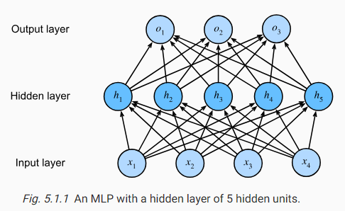
This MLP has 4 inputs, 3 outputs, and its hidden layer contains 5 hidden units. Since the input layer does not involve any calculations, producing outputs with this network requires implementing the computations for both the hidden and output layers; thus, the number of layers in this MLP is 2. Note that both layers are fully connected. Every input influences every neuron in the hidden layer, and each of these in turn influences every neuron in the output layer. Alas, we are not quite done yet.
이 MLP에는 4개의 입력과 3개의 출력이 있으며 숨겨진 레이어에는 5개의 숨겨진 유닛이 포함되어 있습니다. 입력 레이어에는 계산이 포함되지 않으므로 이 네트워크로 출력을 생성하려면 숨겨진 레이어와 출력 레이어 모두에 대한 계산을 구현해야 합니다. 따라서 이 MLP의 레이어 수는 2입니다. 두 레이어가 완전히 연결되어 있음에 유의하십시오. 모든 입력은 숨겨진 레이어의 모든 뉴런에 영향을 미치고 이들 각각은 차례로 출력 레이어의 모든 뉴런에 영향을 줍니다. 아아, 아직 끝나지 않았습니다.
Affine function이란?
An affine function is a mathematical function that represents a linear transformation of variables, followed by a translation. It has the general form:
어파인 함수는 변수의 선형 변환과 이동(translation)을 함께 나타내는 수학적인 함수입니다. 일반적인 형태는 다음과 같습니다:
f(x) = Ax + b
In this equation, A is a matrix representing the linear transformation, x is the input vector, and b is a vector representing the translation. The affine function maps the input vector x to a new vector by applying the linear transformation and then adding the translation.
이 식에서 A는 선형 변환을 나타내는 행렬이고, x는 입력 벡터이며, b는 이동 벡터입니다. 어파인 함수는 입력 벡터 x를 새로운 벡터로 변환하기 위해 선형 변환을 적용한 다음 이동을 추가합니다.
An affine function combines a linear transformation and a translation. It takes an input vector, applies a linear transformation to it, and then adds a translation vector. This type of function is widely used in mathematics, computer graphics, and machine learning for tasks such as geometric transformations, regression analysis, and neural networks.
어파인 함수는 선형 변환과 이동을 결합한 형태로, 수학, 컴퓨터 그래픽스, 기계 학습 등에서 기하학적 변환, 회귀 분석, 신경망 등 다양한 작업에 널리 사용됩니다.
5.1.1.3. From Linear to Nonlinear
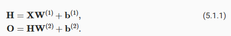
As before, we denote by the matrix X∈Rn×d a minibatch of n examples where each example has h inputs (features). For a one-hidden-layer MLP whose hidden layer has ℎ hidden units, we denote by H∈Rn×ℎ the outputs of the hidden layer, which are hidden representations. Since the hidden and output layers are both fully connected, we have hidden-layer weights W(1)∈Rd×ℎ and biases b(1)∈R1×ℎ and output-layer weights W(2)∈Rℎ×q and biases b(2)∈R1×q. This allows us to calculate the outputs O∈R1×a of the one-hidden-layer MLP as follows:
이전과 마찬가지로 각 예제에 h개의 inputs (features)이 있는 n examples 의 미니 배치를 행렬 X∈Rn×d로 표시합니다. hidden layer에 ℎ개의 hidden units가 있는 one-hidden-layer MLP의 경우 hidden layer의 출력을 H∈Rn×ℎ로 표시합니다. 이는 hidden representations입니다. 숨겨진 레이어와 출력 레이어가 모두 완전히 연결되어 있으므로 숨겨진 레이어 가중치 W(1)∈Rd×ℎ 및 Bias b(1)∈R1×ℎ 및 출력 레이어 가중치 W(2)∈Rℎ×q 및 편향 b(2)∈R1×q. 이를 통해 다음과 같이 하나의 숨겨진 레이어 MLP의 출력 O∈R1×a를 계산할 수 있습니다.
Note that after adding the hidden layer, our model now requires us to track and update additional sets of parameters. So what have we gained in exchange? You might be surprised to find out that—in the model defined above—we gain nothing for our troubles! The reason is plain. The hidden units above are given by an affine function of the inputs, and the outputs (pre-softmax) are just an affine function of the hidden units. An affine function of an affine function is itself an affine function. Moreover, our linear model was already capable of representing any affine function.
은닉층(hidden layer)를 추가한 후 모델은 이제 추가 매개변수 세트를 추적하고 업데이트해야 합니다. 그래서 우리는 그 대가로 무엇을 얻었습니까? 위에 정의된 모델에서 우리는 문제를 겪으면서 얻는 것이 없다는 사실에 놀랄 수도 있습니다! 이유는 간단합니다. 위의 은닉 유닛은 입력의 아핀 함수에 의해 주어지며 출력(pre-softmax)은 은닉 유닛의 아핀 함수일 뿐입니다. 아핀 함수의 아핀 함수는 그 자체가 아핀 함수이다. 게다가, 우리의 선형 모델은 이미 모든 아핀 함수를 나타낼 수 있었습니다.
To see this formally we can just collapse out the hidden layer in the above definition, yielding an equivalent single-layer model with parameters W=W(1)W(2) and b=b(1)W(2)+b(2):
이를 공식적으로 확인하기 위해 위 정의에서 숨겨진 레이어를 축소하여 매개변수 W=W(1)W(2) 및 b=b(1)W(2)+b( 2)를 갖는 등가 단일 레이어 모델을 생성합니다 :

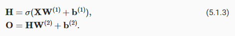
In order to realize the potential of multilayer architectures, we need one more key ingredient: a nonlinear activation function σ to be applied to each hidden unit following the affine transformation. For instance, a popular choice is the ReLU (Rectified Linear Unit) activation function (Nair and Hinton, 2010) σ(x)=max(0,x) operating on its arguments element-wise. The outputs of activation functions σ(⋅) are called activations. In general, with activation functions in place, it is no longer possible to collapse our MLP into a linear model:
다층 아키텍처의 잠재력을 실현하려면 비선형 활성화 함수 σ와 같은 핵심 요소가 하나 더 필요합니다. 아핀 변환 후 각 히든 유닛에 적용됩니다. 예를 들어, 널리 사용되는 선택은 ReLU(Rectified Linear Unit) 활성화 함수(Nair and Hinton, 2010) σ(x)=max(0,x) 인수에서 요소별로 작동하는 것입니다. 활성화 함수 σ(⋅)의 출력을 활성화라고 합니다. 일반적으로 활성화 기능이 있으면 더 이상 MLP를 선형 모델로 축소할 수 없습니다.
Since each row in X corresponds to an example in the minibatch, with some abuse of notation, we define the nonlinearity σ to apply to its inputs in a row-wise fashion, i.e., one example at a time. Note that we used the same notation for softmax when we denoted a row-wise operation in Section 4.1.1.3. Quite frequently the activation functions we use apply not merely row-wise but element-wise. That means that after computing the linear portion of the layer, we can calculate each activation without looking at the values taken by the other hidden units.
X의 각 행은 표기법을 남용하여 미니 배치의 예에 해당하므로 비선형성 σ를 정의하여 행 방향 방식으로(즉, 한 번에 하나의 예) 입력에 적용합니다. 섹션 4.1.1.3에서 행 방식 연산을 표시할 때 softmax에 대해 동일한 표기법을 사용했음에 유의하십시오. 꽤 자주 우리가 사용하는 활성화 함수는 단순히 행 단위가 아니라 요소 단위로 적용됩니다. 즉, 레이어의 선형 부분을 계산한 후 다른 히든 유닛에서 가져온 값을 보지 않고 각 활성화를 계산할 수 있습니다.
To build more general MLPs, we can continue stacking such hidden layers, e.g., H(1)=σ1(XW(1)+b(1)) and H(2)=σ2(H(1)W(2)+b(2)), one atop another, yielding ever more expressive models.
보다 일반적인 MLP들을 build 하기 위해 우리는 그런 hidden layer들을 계속 쌓아 갈 수 있습니다.

하나 위에 다른 하나를 쌓는 식으로 좀 더 모델들을 풍성하게 만들 수 있습니다.
5.1.1.4. Universal Approximators
We know that the brain is capable of very sophisticated statistical analysis. As such, it is worth asking, just how powerful a deep network could be. This question has been answered multiple times, e.g., in Cybenko (1989) in the context of MLPs, and in Micchelli (1984) in the context of reproducing kernel Hilbert spaces in a way that could be seen as radial basis function (RBF) networks with a single hidden layer. These (and related results) suggest that even with a single-hidden-layer network, given enough nodes (possibly absurdly many), and the right set of weights, we can model any function. Actually learning that function is the hard part, though. You might think of your neural network as being a bit like the C programming language. The language, like any other modern language, is capable of expressing any computable program. But actually coming up with a program that meets your specifications is the hard part.
우리는 뇌가 매우 정교한 통계 분석이 가능하다는 것을 알고 있습니다. 따라서 딥 네트워크가 얼마나 강력할 수 있는지 물어볼 가치가 있습니다. 이 질문은 예를 들어 MLP의 맥락에서 Cybenko(1989)와 방사형 기저 함수(RBF) 네트워크로 볼 수 있는 방식으로 커널 Hilbert 공간을 재생산하는 맥락에서 Micchelli(1984)에서 하나의 은닉층으로 여러 번 답변되었습니다. 이들(및 관련 결과)은 단일 은닉층 네트워크에서도 충분한 노드(어쩌면 터무니없이 많을 수 있음)와 올바른 가중치 세트가 주어지면 모든 기능을 모델링할 수 있음을 시사합니다. 하지만 실제로 그 기능을 배우는 것은 어려운 부분입니다. 신경망이 C 프로그래밍 언어와 비슷하다고 생각할 수 있습니다. 이 언어는 다른 현대 언어와 마찬가지로 계산 가능한 모든 프로그램을 표현할 수 있습니다. 그러나 실제로 귀하의 사양에 맞는 프로그램을 생각해내는 것은 어려운 부분입니다.
Moreover, just because a single-hidden-layer network can learn any function does not mean that you should try to solve all of your problems with single-hidden-layer networks. In fact, in this case kernel methods are way more effective, since they are capable of solving the problem exactly even in infinite dimensional spaces (Kimeldorf and Wahba, 1971, Schölkopf et al., 2001). In fact, we can approximate many functions much more compactly by using deeper (vs. wider) networks (Simonyan and Zisserman, 2014). We will touch upon more rigorous arguments in subsequent chapters.
또한 단일 은닉층 네트워크가 모든 기능을 학습할 수 있다고 해서 모든 문제를 단일 은닉층 네트워크로 해결해야 한다는 의미는 아닙니다. 실제로 이 경우 커널 방법은 무한 차원 공간에서도 문제를 정확하게 해결할 수 있기 때문에 훨씬 더 효과적입니다(Kimeldorf and Wahba, 1971, Schölkopf et al., 2001). 실제로 우리는 더 깊은(더 넓은) 네트워크를 사용하여 훨씬 더 간결하게 많은 함수를 근사화할 수 있습니다(Simonyan and Zisserman, 2014). 다음 장에서 더 엄격한 주장을 다룰 것입니다.
5.1.2. Activation Functions
Activation functions decide whether a neuron should be activated or not by calculating the weighted sum and further adding bias with it. They are differentiable operators to transform input signals to outputs, while most of them add non-linearity. Because activation functions are fundamental to deep learning, let’s briefly survey some common activation functions.
활성화 함수는 가중 합을 계산하고 바이어스를 추가하여 뉴런을 활성화해야 하는지 여부를 결정합니다. 입력 신호를 출력으로 변환하는 미분 연산자이며 대부분 비선형성을 추가합니다. 활성화 함수는 딥 러닝의 기본이기 때문에 몇 가지 일반적인 활성화 함수를 간략하게 살펴보겠습니다.
Activation Function이란?
Activation functions are mathematical functions that introduce non-linearity to neural networks. They are applied to the outputs of individual neurons in a neural network to determine their activation state. Activation functions play a crucial role in neural networks as they introduce non-linear transformations, allowing the network to model complex relationships between inputs and outputs.
활성화 함수(Activation functions)는 신경망에서 개별 뉴런의 출력에 적용되는 수학적인 함수로, 신경망에 비선형성(non-linearity)을 도입합니다. 이 함수들은 신경망의 개별 뉴런의 활성화 상태를 결정하는 데 사용됩니다. 활성화 함수는 신경망에서 중요한 역할을 하며, 비선형 변환을 도입하여 입력과 출력 간의 복잡한 관계를 모델링할 수 있게 합니다.
Activation functions help neural networks learn and make predictions by mapping the input values to a desired output range. They introduce non-linearities, allowing the network to approximate any continuous function. Without activation functions, the neural network would simply be a linear transformation, unable to learn complex patterns and relationships in the data.
활성화 함수는 입력 값을 원하는 출력 범위로 매핑하여 신경망이 학습하고 예측하는 데 도움을 줍니다. 비선형성을 도입하여 신경망은 연속 함수를 근사화할 수 있게 됩니다. 활성화 함수가 없다면 신경망은 단순히 선형 변환만 수행하는 것이 되어 복잡한 패턴과 관계를 학습할 수 없게 됩니다.
Commonly used activation functions include sigmoid, tanh, ReLU (Rectified Linear Unit), and softmax. Each activation function has its own characteristics and is suitable for different scenarios. The choice of activation function depends on the problem at hand, network architecture, and desired properties such as non-linearity, differentiability, and output range.
일반적으로 사용되는 활성화 함수에는 시그모이드(Sigmoid), 하이퍼볼릭 탄젠트(Tanh), ReLU(렉티파이드 선형 유닛), 소프트맥스(Softmax) 등이 있습니다. 각 활성화 함수는 고유한 특성을 가지며, 다른 상황에 적합합니다. 활성화 함수의 선택은 주어진 문제, 신경망 구조 및 비선형성, 미분 가능성, 출력 범위 등 원하는 속성에 따라 달라집니다.
By applying activation functions, neural networks can model complex functions and capture intricate patterns in data, enabling them to solve a wide range of tasks including classification, regression, and generative modeling.
활성화 함수를 적용함으로써 신경망은 복잡한 함수를 모델링하고 데이터의 복잡한 패턴을 포착할 수 있으며, 이를 통해 분류, 회귀, 생성 모델링 등 다양한 작업을 해결할 수 있습니다.
5.1.2.1. ReLU Function
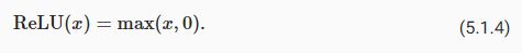
The most popular choice, due to both simplicity of implementation and its good performance on a variety of predictive tasks, is the rectified linear unit (ReLU) (Nair and Hinton, 2010). ReLU(Rectified linear Unit) provides a very simple nonlinear transformation. Given an element x, the function is defined as the maximum of that element and 0:
구현의 단순성과 다양한 예측 작업에 대한 우수한 성능으로 인해 가장 인기 있는 선택은 정류 선형 장치(ReLU)입니다(Nair 및 Hinton, 2010). ReLU는 매우 간단한 비선형 변환을 제공합니다. 요소 x가 주어지면 함수는 해당 요소의 최대값과 0으로 정의됩니다.
ReLU Function 이란?
The Rectified Linear Unit (ReLU) function is an activation function commonly used in neural networks. It is defined as f(x) = max(0, x), where x is the input to the function. In other words, if the input is positive, ReLU returns the input value itself, and if the input is negative, ReLU returns zero.
활성화 함수인 ReLU(Rectified Linear Unit) 함수는 신경망에서 흔히 사용되는 활성화 함수입니다. 이 함수는 f(x) = max(0, x)로 정의되며, 여기서 x는 함수의 입력입니다. 다시 말해, 입력이 양수인 경우 ReLU는 입력 값을 그대로 반환하고, 입력이 음수인 경우 ReLU는 0을 반환합니다.
ReLU is popular in deep learning because it introduces non-linearity to the network and helps address the vanishing gradient problem. It allows the network to learn complex patterns and make the learning process more efficient. ReLU is computationally efficient and easy to implement, which contributes to its widespread usage.
ReLU는 딥러닝에서 인기가 있으며, 네트워크에 비선형성을 도입하고 기울기 소실 문제(vanishing gradient problem)를 해결하는 데 도움이 됩니다. 이를 통해 네트워크가 복잡한 패턴을 학습하고 학습 과정을 효율적으로 만들 수 있습니다. ReLU는 계산적으로 효율적이고 구현하기 쉬운 특징을 가지고 있어 널리 사용되고 있습니다.
The key advantage of ReLU is that it does not saturate for positive inputs, unlike other activation functions such as sigmoid or hyperbolic tangent. This means that ReLU does not suffer from the vanishing gradient problem when dealing with large positive inputs. However, one limitation of ReLU is that it can cause dead neurons, where neurons that output zero become inactive and stop learning. This issue can be mitigated by using variants of ReLU, such as Leaky ReLU or Parametric ReLU, which address the dead neuron problem.
ReLU의 주요 장점은 양수 입력에 대해서 saturate(포화, 처리)되지 않는다는 점입니다. 시그모이드 또는 하이퍼볼릭 탄젠트와 같은 다른 활성화 함수와는 달리, 큰 양수 입력과 관련하여 기울기 소실 문제가 발생하지 않습니다. 그러나 ReLU의 한 가지 제한은 꺼진 뉴런(dead neurons)을 일으킬 수 있다는 점입니다. 출력이 0이 되는 뉴런은 비활성화되어 학습을 멈추는 문제가 발생할 수 있습니다. 이 문제는 Leaky ReLU 또는 Parametric ReLU와 같은 ReLU의 변형을 사용하여 완화할 수 있습니다.
ReLU is primarily used in the hidden layers of neural networks, while other activation functions like softmax or sigmoid are commonly used in the output layer for specific tasks such as classification or probability estimation.
ReLU는 주로 신경망의 은닉층에서 사용되며, 분류 또는 확률 추정과 같은 특정 작업을 위해 softmax 또는 시그모이드와 같은 다른 활성화 함수가 출력층에서 사용됩니다.
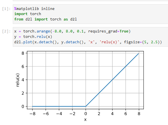
Informally, the ReLU function retains only positive elements and discards all negative elements by setting the corresponding activations to 0. To gain some intuition, we can plot the function. As you can see, the activation function is piecewise linear.
비공식적으로 ReLU 함수는 해당 활성화를 0으로 설정하여 양수 요소만 유지하고 음수 요소를 모두 버립니다. 직관력을 얻기 위해 함수를 플로팅(plot )할 수 있습니다. 보시다시피 활성화 함수는 구분 선형입니다.
x = torch.arange(-8.0, 8.0, 0.1, requires_grad=True)
y = torch.relu(x)
d2l.plot(x.detach(), y.detach(), 'x', 'relu(x)', figsize=(5, 2.5))
위 코드는 ReLU 함수의 입력 범위에 따른 출력을 시각화하는 내용입니다. 코드의 각 줄을 설명하면 다음과 같습니다:
- -8.0부터 8.0까지 0.1 간격으로 숫자를 생성합니다. 이 숫자는 ReLU 함수의 입력값으로 사용됩니다. requires_grad=True는 이 변수에 대한 기울기(gradient)를 계산할 필요가 있다는 것을 나타냅니다.
- 입력값 x를 ReLU 함수에 적용하여 출력값 y를 계산합니다. ReLU 함수는 입력값이 양수인 경우에는 그대로 반환하고, 음수인 경우에는 0으로 변환합니다.
- d2l.plot 함수를 사용하여 입력값 x와 출력값 y를 시각화합니다. x축은 x의 값들을 나타내고, y축은 y의 값들을 나타냅니다. 그래프의 제목은 'relu(x)'이며, figsize=(5, 2.5)는 그래프의 크기를 지정합니다.
이 코드를 실행하면 입력값 x에 대한 ReLU 함수의 출력값이 그래프로 나타나게 됩니다. 입력값이 양수인 경우에는 입력값과 같은 값을 출력하며, 음수인 경우에는 0을 출력합니다. 이를 통해 ReLU 함수의 특징을 시각적으로 확인할 수 있습니다.
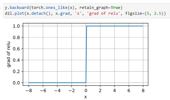
When the input is negative, the derivative of the ReLU function is 0, and when the input is positive, the derivative of the ReLU function is 1. Note that the ReLU function is not differentiable when the input takes value precisely equal to 0. In these cases, we default to the left-hand-side derivative and say that the derivative is 0 when the input is 0. We can get away with this because the input may never actually be zero (mathematicians would say that it is nondifferentiable on a set of measure zero). There is an old adage that if subtle boundary conditions matter, we are probably doing (real) mathematics, not engineering. That conventional wisdom may apply here, or at least, the fact that we are not performing constrained optimization (Mangasarian, 1965, Rockafellar, 1970). We plot the derivative of the ReLU function plotted below.
입력이 음수이면 ReLU 함수의 도함수는 0이고 입력이 양수이면 ReLU 함수의 도함수는 1입니다. ReLU 함수는 입력 값이 정확하게 0일 때 미분할 수 없습니다. 이러한 경우, 기본적으로 왼쪽 도함수를 사용하고 입력이 0일 때 도함수가 0이라고 말합니다. 입력이 실제로 0이 될 수 없기 때문에 이를 무시할 수 있습니다. 제로 측정 세트). 미묘한 경계 조건이 중요하다면 공학이 아니라 (진짜) 수학을 하고 있을 것이라는 오래된 속담이 있습니다. 이러한 통념은 여기에 적용될 수 있으며, 적어도 우리가 제한된 최적화를 수행하지 않는다는 사실이 적용될 수 있습니다(Mangasarian, 1965, Rockafellar, 1970). 아래에 그려진 ReLU 함수의 도함수를 그립니다.
y.backward(torch.ones_like(x), retain_graph=True)
d2l.plot(x.detach(), x.grad, 'x', 'grad of relu', figsize=(5, 2.5))
위 코드는 ReLU 함수의 역전파 과정에서의 기울기(gradient)를 시각화하는 내용입니다. 코드의 각 줄을 한글로 설명하면 다음과 같습니다:
- y.backward(torch.ones_like(x), retain_graph=True)는 y를 x에 대해 역전파하면서 기울기를 계산합니다. torch.ones_like(x)는 x와 동일한 shape를 가지며 모든 원소가 1인 텐서입니다. retain_graph=True는 그래프의 계산 그래프를 유지하여 여러 번의 역전파를 수행할 수 있도록 합니다.
- d2l.plot 함수를 사용하여 입력값 x와 해당하는 기울기 x.grad를 시각화합니다. x축은 x의 값들을 나타내고, y축은 x의 기울기 값을 나타냅니다. 그래프의 제목은 'grad of relu'이며, figsize=(5, 2.5)는 그래프의 크기를 지정합니다.
이 코드를 실행하면 입력값 x에 대한 ReLU 함수의 역전파 과정에서의 기울기가 그래프로 나타나게 됩니다. 입력값이 양수인 경우에는 기울기가 1로 유지되며, 음수인 경우에는 기울기가 0이 됩니다. ReLU 함수의 역전파 과정에서 음수 입력값에 대한 기울기가 0이 되는 특징을 시각적으로 확인할 수 있습니다.
The reason for using ReLU is that its derivatives are particularly well behaved: either they vanish or they just let the argument through. This makes optimization better behaved and it mitigated the well-documented problem of vanishing gradients that plagued previous versions of neural networks (more on this later).
ReLU를 사용하는 이유는 그 파생물이 특히 잘 작동하기 때문입니다. 사라지거나 인수를 그냥 통과시킵니다. 이를 통해 최적화가 더 잘 작동하고 이전 버전의 신경망을 괴롭혔던 잘 알려진 기울기 소실 문제를 완화했습니다(자세한 내용은 나중에 설명).
Note that there are many variants to the ReLU function, including the parameterized ReLU (pReLU) function (He et al., 2015). This variation adds a linear term to ReLU, so some information still gets through, even when the argument is negative:
매개변수화된(parameterized ) ReLU(pReLU) 함수를 포함하여 ReLU 함수에는 많은 변형이 있습니다(He et al., 2015). 이 변형은 ReLU에 선형 항을 추가하므로 인수가 음수인 경우에도 일부 정보가 계속 전달됩니다.

5.1.2.2. Sigmoid Function
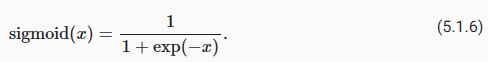
The sigmoid function transforms its inputs, for which values lie in the domain R, to outputs that lie on the interval (0, 1). For that reason, the sigmoid is often called a squashing function: it squashes any input in the range (-inf, inf) to some value in the range (0, 1):
시그모이드 함수는 값이 도메인 R에 있는 입력을 구간 (0, 1)에 있는 출력으로 변환합니다. 이러한 이유로 시그모이드는 종종 스쿼싱 함수라고 합니다. (-inf, inf) 범위의 모든 입력을 (0, 1) 범위의 일부 값으로 스쿼시합니다.
Sigmoid Functions란?
The Sigmoid function, also known as the logistic function, is a commonly used activation function in neural networks. It maps the input value to a range between 0 and 1. The mathematical expression for the Sigmoid function is:
시그모이드 함수 또는 로지스틱 함수는 신경망에서 널리 사용되는 활성화 함수입니다. 이 함수는 입력 값을 0과 1 사이의 범위로 매핑합니다. 수학적으로는 다음과 같이 표현됩니다:
f(x) = 1 / (1 + exp(-x))
In neural networks, the Sigmoid function is often used to introduce non-linearity in the model. It is particularly useful in models where the output needs to be interpreted as a probability or where the output range needs to be constrained between 0 and 1.
신경망에서 시그모이드 함수는 모델에 비선형성을 도입하는 데 유용합니다. 출력을 확률로 해석해야 하는 모델이나 출력 범위를 0과 1 사이로 제한해야 하는 경우에 특히 유용합니다.
When the input to the Sigmoid function is large, the output tends to 1, and when the input is small, the output tends to 0. The Sigmoid function has a smooth and continuous shape, which makes it differentiable, enabling efficient computation of gradients during backpropagation.
시그모이드 함수의 입력이 큰 경우 출력은 1에 가까워지고, 입력이 작은 경우 출력은 0에 가까워집니다. 시그모이드 함수는 부드럽고 연속적인 형태를 가지며, 이는 미분 가능성을 제공하여 역전파(backpropagation) 과정에서 그레이디언트를 효율적으로 계산할 수 있게 합니다.
The Sigmoid function is widely used in tasks such as binary classification, where the goal is to classify data into two classes. It is also used in certain types of recurrent neural networks (RNNs) and in the output layer of multi-class classification models.
시그모이드 함수는 이진 분류와 같은 작업에서 널리 사용됩니다. 여기서 목표는 데이터를 두 개의 클래스로 분류하는 것입니다. 또한 특정 유형의 순환 신경망(RNN)이나 다중 클래스 분류 모델의 출력층에서도 사용됩니다.
Overall, the Sigmoid function allows neural networks to model non-linear relationships and make predictions within a bounded range of values, which makes it a valuable tool in many machine learning applications.
시그모이드 함수는 신경망이 비선형 관계를 모델링하고, 한정된 값 범위 내에서 예측을 수행할 수 있도록 합니다. 따라서 다양한 기계 학습 응용 분야에서 가치 있는 도구로 사용됩니다.
In the earliest neural networks, scientists were interested in modeling biological neurons which either fire or do not fire. Thus the pioneers of this field, going all the way back to McCulloch and Pitts, the inventors of the artificial neuron, focused on thresholding units (McCulloch and Pitts, 1943). A thresholding activation takes value 0 when its input is below some threshold and value 1 when the input exceeds the threshold.
초기 신경망에서 과학자들은 발화하거나 발화하지 않는 생물학적 뉴런을 모델링하는 데 관심이 있었습니다. 따라서 이 분야의 개척자들은 인공 뉴런의 발명가인 McCulloch와 Pitts까지 거슬러 올라가 thresholding units(임계값 단위)에 초점을 맞췄습니다(McCulloch and Pitts, 1943). 임계값 활성화는 입력이 임계값 미만일 때 값 0을 취하고 입력이 임계값을 초과할 때 값 1을 갖습니다.
When attention shifted to gradient based learning, the sigmoid function was a natural choice because it is a smooth, differentiable approximation to a thresholding unit. Sigmoids are still widely used as activation functions on the output units, when we want to interpret the outputs as probabilities for binary classification problems: you can think of the sigmoid as a special case of the softmax. However, the sigmoid has mostly been replaced by the simpler and more easily trainable ReLU for most use in hidden layers. Much of this has to do with the fact that the sigmoid poses challenges for optimization (LeCun et al., 1998) since its gradient vanishes for large positive and negative arguments. This can lead to plateaus that are difficult to escape from. Nonetheless sigmoids are important. In later chapters (e.g., Section 10.1) on recurrent neural networks, we will describe architectures that leverage sigmoid units to control the flow of information across time.
10.1. Long Short-Term Memory (LSTM) — Dive into Deep Learning 1.0.0-beta0 documentation
d2l.ai
관심이 그래디언트 기반 학습으로 옮겨갔을 때 시그모이드 함수는 임계값 단위에 대한 매끄럽고 미분 가능한 근사이기 때문에 자연스러운 선택이었습니다. 시그모이드는 이진 분류 문제에 대한 확률로 출력을 해석하려는 경우 출력 단위의 활성화 함수로 여전히 널리 사용됩니다. 시그모이드는 소프트맥스의 특수한 경우로 생각할 수 있습니다. 그러나 시그모이드는 은닉층에서 대부분 사용하기 위해 더 간단하고 쉽게 훈련할 수 있는 ReLU로 대체되었습니다. 이것의 많은 부분은 sigmoid가 최적화에 대한 문제를 제기한다는 사실과 관련이 있습니다(LeCun et al., 1998). 큰 양의 인수와 음의 인수에 대해 기울기가 사라지기 때문입니다. 이것은 탈출하기 어려운 고원으로 이어질 수 있습니다. 그럼에도 불구하고 시그모이드는 중요합니다. 순환 신경망에 대한 이후 장(예: 섹션 10.1)에서는 시그모이드 단위를 활용하여 시간에 따른 정보 흐름을 제어하는 아키텍처를 설명합니다.
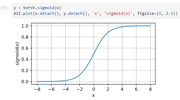
Below, we plot the sigmoid function. Note that when the input is close to 0, the sigmoid function approaches a linear transformation.
아래에서 시그모이드 함수를 플로팅합니다. 입력이 0에 가까울 때 시그모이드 함수는 선형 변환에 접근합니다.
y = torch.sigmoid(x)
d2l.plot(x.detach(), y.detach(), 'x', 'sigmoid(x)', figsize=(5, 2.5))
해당 코드는 시그모이드 함수를 사용하여 입력값에 대한 출력값을 계산하고 그래프로 나타내는 역할을 합니다. 코드를 한 줄씩 설명하겠습니다.
- y = torch.sigmoid(x): 입력 x에 대해 시그모이드 함수를 적용하여 출력 y를 계산합니다. 시그모이드 함수는 torch.sigmoid 함수를 사용하여 구현됩니다.
- d2l.plot(x.detach(), y.detach(), 'x', 'sigmoid(x)', figsize=(5, 2.5)): 계산된 입력 x와 해당 입력에 대한 출력 y를 그래프로 표시합니다. d2l.plot 함수는 입력 데이터와 축 레이블, 그리고 그래프의 크기 등을 인자로 받아 그래프를 생성합니다.
이 코드는 입력 x를 시그모이드 함수에 적용하여 얻은 출력 y를 그래프로 시각화하는 것입니다. 시그모이드 함수의 특성을 살펴볼 수 있으며, 입력이 양수인 경우 출력은 0에 가까워지고, 입력이 음수인 경우 출력은 1에 가까워집니다.
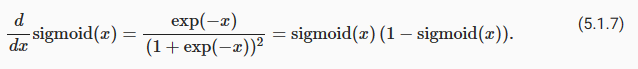
The derivative of the sigmoid function is given by the following equation:
시그모이드 함수의 도함수(derivative )는 다음 방정식(equation)으로 제공됩니다.
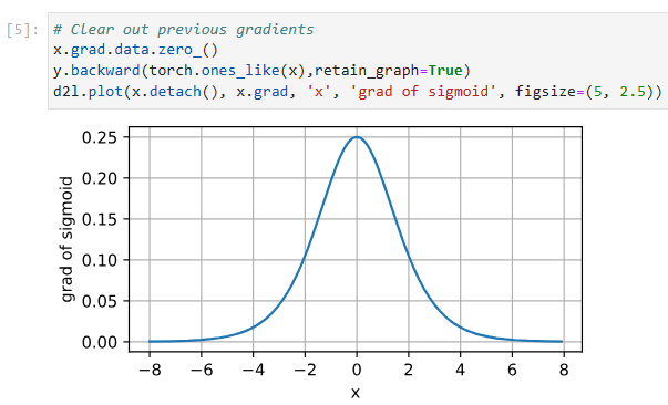
The derivative of the sigmoid function is plotted below. Note that when the input is 0, the derivative of the sigmoid function reaches a maximum of 0.25. As the input diverges from 0 in either direction, the derivative approaches 0.
시그모이드 함수의 도함수(derivative )는 다음과 같습니다. 입력이 0일 때 시그모이드 함수의 도함수는 최대 0.25에 도달합니다. 입력이 0에서 어느 방향으로든 갈라지면 도함수는 0에 접근합니다.
# Clear out previous gradients
x.grad.data.zero_()
y.backward(torch.ones_like(x),retain_graph=True)
d2l.plot(x.detach(), x.grad, 'x', 'grad of sigmoid', figsize=(5, 2.5))
위 코드는 시그모이드 함수의 그래디언트를 계산하고, 그래프로 나타내는 역할을 합니다. 코드를 한 줄씩 설명하겠습니다.
- x.grad.data.zero_(): 이전의 그래디언트 값을 초기화합니다. x의 그래디언트 값을 계산하기 전에 이전의 값들을 지워줍니다.
- y.backward(torch.ones_like(x),retain_graph=True): y를 x에 대해 역전파합니다. torch.ones_like(x)는 x와 동일한 크기의 모든 원소가 1인 텐서입니다. retain_graph=True는 그래디언트 계산 후 그래프를 유지하는 옵션입니다.
- d2l.plot(x.detach(), x.grad, 'x', 'grad of sigmoid', figsize=(5, 2.5)): x에 대한 그래디언트 값을 그래프로 표시합니다. x.detach()는 x의 값만을 가져오고 그래디언트 계산을 끊는 역할을 합니다. 그래프는 입력 데이터 x와 그래디언트 값을 x축과 y축으로 나타내며, 그래디언트의 변화를 시각화합니다.
이 코드는 시그모이드 함수를 역전파하여 그래디언트 값을 계산하고, 그래프로 시각화하는 역할을 합니다. 시그모이드 함수의 그래디언트는 입력 값에 따라 양수 또는 음수로 변화합니다. 그래프를 통해 시그모이드 함수의 그래디언트의 특성을 살펴볼 수 있습니다.
5.1.2.3. Tanh Function
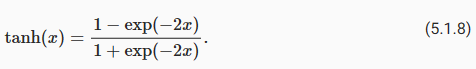
Like the sigmoid function, the tanh (hyperbolic tangent) function also squashes its inputs, transforming them into elements on the interval between -1 and 1:
시그모이드 함수와 마찬가지로 tanh(하이퍼볼릭 탄젠트) 함수도 입력을 스쿼시하여 -1과 1 사이의 간격에 있는 요소로 변환합니다.
Tanh Function 이란?
The hyperbolic tangent function, commonly referred to as the "tanh" function, is a mathematical function that maps real-valued numbers to the range of [-1, 1]. It is defined as follows:
하이퍼볼릭 탄젠트 함수, 일반적으로 "tanh" 함수라고 불리는 함수는 실수 값을 [-1, 1] 범위로 매핑하는 수학 함수입니다. 다음과 같이 정의됩니다:
tanh(x) = (e^x - e^(-x)) / (e^x + e^(-x))
The tanh function has an "S"-shaped curve and is symmetric around the origin. It is widely used as an activation function in neural networks. Similar to the sigmoid function, the tanh function is also nonlinear and continuously differentiable.
tanh 함수는 "S" 모양의 곡선을 가지며 원점을 중심으로 대칭적입니다. 신경망에서 활성화 함수로 널리 사용됩니다. Sigmoid 함수와 마찬가지로 tanh 함수도 비선형이며 연속적으로 미분 가능합니다.
The tanh function has several properties that make it useful in machine learning tasks. It squashes input values to the range of [-1, 1], which can help in controlling the gradient flow during the backpropagation process. It also produces zero-centered outputs, which can be beneficial for learning in certain scenarios.
tanh 함수는 기계 학습 작업에서 유용한 속성을 갖고 있습니다. 입력 값을 [-1, 1] 범위로 압축하여 역전파 과정에서 그래디언트 흐름을 제어하는 데 도움이 될 수 있습니다. 또한 0을 중심으로 하는 출력 값을 생성하여 특정 시나리오에서의 학습에 유용합니다.
In summary, the tanh function is a nonlinear activation function that maps input values to the range of [-1, 1]. It is commonly used in neural networks for its desirable properties and ability to model complex relationships between inputs and outputs.
요약하면, tanh 함수는 입력 값을 [-1, 1] 범위로 매핑하는 비선형 활성화 함수입니다. 복잡한 관계를 모델링하는 데 유용한 속성과 능력을 갖춘 신경망에서 자주 사용됩니다.
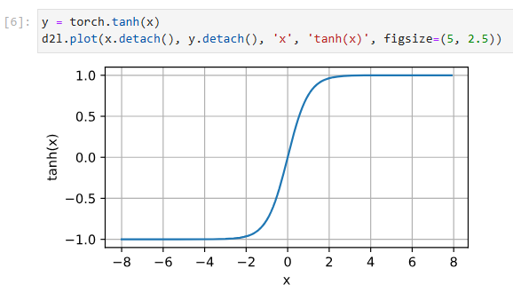
We plot the tanh function below. Note that as input nears 0, the tanh function approaches a linear transformation. Although the shape of the function is similar to that of the sigmoid function, the tanh function exhibits point symmetry about the origin of the coordinate system (Kalman and Kwasny, 1992).
아래에 tanh 함수를 플로팅합니다. 입력이 0에 가까워지면 tanh 함수는 선형 변환에 접근합니다. 함수의 모양은 시그모이드 함수와 유사하지만 tanh 함수는 좌표계의 원점을 중심으로 점대칭을 나타냅니다(Kalman and Kwasny, 1992).
y = torch.tanh(x)
d2l.plot(x.detach(), y.detach(), 'x', 'tanh(x)', figsize=(5, 2.5))
해당 코드는 하이퍼볼릭 탄젠트(tanh) 함수의 값을 계산하고, 그래프로 나타내는 역할을 합니다. 코드를 한 줄씩 설명하겠습니다.
- y = torch.tanh(x): x에 대한 하이퍼볼릭 탄젠트 함수의 값을 계산하여 y에 저장합니다. tanh 함수는 입력값을 -1과 1 사이의 값으로 압축하는 함수입니다.
- d2l.plot(x.detach(), y.detach(), 'x', 'tanh(x)', figsize=(5, 2.5)): x와 y 값을 그래프로 표시합니다. x.detach()와 y.detach()는 각각 x와 y의 값만을 가져온 후 그래프를 그리는 역할을 합니다. 그래프는 입력 데이터 x를 x축에, 하이퍼볼릭 탄젠트 함수의 결과값 y를 y축에 나타내며, 함수의 형태를 시각화합니다.
이 코드는 하이퍼볼릭 탄젠트 함수를 사용하여 입력 데이터 x에 대한 함수값을 계산하고, 그래프로 시각화하는 역할을 합니다. 하이퍼볼릭 탄젠트 함수는 입력값을 -1과 1 사이의 값으로 압축하므로, 그래프에서는 이러한 특성을 확인할 수 있습니다.
The derivative of the tanh function is:
tanh 함수의 도함수는 다음과 같습니다.
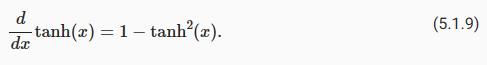
It is plotted below. As the input nears 0, the derivative of the tanh function approaches a maximum of 1. And as we saw with the sigmoid function, as input moves away from 0 in either direction, the derivative of the tanh function approaches 0.
아래에 그려져 있습니다. 입력이 0에 가까워지면 tanh 함수의 도함수는 최대 1에 접근합니다. 그리고 시그모이드 함수에서 보았듯이 입력이 0에서 어느 방향으로든 멀어지면 tanh 함수의 도함수는 0에 접근합니다.
# Clear out previous gradients
x.grad.data.zero_()
y.backward(torch.ones_like(x),retain_graph=True)
d2l.plot(x.detach(), x.grad, 'x', 'grad of tanh', figsize=(5, 2.5))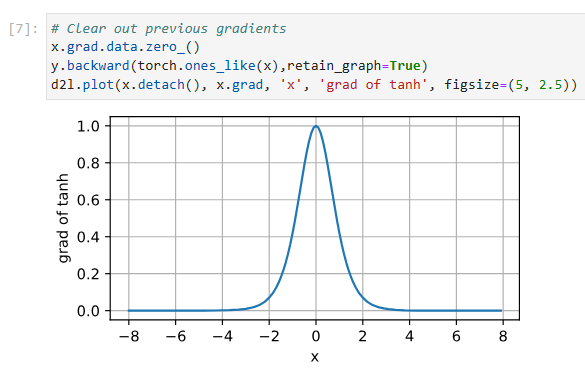
5.1.3. Summary and Discussion
We now know how to incorporate nonlinearities to build expressive multilayer neural network architectures. As a side note, your knowledge already puts you in command of a similar toolkit to a practitioner circa 1990. In some ways, you have an advantage over anyone working in the 1990s, because you can leverage powerful open-source deep learning frameworks to build models rapidly, using only a few lines of code. Previously, training these networks required researchers to code up layers and derivatives explicitly in C, Fortran, or even Lisp (in the case of LeNet).
우리는 이제 표현력이 풍부한 다층 신경망 아키텍처를 구축하기 위해 비선형성을 통합하는 방법을 알고 있습니다. 여담으로, 당신의 지식은 이미 당신을 1990년경 실무자와 유사한 툴킷을 지휘하게 했습니다. 어떤 면에서 당신은 강력한 오픈 소스 딥 러닝 프레임워크를 활용하여 몇 줄의 코드만 사용하여 신속하게 모델링합니다. 이전에는 이러한 네트워크를 교육하려면 연구자가 C, Fortran 또는 Lisp(LeNet의 경우)로 명시적으로 계층 및 파생 항목을 코딩해야 했습니다.
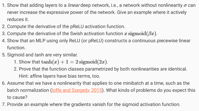
A secondary benefit is that ReLU is significantly more amenable to optimization than the sigmoid or the tanh function. One could argue that this was one of the key innovations that helped the resurgence of deep learning over the past decade. Note, though, that research in activation functions has not stopped. For instance, the GELU (Gaussian error linear unit) activation function xΦ(x) (Hendrycks and Gimpel, 2016), where Φ(x) is the standard Gaussian cumulative distribution function and the Swish activation function σ(x)=x sigmoid(βx) as proposed in Ramachandran et al. (2017) can yield better accuracy in many cases.
두 번째 이점은 ReLU가 시그모이드 또는 tanh 함수보다 훨씬 더 최적화하기 쉽다는 것입니다. 이것이 지난 10년 동안 딥 러닝의 부활을 도운 주요 혁신 중 하나라고 주장할 수 있습니다. 그러나 활성화 기능에 대한 연구는 중단되지 않았습니다. 예를 들어, GELU(Gaussian error linear unit) 활성화 함수 xΦ(x)(Hendrycks and Gimpel, 2016), 여기서 Φ(x)는 표준 가우스 누적 분포 함수이고 Swish 활성화 함수 σ(x)=x sigmoid( βx) Ramachandran et al. (2017)은 많은 경우에 더 나은 정확도를 얻을 수 있습니다.
5.1.4. Exercises
'Dive into Deep Learning > D2L Multilayer Perceptrons Builder Guide' 카테고리의 다른 글
| D2L - 5.7. Predicting House Prices on Kaggle (0) | 2023.07.03 |
|---|---|
| D2L - 5.6. Dropout (0) | 2023.07.03 |
| D2L - 5.5. Generalization in Deep Learning (0) | 2023.07.03 |
| D2L - 5.4. Numerical Stability and Initialization (0) | 2023.07.02 |
| D2L - 5.3. Forward Propagation, Backward Propagation, and Computational Graphs (0) | 2023.07.02 |
| D2L - 5.2. Implementation of Multilayer Perceptrons (0) | 2023.07.01 |
| D2L - 5. Multilayer Perceptrons (0) | 2023.06.30 |