

https://d2l.ai/chapter_recurrent-neural-networks/language-model.html
9.3. Language Models — Dive into Deep Learning 1.0.0-beta0 documentation
d2l.ai
9.3. Language Models
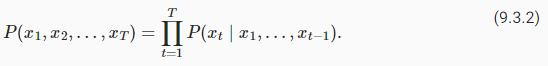
In Section 9.2, we see how to map text sequences into tokens, where these tokens can be viewed as a sequence of discrete observations, such as words or characters. Assume that the tokens in a text sequence of length T are in turn x1,x2,…,xT. The goal of language models is to estimate the joint probability of the whole sequence:
섹션 9.2에서는 텍스트 시퀀스를 토큰으로 매핑하는 방법을 살펴봅니다. 여기서 이러한 토큰은 단어나 문자와 같은 개별 관찰 시퀀스로 볼 수 있습니다. 길이가 T인 텍스트 시퀀스의 토큰이 차례로 x1,x2,…,xT라고 가정합니다. 언어 모델의 목표는 전체 시퀀스의 결합 확률을 추정하는 것입니다.

where statistical tools in Section 9.1 can be applied.
섹션 9.1의 통계 도구를 적용할 수 있습니다.
Language models are incredibly useful. For instance, an ideal language model would be able to generate natural text just on its own, simply by drawing one token at a time xt∼P(xt∣xt−1,…,x1). Quite unlike the monkey using a typewriter, all text emerging from such a model would pass as natural language, e.g., English text. Furthermore, it would be sufficient for generating a meaningful dialog, simply by conditioning the text on previous dialog fragments. Clearly we are still very far from designing such a system, since it would need to understand the text rather than just generate grammatically sensible content.
언어 모델은 매우 유용합니다. 예를 들어, 이상적인 언어 모델은 한 번에 하나의 토큰 xt∼P(xt∣xt−1,…,x1)을 그리는 것만으로 자체적으로 자연 텍스트를 생성할 수 있습니다. 타자기를 사용하는 원숭이와는 달리 이러한 모델에서 나오는 모든 텍스트는 자연어(예: 영어 텍스트)로 전달됩니다. 또한 이전 대화 조각에서 텍스트를 조건화하는 것만으로 의미 있는 대화를 생성하는 데 충분합니다. 분명히 우리는 그러한 시스템을 설계하는 것과는 거리가 멀다. 문법적으로 의미 있는 콘텐츠를 생성하는 것보다 텍스트를 이해해야 하기 때문이다.
Nonetheless, language models are of great service even in their limited form. For instance, the phrases “to recognize speech” and “to wreck a nice beach” sound very similar. This can cause ambiguity in speech recognition, which is easily resolved through a language model that rejects the second translation as outlandish. Likewise, in a document summarization algorithm it is worthwhile knowing that “dog bites man” is much more frequent than “man bites dog”, or that “I want to eat grandma” is a rather disturbing statement, whereas “I want to eat, grandma” is much more benign.
그럼에도 불구하고 언어 모델은 제한된 형식에서도 훌륭한 서비스를 제공합니다. 예를 들어, "to recognize speech"와 "to wreck a nice beach"라는 문구는 매우 비슷하게 들립니다. 이로 인해 음성 인식에서 모호성이 발생할 수 있으며, 두 번째 번역을 이상하다고 거부하는 언어 모델을 통해 쉽게 해결됩니다. 마찬가지로 문서 요약 알고리즘에서 "dog bites man"가 "man bites dog"보다 훨씬 더 자주 발생하거나 "I want to eat grandma"는 다소 불안한 진술인 반면 "I want to eat, grandma”가 훨씬 더 온화합니다.
import torch
from d2l import torch as d2l
9.3.1. Learning Language Models
The obvious question is how we should model a document, or even a sequence of tokens. Suppose that we tokenize text data at the word level. Let’s start by applying basic probability rules:
분명한 질문은 어떻게 문서 또는 일련의 토큰을 모델링하는가 하는겁니다. 단어 수준에서 텍스트 데이터를 토큰화한다고 가정합니다. 기본 확률 규칙을 적용하여 시작하겠습니다.
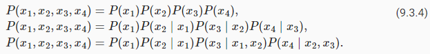
For example, the probability of a text sequence containing four words would be given as:
예를 들어, 4개의 단어를 포함하는 텍스트 시퀀스의 확률은 다음과 같이 주어집니다.

9.3.1.1. Markov Models and n-grams
Among those sequence model analysis in Section 9.1, let’s apply Markov models to language modeling. A distribution over sequences satisfies the Markov property of first order if P(xt+1∣xt,…,x1)=P(xt+1∣xt). Higher orders correspond to longer dependencies. This leads to a number of approximations that we could apply to model a sequence:
9.1절의 시퀀스 모델 분석 중 Markov 모델을 언어 모델링에 적용해 보자. 시퀀스에 대한 분포는 P(xt+1∣xt,…,x1)=P(xt+1∣xt)인 경우 1차 Markov 속성을 만족합니다. 더 높은 차수는 더 긴 종속성에 해당합니다. 이는 시퀀스를 모델링하는 데 적용할 수 있는 여러 가지 근사치로 이어집니다.
The probability formulae that involve one, two, and three variables are typically referred to as unigram, bigram, and trigram models, respectively. In order to compute the language model, we need to calculate the probability of words and the conditional probability of a word given the previous few words. Note that such probabilities are language model parameters.
1개, 2개 및 3개의 변수를 포함하는 확률 공식은 일반적으로 각각 유니그램, 바이그램 및 트라이그램 모델이라고 합니다. 언어 모델을 계산하기 위해서는 단어의 확률과 이전 몇 단어가 주어진 단어의 조건부 확률을 계산해야 합니다. 이러한 확률은 언어 모델 매개변수입니다.
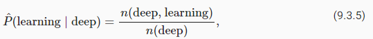
9.3.1.2. Word Frequency
Here, we assume that the training dataset is a large text corpus, such as all Wikipedia entries, Project Gutenberg, and all text posted on the Web. The probability of words can be calculated from the relative word frequency of a given word in the training dataset. For example, the estimate P^(deep) can be calculated as the probability of any sentence starting with the word “deep”. A slightly less accurate approach would be to count all occurrences of the word “deep” and divide it by the total number of words in the corpus. This works fairly well, particularly for frequent words. Moving on, we could attempt to estimate where n(x) and n(x,x′) are the number of occurrences of singletons and consecutive word pairs, respectively.
여기서는 교육 데이터 세트가 모든 Wikipedia 항목, Project Gutenberg 및 웹에 게시된 모든 텍스트와 같은 대규모 텍스트 코퍼스라고 가정합니다. 단어의 확률은 훈련 데이터 세트에서 주어진 단어의 상대적인 단어 빈도에서 계산할 수 있습니다. 예를 들어 추정치 P^(deep)는 "deep"이라는 단어로 시작하는 문장의 확률로 계산할 수 있습니다. 약간 덜 정확한 접근 방식은 "deep"이라는 단어의 모든 발생을 세고 이를 말뭉치의 총 단어 수로 나누는 것입니다. 이것은 특히 빈번한 단어에 대해 상당히 잘 작동합니다. 계속해서 n(x) 및 n(x,x′)가 각각 싱글톤 및 연속 단어 쌍의 발생 횟수인 추정을 시도할 수 있습니다.
Unfortunately, estimating the probability of a word pair is somewhat more difficult, since the occurrences of “deep learning” are a lot less frequent. In particular, for some unusual word combinations it may be tricky to find enough occurrences to get accurate estimates. As suggested by the empirical results in Section 9.2.5, things take a turn for the worse for three-word combinations and beyond. There will be many plausible three-word combinations that we likely will not see in our dataset. Unless we provide some solution to assign such word combinations nonzero count, we will not be able to use them in a language model. If the dataset is small or if the words are very rare, we might not find even a single one of them.
불행히도 "딥 러닝"의 발생 빈도가 훨씬 적기 때문에 단어 쌍의 확률을 추정하는 것은 다소 어렵습니다. 특히 일부 비정상적인 단어 조합의 경우 정확한 추정치를 얻기에 충분한 항목을 찾는 것이 까다로울 수 있습니다. 섹션 9.2.5의 실증적 결과에서 제안한 것처럼 세 단어 조합 이상에서는 상황이 악화됩니다. 데이터 세트에서 볼 수 없는 그럴듯한 3단어 조합이 많이 있을 것입니다. 이러한 단어 조합을 0이 아닌 개수로 지정하는 솔루션을 제공하지 않는 한 언어 모델에서 사용할 수 없습니다. 데이터 세트가 작거나 단어가 매우 드문 경우 하나도 찾지 못할 수 있습니다.
9.3.1.3. Laplace Smoothing
A common strategy is to perform some form of Laplace smoothing. The solution is to add a small constant to all counts. Denote by n the total number of words in the training set and m the number of unique words. This solution helps with singletons, e.g., via
일반적인 전략은 어떤 형태의 Laplace smoothing을 수행하는 것입니다. 해결책은 모든 카운트에 작은 상수를 추가하는 것입니다. 훈련 세트의 총 단어 수를 n으로 표시하고 고유 단어 수를 m으로 표시합니다. 이 솔루션은 예를 들어 다음을 통해 싱글톤에 도움이 됩니다.
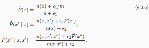
Here ϵ1,ϵ2, and ϵ3 are hyperparameters. Take ϵ1 as an example: when ϵ1=0, no smoothing is applied; when ϵ1 approaches positive infinity, P^(x) approaches the uniform probability 1/m. The above is a rather primitive variant of what other techniques can accomplish (Wood et al., 2011).
여기서 ϵ1, ϵ2 및 ϵ3은 하이퍼파라미터입니다. ϵ1을 예로 들어 보겠습니다. ϵ1=0이면 스무딩이 적용되지 않습니다. ϵ1이 양의 무한대에 접근하면 P^(x)는 균일 확률 1/m에 접근합니다. 위의 내용은 다른 기술이 수행할 수 있는 것의 다소 원시적인 변형입니다(Wood et al., 2011).
Unfortunately, models like this get unwieldy rather quickly for the following reasons. First, as discussed in Section 9.2.5, many n-grams occur very rarely, making Laplace smoothing rather unsuitable for language modeling. Second, we need to store all counts. Third, this entirely ignores the meaning of the words. For instance, “cat” and “feline” should occur in related contexts. It is quite difficult to adjust such models to additional contexts, whereas, deep learning based language models are well suited to take this into account. Last, long word sequences are almost certain to be novel, hence a model that simply counts the frequency of previously seen word sequences is bound to perform poorly there. Therefore, we focus on using neural networks for language modeling in the rest of the chapter.
불행하게도 이와 같은 모델은 다음과 같은 이유로 다소 빨리 다루기 어려워집니다. 첫째, 섹션 9.2.5에서 논의한 것처럼 많은 n-gram이 매우 드물게 발생하므로 Laplace smoothing는 언어 모델링에 적합하지 않습니다. 둘째, 모든 카운트를 저장해야 합니다. 셋째, 이것은 단어의 의미를 완전히 무시합니다. 예를 들어, "cat"과 "feline"은 관련 문맥에서 발생해야 합니다. 이러한 모델을 추가 컨텍스트에 맞게 조정하는 것은 매우 어려운 반면 딥 러닝 기반 언어 모델은 이를 고려하는 데 적합합니다. 마지막으로, 긴 단어 시퀀스는 새로운 것이 거의 확실하므로 이전에 본 단어 시퀀스의 빈도를 단순히 세는 모델은 성능이 좋지 않을 수 밖에 없습니다. 따라서 나머지 장에서는 언어 모델링을 위해 신경망을 사용하는 데 중점을 둡니다.
9.3.2. Perplexity
Next, let’s discuss about how to measure the language model quality, which will be used to evaluate our models in the subsequent sections. One way is to check how surprising the text is. A good language model is able to predict with high-accuracy tokens that what we will see next. Consider the following continuations of the phrase “It is raining”, as proposed by different language models:
다음으로, 후속 섹션에서 모델을 평가하는 데 사용될 언어 모델 품질을 측정하는 방법에 대해 논의하겠습니다. 한 가지 방법은 텍스트가 얼마나 놀라운지 확인하는 것입니다. 좋은 언어 모델은 우리가 다음에 보게 될 것을 높은 정확도의 토큰으로 예측할 수 있습니다. 다른 언어 모델에서 제안한 대로 "It is raining"이라는 구문의 다음 연속을 고려하십시오.
- “It is raining outside”
- “It is raining banana tree”
- “It is raining piouw;kcj pwepoiut”
In terms of quality, example 1 is clearly the best. The words are sensible and logically coherent. While it might not quite accurately reflect which word follows semantically (“in San Francisco” and “in winter” would have been perfectly reasonable extensions), the model is able to capture which kind of word follows. Example 2 is considerably worse by producing a nonsensical extension. Nonetheless, at least the model has learned how to spell words and some degree of correlation between words. Last, example 3 indicates a poorly trained model that does not fit data properly.
품질면에서는 예제 1이 확실히 최고입니다. 단어가 합리적이고 논리적으로 일관성이 있습니다. 어떤 단어가 의미론적으로 뒤따르는지 정확히 반영하지 못할 수도 있지만("in San Francisco"와 "in winter"는 완벽하게 합리적인 확장이었을 것입니다), 모델은 어떤 종류의 단어가 뒤에 오는지 캡처할 수 있습니다. 예제 2는 무의미한 확장을 생성하여 상당히 더 나쁩니다. 그럼에도 불구하고 적어도 모델은 단어의 철자와 단어 간의 상관 관계를 어느 정도 배웠습니다. 마지막으로 예제 3은 데이터를 제대로 맞추지 못하는 제대로 훈련되지 않은 모델을 나타냅니다.
We might measure the quality of the model by computing the likelihood of the sequence. Unfortunately this is a number that is hard to understand and difficult to compare. After all, shorter sequences are much more likely to occur than the longer ones, hence evaluating the model on Tolstoy’s magnum opus War and Peace will inevitably produce a much smaller likelihood than, say, on Saint-Exupery’s novella The Little Prince. What is missing is the equivalent of an average.
시퀀스의 우도를 계산하여 모델의 품질을 측정할 수 있습니다. 불행히도 이것은 이해하기 어렵고 비교하기 어려운 숫자입니다. 결국 짧은 시퀀스는 긴 시퀀스보다 발생할 가능성이 훨씬 더 높으므로 Tolstoy의 대작 전쟁과 평화에 대한 모델을 평가하면 필연적으로 Saint-Exupery의 소설 어린 왕자보다 훨씬 더 작은 가능성이 생성됩니다. 빠진 것은 평균과 같습니다.
Information theory comes handy here. We have defined entropy, surprisal, and cross-entropy when we introduced the softmax regression (Section 4.1.3). If we want to compress text, we can ask about predicting the next token given the current set of tokens. A better language model should allow us to predict the next token more accurately. Thus, it should allow us to spend fewer bits in compressing the sequence. So we can measure it by the cross-entropy loss averaged over all the n tokens of a sequence:
정보 이론이 여기에 유용합니다. 우리는 소프트맥스 회귀를 소개할 때 엔트로피, surprisal, 교차 엔트로피를 정의했습니다(섹션 4.1.3). 텍스트를 압축하려는 경우 현재 토큰 세트가 주어지면 다음 토큰을 예측하는 것에 대해 물어볼 수 있습니다. 더 나은 언어 모델을 사용하면 다음 토큰을 더 정확하게 예측할 수 있습니다. 따라서 시퀀스를 압축하는 데 더 적은 비트를 사용할 수 있습니다. 따라서 시퀀스의 모든 n 토큰에 대해 평균화된 교차 엔트로피 손실로 측정할 수 있습니다.
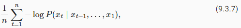
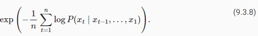
where P is given by a language model and xt is the actual token observed at time step t from the sequence. This makes the performance on documents of different lengths comparable. For historical reasons, scientists in natural language processing prefer to use a quantity called perplexity. In a nutshell, it is the exponential of (9.3.7):
여기서 P는 언어 모델에 의해 제공되고 xt는 시퀀스의 시간 단계 t에서 관찰된 실제 토큰입니다. 이것은 서로 다른 길이의 문서에 대한 성능을 비교할 수 있게 합니다. 역사적인 이유로 자연어 처리 과학자들은 당혹감이라는 양을 선호합니다. 간단히 말해서 (9.3.7)의 지수입니다.
Perplexity can be best understood as the geometric mean of the number of real choices that we have when deciding which token to pick next. Let’s look at a number of cases:
Perplexity는 다음에 선택할 토큰을 결정할 때 우리가 가진 실제 선택 수의 기하 평균으로 가장 잘 이해할 수 있습니다. 여러 가지 경우를 살펴보겠습니다.
- In the best case scenario, the model always perfectly estimates the probability of the target token as 1. In this case the perplexity of the model is 1.
- 최상의 시나리오에서 모델은 항상 대상 토큰의 확률을 1로 완벽하게 추정합니다. 이 경우 모델의 perplexity 는 1입니다.
- In the worst case scenario, the model always predicts the probability of the target token as 0. In this situation, the perplexity is positive infinity.
- 최악의 시나리오에서 모델은 항상 대상 토큰의 확률을 0으로 예측합니다. 이 상황에서 perplexity는 양의 무한대입니다.
- At the baseline, the model predicts a uniform distribution over all the available tokens of the vocabulary. In this case, the perplexity equals the number of unique tokens of the vocabulary. In fact, if we were to store the sequence without any compression, this would be the best we could do to encode it. Hence, this provides a nontrivial upper bound that any useful model must beat.
- 기준선에서 모델은 사용 가능한 모든 어휘 토큰에 대해 균일한 분포를 예측합니다. 이 경우 당도는 어휘의 고유 토큰 수와 같습니다. 사실, 압축 없이 시퀀스를 저장한다면 이것이 인코딩을 위해 할 수 있는 최선일 것입니다. 따라서 이것은 유용한 모델이 이겨야 하는 사소하지 않은 상한을 제공합니다.
Perplexity 란?
RNN에서의 퍼플렉서티(Perplexity)는 언어 모델의 성능을 평가하기 위한 지표입니다. 언어 모델은 텍스트 데이터의 다음 단어를 예측하는 작업을 수행하는데, 이때 퍼플렉서티는 모델이 텍스트 데이터 내의 다음 단어를 얼마나 잘 예측하는지를 나타내는 값입니다.
퍼플렉서티는 정보 이론에서 비용 함수(cost function)로서 사용되며, 텍스트 데이터 내의 다음 단어를 예측할 때 모델의 예측 분포와 실제 데이터의 분포 간의 차이를 측정합니다. 퍼플렉서티가 낮을수록 모델은 텍스트 데이터의 다음 단어를 더 잘 예측하고 있음을 나타냅니다.
수학적으로 퍼플렉서티는 다음과 같이 정의됩니다:
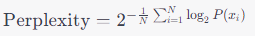
여기서:
- 은 텍스트 데이터의 총 단어 수를 나타냅니다.
- 는 실제 데이터의 번째 단어를 나타냅니다.
- 는 모델이 예측한 의 확률을 나타냅니다.
퍼플렉서티 값은 일반적으로 1보다 큰 값으로 나타나며, 낮을수록 모델의 예측 능력이 좋아진다고 판단할 수 있습니다. 따라서 RNN 언어 모델의 훈련 과정에서 퍼플렉서티를 낮추는 것이 중요한 목표 중 하나입니다.
9.3.3. Partitioning Sequences
We will design language models using neural networks and use perplexity to evaluate how good the model is at predicting the next token given the current set of tokens in text sequences. Before introducing the model, let’s assume that it processes a minibatch of sequences with predefined length at a time. Now the question is how to read minibatches of input sequences and target sequences at random.
우리는 신경망을 사용하여 언어 모델을 설계하고 perplexity를 사용하여 텍스트 시퀀스의 현재 토큰 세트가 주어진 다음 토큰을 모델이 얼마나 잘 예측하는지 평가합니다. 모델을 도입하기 전에 한 번에 미리 정의된 길이의 시퀀스 미니배치를 처리한다고 가정해 보겠습니다. 이제 문제는 입력 시퀀스와 대상 시퀀스의 미니배치를 무작위로 읽는 방법입니다.
Suppose that the dataset takes the form of a sequence of T token indices in corpus. We will partition it into subsequences, where each subsequence has n tokens (time steps). To iterate over (almost) all the tokens of the entire dataset for each epoch and obtain all possible length-n subsequences, we can introduce randomness. More concretely, at the beginning of each epoch, discard the first d tokens, where d∈[0,n) is uniformly sampled at random. The rest of the sequence is then partitioned into m=⌊(T−d)/n⌋ subsequences. Denote by xt=[xt,…,xt+n−1] the length-n subsequence starting from token xt at time step t. The resulting m partitioned subsequences are xd,xd+n,…,xd+n(m−1). Each subsequence will be used as an input sequence into the language model.
데이터 세트가 코퍼스의 T 토큰 인덱스 시퀀스 형식을 취한다고 가정합니다. 각 하위 시퀀스에는 n개의 토큰(시간 단계)이 있는 하위 시퀀스로 분할합니다. 각 시대에 대한 전체 데이터 세트의 (거의) 모든 토큰을 반복하고 가능한 모든 길이 n 하위 시퀀스를 얻기 위해 임의성을 도입할 수 있습니다. 보다 구체적으로, 각 에포크가 시작될 때 첫 번째 d 토큰을 폐기합니다. 여기서 d∈[0,n)은 무작위로 균일하게 샘플링됩니다. 나머지 시퀀스는 m=⌊(T−d)/n⌋ 하위 시퀀스로 분할됩니다. xt=[xt,…,xt+n−1]로 표시하면 시간 단계 t에서 토큰 xt에서 시작하는 길이 n 하위 시퀀스입니다. 그 결과 m개의 분할된 서브시퀀스는 xd,xd+n,…,xd+n(m−1)입니다. 각 하위 시퀀스는 언어 모델에 대한 입력 시퀀스로 사용됩니다.
For language modeling, the goal is to predict the next token based on what tokens we have seen so far, hence the targets (labels) are the original sequence, shifted by one token. The target sequence for any input sequence xt is xt+1 with length n.
언어 모델링의 경우 목표는 지금까지 본 토큰을 기반으로 다음 토큰을 예측하는 것이므로 대상(레이블)은 하나의 토큰만큼 이동된 원래 시퀀스입니다. 임의의 입력 시퀀스 xt에 대한 대상 시퀀스는 길이가 n인 xt+1입니다.
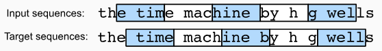
Fig. 9.3.1 shows an example of obtaining 5 pairs of input sequences and target sequences with n=5 and d=2.
그림 9.3.1은 n=5, d=2로 5쌍의 입력 시퀀스와 타겟 시퀀스를 얻은 예를 보여준다.
@d2l.add_to_class(d2l.TimeMachine)  #@save
def __init__(self, batch_size, num_steps, num_train=10000, num_val=5000):
    super(d2l.TimeMachine, self).__init__()
    self.save_hyperparameters()
    corpus, self.vocab = self.build(self._download())
    array = torch.tensor([corpus[i:i+num_steps+1]
                        for i in range(len(corpus)-num_steps)])
    self.X, self.Y = array[:,:-1], array[:,1:]
위의 코드는 TimeMachine 데이터 클래스의 __init__ 메서드를 오버라이딩하여 초기화하는 과정을 설명합니다.
- self.save_hyperparameters(): 클래스의 하이퍼파라미터를 저장합니다. 이는 모델을 학습할 때 설정한 하이퍼파라미터들을 추후에도 쉽게 참조할 수 있도록 하는 역할을 합니다.
- corpus, self.vocab = self.build(self._download()): self._download() 함수를 사용하여 Time Machine 데이터를 다운로드하고, 이를 _preprocess와 _tokenize 함수를 이용하여 전처리하고 토큰화하여 어휘를 만듭니다. 이렇게 생성된 corpus와 self.vocab은 언어 모델 학습에 필요한 데이터와 어휘 정보를 담고 있습니다.
- array = torch.tensor([corpus[i:i+num_steps+1] for i in range(len(corpus)-num_steps)]): 생성된 corpus 데이터를 이용하여 데이터 샘플을 생성합니다. num_steps만큼의 토큰으로 구성된 입력 시퀀스(X)와 그 다음의 토큰으로 구성된 출력 시퀀스(Y)를 만들어내는 과정입니다.
- self.X, self.Y = array[:,:-1], array[:,1:]: 생성된 데이터 샘플을 입력과 출력으로 나누어 저장합니다. X는 입력 시퀀스이며, 맨 마지막 토큰을 제외한 부분(array[:,:-1])을 저장하고, Y는 출력 시퀀스이며, 맨 처음 토큰을 제외한 부분(array[:,1:])을 저장합니다.
이렇게 생성된 self.X와 self.Y 데이터는 언어 모델의 학습 데이터로 사용되며, self.vocab은 학습 데이터에 포함된 토큰들에 대한 어휘 정보를 담고 있습니다.
To train language models, we will randomly sample pairs of input sequences and target sequences in minibatches. The following data loader randomly generates a minibatch from the dataset each time. The argument batch_size specifies the number of subsequence examples in each minibatch and num_steps is the subsequence length in tokens.
언어 모델을 훈련하기 위해 미니배치에서 입력 시퀀스와 대상 시퀀스 쌍을 무작위로 샘플링합니다. 다음 데이터 로더는 매번 데이터 세트에서 미니배치를 무작위로 생성합니다. 인수 batch_size는 각 미니 배치의 하위 시퀀스 예제 수를 지정하고 num_steps는 토큰의 하위 시퀀스 길이입니다.
@d2l.add_to_class(d2l.TimeMachine)  #@save
def get_dataloader(self, train):
    idx = slice(0, self.num_train) if train else slice(
        self.num_train, self.num_train + self.num_val)
    return self.get_tensorloader([self.X, self.Y], train, idx)
위의 코드는 TimeMachine 데이터 클래스의 get_dataloader 메서드를 오버라이딩하여 데이터 로더를 생성하는 과정을 설명합니다.
- idx = slice(0, self.num_train) if train else slice(self.num_train, self.num_train + self.num_val): train이 True인 경우에는 처음부터 self.num_train까지의 인덱스를 가져오고, False인 경우에는 self.num_train부터 self.num_train + self.num_val까지의 인덱스를 가져옵니다. 이로써 학습 데이터와 검증 데이터의 인덱스를 구분할 수 있습니다.
- self.get_tensorloader([self.X, self.Y], train, idx): get_tensorloader 메서드를 사용하여 데이터 샘플(self.X와 self.Y)과 인덱스를 이용하여 데이터 로더를 생성합니다. 이로써 학습 데이터와 검증 데이터에 대한 데이터 로더를 생성하게 됩니다.
이렇게 생성된 데이터 로더는 학습 데이터와 검증 데이터에 해당하는 배치를 불러올 수 있게 해주며, 언어 모델의 학습에 사용됩니다.
As we can see in the following, a minibatch of target sequences can be obtained by shifting the input sequences by one token.
다음에서 볼 수 있듯이 입력 시퀀스를 하나의 토큰으로 이동하여 대상 시퀀스의 미니 배치를 얻을 수 있습니다.
data = d2l.TimeMachine(batch_size=2, num_steps=10)
for X, Y in data.train_dataloader():
    print('X:', X, '\nY:', Y)
    break
위의 코드는 TimeMachine 데이터 클래스를 사용하여 학습 데이터의 데이터 로더를 생성하고, 첫 번째 배치를 출력하는 과정을 설명합니다.
- data = d2l.TimeMachine(batch_size=2, num_steps=10): TimeMachine 클래스의 인스턴스를 생성하고, batch_size를 2로, num_steps를 10으로 설정하여 데이터 로더를 준비합니다.
- for X, Y in data.train_dataloader():: 학습 데이터에 대한 데이터 로더를 순회하면서 각 배치를 가져옵니다.
- print('X:', X, '\nY:', Y): 각 배치의 입력 데이터 X와 대응하는 레이블 데이터 Y를 출력합니다.
- break: 첫 번째 배치만 출력하고 루프를 중단합니다.
이렇게 출력된 데이터는 언어 모델 학습에 사용되며, batch_size에 따라 한 번에 몇 개의 데이터 샘플이 처리되는지 확인할 수 있습니다. 배치의 크기가 2이기 때문에 첫 번째 배치에서 X와 Y는 각각 크기가 (2, 10)인 텐서로 출력됩니다.
X: tensor([[ 0,  5, 10, 14,  6, 15, 20, 10, 16, 15],
        [ 5, 10,  7,  7,  6, 19,  6, 15,  4,  6]])
Y: tensor([[ 5, 10, 14,  6, 15, 20, 10, 16, 15,  0],
        [10,  7,  7,  6, 19,  6, 15,  4,  6,  0]])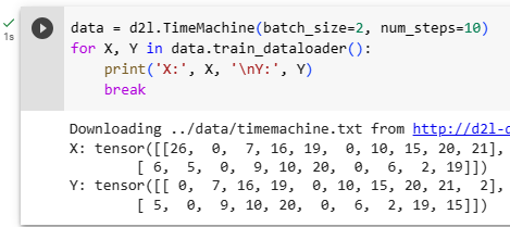
9.3.4. Summary and Discussion
Language models estimate the joint probability of a text sequence. For long sequences, n-grams provide a convenient model by truncating the dependence. However, there is a lot of structure but not enough frequency to deal with infrequent word combinations efficiently via Laplace smoothing. Thus, we will focus on neural language modeling in subsequent sections. To train language models, we can randomly sample pairs of input sequences and target sequences in minibatches. After training, we will use perplexity to measure the language model quality.
언어 모델은 텍스트 시퀀스의 공동 확률을 추정합니다. 긴 시퀀스의 경우 n-gram은 종속성을 잘라서 편리한 모델을 제공합니다. 그러나 Laplace smoothing을 통해 드물게 사용되는 단어 조합을 효율적으로 처리하기에는 구조가 많지만 빈도가 충분하지 않습니다. 따라서 후속 섹션에서 신경 언어 모델링에 중점을 둘 것입니다. 언어 모델을 훈련하기 위해 미니배치에서 입력 시퀀스와 대상 시퀀스 쌍을 무작위로 샘플링할 수 있습니다. 훈련 후에는 perplexity를 사용하여 언어 모델 품질을 측정합니다.
Language models can be scaled up with increased data size, model size, and amount in training compute. Large language models can perform desired tasks by predicting output text given input text instructions. As we will discuss later (e.g., Section 11.9), at the present moment, large language models form the basis of state-of-the-art systems across diverse tasks.
언어 모델은 증가된 데이터 크기, 모델 크기 및 교육 컴퓨팅의 양으로 확장할 수 있습니다. 대규모 언어 모델은 입력 텍스트 명령이 주어지면 출력 텍스트를 예측하여 원하는 작업을 수행할 수 있습니다. 나중에 논의하겠지만(예: 섹션 11.9) 현재 대규모 언어 모델은 다양한 작업에서 최신 시스템의 기반을 형성합니다.
Laplace smoothing 이란?
Laplace smoothing, also known as add-one smoothing or additive smoothing, is a technique used in probability and statistics to smooth the probability estimates of events that have not been observed in a given dataset. In situations where there are zero-frequency events (i.e., events that did not occur in the training data), traditional maximum likelihood estimation fails because the estimated probability for such events would be zero.
Laplace smoothing(라플라스 스무딩)은 확률 및 통계에서 사용되는 기법으로, 주어진 데이터셋에서 관측되지 않은 사건들에 대한 확률 추정치를 완화하는데 사용됩니다. 만약 학습 데이터에서 발생하지 않은 사건들이 존재하는 상황에서, 전통적인 최대 우도 추정은 해당 사건들에 대한 확률을 0으로 추정하게 되어 문제가 발생합니다.
Laplace smoothing addresses this issue by adding a small constant (usually 1) to the observed counts of each event and also adding a multiple of this constant to the denominator when calculating the probabilities. This ensures that all events have non-zero probabilities, even if they were not observed in the training data.
라플라스 스무딩은 이러한 문제를 해결하기 위해 각 사건의 관측된 빈도에 작은 상수(보통 1)를 더하고, 확률 계산시 분모에 이 상수의 배수를 더함으로써 처리합니다. 이로 인해 모든 사건들이 학습 데이터에 관계 없이 확률이 0이 아닌 값을 갖도록 보장됩니다.
Mathematically, the smoothed probability of an event is calculated as:
수학적으로, 스무딩 된 사건의 확률은 다음과 같이 계산됩니다:
P_smooth = (count(event) + k) / (total_count + k * num_events)
P_smooth = (사건 발생 횟수 + k) / (전체 사건 수 + k * 고유 사건 수)
Where:
- count(event) is the number of times the event occurred in the training data,
- 사건 발생 횟수는 학습 데이터에서 해당 사건이 발생한 횟수,
- total_count is the total number of events in the training data,
- 전체 사건 수는 학습 데이터의 전체 사건 수,
- num_events is the total number of distinct events, and
- 고유 사건 수는 모든 서로 다른 사건의 수,
- k is the smoothing parameter (usually set to 1).
- k는 스무딩 파라미터(보통 1로 설정) 입니다.
Laplace smoothing helps prevent overfitting and improves the generalization performance of probabilistic models, especially in situations where the training data is sparse or when dealing with small datasets. It is commonly used in various natural language processing tasks and other applications involving probability estimation from limited data.
라플라스 스무딩은 과적합을 방지하고, 특히 학습 데이터가 희소하거나 작은 데이터셋을 다루는 경우에 확률적 모델의 일반화 성능을 향상시키는데 도움이 됩니다. 이는 자연어 처리 작업과 확률 추정을 다루는 다양한 응용 분야에서 흔히 사용되는 기법입니다.
9.3.5. Exercises
- Suppose there are 100,000 words in the training dataset. How much word frequency and multi-word adjacent frequency does a four-gram need to store?
- How would you model a dialogue?
- What other methods can you think of for reading long sequence data?
- Consider our method for discarding a uniformly random number of the first few tokens at the beginning of each epoch.
- Does it really lead to a perfectly uniform distribution over the sequences on the document?
- What would you have to do to make things even more uniform?
- If we want a sequence example to be a complete sentence, what kind of problem does this introduce in minibatch sampling? How can we fix the problem?
'Dive into Deep Learning > D2L Recurrent Neural Networks (RNN)' 카테고리의 다른 글
| D2L - 9.7. Backpropagation Through Time (0) | 2023.08.02 |
|---|---|
| D2L - 9.6. Concise Implementation of Recurrent Neural Networks (0) | 2023.08.02 |
| D2L - 9.5. Recurrent Neural Network Implementation from Scratch (0) | 2023.08.02 |
| D2L - 9.4. Recurrent Neural Networks (0) | 2023.08.02 |
| D2L - 9.2. Converting Raw Text into Sequence Data (0) | 2023.08.01 |
| D2L - 9.1. Working with Sequences (0) | 2023.08.01 |
| D2L - 9. Recurrent Neural Networks (0) | 2023.07.31 |