

https://d2l.ai/chapter_recurrent-neural-networks/bptt.html
9.7. Backpropagation Through Time — Dive into Deep Learning 1.0.0-beta0 documentation
d2l.ai
9.7. Backpropagation Through Time
If you completed the exercises in Section 9.5, you would have seen that gradient clipping is vital to prevent the occasional massive gradients from destabilizing training. We hinted that the exploding gradients stem from backpropagating across long sequences. Before introducing a slew of modern RNN architectures, let’s take a closer look at how backpropagation works in sequence models in mathematical detail. Hopefully, this discussion will bring some precision to the notion of vanishing and exploding gradients. If you recall our discussion of forward and backward propagation through computational graphs when we introduced MLPs in Section 5.3, then forward propagation in RNNs should be relatively straightforward. Applying backpropagation in RNNs is called backpropagation through time (Werbos, 1990). This procedure requires us to expand (or unroll) the computational graph of an RNN one time step at a time. The unrolled RNN is essentially a feedforward neural network with the special property that the same parameters are repeated throughout the unrolled network, appearing at each time step. Then, just as in any feedforward neural network, we can apply the chain rule, backpropagating gradients through the unrolled net. The gradient with respect to each parameter must be summed across all places that the parameter occurs in the unrolled net. Handling such weight tying should be familiar from our chapters on convolutional neural networks.
섹션 9.5의 연습을 완료했다면 때때로 발생하는 대규모 기울기가 훈련을 불안정하게 만드는 것을 방지하기 위해 기울기 클리핑이 필수적이라는 것을 알았을 것입니다. 우리는 폭발하는 그래디언트가 긴 시퀀스에 걸쳐 역전파에서 비롯된다는 것을 암시했습니다. 수많은 최신 RNN 아키텍처를 소개하기 전에 시퀀스 모델에서 역전파가 수학적 세부 사항으로 작동하는 방식을 자세히 살펴보겠습니다. 바라건대, 이 논의가 그래디언트 소실 및 폭발의 개념에 어느 정도 정확성을 가져다 줄 것입니다. 섹션 5.3에서 MLP를 소개했을 때 계산 그래프를 통한 순방향 및 역방향 전파에 대한 논의를 기억한다면 RNN의 순방향 전파는 비교적 간단해야 합니다. RNN에서 역전파를 적용하는 것을 시간을 통한 역전파라고 합니다(Werbos, 1990). 이 절차에서는 한 번에 한 단계씩 RNN의 계산 그래프를 확장(또는 펼치기)해야 합니다. 언롤링된 RNN은 기본적으로 동일한 매개변수가 언롤링된 네트워크 전체에서 반복되어 각 시간 단계에 나타나는 특수 속성을 가진 피드포워드 신경망입니다. 그런 다음 피드포워드 신경망에서와 마찬가지로 체인 규칙을 적용하여 펼쳐진 그물을 통해 기울기를 역전파할 수 있습니다. 각 매개변수에 대한 기울기는 펼쳐진 그물에서 매개변수가 발생하는 모든 위치에서 합산되어야 합니다. 이러한 가중치 묶기를 처리하는 방법은 컨볼루션 신경망에 대한 장에서 익숙할 것입니다.
Complications arise because sequences can be rather long. It is not unusual to work with text sequences consisting of over a thousand tokens. Note that this poses problems both from a computational (too much memory) and optimization (numerical instability) standpoint. Input from the first step passes through over 1000 matrix products before arriving at the output, and another 1000 matrix products are required to compute the gradient. We now analyze what can go wrong and how to address it in practice.
시퀀스가 다소 길 수 있기 때문에 합병증이 발생합니다. 천 개가 넘는 토큰으로 구성된 텍스트 시퀀스로 작업하는 것은 드문 일이 아닙니다. 이는 계산(너무 많은 메모리) 및 최적화(수치적 불안정성) 관점에서 모두 문제를 제기합니다. 첫 번째 단계의 입력은 출력에 도달하기 전에 1000개 이상의 행렬 곱을 거치며 기울기를 계산하려면 또 다른 1000개의 행렬 곱이 필요합니다. 이제 무엇이 잘못될 수 있는지, 그리고 실제로 이를 해결하는 방법을 분석합니다.
9.7.1. Analysis of Gradients in RNNs
We start with a simplified model of how an RNN works. This model ignores details about the specifics of the hidden state and how it is updated. The mathematical notation here does not explicitly distinguish scalars, vectors, and matrices. We are just trying to develop some intuition. In this simplified model, we denote ℎt as the hidden state, xt as input, and ot as output at time step t. Recall our discussions in Section 9.4.2 that the input and the hidden state can be concatenated before being multiplied by one weight variable in the hidden layer. Thus, we use wℎ and wo to indicate the weights of the hidden layer and the output layer, respectively. As a result, the hidden states and outputs at each time steps are
RNN 작동 방식에 대한 단순화된 모델부터 시작합니다. 이 모델은 숨겨진 상태의 세부 사항과 업데이트 방법에 대한 세부 정보를 무시합니다. 여기서 수학적 표기법은 스칼라, 벡터 및 행렬을 명시적으로 구분하지 않습니다. 우리는 직관을 개발하려고 노력하고 있습니다. 이 단순화된 모델에서 우리는 ℎt를 숨겨진 상태로, xt를 입력으로, ot를 시간 단계 t에서 출력으로 나타냅니다. 섹션 9.4.2에서 입력과 은닉 상태가 은닉층에서 하나의 가중치 변수에 의해 곱해지기 전에 연결될 수 있다는 논의를 상기하십시오. 따라서 wℎ와 wo를 사용하여 숨겨진 레이어와 출력 레이어의 가중치를 각각 나타냅니다. 결과적으로 각 시간 단계의 숨겨진 상태 및 출력은 다음과 같습니다.
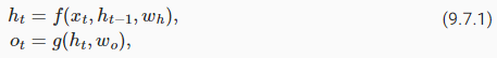
where f and g are transformations of the hidden layer and the output layer, respectively. Hence, we have a chain of values {…,(xt−1,ℎt−1,ot−1),(xt,ℎt,ot),…} that depend on each other via recurrent computation. The forward propagation is fairly straightforward. All we need is to loop through the (xt,ℎt,ot) triples one time step at a time. The discrepancy between output ot and the desired target yt is then evaluated by an objective function across all the T time steps as
여기서 f와 g는 각각 은닉층과 출력층의 변환입니다. 따라서 순환 계산을 통해 서로 의존하는 {...,(xt−1,ℎt−1,ot−1),(xt,ℎt,ot),...} 값 체인이 있습니다. 정방향 전파는 매우 간단합니다. 필요한 것은 한 번에 한 단계씩 (xt,ℎt,ot) 트리플을 반복하는 것입니다. 출력 ot와 원하는 목표 yt 사이의 불일치는 모든 T 시간 단계에서 목적 함수에 의해 다음과 같이 평가됩니다.
For backpropagation, matters are a bit trickier, especially when we compute the gradients with regard to the parameters wℎ of the objective function L. To be specific, by the chain rule,
역전파의 경우, 특히 목적 함수 L의 매개변수 wℎ에 대한 그래디언트를 계산할 때 문제가 좀 더 까다롭습니다. 구체적으로 체인 규칙에 따르면,
The first and the second factors of the product in (9.7.3) are easy to compute. The third factor ∂ℎt/∂wℎ is where things get tricky, since we need to recurrently compute the effect of the parameter wℎ on ℎt. According to the recurrent computation in (9.7.1), ℎt depends on both ℎt−1 and wℎ, where computation of ℎt−1 also depends on wℎ. Thus, evaluating the total derivate of ℎt with respect to wℎ using the chain rule yields
(9.7.3)에서 제품의 첫 번째 및 두 번째 요소는 계산하기 쉽습니다. 세 번째 요소 ∂ℎt/∂wℎ는 ℎt에 대한 매개변수 wℎ의 효과를 반복적으로 계산해야 하기 때문에 상황이 까다로워집니다. (9.7.1)의 반복 계산에 따르면 ℎt는 ℎt-1과 wℎ 모두에 의존하며, 여기서 ℎt-1의 계산도 wℎ에 의존합니다. 따라서 체인 룰을 사용하여 wℎ에 대한 ℎt의 총 도함수를 평가하면 다음과 같습니다.

To derive the above gradient, assume that we have three sequences {at},{bt},{ct} satisfying a0=0 and at=bt+ctat−1 for t=1,2,…. Then for t≥1, it is easy to show
위의 그래디언트를 도출하기 위해 t=1,2,…에 대해 a0=0 및 at=bt+ctat−1을 만족하는 세 개의 시퀀스 {at},{bt},{ct}가 있다고 가정합니다. 그런 다음 t≥1인 경우 표시하기 쉽습니다.
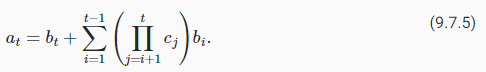
By substituting at, bt, and ct according to
다음에 따라 at, bt 및 ct를 대체하여
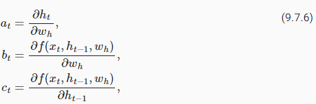
the gradient computation in (9.7.4) satisfies at=bt+ctat−1. Thus, per (9.7.5), we can remove the recurrent computation in (9.7.4) with
(9.7.4)의 그래디언트 계산은 at=bt+ctat−1을 충족합니다. 따라서 (9.7.5)에 따라 (9.7.4)에서 반복 계산을 제거할 수 있습니다.

While we can use the chain rule to compute ∂ℎt/∂wℎ recursively, this chain can get very long whenever t is large. Let’s discuss a number of strategies for dealing with this problem.
체인 규칙을 사용하여 ∂ℎt/∂wℎ를 재귀적으로 계산할 수 있지만 이 체인은 t가 클 때마다 매우 길어질 수 있습니다. 이 문제를 처리하기 위한 여러 가지 전략에 대해 논의해 봅시다.
9.7.1.1. Full Computation
One idea might be to compute the full sum in (9.7.7). However, this is very slow and gradients can blow up, since subtle changes in the initial conditions can potentially affect the outcome a lot. That is, we could see things similar to the butterfly effect, where minimal changes in the initial conditions lead to disproportionate changes in the outcome. This is generally undesirable. After all, we are looking for robust estimators that generalize well. Hence this strategy is almost never used in practice.
한 가지 아이디어는 (9.7.7)에서 전체 합계를 계산하는 것입니다. 그러나 초기 조건의 미묘한 변화가 잠재적으로 결과에 많은 영향을 미칠 수 있기 때문에 이것은 매우 느리고 기울기가 폭발할 수 있습니다. 즉, 초기 조건의 최소한의 변화가 결과에 불균형한 변화를 가져오는 나비 효과와 유사한 현상을 볼 수 있습니다. 이것은 일반적으로 바람직하지 않습니다. 결국, 우리는 잘 일반화되는 강력한 추정기를 찾고 있습니다. 따라서 이 전략은 실제로 거의 사용되지 않습니다.
9.7.1.2. Truncating Time Steps
Alternatively, we can truncate the sum in (9.7.7) after τ steps. This is what we have been discussing so far. This leads to an approximation of the true gradient, simply by terminating the sum at ∂ℎt−τ/∂wℎ. In practice this works quite well. It is what is commonly referred to as truncated backpropgation through time (Jaeger, 2002). One of the consequences of this is that the model focuses primarily on short-term influence rather than long-term consequences. This is actually desirable, since it biases the estimate towards simpler and more stable models.
또는 τ 단계 후에 합계를 (9.7.7)에서 자를 수 있습니다. 이것이 우리가 지금까지 논의한 것입니다. 이것은 단순히 ∂ℎt−τ/∂wℎ에서 합계를 종료함으로써 실제 그래디언트의 근사치로 이어집니다. 실제로 이것은 꽤 잘 작동합니다. 이것은 일반적으로 시간에 따른 절단된 역전파(truncated backpropgation)라고 합니다(Jaeger, 2002). 이것의 결과 중 하나는 모델이 장기적인 결과보다는 주로 단기적인 영향에 초점을 맞추고 있다는 것입니다. 이것은 추정치를 더 간단하고 안정적인 모델로 편향시키기 때문에 실제로 바람직합니다.
9.7.1.3. Randomized Truncation
Last, we can replace ∂ℎt/∂wℎ by a random variable which is correct in expectation but truncates the sequence. This is achieved by using a sequence of ξt with predefined 0≤πt≤1, where P(ξt=0)=1−πt and P(ξt=πt−1)=πt, thus E[ξt]=1. We use this to replace the gradient ∂ℎt/∂wℎ in (9.7.4) with
마지막으로, 우리는 ∂ℎt/∂wℎ를 예측에는 맞지만 시퀀스를 자르는 임의의 변수로 대체할 수 있습니다. 이것은 미리 정의된 0≤πt≤1을 갖는 ξt의 시퀀스를 사용하여 달성되며, 여기서 P(ξt=0)=1−πt 및 P(ξt=πt−1)=πt이므로 E[ξt]=1입니다. 이것을 사용하여 (9.7.4)의 기울기 ∂ℎt/∂wℎ를
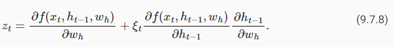
It follows from the definition of ξt that E[zt]=∂ℎt/∂wℎ. Whenever ξt=0 the recurrent computation terminates at that time step t. This leads to a weighted sum of sequences of varying lengths, where long sequences are rare but appropriately overweighted. This idea was proposed by Tallec and Ollivier (2017).
E[zt]=∂ℎt/∂wℎ는 ξt의 정의에 따른다. ξt=0일 때마다 순환 계산은 해당 시간 단계 t에서 종료됩니다. 이것은 긴 시퀀스가 드물지만 적절하게 과중한 다양한 길이의 시퀀스의 가중 합계로 이어집니다. 이 아이디어는 Tallec과 Ollivier(2017)가 제안했습니다.
9.7.1.4. Comparing Strategies
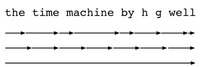
Fig. 9.7.1 illustrates the three strategies when analyzing the first few characters of The Time Machine using backpropagation through time for RNNs:
그림 9.7.1은 RNN에 대해 시간을 통한 역전파를 사용하여 The Time Machine의 처음 몇 문자를 분석할 때 세 가지 전략을 보여줍니다.
- The first row is the randomized truncation that partitions the text into segments of varying lengths.
- 첫 번째 행은 텍스트를 다양한 길이의 세그먼트로 분할하는 임의 절단입니다.
- The second row is the regular truncation that breaks the text into subsequences of the same length. This is what we have been doing in RNN experiments.
- 두 번째 행은 텍스트를 동일한 길이의 하위 시퀀스로 나누는 일반적인 잘림입니다. 이것이 우리가 RNN 실험에서 해온 것입니다.
- The third row is the full backpropagation through time that leads to a computationally infeasible expression.
- 세 번째 행은 계산적으로 실현 불가능한 표현으로 이어지는 시간에 따른 전체 역전파입니다.
Unfortunately, while appealing in theory, randomized truncation does not work much better than regular truncation, most likely due to a number of factors. First, the effect of an observation after a number of backpropagation steps into the past is quite sufficient to capture dependencies in practice. Second, the increased variance counteracts the fact that the gradient is more accurate with more steps. Third, we actually want models that have only a short range of interactions. Hence, regularly truncated backpropagation through time has a slight regularizing effect that can be desirable.
불행하게도 이론적으로는 매력적이지만 임의 절단은 여러 가지 요인으로 인해 일반 절단보다 훨씬 더 잘 작동하지 않습니다. 첫째, 과거로의 여러 역전파 단계 후 관찰 효과는 실제로 종속성을 캡처하기에 충분합니다. 둘째, 증가된 분산은 그래디언트가 더 많은 단계로 더 정확하다는 사실을 상쇄합니다. 셋째, 우리는 실제로 짧은 범위의 상호 작용만 있는 모델을 원합니다. 따라서 시간에 따라 규칙적으로 절단된 역전파는 바람직할 수 있는 약간의 규칙화 효과를 갖습니다.
9.7.2. Backpropagation Through Time in Detail
After discussing the general principle, let’s discuss backpropagation through time in detail. Different from the analysis in Section 9.7.1, in the following we will show how to compute the gradients of the objective function with respect to all the decomposed model parameters. To keep things simple, we consider an RNN without bias parameters, whose activation function in the hidden layer uses the identity mapping (ϕ(x)=x). For time step t, let the single example input and the target be xt∈ℝd and yt, respectively. The hidden state ℎt∈ℝℎ and the output ot∈ℝq are computed as
일반적인 원칙을 논의한 후 시간에 따른 역전파에 대해 자세히 논의해 봅시다. 9.7.1절의 분석과 달리 다음에서는 분해된 모든 모델 매개변수에 대한 목적 함수의 기울기를 계산하는 방법을 보여줍니다. 단순함을 유지하기 위해 편향 매개변수가 없는 RNN을 고려합니다. 숨겨진 레이어의 활성화 함수는 ID 매핑(ϕ(x)=x)을 사용합니다. 시간 단계 t의 경우 단일 예제 입력과 대상을 각각 xt∈ℝd 및 yt로 둡니다. 숨겨진 상태 ℎt∈ℝℎ와 출력 ot∈ℝq는 다음과 같이 계산됩니다.
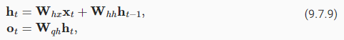
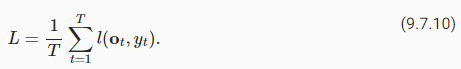
where Wℎx∈ℝℎ×d, Wℎℎ∈ℝℎ×ℎ, and Wqℎ∈ℝq×ℎ are the weight parameters. Denote by l(ot,yt) the loss at time step t. Our objective function, the loss over T time steps from the beginning of the sequence is thus
여기서 Wℎx∈ℝℎ×d, Wℎℎ∈ℝℎ×ℎ 및 Wqℎ∈ℝq×ℎ는 가중치 매개변수입니다. l(ot,yt)는 시간 단계 t에서의 손실을 나타냅니다. 우리의 목적 함수, 시퀀스 시작부터 T 시간 단계에 걸친 손실은 다음과 같습니다.
In order to visualize the dependencies among model variables and parameters during computation of the RNN, we can draw a computational graph for the model, as shown in Fig. 9.7.2. For example, the computation of the hidden states of time step 3, ℎ3, depends on the model parameters Wℎx and Wℎℎ, the hidden state of the last time step ℎ2, and the input of the current time step x3.
RNN을 계산하는 동안 모델 변수와 매개변수 간의 종속성을 시각화하기 위해 그림 9.7.2와 같이 모델에 대한 계산 그래프를 그릴 수 있습니다. 예를 들어, 시간 단계 3, ℎ3의 숨겨진 상태 계산은 모델 매개변수 Wℎx 및 Wℎℎ, 마지막 시간 단계 ℎ2의 숨겨진 상태 및 현재 시간 단계 x3의 입력에 따라 달라집니다.
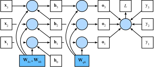
As just mentioned, the model parameters in Fig. 9.7.2 are Wℎx, Wℎℎ, and Wqℎ. Generally, training this model requires gradient computation with respect to these parameters ∂L/∂Wℎx, ∂L/∂Wℎℎ, and ∂L/∂Wqℎ. According to the dependencies in Fig. 9.7.2, we can traverse in the opposite direction of the arrows to calculate and store the gradients in turn. To flexibly express the multiplication of matrices, vectors, and scalars of different shapes in the chain rule, we continue to use the prod operator as described in Section 5.3.
방금 언급했듯이 그림 9.7.2의 모델 매개변수는 Wℎx, Wℎℎ 및 Wqℎ입니다. 일반적으로 이 모델을 훈련하려면 이러한 매개변수 ∂L/∂Wℎx, ∂L/∂Wℎℎ 및 ∂L/∂Wqℎ에 대한 그래디언트 계산이 필요합니다. 그림 9.7.2의 종속성에 따라 화살표의 반대 방향으로 순회하여 그래디언트를 차례로 계산하고 저장할 수 있습니다. 행렬, 벡터, 서로 다른 모양의 스칼라의 곱셈을 체인 룰에서 유연하게 표현하기 위해 섹션 5.3에서 설명한 대로 prod 연산자를 계속 사용합니다.
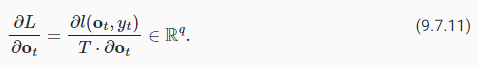
First of all, differentiating the objective function with respect to the model output at any time step t is fairly straightforward:
우선, 임의의 시간 단계 t에서 모델 출력과 관련하여 목적 함수를 미분하는 것은 매우 간단합니다.
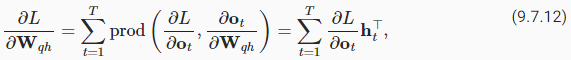
Now, we can calculate the gradient of the objective with respect to the parameter Wqℎ in the output layer: ∂L/∂Wqℎ∈ℝq×ℎ. Based on Fig. 9.7.2, the objective L depends on Wqℎ via o1,…,oT. Using the chain rule yields where ∂L//∂ot is given by (9.7.11).
이제 출력 레이어의 매개변수 Wqℎ에 대한 목표 기울기를 계산할 수 있습니다: ∂L/∂Wqℎ∈ℝq×ℎ. 그림 9.7.2에 따라 목표 L은 o1,…,oT를 통해 Wqℎ에 따라 달라집니다. 체인 규칙을 사용하면 ∂L//∂ot가 (9.7.11)에 의해 제공됩니다.
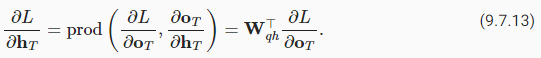
Next, as shown in Fig. 9.7.2, at the final time step T, the objective function L depends on the hidden state ℎT only via oT. Therefore, we can easily find the gradient ∂L/∂ℎt∈ℝℎ using the chain rule:
다음으로 그림 9.7.2에서와 같이 최종 시간 단계 T에서 목적 함수 L은 oT를 통해서만 숨겨진 상태 ℎT에 의존합니다. 따라서 체인 규칙을 사용하여 기울기 ∂L/∂ℎt∈ℝℎ를 쉽게 찾을 수 있습니다.
It gets trickier for any time step t<T, where the objective function L depends on ℎt via ℎt+1 and ot. According to the chain rule, the gradient of the hidden state ∂L/ ∂ℎt∈ℝℎ at any time step t<T can be recurrently computed as:
목적 함수 L이 ℎt+1 및 ot를 통해 ℎt에 의존하는 임의의 시간 단계 t<T에 대해 더 까다로워집니다. 체인 규칙에 따라 임의의 시간 단계 t<T에서 숨겨진 상태 ∂L/ ∂ℎt∈ℝℎ의 기울기는 다음과 같이 반복적으로 계산할 수 있습니다.

For analysis, expanding the recurrent computation for any time step 1≤t≤T gives
분석을 위해 임의의 시간 단계 1≤t≤T에 대한 반복 계산을 확장하면 다음이 제공됩니다.
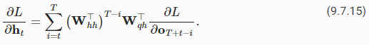
We can see from (9.7.15) that this simple linear example already exhibits some key problems of long sequence models: it involves potentially very large powers of Wℎℎ⊤. In it, eigenvalues smaller than 1 vanish and eigenvalues larger than 1 diverge. This is numerically unstable, which manifests itself in the form of vanishing and exploding gradients. One way to address this is to truncate the time steps at a computationally convenient size as discussed in Section 9.7.1. In practice, this truncation can also be effected by detaching the gradient after a given number of time steps. Later on, we will see how more sophisticated sequence models such as long short-term memory can alleviate this further.
우리는 (9.7.15)에서 이 간단한 선형 예제가 이미 긴 시퀀스 모델의 몇 가지 주요 문제를 보여주고 있음을 알 수 있습니다. 잠재적으로 매우 큰 Wℎℎ⊤의 거듭제곱이 관련됩니다. 그 안에서 1보다 작은 고유값은 사라지고 1보다 큰 고유값은 발산한다. 이것은 수치적으로 불안정하며 기울기가 사라지고 폭발하는 형태로 나타납니다. 이 문제를 해결하는 한 가지 방법은 섹션 9.7.1에서 설명한 것처럼 계산상 편리한 크기로 시간 단계를 자르는 것입니다. 실제로 이 잘림은 주어진 시간 단계 수 후에 기울기를 분리하여 영향을 줄 수도 있습니다. 나중에 우리는 장단기 기억과 같은 더 정교한 시퀀스 모델이 이것을 어떻게 더 완화할 수 있는지 보게 될 것입니다.
Finally, Fig. 9.7.2 shows that the objective function L depends on model parameters Wℎx and Wℎℎ in the hidden layer via hidden states ℎ1,…,ℎT. To compute gradients with respect to such parameters ∂L/∂Wℎx∈ℝℎ×d and L/∂Wℎℎ∈ℝℎ×ℎ, we apply the chain rule that gives
마지막으로 그림 9.7.2는 목적 함수 L이 숨겨진 상태 ℎ1,… 이러한 매개변수 ∂L/∂Wℎx∈ℝℎ×d 및 L/∂Wℎℎ∈ℝℎ×ℎ와 관련하여 기울기를 계산하기 위해 다음과 같은 체인 규칙을 적용합니다.
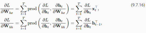
where ∂L/∂ℎt that is recurrently computed by (9.7.13) and (9.7.14) is the key quantity that affects the numerical stability.
여기서 (9.7.13)과 (9.7.14)에 의해 반복적으로 계산되는 ∂L/∂ℎt는 수치 안정성에 영향을 미치는 핵심 수량입니다.
Since backpropagation through time is the application of backpropagation in RNNs, as we have explained in Section 5.3, training RNNs alternates forward propagation with backpropagation through time. Besides, backpropagation through time computes and stores the above gradients in turn. Specifically, stored intermediate values are reused to avoid duplicate calculations, such as storing ∂L/∂ℎt to be used in computation of both ∂L/∂Wℎx and ∂L/∂Wℎℎ.
시간을 통한 역전파는 RNN에서 역전파를 적용한 것이므로 섹션 5.3에서 설명한 것처럼 훈련 RNN은 순방향 전파와 시간을 통한 역전파를 번갈아 사용합니다. 게다가, 시간을 통한 역전파는 위의 그래디언트를 차례로 계산하고 저장합니다. 구체적으로, ∂L/∂Wℎx 및 ∂L/∂Wℎℎ의 계산에 사용되는 ∂L/∂ℎt를 저장하는 것과 같이, 저장된 중간 값은 중복 계산을 피하기 위해 재사용됩니다.
9.7.3. Summary
Backpropagation through time is merely an application of backpropagation to sequence models with a hidden state. Truncation is needed for computational convenience and numerical stability, such as regular truncation and randomized truncation. High powers of matrices can lead to divergent or vanishing eigenvalues. This manifests itself in the form of exploding or vanishing gradients. For efficient computation, intermediate values are cached during backpropagation through time.
시간에 따른 역전파는 은닉 상태의 시퀀스 모델에 역전파를 적용한 것일 뿐입니다. Truncation은 regular truncation, randomized truncation과 같이 계산의 편리성과 수치적 안정성을 위해 필요합니다. 행렬의 거듭제곱이 높으면 고유값이 발산하거나 사라질 수 있습니다. 이는 그라데이션이 폭발하거나 사라지는 형태로 나타납니다. 효율적인 계산을 위해 시간을 통해 역전파하는 동안 중간 값이 캐시됩니다.
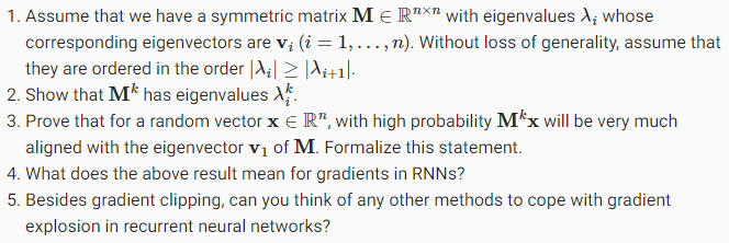
9.7.4. Exercises
'Dive into Deep Learning > D2L Recurrent Neural Networks (RNN)' 카테고리의 다른 글
| D2L - 9.6. Concise Implementation of Recurrent Neural Networks (0) | 2023.08.02 |
|---|---|
| D2L - 9.5. Recurrent Neural Network Implementation from Scratch (0) | 2023.08.02 |
| D2L - 9.4. Recurrent Neural Networks (0) | 2023.08.02 |
| D2L - 9.3. Language Models (0) | 2023.08.02 |
| D2L - 9.2. Converting Raw Text into Sequence Data (0) | 2023.08.01 |
| D2L - 9.1. Working with Sequences (0) | 2023.08.01 |
| D2L - 9. Recurrent Neural Networks (0) | 2023.07.31 |