

https://d2l.ai/chapter_recurrent-neural-networks/rnn.html
9.4. Recurrent Neural Networks — Dive into Deep Learning 1.0.0-beta0 documentation
d2l.ai
9.4. Recurrent Neural Networks
In Section 9.3 we described Markov models and n-grams for language modeling, where the conditional probability of token xt at time step t only depends on the n−1 previous tokens. If we want to incorporate the possible effect of tokens earlier than time step t−(n−1) on xt, we need to increase n. However, the number of model parameters would also increase exponentially with it, as we need to store |V|n numbers for a vocabulary set V. Hence, rather than modeling P(xt∣xt−1,…,xt−n+1) it is preferable to use a latent variable model:
섹션 9.3에서 우리는 언어 모델링을 위한 Markov 모델과 n-그램을 설명했습니다. 여기서 시간 단계 t에서 토큰 xt의 조건부 확률은 n-1 이전 토큰에만 의존합니다. xt에 대한 시간 단계 t-(n-1) 이전의 토큰의 가능한 효과를 통합하려면 n을 증가시켜야 합니다. 그러나 어휘 집합 V에 대해 |V|n 숫자를 저장해야 하므로 모델 매개변수의 수도 기하급수적으로 증가합니다. 따라서 P(xt∣xt−1,…,xt−n+1을 모델링하는 대신 ) 잠재 변수 모델을 사용하는 것이 바람직합니다.

where ℎt−1 is a hidden state that stores the sequence information up to time step t−1. In general, the hidden state at any time step t could be computed based on both the current input xt and the previous hidden state ℎt−1:
여기서 ℎt-1은 시간 단계 t-1까지의 시퀀스 정보를 저장하는 숨겨진 상태입니다. 일반적으로 t단계의 숨겨진 상태는 현재 입력 xt와 이전 숨겨진 상태 ℎt-1을 기반으로 계산할 수 있습니다.

For a sufficiently powerful function f in (9.4.2), the latent variable model is not an approximation. After all, ℎt may simply store all the data it has observed so far. However, it could potentially make both computation and storage expensive.
(9.4.2)의 충분히 강력한 함수 f의 경우 잠재 변수 모델은 근사치가 아닙니다. 결국 ℎt는 지금까지 관찰한 모든 데이터를 단순히 저장할 수 있습니다. 그러나 잠재적으로 계산과 저장 비용이 모두 비쌀 수 있습니다.
Recall that we have discussed hidden layers with hidden units in Section 5. It is noteworthy that hidden layers and hidden states refer to two very different concepts. Hidden layers are, as explained, layers that are hidden from view on the path from input to output. Hidden states are technically speaking inputs to whatever we do at a given step, and they can only be computed by looking at data at previous time steps.
섹션 5에서 은닉 유닛이 있는 은닉층에 대해 논의한 것을 상기하십시오. 은닉층과 은닉 상태는 매우 다른 두 가지 개념을 나타냅니다. 숨겨진 레이어는 설명된 대로 입력에서 출력까지의 경로에서 보기에서 숨겨진 레이어입니다. 숨겨진 상태는 기술적으로 주어진 단계에서 수행하는 모든 작업에 대한 입력이며 이전 시간 단계의 데이터를 확인해야만 계산할 수 있습니다.
Recurrent neural networks (RNNs) are neural networks with hidden states. Before introducing the RNN model, we first revisit the MLP model introduced in Section 5.1.
순환 신경망(RNN)은 숨겨진 상태가 있는 신경망입니다. RNN 모델을 소개하기 전에 먼저 섹션 5.1에서 소개한 MLP 모델을 다시 살펴보겠습니다.
import torch
from d2l import torch as d2l
9.4.1. Neural Networks without Hidden States
Let’s take a look at an MLP with a single hidden layer. Let the hidden layer’s activation function be ϕ. Given a minibatch of examples X∈Rn×d with batch size n and d inputs, the hidden layer output H∈Rn×ℎ is calculated as
단일 히든 레이어가 있는 MLP를 살펴보겠습니다. 은닉층의 활성화 함수를 φ라 하자. 배치 크기가 n이고 입력이 d인 예제 X∈Rn×d의 미니 배치가 주어지면 숨겨진 계층 출력 H∈Rn×ℎ는 다음과 같이 계산됩니다.

In (9.4.3), we have the weight parameter Wxℎ∈Rd×ℎ, the bias parameter bℎ∈R1×ℎ, and the number of hidden units ℎ, for the hidden layer. Thus, broadcasting (see Section 2.1.4) is applied during the summation. Next, the hidden layer output H is used as input of the output layer. The output layer is given by
(9.4.3)에서 은닉 계층에 대한 가중치 매개변수 Wxℎ∈Rd×ℎ, 편향 매개변수 bℎ∈R1×ℎ 및 은닉 유닛의 수 ℎ가 있습니다. 따라서 브로드캐스팅(섹션 2.1.4 참조)은 합산 중에 적용됩니다. 다음으로 숨겨진 레이어 출력 H는 출력 레이어의 입력으로 사용됩니다. 출력 레이어는 다음과 같이 지정됩니다.

where O∈Rn×q is the output variable, Wℎq∈Rℎ×q is the weight parameter, and bq∈R1×q is the bias parameter of the output layer. If it is a classification problem, we can use softmax(O) to compute the probability distribution of the output categories.
여기서 O∈Rn×q는 출력 변수, Wℎq∈Rℎ×q는 가중치 매개변수, bq∈R1×q는 출력 레이어의 편향 매개변수입니다. 분류 문제인 경우 softmax(O)를 사용하여 출력 범주의 확률 분포를 계산할 수 있습니다.
This is entirely analogous to the regression problem we solved previously in Section 9.1, hence we omit details. Suffice it to say that we can pick feature-label pairs at random and learn the parameters of our network via automatic differentiation and stochastic gradient descent.
이것은 섹션 9.1에서 이전에 해결한 회귀 문제와 완전히 유사하므로 세부 사항을 생략합니다. 기능 레이블 쌍을 무작위로 선택하고 자동 미분 및 확률적 경사 하강법을 통해 네트워크의 매개변수를 학습할 수 있다고 말하는 것으로 충분합니다.
Hidden Layer와 Hidden State.
In the context of Recurrent Neural Networks (RNNs), both "hidden layer" and "hidden state" are terms that refer to specific concepts within the architecture of the network. However, they represent different aspects of how information is processed and propagated through the network.
RNN(순환 신경망)의 맥락에서 "은닉 레이어(hidden layer)"와 "은닉 상태(hidden state)"는 네트워크의 아키텍처 내에서 특정 개념을 나타내는 용어입니다. 그러나 이들은 정보가 어떻게 처리되고 전달되는지에 대한 다른 측면을 나타냅니다.
- Hidden Layer: The term "hidden layer" in an RNN generally refers to the layer of neurons that exist between the input layer and the output layer. These neurons are responsible for capturing and transforming the input data into a format that is suitable for making predictions or generating outputs. In the case of an RNN, the hidden layer is the part of the network where the temporal or sequential information is captured. Each neuron in the hidden layer takes as input the data from the input layer and its own previous state, and produces an output that is then passed to the next time step. Essentially, the hidden layer processes input data and passes relevant information forward through time.
RNN의 "은닉 레이어"는 일반적으로 입력 레이어와 출력 레이어 사이에 있는 뉴런의 레이어를 가리킵니다. 이러한 뉴런은 입력 데이터를 적절한 형식으로 변환하고 변환하는 역할을 담당합니다. RNN의 경우 은닉 레이어는 시간적 또는 순차적 정보가 포착되는 부분입니다. 은닉 레이어의 각 뉴런은 입력 레이어의 데이터와 이전 상태를 입력으로 받아들이고 다음 시간 단계로 전달될 출력을 생성합니다. 기본적으로 은닉 레이어는 입력 데이터를 처리하고 관련 정보를 시간을 통해 전달합니다. - Hidden State: The "hidden state," on the other hand, refers specifically to the output that is generated by the hidden layer of an RNN at a particular time step. It contains the processed information that the RNN has learned from the sequence of inputs up to that point. This hidden state is then used as input for the next time step, along with the input data at that time step. In essence, the hidden state encapsulates the network's memory or understanding of the sequence up to the current time step.
반면에 "은닉 상태"는 특정 시간 단계에서 RNN의 은닉 레이어가 생성하는 출력을 지칭합니다. 이 은닉 상태는 해당 지점까지의 입력 시퀀스로부터 학습한 처리된 정보를 포함합니다. 이 은닉 상태는 다음 시간 단계의 입력과 함께 다음 시간 단계로 전달됩니다. 본질적으로 은닉 상태는 네트워크의 메모리 또는 현재 시간 단계까지의 시퀀스를 나타내며 다음 시간 단계의 입력 역할을 합니다.
In summary, the hidden layer is a conceptual layer within the architecture of the RNN that performs computations to process and transform input data over time, while the hidden state is the actual output or representation produced by the hidden layer at a specific time step, which serves as both the network's memory and input for the next time step.
요약하면, 은닉 레이어는 RNN 아키텍처 내에서 계산을 수행하여 시간에 따라 입력 데이터를 처리하고 변환하는 개념적인 레이어입니다. 반면 은닉 상태는 특정 시간 단계에서 은닉 레이어가 생성하는 실제 출력 또는 표현이며 네트워크의 메모리 역할과 다음 시간 단계의 입력 역할을 동시에 수행합니다.
9.4.2. Recurrent Neural Networks with Hidden States
Matters are entirely different when we have hidden states. Let’s look at the structure in some more detail.
숨겨진 상태가 있을 때는 문제가 완전히 다릅니다. 구조를 좀 더 자세히 살펴보겠습니다.
Assume that we have a minibatch of inputs Xt∈Rn×d at time step t. In other words, for a minibatch of n sequence examples, each row of Xt corresponds to one example at time step t from the sequence. Next, denote by Ht∈Rn×ℎ the hidden layer output of time step t. Unlike the MLP, here we save the hidden layer output Ht−1 from the previous time step and introduce a new weight parameter Wℎℎ∈Rℎ×ℎ to describe how to use the hidden layer output of the previous time step in the current time step. Specifically, the calculation of the hidden layer output of the current time step is determined by the input of the current time step together with the hidden layer output of the previous time step:
시간 단계 t에서 입력 Xt∈Rn×d의 미니배치가 있다고 가정합니다. 다시 말해, n 시퀀스 예제의 미니배치에 대해 Xt의 각 행은 시퀀스의 시간 단계 t에서 하나의 예제에 해당합니다. 다음으로 시간 단계 t의 숨겨진 레이어 출력을 Ht∈Rn×ℎ로 표시합니다. MLP와 달리 여기서는 이전 시간 단계의 숨겨진 계층 출력 Ht-1을 저장하고 현재 시간 단계에서 이전 시간 단계의 숨겨진 계층 출력을 사용하는 방법을 설명하기 위해 새로운 가중치 매개변수 Wℎℎ∈Rℎ×ℎ를 도입합니다. 특히, 현재 시간 단계의 은닉층 출력 계산은 이전 시간 단계의 은닉층 출력과 함께 현재 시간 단계의 입력에 의해 결정됩니다.

Compared with (9.4.3), (9.4.5) adds one more term Ht−1Wℎℎ and thus instantiates (9.4.2). From the relationship between hidden layer outputs Ht and Ht−1 of adjacent time steps, we know that these variables captured and retained the sequence’s historical information up to their current time step, just like the state or memory of the neural network’s current time step. Therefore, such a hidden layer output is called a hidden state. Since the hidden state uses the same definition of the previous time step in the current time step, the computation of (9.4.5) is recurrent. Hence, as we said, neural networks with hidden states based on recurrent computation are named recurrent neural networks. Layers that perform the computation of (9.4.5) in RNNs are called recurrent layers.
(9.4.3)과 비교하여 (9.4.5)는 Ht−1Wℎℎ 항을 하나 더 추가하여 (9.4.2)를 인스턴스화합니다. 인접한 시간 단계의 숨겨진 레이어 출력 Ht와 Ht-1 사이의 관계에서 우리는 이러한 변수가 신경망의 현재 시간 단계의 상태 또는 메모리와 마찬가지로 현재 시간 단계까지 시퀀스의 과거 정보를 캡처하고 유지한다는 것을 알고 있습니다. 따라서 이러한 은닉층 출력을 은닉 상태(hidden state)라고 합니다. 숨겨진 상태는 현재 시간 단계에서 이전 시간 단계의 동일한 정의를 사용하므로 (9.4.5)의 계산이 반복됩니다. 따라서 우리가 말했듯이 순환 계산을 기반으로 하는 숨겨진 상태가 있는 신경망을 순환 신경망이라고 합니다. RNN에서 (9.4.5)의 계산을 수행하는 계층을 순환 계층이라고 합니다.
There are many different ways for constructing RNNs. RNNs with a hidden state defined by (9.4.5) are very common. For time step t, the output of the output layer is similar to the computation in the MLP:
RNN을 구성하는 방법에는 여러 가지가 있습니다. (9.4.5)로 정의된 숨겨진 상태가 있는 RNN은 매우 일반적입니다. 시간 단계 t의 경우 출력 계층의 출력은 MLP의 계산과 유사합니다.

Parameters of the RNN include the weights Wxℎ∈Rd×ℎ,Wℎℎ∈Rℎ×ℎ, and the bias bℎ∈R1×ℎ of the hidden layer, together with the weights Wℎq∈Rℎ×q and the bias bq∈R1×q of the output layer. It is worth mentioning that even at different time steps, RNNs always use these model parameters. Therefore, the parameterization cost of an RNN does not grow as the number of time steps increases.
RNN의 파라미터에는 가중치 Wxℎ∈Rd×ℎ, Wℎℎ∈Rℎ×ℎ, 숨겨진 레이어의 바이어스 bℎ∈R1×ℎ, 가중치 Wℎq∈Rℎ×q 및 바이어스 bq∈R1×q가 포함됩니다. 출력 레이어. 다른 시간 단계에서도 RNN은 항상 이러한 모델 매개변수를 사용한다는 점을 언급할 가치가 있습니다. 따라서 RNN의 매개변수화 비용은 시간 단계가 증가해도 증가하지 않습니다.
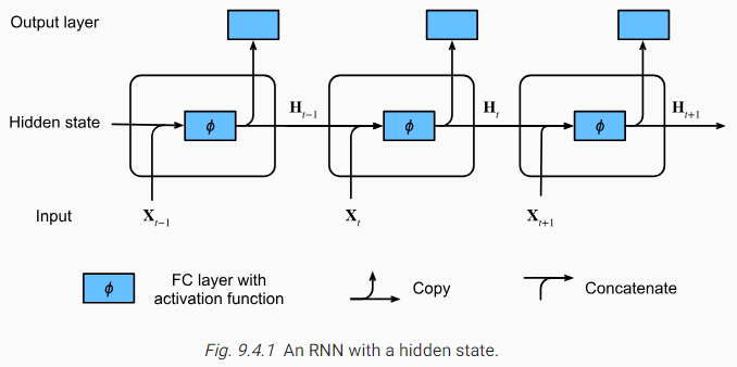
Fig. 9.4.1 illustrates the computational logic of an RNN at three adjacent time steps. At any time step t, the computation of the hidden state can be treated as: (i) concatenating the input Xt at the current time step t and the hidden state Ht−1 at the previous time step t−1; (ii) feeding the concatenation result into a fully connected layer with the activation function ϕ. The output of such a fully connected layer is the hidden state Ht of the current time step t. In this case, the model parameters are the concatenation of Wxℎ and Wℎℎ, and a bias of bℎ, all from (9.4.5). The hidden state of the current time step t, Ht, will participate in computing the hidden state Ht+1 of the next time step t+1. What is more, Ht will also be fed into the fully connected output layer to compute the output Ot of the current time step t.
그림 9.4.1은 세 개의 인접한 시간 단계에서 RNN의 계산 논리를 보여줍니다. 임의의 시간 단계 t에서 숨겨진 상태의 계산은 다음과 같이 처리될 수 있습니다. (i) 현재 시간 단계 t의 입력 Xt와 이전 시간 단계 t-1의 숨겨진 상태 Ht-1을 연결합니다. (ii) 연결 결과를 활성화 함수 φ와 함께 완전히 연결된 레이어에 공급합니다. 이러한 완전 연결 계층의 출력은 현재 시간 단계 t의 숨겨진 상태 Ht입니다. 이 경우 모델 매개변수는 모두 (9.4.5)에서 Wxℎ와 Wℎℎ의 연결과 bℎ의 바이어스입니다. 현재 시간 단계 t의 은닉 상태인 Ht는 다음 시간 단계 t+1의 은닉 상태 Ht+1을 계산하는 데 참여합니다. 또한 Ht는 현재 시간 단계 t의 출력 Ot를 계산하기 위해 완전히 연결된 출력 계층에 공급됩니다.
We just mentioned that the calculation of XtWxℎ+Ht−1Wℎℎ for the hidden state is equivalent to matrix multiplication of concatenation of Xt and Ht−1 and concatenation of Wxℎ and Wℎℎ. Though this can be proven in mathematics, in the following we just use a simple code snippet to show this. To begin with, we define matrices X, W_xh, H, and W_hh, whose shapes are (3, 1), (1, 4), (3, 4), and (4, 4), respectively. Multiplying X by W_xh, and H by W_hh, respectively, and then adding these two multiplications, we obtain a matrix of shape (3, 4).
은닉 상태에 대한 XtWxℎ+Ht−1Wℎℎ의 계산은 Xt와 Ht−1의 연결 및 Wxℎ와 Wℎℎ의 연결의 행렬 곱셈과 동일하다고 언급했습니다. 이것은 수학에서 증명될 수 있지만 다음에서는 이를 보여주기 위해 간단한 코드 스니펫을 사용합니다. 우선, 모양이 각각 (3, 1), (1, 4), (3, 4) 및 (4, 4)인 행렬 X, W_xh, H 및 W_hh를 정의합니다. X에 W_xh를 곱하고 H에 W_hh를 각각 곱한 다음 이 두 곱을 더하면 모양이 (3, 4)인 행렬을 얻습니다.
X, W_xh = torch.randn(3, 1), torch.randn(1, 4)
H, W_hh = torch.randn(3, 4), torch.randn(4, 4)
torch.matmul(X, W_xh) + torch.matmul(H, W_hh)
위 코드는 순환 신경망(RNN)의 순전파 계산을 수행하는 예시입니다. 간단한 RNN 구조에서 입력과 숨겨진 상태의 선형 결합을 통해 새로운 숨겨진 상태를 계산하는 과정을 나타냅니다.
여기서 X는 입력 벡터이며, W_xh는 입력에서 숨겨진 상태로의 가중치 행렬입니다. H는 현재 숨겨진 상태 벡터이며, W_hh는 숨겨진 상태에서 다음 숨겨진 상태로의 가중치 행렬입니다.
torch.matmul(X, W_xh)는 입력과 입력에서 숨겨진 상태로의 가중치 행렬의 곱을 나타내며, torch.matmul(H, W_hh)는 현재 숨겨진 상태와 숨겨진 상태에서 다음 숨겨진 상태로의 가중치 행렬의 곱을 나타냅니다.
두 결과를 더하면, 새로운 숨겨진 상태를 계산할 수 있습니다. 이러한 선형 결합은 RNN의 기본 동작을 나타내며, 숨겨진 상태의 변화를 기반으로 다음 숨겨진 상태를 예측하거나 추론하는 과정을 반복하여 시퀀스 데이터를 처리하는 데 사용됩니다.
tensor([[-1.6464, -8.4141,  1.5096,  3.9953],
        [-1.2590, -0.2353,  2.5025,  0.2107],
        [-2.5954,  0.8102, -1.3280, -1.1265]])
Now we concatenate the matrices X and H along columns (axis 1), and the matrices W_xh and W_hh along rows (axis 0). These two concatenations result in matrices of shape (3, 5) and of shape (5, 4), respectively. Multiplying these two concatenated matrices, we obtain the same output matrix of shape (3, 4) as above.
이제 열(축 1)을 따라 행렬 X와 H를 연결하고 행(축 0)을 따라 행렬 W_xh와 W_hh를 연결합니다. 이 두 연결은 각각 형태 (3, 5) 및 형태 (5, 4)의 행렬을 생성합니다. 이 두 개의 연결된 행렬을 곱하면 위와 같은 (3, 4) 모양의 동일한 출력 행렬을 얻습니다.
torch.matmul(torch.cat((X, H), 1), torch.cat((W_xh, W_hh), 0))위 코드는 두 개의 입력을 연결하고 이에 대해 가중치 행렬의 곱을 계산하는 과정을 나타냅니다. 이 코드는 순환 신경망(RNN)에서 입력과 이전 숨겨진 상태를 함께 고려하여 새로운 숨겨진 상태를 계산하는 것을 표현합니다.
여기서 X는 입력 벡터, H는 현재 숨겨진 상태 벡터입니다. 두 개의 행렬을 각각 가로 방향으로 연결하고, 연결된 행렬에 가중치 행렬의 곱을 수행합니다.
torch.cat((X, H), 1)은 입력 벡터 X와 현재 숨겨진 상태 벡터 H를 가로 방향으로 연결한 행렬을 생성합니다. 마찬가지로, torch.cat((W_xh, W_hh), 0)은 입력에서 숨겨진 상태로의 가중치 행렬 W_xh와 숨겨진 상태에서 다음 숨겨진 상태로의 가중치 행렬 W_hh를 세로 방향으로 연결한 행렬을 생성합니다.
연결된 입력과 가중치 행렬을 곱하면, 입력과 이전 숨겨진 상태를 고려한 새로운 숨겨진 상태가 계산됩니다. 이러한 과정은 RNN에서 시퀀스 데이터를 처리하고 이전 상태의 정보를 유지하는 데 사용됩니다.
tensor([[-1.6464, -8.4141,  1.5096,  3.9953],
        [-1.2590, -0.2353,  2.5025,  0.2107],
        [-2.5954,  0.8102, -1.3280, -1.1265]])
9.4.3. RNN-based Character-Level Language Models
Recall that for language modeling in Section 9.3, we aim to predict the next token based on the current and past tokens, thus we shift the original sequence by one token as the targets (labels). Bengio et al. (2003) first proposed to use a neural network for language modeling. In the following we illustrate how RNNs can be used to build a language model. Let the minibatch size be one, and the sequence of the text be “machine”. To simplify training in subsequent sections, we tokenize text into characters rather than words and consider a character-level language model. Fig. 9.4.2 demonstrates how to predict the next character based on the current and previous characters via an RNN for character-level language modeling.
섹션 9.3의 언어 모델링의 경우 현재 및 과거 토큰을 기반으로 다음 토큰을 예측하는 것을 목표로 하므로 원래 시퀀스를 대상(레이블)으로 한 토큰만큼 이동합니다. Bengioet al. (2003)은 언어 모델링을 위해 신경망을 사용하는 것을 처음 제안했습니다. 다음에서는 RNN을 사용하여 언어 모델을 구축하는 방법을 설명합니다. 미니 배치 크기를 1로 하고 텍스트의 순서를 "machine"로 설정합니다. 후속 섹션에서 교육을 단순화하기 위해 텍스트를 단어가 아닌 문자로 토큰화하고 문자 수준 언어 모델을 고려합니다. 그림 9.4.2는 문자 수준 언어 모델링을 위해 RNN을 통해 현재 및 이전 문자를 기반으로 다음 문자를 예측하는 방법을 보여줍니다.
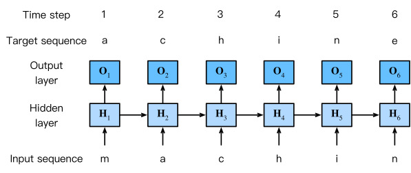
During the training process, we run a softmax operation on the output from the output layer for each time step, and then use the cross-entropy loss to compute the error between the model output and the target. Due to the recurrent computation of the hidden state in the hidden layer, the output of time step 3 in Fig. 9.4.2, O3, is determined by the text sequence “m”, “a”, and “c”. Since the next character of the sequence in the training data is “h”, the loss of time step 3 will depend on the probability distribution of the next character generated based on the feature sequence “m”, “a”, “c” and the target “h” of this time step.
training 프로세스 중에 각 시간 단계에 대해 출력 레이어의 출력에 대해 소프트맥스 작업을 실행한 다음 교차 엔트로피 손실을 사용하여 모델 출력과 대상 간의 오류를 계산합니다. 은닉층에서 은닉 상태의 반복 계산으로 인해 그림 9.4.2의 시간 단계 3인 O3의 출력은 텍스트 시퀀스 "m", "a" 및 "c"에 의해 결정됩니다. 학습 데이터에서 시퀀스의 다음 문자가 "h"이므로 시간 단계 3의 손실은 특징 시퀀스 "m", "a", "c" 및 이 시간 단계의 목표 "h".
In practice, each token is represented by a d-dimensional vector, and we use a batch size n>1. Therefore, the input Xt at time step t will be a n×d matrix, which is identical to what we discussed in Section 9.4.2.
실제로 각 토큰은 d차원 벡터로 표현되며 배치 크기 n>1을 사용합니다. 따라서 시간 단계 t에서의 입력 Xt는 n×d 행렬이 될 것이며 이는 섹션 9.4.2에서 논의한 것과 동일합니다.
In the following sections, we will implement RNNs for character-level language models.
다음 섹션에서는 문자 수준 언어 모델을 위한 RNN을 구현합니다.
9.4.4. Summary
A neural network that uses recurrent computation for hidden states is called a recurrent neural network (RNN). The hidden state of an RNN can capture historical information of the sequence up to the current time step. With recurrent computation, the number of RNN model parameters does not grow as the number of time steps increases. As for applications, an RNN can be used to create character-level language models.
은닉 상태에 대해 반복 계산을 사용하는 신경망을 순환 신경망(RNN)이라고 합니다. RNN의 숨겨진 상태는 현재 시간 단계까지 시퀀스의 과거 정보를 캡처할 수 있습니다. 반복 계산을 사용하면 RNN 모델 매개변수의 수는 시간 단계의 수가 증가해도 증가하지 않습니다. 애플리케이션의 경우 RNN을 사용하여 문자 수준 언어 모델을 만들 수 있습니다.
9.4.5. Exercises
- If we use an RNN to predict the next character in a text sequence, what is the required dimension for any output?
- Why can RNNs express the conditional probability of a token at some time step based on all the previous tokens in the text sequence?
- What happens to the gradient if you backpropagate through a long sequence?
- What are some of the problems associated with the language model described in this section?
'Dive into Deep Learning > D2L Recurrent Neural Networks (RNN)' 카테고리의 다른 글
| D2L - 9.7. Backpropagation Through Time (0) | 2023.08.02 |
|---|---|
| D2L - 9.6. Concise Implementation of Recurrent Neural Networks (0) | 2023.08.02 |
| D2L - 9.5. Recurrent Neural Network Implementation from Scratch (0) | 2023.08.02 |
| D2L - 9.3. Language Models (0) | 2023.08.02 |
| D2L - 9.2. Converting Raw Text into Sequence Data (0) | 2023.08.01 |
| D2L - 9.1. Working with Sequences (0) | 2023.08.01 |
| D2L - 9. Recurrent Neural Networks (0) | 2023.07.31 |