

18.1. Introduction to Gaussian Processes — Dive into Deep Learning 1.0.3 documentation (d2l.ai)
18.1. Introduction to Gaussian Processes — Dive into Deep Learning 1.0.3 documentation
d2l.ai
18.1. Introduction to Gaussian Processes
Let’s get a feel for how Gaussian processes operate, by starting with some examples.
몇 가지 예를 통해 가우스 프로세스가 어떻게 작동하는지 살펴보겠습니다.
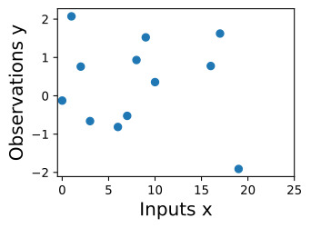
Suppose we observe the following dataset, of regression targets (outputs), y, indexed by inputs, x. As an example, the targets could be changes in carbon dioxide concentrations, and the inputs could be the times at which these targets have been recorded. What are some features of the data? How quickly does it seem to varying? Do we have data points collected at regular intervals, or are there missing inputs? How would you imagine filling in the missing regions, or forecasting up until x=25?
입력 x로 인덱싱된 회귀 목표(출력) y의 다음 데이터 세트를 관찰한다고 가정합니다. 예를 들어 목표는 이산화탄소 농도의 변화일 수 있고 입력은 이러한 목표가 기록된 시간일 수 있습니다. 데이터의 일부 기능은 무엇입니까? 얼마나 빨리 변하는 것 같나요? 정기적으로 수집된 데이터 포인트가 있습니까, 아니면 누락된 입력이 있습니까? 누락된 영역을 채우거나 x=25까지 예측하는 것을 어떻게 상상하시겠습니까?
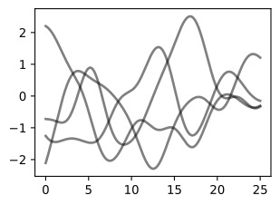
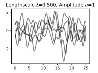
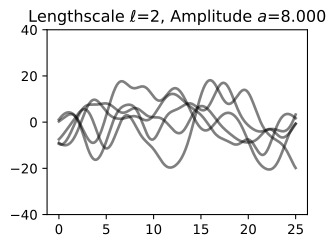
In order to fit the data with a Gaussian process, we start by specifying a prior distribution over what types of functions we might believe to be reasonable. Here we show several sample functions from a Gaussian process. Does this prior look reasonable? Note here we are not looking for functions that fit our dataset, but instead for specifying reasonable high-level properties of the solutions, such as how quickly they vary with inputs. Note that we will see code for reproducing all of the plots in this notebook, in the next notebooks on priors and inference.
데이터를 가우스 프로세스에 맞추려면 합리적이라고 믿을 수 있는 함수 유형에 대한 사전 분포를 지정하는 것부터 시작합니다. 여기서는 가우스 프로세스의 몇 가지 샘플 함수를 보여줍니다. 이 사전 조치가 합리적으로 보입니까? 여기서는 데이터 세트에 맞는 함수를 찾는 것이 아니라 입력에 따라 얼마나 빨리 변하는 지와 같은 솔루션의 합리적인 상위 수준 속성을 지정하기 위한 것입니다. 사전 및 추론에 대한 다음 노트북에서 이 노트북의 모든 플롯을 재현하기 위한 코드를 볼 수 있습니다.
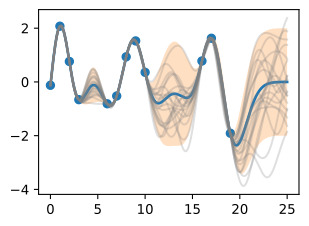
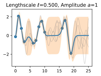
Once we condition on data, we can use this prior to infer a posterior distribution over functions that could fit the data. Here we show sample posterior functions.
데이터에 조건을 적용하면 데이터에 적합한 함수에 대한 사후 분포를 추론하기 전에 이를 사용할 수 있습니다. 여기서는 샘플 사후 함수를 보여줍니다.
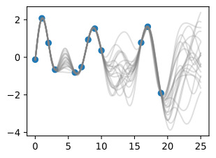
We see that each of these functions are entirely consistent with our data, perfectly running through each observation. In order to use these posterior samples to make predictions, we can average the values of every possible sample function from the posterior, to create the curve below, in thick blue. Note that we do not actually have to take an infinite number of samples to compute this expectation; as we will see later, we can compute the expectation in closed form.
우리는 이러한 각 함수가 데이터와 완전히 일치하며 각 관찰을 통해 완벽하게 실행된다는 것을 알 수 있습니다. 예측을 위해 이러한 사후 샘플을 사용하기 위해 사후에서 가능한 모든 샘플 함수의 값을 평균화하여 아래 곡선을 두꺼운 파란색으로 만들 수 있습니다. 이 기대치를 계산하기 위해 실제로 무한한 수의 샘플을 취할 필요는 없습니다. 나중에 살펴보겠지만 닫힌 형식으로 기대값을 계산할 수 있습니다.
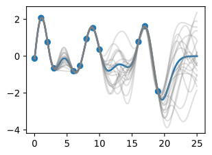
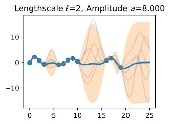
We may also want a representation of uncertainty, so we know how confident we should be in our predictions. Intuitively, we should have more uncertainty where there is more variability in the sample posterior functions, as this tells us there are many more possible values the true function could take. This type of uncertainty is called epistemic uncertainty, which is the reducible uncertainty associated with lack of information. As we acquire more data, this type of uncertainty disappears, as there will be increasingly fewer solutions consistent with what we observe. Like with the posterior mean, we can compute the posterior variance (the variability of these functions in the posterior) in closed form. With shade, we show two times the posterior standard deviation on either side of the mean, creating a credible interval that has a 95% probability of containing the true value of the function for any input x.
우리는 불확실성을 표현하기를 원할 수도 있으므로 예측에 얼마나 자신감을 가져야 하는지 알 수 있습니다. 직관적으로, 표본 사후 함수에 변동성이 더 많을수록 불확실성이 커집니다. 이는 실제 함수가 취할 수 있는 가능한 값이 더 많다는 것을 의미하기 때문입니다. 이러한 유형의 불확실성을 인식론적 불확실성이라고 하며, 이는 정보 부족과 관련된 환원 가능한 불확실성입니다. 더 많은 데이터를 수집할수록 우리가 관찰한 것과 일치하는 솔루션이 점점 줄어들기 때문에 이러한 유형의 불확실성은 사라집니다. 사후 평균과 마찬가지로 사후 분산(후방에서 이러한 함수의 변동성)을 닫힌 형식으로 계산할 수 있습니다. 음영을 사용하면 평균의 양쪽에 사후 표준 편차의 두 배를 표시하여 입력 x에 대한 함수의 실제 값을 포함할 확률이 95%인 신뢰할 수 있는 구간을 만듭니다.
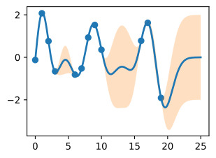
The plot looks somewhat cleaner if we remove the posterior samples, simply visualizing the data, posterior mean, and 95% credible set. Notice how the uncertainty grows away from the data, a property of epistemic uncertainty.
사후 샘플을 제거하고 데이터, 사후 평균 및 95% 신뢰 세트를 시각화하면 플롯이 다소 더 깨끗해 보입니다. 인식론적 불확실성의 속성인 불확실성이 데이터에서 어떻게 멀어지는지 주목하세요.
The properties of the Gaussian process that we used to fit the data are strongly controlled by what’s called a covariance function, also known as a kernel. The covariance function we used is called the RBF (Radial Basis Function) kernel, which has the form
데이터를 맞추는 데 사용한 가우스 프로세스의 속성은 커널이라고도 알려진 공분산 함수에 의해 강력하게 제어됩니다. 우리가 사용한 공분산 함수는 RBF(방사형 기초 함수) 커널이라고 하며 다음과 같은 형식을 갖습니다.

공분산 함수 (Covariance function) 란?
Covariance function (also known as a kernel function in machine learning) is a mathematical function used in statistics and machine learning to quantify the degree to which two random variables (or data points) vary together. It provides a measure of how correlated or related two variables are to each other.
공분산 함수 (머신 러닝에서는 커널 함수로도 알려져 있음)는 통계 및 머신 러닝에서 두 개의 랜덤 변수(또는 데이터 포인트)가 함께 얼마나 변하는지를 측정하는 수학적 함수입니다. 이것은 두 변수가 서로 어떻게 상관되거나 관련되어 있는지를 측정하는 데 사용됩니다.
In the context of statistics and Gaussian processes, the covariance function specifies the relationship between different points in a dataset. It defines how the value of one data point covaries or varies with the value of another data point. This information is crucial for modeling and understanding the underlying patterns and relationships within the data.
Covariance functions are often used in:
통계 및 가우시안 프로세스의 맥락에서 공분산 함수는 데이터 집합의 서로 다른 지점 간의 관계를 지정합니다. 이것은 하나의 데이터 포인트의 값이 다른 데이터 포인트의 값과 어떻게 공분산하거나 변하는지를 정의합니다. 이 정보는 데이터 내부의 기본적인 패턴과 관계를 모델링하고 이해하는 데 중요합니다.
공분산 함수는 다음과 같은 분야에서 사용됩니다.
- Gaussian Processes: In Gaussian processes, the covariance function (kernel) is a fundamental component. It determines how the values of the function being modeled vary across different input points. Common covariance functions include the Radial Basis Function (RBF) kernel, Matérn kernel, and many others.
가우시안 프로세스: 가우시안 프로세스에서 공분산 함수(커널)는 기본 구성 요소입니다. 이것은 모델링하려는 함수의 값이 다른 입력 지점에서 어떻게 변하는지를 결정합니다. 일반적인 공분산 함수에는 방사형 기저 함수(RBF) 커널, Matérn 커널 및 기타 여러 가지가 있습니다. - Spatial Statistics: In geostatistics and spatial statistics, covariance functions are used to model spatial dependencies in data, such as the correlation between temperatures at different locations on a map.
공간 통계: 지오통계 및 공간 통계에서 공분산 함수는 데이터 내에서 공간적 종속성(지도상의 다른 위치에서 온도 간의 상관 관계와 같은)을 모델링하는 데 사용됩니다. - Machine Learning: In machine learning, covariance functions are used in various algorithms, especially in kernel methods, including Support Vector Machines (SVMs) and Gaussian Process Regression (GPR).
머신 러닝: 머신 러닝에서 공분산 함수는 서포트 벡터 머신(SVM) 및 가우시안 프로세스 회귀(GPR)를 포함한 다양한 알고리즘에서 사용됩니다.
The choice of covariance function or kernel function has a significant impact on the performance of a model. Different covariance functions capture different types of relationships in the data, such as smoothness, periodicity, or linearity. Adjusting the parameters of the covariance function allows for fine-tuning the model's behavior.
공분산 함수 또는 커널 함수의 선택은 모델의 성능에 큰 영향을 미칩니다. 서로 다른 공분산 함수는 데이터에서 서로 다른 유형의 관계(부드러움, 주기성, 직선성 등)를 포착하며 공분산 함수의 매개변수를 조정하면 모델의 동작을 세밀하게 조정할 수 있습니다.
The hyperparameters of this kernel are interpretable. The amplitude parameter 'a' controls the vertical scale over which the function is varying, and the length-scale parameter ℓ controls the rate of variation (the wiggliness) of the function. Larger 'a' means larger function values, and larger ℓ means more slowly varying functions. Let’s see what happens to our sample prior and posterior functions as we vary 'a' and ℓ.
이 커널의 하이퍼파라미터는 해석 가능합니다. 진폭 매개변수 'a'는 함수가 변하는 수직 스케일을 제어하고, 길이 스케일 매개변수 ℓ는 함수의 변동률(흔들림)을 제어합니다. 'a'가 클수록 함수 값이 크고, ℓ가 클수록 함수가 천천히 변한다는 의미입니다. 'a'와 ℓ를 변경하면 샘플 사전 및 사후 함수에 어떤 일이 발생하는지 살펴보겠습니다.
The length-scale has a particularly pronounced effect on the predictions and uncertainty of a GP. At ||x−x′||=ℓ , the covariance between a pair of function values is a**2exp(−0.5). At larger distances than ℓ , the values of the function values becomes nearly uncorrelated. This means that if we want to make a prediction at a point x∗, then function values with inputs x such that ||x−x′||>ℓ will not have a strong effect on our predictions.
길이 척도는 GP의 예측과 불확실성에 특히 뚜렷한 영향을 미칩니다. ||x−x′||=ℓ 에서 함수 값 쌍 사이의 공분산은 a**2exp(−0.5)입니다. ℓ 보다 큰 거리에서는 함수 값의 상관관계가 거의 없어집니다. 이는 x* 지점에서 예측을 수행하려는 경우 ||x−x′||>ℓ와 같은 입력 x가 있는 함수 값이 예측에 큰 영향을 미치지 않음을 의미합니다.
Let’s see how changing the lengthscale affects sample prior and posterior functions, and credible sets. The above fits use a length-scale of 2. Let’s now consider ℓ=0.1,0.5,2,5,10 . A length-scale of 0.1 is very small relative to the range of the input domain we are considering, 25. For example, the values of the function at x=5 and x=10 will have essentially no correlation at such a length-scale. On the other hand, for a length-scale of 10, the function values at these inputs will be highly correlated. Note that the vertical scale changes in the following figures.
길이 척도를 변경하면 샘플 사전 및 사후 함수와 신뢰할 수 있는 세트에 어떤 영향을 미치는지 살펴보겠습니다. 위의 피팅은 길이 척도 2를 사용합니다. 이제 ℓ=0.1,0.5,2,5,10을 고려해 보겠습니다. 0.1의 길이 척도는 우리가 고려하고 있는 입력 영역의 범위인 25에 비해 매우 작습니다. 예를 들어 x=5와 x=10의 함수 값은 이러한 길이 척도에서 본질적으로 상관 관계가 없습니다. . 반면, 길이 척도가 10인 경우 이러한 입력의 함수 값은 높은 상관 관계를 갖습니다. 다음 그림에서는 수직 스케일이 변경됩니다.
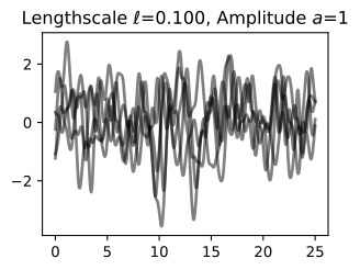
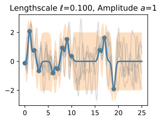

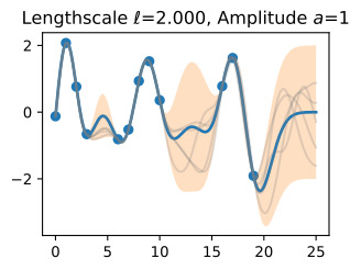
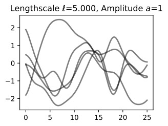
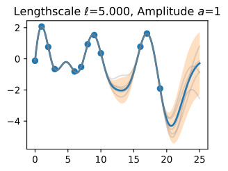
Notice as the length-scale increases the ‘wiggliness’ of the functions decrease, and our uncertainty decreases. If the length-scale is small, the uncertainty will quickly increase as we move away from the data, as the datapoints become less informative about the function values.
길이 척도가 증가함에 따라 함수의 '흔들림'이 감소하고 불확실성이 감소합니다. 길이 척도가 작으면 데이터 포인트가 함수 값에 대한 정보를 덜 제공하므로 데이터에서 멀어질수록 불확실성이 빠르게 증가합니다.
Now, let’s vary the amplitude parameter, holding the length-scale fixed at 2. Note the vertical scale is held fixed for the prior samples, and varies for the posterior samples, so you can clearly see both the increasing scale of the function, and the fits to the data.
이제 길이 스케일을 2로 고정하여 진폭 매개변수를 변경해 보겠습니다. 수직 스케일은 이전 샘플에 대해 고정되어 있고 사후 샘플에 대해 달라집니다. 따라서 함수의 스케일 증가와 데이터에 적합합니다.
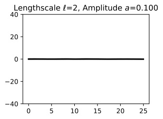
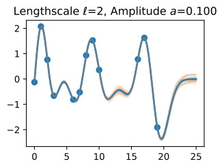

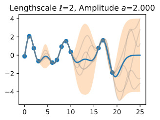
We see the amplitude parameter affects the scale of the function, but not the rate of variation. At this point, we also have the sense that the generalization performance of our procedure will depend on having reasonable values for these hyperparameters. Values of ℓ=2 and a=1 appeared to provide reasonable fits, while some of the other values did not. Fortunately, there is a robust and automatic way to specify these hyperparameters, using what is called the marginal likelihood, which we will return to in the notebook on inference.
진폭 매개변수는 함수의 규모에 영향을 주지만 변동률에는 영향을 미치지 않습니다. 이 시점에서 우리는 프로시저의 일반화 성능이 이러한 하이퍼파라미터에 대한 합리적인 값을 갖는지에 달려 있다는 것을 알게 되었습니다. ℓ=2 및 a=1 값은 합리적인 적합치를 제공하는 것으로 보였지만 일부 다른 값은 그렇지 않았습니다. 다행스럽게도 한계 우도(Marginal Likelihood)를 사용하여 이러한 하이퍼파라미터를 지정하는 강력하고 자동적인 방법이 있습니다. 이 방법은 추론에 대한 노트북에서 다시 설명하겠습니다.
So what is a GP, really? As we started, a GP simply says that any collection of function values f(x1),…,f(xn), indexed by any collection of inputs x1,…,xn has a joint multivariate Gaussian distribution. The mean vector μ of this distribution is given by a mean function, which is typically taken to be a constant or zero. The covariance matrix of this distribution is given by the kernel evaluated at all pairs of the inputs x.
그렇다면 GP란 무엇일까요? 우리가 시작했을 때, GP는 단순히 입력 x1,…,xn의 컬렉션에 의해 인덱스된 함수 값 f(x1),…,f(xn)의 컬렉션이 결합 다변량 가우스 분포를 갖는다고 말합니다. 이 분포의 평균 벡터 μ는 평균 함수로 제공되며 일반적으로 상수 또는 0으로 간주됩니다. 이 분포의 공분산 행렬은 모든 입력 x 쌍에서 평가된 커널에 의해 제공됩니다.
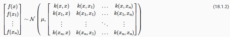
Equation (18.1.2) specifies a GP prior. We can compute the conditional distribution of f(x) for any x given f(x1),…,f(xn), the function values we have observed. This conditional distribution is called the posterior, and it is what we use to make predictions.
식 (18.1.2)은 GP 사전을 지정합니다. 우리가 관찰한 함수 값 f(x1),…,f(xn)이 주어지면 임의의 x에 대해 f(x)의 조건부 분포를 계산할 수 있습니다. 이 조건부 분포를 사후 분포라고 하며 예측을 위해 사용합니다.
In particular, 특히,
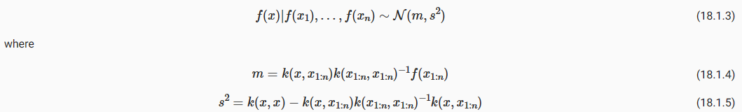
where k(x,x1:n) is a 1×n vector formed by evaluating k(x,xi) for i=1,…,n and k(x1:n,x1:n) is an n×n matrix formed by evaluating k(xi,xj) for i,j=1,…,n. m is what we can use as a point predictor for any x, and s**2 is what we use for uncertainty: if we want to create an interval with a 95% probability that f(x) is in the interval, we would use m±2s. The predictive means and uncertainties for all the above figures were created using these equations. The observed data points were given by f(x1),…,f(xn) and chose a fine grained set of x points to make predictions.
여기서 k(x,x1:n)은 i=1,…,n에 대해 k(x,xi)를 평가하여 형성된 1×n 벡터이고 k(x1:n,x1:n)은 형성된 n×n 행렬입니다. i,j=1,…,n에 대해 k(xi,xj)를 평가합니다. m은 임의의 x에 대한 점 예측자로 사용할 수 있는 것이고, s**2는 불확실성에 사용하는 것입니다. f(x)가 구간에 있을 확률이 95%인 구간을 생성하려면 다음과 같이 합니다. m±2초를 사용하세요. 위의 모든 수치에 대한 예측 평균과 불확실성은 이러한 방정식을 사용하여 생성되었습니다. 관찰된 데이터 포인트는 f(x1),…,f(xn)으로 제공되었으며 예측을 위해 세밀한 x 포인트 세트를 선택했습니다.
Let’s suppose we observe a single datapoint, f(x1), and we want to determine the value of f(x) at some x. Because f(x) is described by a Gaussian process, we know the joint distribution over (f(x),f(x1)) is Gaussian:
단일 데이터 포인트 f(x1)를 관찰하고 일부 x에서 f(x)의 값을 결정한다고 가정해 보겠습니다. f(x)는 가우스 프로세스로 설명되므로 (f(x),f(x1))에 대한 결합 분포가 가우스임을 알 수 있습니다.

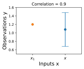
The off-diagonal expression k(x,x1)=k(x1,x) tells us how correlated the function values will be — how strongly determined f(x) will be from f(x1). We have seen already that if we use a large length-scale, relative to the distance between x and x1, ||x−x1||, then the function values will be highly correlated. We can visualize the process of determining f(x) from f(x1) both in the space of functions, and in the joint distribution over f(x1),f(x). Let’s initially consider an x such that k(x,x1)=0.9, and k(x,x)=1, meaning that the value of f(x) is moderately correlated with the value of f(x1). In the joint distribution, the contours of constant probability will be relatively narrow ellipses.
비대각선 표현식 k(x,x1)=k(x1,x)는 함수 값의 상관 관계, 즉 f(x)가 f(x1)에서 얼마나 강력하게 결정되는지 알려줍니다. 우리는 x와 x1 사이의 거리(||x−x1||)에 상대적으로 큰 길이 척도를 사용하면 함수 값의 상관 관계가 높다는 것을 이미 확인했습니다. 함수 공간과 f(x1),f(x)에 대한 결합 분포 모두에서 f(x1)에서 f(x)를 결정하는 프로세스를 시각화할 수 있습니다. 처음에 k(x,x1)=0.9, k(x,x)=1인 x를 고려해 보겠습니다. 이는 f(x) 값이 f(x1) 값과 중간 정도의 상관 관계가 있음을 의미합니다. 결합 분포에서 일정한 확률의 윤곽은 상대적으로 좁은 타원이 됩니다.
Suppose we observe f(x1)=1.2. To condition on this value of f(x1), we can draw a horizontal line at 1.2 on our plot of the density, and see that the value of f(x) is mostly constrained to [0.64,1.52]. We have also drawn this plot in function space, showing the observed point f(x1) in orange, and 1 standard deviation of the Gaussian process predictive distribution for f(x) in blue, about the mean value of 1.08.
f(x1)=1.2를 관찰한다고 가정합니다. 이 f(x1) 값을 조건으로 하기 위해 밀도 플롯에서 1.2에 수평선을 그릴 수 있으며 f(x) 값이 대부분 [0.64,1.52]로 제한되어 있음을 알 수 있습니다. 우리는 또한 이 플롯을 함수 공간에 그려서 관찰된 점 f(x1)을 주황색으로 표시하고 f(x)에 대한 가우스 프로세스 예측 분포의 1 표준 편차를 파란색으로 표시했습니다(평균값 약 1.08).

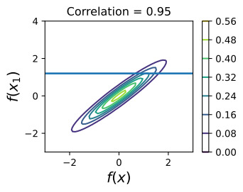
Now suppose we have a stronger correlation, k(x,x1)=0.95. Now the ellipses have narrowed further, and the value of f(x) is even more strongly determined by f(x1). Drawing a horizontal line at 1.2, we see the contours for f(x) support values mostly within [0.83,1.45]. Again, we also show the plot in function space, with one standard deviation about the mean predictive value of 1.14.
이제 k(x,x1)=0.95라는 더 강한 상관관계가 있다고 가정합니다. 이제 타원은 더 좁아졌고 f(x)의 값은 f(x1)에 의해 훨씬 더 강력하게 결정됩니다. 1.2에서 수평선을 그리면 f(x) 지원 값의 윤곽이 대부분 [0.83,1.45] 내에 있는 것을 볼 수 있습니다. 다시 말하지만, 평균 예측 값 1.14에 대한 표준 편차가 1인 함수 공간의 플롯도 표시됩니다.
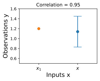
We see that the posterior mean predictor of our Gaussian process is closer to 1.2, because there is now a stronger correlation. We also see that our uncertainty (the error bars) have somewhat decreased. Despite the strong correlation between these function values, our uncertainty is still righly quite large, because we have only observed a single data point!
이제 더 강한 상관관계가 있기 때문에 가우스 프로세스의 사후 평균 예측 변수가 1.2에 더 가깝다는 것을 알 수 있습니다. 또한 불확실성(오차 막대)이 다소 감소한 것을 볼 수 있습니다. 이러한 함수 값 사이의 강한 상관 관계에도 불구하고 우리는 단 하나의 데이터 포인트만 관찰했기 때문에 불확실성은 여전히 상당히 큽니다!
This procedure can give us a posterior on f(x) for any x, for any number of points we have observed. Suppose we observe f(x1),f(x2). We now visualize the posterior for f(x) at a particular x=x′ in function space. The exact distribution for f(x) is given by the above equations. f(x) is Gaussian distributed, with mean
이 절차는 우리가 관찰한 임의의 수의 점에 대해 임의의 x에 대한 f(x)의 사후값을 제공할 수 있습니다. f(x1),f(x2)를 관찰한다고 가정합니다. 이제 함수 공간의 특정 x=x′에서 f(x)의 사후를 시각화합니다. f(x)의 정확한 분포는 위 방정식으로 제공됩니다. f(x)는 평균을 갖는 가우스 분포입니다.

and variance 및 분산

In this introductory notebook, we have been considering noise free observations. As we will see, it is easy to include observation noise. If we assume that the data are generated from a latent noise free function f(x) plus iid Gaussian noise ϵ(x)∼N(0,σ**2) with variance σ**2, then our covariance function simply becomes k(xi,xj)→k(xi,xj)+δijσ**2, where δif=1 if i=j and 0 otherwise.
이 소개 노트에서는 잡음 없는 관찰을 고려했습니다. 앞으로 살펴보겠지만 관찰 노이즈를 포함하는 것은 쉽습니다. 데이터가 잠재 잡음 없는 함수 f(x)와 분산 σ**2를 갖는 iid 가우스 잡음 ϵ(x)∼N(0,σ**2)에서 생성된다고 가정하면 공분산 함수는 간단히 k가 됩니다. (xi,xj)→k(xi,xj)+δijσ**2, 여기서 i=j이면 δif=1이고 그렇지 않으면 0입니다.
We have already started getting some intuition about how we can use a Gaussian process to specify a prior and posterior over solutions, and how the kernel function affects the properties of these solutions. In the following notebooks, we will precisely show how to specify a Gaussian process prior, introduce and derive various kernel functions, and then go through the mechanics of how to automatically learn kernel hyperparameters, and form a Gaussian process posterior to make predictions. While it takes time and practice to get used to concepts such as a “distributions over functions”, the actual mechanics of finding the GP predictive equations is actually quite simple — making it easy to get practice to form an intuitive understanding of these concepts.
우리는 이미 가우스 프로세스를 사용하여 솔루션에 대한 사전 및 사후를 지정하는 방법과 커널 기능이 이러한 솔루션의 속성에 어떻게 영향을 미치는지에 대한 직관을 얻기 시작했습니다. 다음 노트에서는 사전에 가우스 프로세스를 지정하는 방법, 다양한 커널 함수를 소개 및 도출하는 방법, 그리고 커널 하이퍼파라미터를 자동으로 학습하는 방법, 사후에 가우스 프로세스를 형성하여 예측하는 방법에 대한 메커니즘을 자세히 보여줍니다. "함수에 대한 분포"와 같은 개념에 익숙해지려면 시간과 연습이 필요하지만 GP 예측 방정식을 찾는 실제 메커니즘은 실제로 매우 간단하므로 이러한 개념을 직관적으로 이해하기 위한 연습을 쉽게 할 수 있습니다.
18.1.1. Summary
In typical machine learning, we specify a function with some free parameters (such as a neural network and its weights), and we focus on estimating those parameters, which may not be interpretable. With a Gaussian process, we instead reason about distributions over functions directly, which enables us to reason about the high-level properties of the solutions. These properties are controlled by a covariance function (kernel), which often has a few highly interpretable hyperparameters. These hyperparameters include the length-scale, which controls how rapidly (how wiggily) the functions are. Another hyperparameter is the amplitude, which controls the vertical scale over which our functions are varying. Representing many different functions that can fit the data, and combining them all together into a predictive distribution, is a distinctive feature of Bayesian methods. Because there is a greater amount of variability between possible solutions far away from the data, our uncertainty intuitively grows as we move from the data.
일반적인 기계 학습에서는 일부 자유 매개변수(예: 신경망 및 해당 가중치)를 사용하여 함수를 지정하고 해석할 수 없는 이러한 매개변수를 추정하는 데 중점을 둡니다. 가우스 프로세스를 사용하면 함수에 대한 분포를 직접 추론할 수 있으므로 솔루션의 상위 수준 속성을 추론할 수 있습니다. 이러한 속성은 해석 가능한 몇 가지 하이퍼 매개변수가 있는 공분산 함수(커널)에 의해 제어됩니다. 이러한 하이퍼파라미터에는 함수의 속도(얼마나 흔들리는지)를 제어하는 길이 척도가 포함됩니다. 또 다른 하이퍼파라미터는 진폭으로, 함수가 변하는 수직 스케일을 제어합니다. 데이터를 맞출 수 있는 다양한 함수를 표현하고 이를 모두 예측 분포로 결합하는 것은 베이지안 방법의 독특한 특징입니다. 데이터에서 멀리 떨어져 있는 가능한 솔루션 간에는 더 큰 변동성이 있기 때문에 데이터에서 이동할 때 불확실성이 직관적으로 커집니다.
A Gaussian process represents a distribution over functions by specifying a multivariate normal (Gaussian) distribution over all possible function values. It is possible to easily manipulate Gaussian distributions to find the distribution of one function value based on the values of any set of other values. In other words, if we observe a set of points, then we can condition on these points and infer a distribution over what the value of the function might look like at any other input. How we model the correlations between these points is determined by the covariance function and is what defines the generalization properties of the Gaussian process. While it takes time to get used to Gaussian processes, they are easy to work with, have many applications, and help us understand and develop other model classes, like neural networks.
가우스 프로세스는 가능한 모든 함수 값에 대해 다변량 정규(가우스) 분포를 지정하여 함수에 대한 분포를 나타냅니다. 가우스 분포를 쉽게 조작하여 다른 값 세트의 값을 기반으로 한 함수 값의 분포를 찾는 것이 가능합니다. 즉, 일련의 점을 관찰하면 이러한 점을 조건으로 하고 다른 입력에서 함수 값이 어떻게 보일지에 대한 분포를 추론할 수 있습니다. 이러한 점 간의 상관 관계를 모델링하는 방법은 공분산 함수에 의해 결정되며 이것이 가우스 프로세스의 일반화 속성을 정의합니다. 가우스 프로세스에 익숙해지는 데는 시간이 걸리지만 작업하기 쉽고 응용 프로그램이 많으며 신경망과 같은 다른 모델 클래스를 이해하고 개발하는 데 도움이 됩니다.
18.1.2. Exercises
- What is the difference between epistemic uncertainty versus observation uncertainty?
- Besides rate of variation and amplitude, what other properties of functions might we want to consider, and what would be real-world examples of functions that have those properties?
- The RBF covariance function we considered says that covariances (and correlations) between observations decrease with their distance in the input space (times, spatial locations, etc.). Is this a reasonable assumption? Why or why not?
- Is a sum of two Gaussian variables Gaussian? Is a product of two Gaussian variables Gaussian? If (a,b) have a joint Gaussian distribution, is a|b (a given b) Gaussian? Is a Gaussian?

6. Do you think increasing our estimate of observation noise would increase or decrease our estimate of the length-scale of the ground truth function?
7. As we move away from the data, suppose the uncertainty in our predictive distribution increases to a point, then stops increasing. Why might that happen?
'Dive into Deep Learning > D2L Gaussian Processes' 카테고리의 다른 글
| D2L - 18.3. Gaussian Process Inference (0) | 2023.09.10 |
|---|---|
| D2L - 18.2. Gaussian Process Priors (1) | 2023.09.09 |
| D2L - 18. Gaussian Processes (0) | 2023.09.09 |