5.7. Predicting House Prices on Kaggle — Dive into Deep Learning 1.0.0-beta0 documentation (d2l.ai)

5.7. Predicting House Prices on Kaggle

Now that we have introduced some basic tools for building and training deep networks and regularizing them with techniques including weight decay and dropout, we are ready to put all this knowledge into practice by participating in a Kaggle competition. The house price prediction competition is a great place to start. The data is fairly generic and do not exhibit exotic structure that might require specialized models (as audio or video might). This dataset, collected by De Cock (2011), covers house prices in Ames, IA from the period of 2006–2010. It is considerably larger than the famous Boston housing dataset of Harrison and Rubinfeld (1978), boasting both more examples and more features.

딥 네트워크를 구축 및 교육하고 가중치 감쇠 및 드롭아웃을 포함한 기술로 정규화하기 위한 몇 가지 기본 도구를 도입했으므로 Kaggle 경쟁에 참여하여 이 모든 지식을 실행할 준비가 되었습니다. 집값 예측 경쟁은 시작하기에 좋은 장소입니다. 데이터는 상당히 일반적이며 특수 모델(오디오 또는 비디오처럼)이 필요할 수 있는 이국적인 구조를 나타내지 않습니다. De Cock(2011)이 수집한 이 데이터 세트는 2006~2010년 기간 동안 아이오와 주 에임스의 주택 가격을 다룹니다. 이것은 Harrison과 Rubinfeld(1978)의 유명한 보스턴 주택 데이터 세트보다 상당히 크며 더 많은 예제와 더 많은 기능을 자랑합니다.

In this section, we will walk you through details of data preprocessing, model design, and hyperparameter selection. We hope that through a hands-on approach, you will gain some intuitions that will guide you in your career as a data scientist.

이 섹션에서는 데이터 전처리, 모델 설계 및 하이퍼파라미터 선택에 대한 세부 정보를 안내합니다. 실제 접근 방식을 통해 데이터 과학자로서의 경력을 안내할 몇 가지 직관을 얻을 수 있기를 바랍니다.

%matplotlib inline
import pandas as pd
import torch
from torch import nn
from d2l import torch as d2l

위 코드는 데이터 시각화 및 데이터 처리에 필요한 라이브러리를 가져오는 예시입니다.

• %matplotlib inline: 이 코드는 Jupyter Notebook 환경에서 matplotlib 그래프를 인라인으로 표시하도록 설정하는 명령입니다. 즉, 그래프를 코드 셀 아래에 바로 표시하도록 합니다.
• import pandas as pd: pandas는 데이터 분석과 조작에 유용한 라이브러리입니다. pd는 관례적으로 pandas를 축약형으로 사용하기 위해 사용되는 별칭(alias)입니다.
• import torch: PyTorch는 딥러닝 프레임워크로서 텐서(Tensor) 기반의 계산을 지원합니다. torch는 PyTorch 라이브러리를 임포트하는 명령입니다.
• from torch import nn: nn 모듈은 PyTorch에서 신경망 모델을 구축하기 위한 다양한 클래스와 함수를 제공합니다. torch에서 nn 모듈을 가져옵니다.
• from d2l import torch as d2l: d2l(torch)은 Dive into Deep Learning 책의 공식 코딩 스타일을 지원하는 라이브러리입니다. d2l은 관례적으로 d2l(torch)를 축약형으로 사용하기 위해 사용되는 별칭(alias)입니다.

5.7.1. Downloading Data

Throughout the book, we will train and test models on various downloaded datasets. Here, we implement two utility functions to download files and extract zip or tar files. Again, we defer their implementations into Section 23.7.

책 전반에 걸쳐 다운로드한 다양한 데이터 세트에서 모델을 훈련하고 테스트합니다. 여기서는 파일을 다운로드하고 zip 또는 tar 파일을 추출하는 두 가지 유틸리티 기능을 구현합니다. 다시 한 번 구현을 섹션 23.7로 연기합니다.

def download(url, folder, sha1_hash=None):
    """Download a file to folder and return the local filepath."""

def extract(filename, folder):
    """Extract a zip/tar file into folder."""

위 코드는 파일 다운로드와 압축 해제 기능을 수행하는 함수들입니다.

• download(url, folder, sha1_hash=None): 이 함수는 주어진 URL에서 파일을 다운로드하여 지정된 폴더에 저장하고 로컬 파일 경로를 반환합니다. url은 다운로드할 파일의 URL입니다. folder는 파일을 저장할 폴더 경로입니다. sha1_hash는 선택적으로 제공되는 SHA1 해시 값으로, 다운로드한 파일의 해시 값을 확인하여 파일의 무결성을 검사할 수 있습니다.
• extract(filename, folder): 이 함수는 주어진 파일 이름의 압축 파일을 특정 폴더에 압축 해제합니다. filename은 압축 해제할 파일의 이름 또는 경로입니다. folder는 압축 해제된 파일을 저장할 폴더 경로입니다. 이 함수는 다양한 형식의 압축 파일을 지원합니다(예: zip, tar 등).

5.7.2. Kaggle

Kaggle is a popular platform that hosts machine learning competitions. Each competition centers on a dataset and many are sponsored by stakeholders who offer prizes to the winning solutions. The platform helps users to interact via forums and shared code, fostering both collaboration and competition. While leaderboard chasing often spirals out of control, with researchers focusing myopically on preprocessing steps rather than asking fundamental questions, there is also tremendous value in the objectivity of a platform that facilitates direct quantitative comparisons among competing approaches as well as code sharing so that everyone can learn what did and did not work. If you want to participate in a Kaggle competition, you will first need to register for an account (see Fig. 5.7.1).

Kaggle은 기계 학습 대회를 주최하는 인기 있는 플랫폼입니다. 각 대회는 데이터 세트를 중심으로 하며 우승 솔루션에 상품을 제공하는 이해 관계자가 많은 대회를 후원합니다. 이 플랫폼은 사용자가 포럼 및 공유 코드를 통해 상호 작용하여 협업과 경쟁을 촉진하도록 돕습니다. 리더보드 추격은 종종 통제 불능 상태가 되지만 연구자들은 근본적인 질문을 하기보다 전처리 단계에 근시안적으로 초점을 맞춥니다. 또한 경쟁 접근 방식 간의 직접적인 정량적 비교와 모든 사람이 효과가 있었던 것과 그렇지 않은 것을 배우십시오. Kaggle 대회에 참가하려면 먼저 계정을 등록해야 합니다(그림 5.7.1 참조).

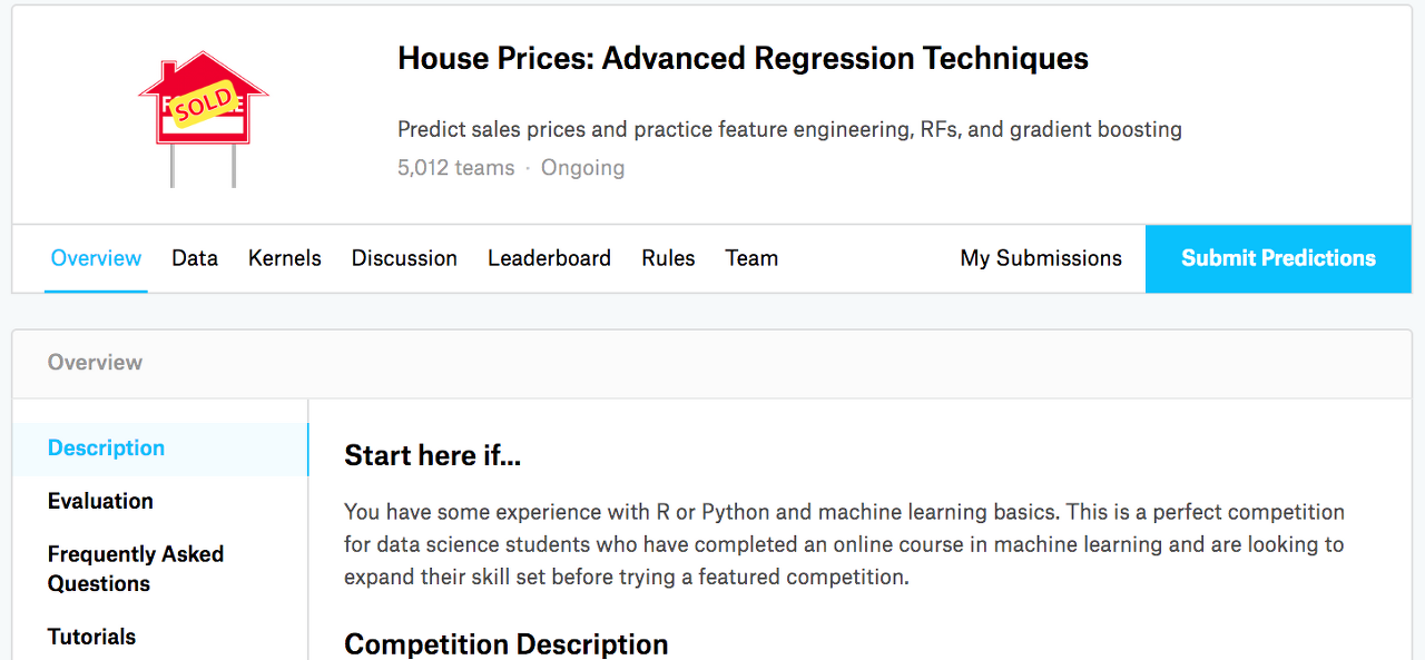
On the house price prediction competition page, as illustrated in Fig. 5.7.2, you can find the dataset (under the “Data” tab), submit predictions, and see your ranking, The URL is right here:

주택 가격 예측 경쟁 페이지에서 그림 5.7.2와 같이 데이터 세트("데이터" 탭 아래)를 찾고 예측을 제출하고 순위를 볼 수 있습니다. URL은 바로 여기에 있습니다.

https://www.kaggle.com/c/house-prices-advanced-regression-techniques

5.7.3. Accessing and Reading the Dataset

Note that the competition data is separated into training and test sets. Each record includes the property value of the house and attributes such as street type, year of construction, roof type, basement condition, etc. The features consist of various data types. For example, the year of construction is represented by an integer, the roof type by discrete categorical assignments, and other features by floating point numbers. And here is where reality complicates things: for some examples, some data is altogether missing with the missing value marked simply as “na”. The price of each house is included for the training set only (it is a competition after all). We will want to partition the training set to create a validation set, but we only get to evaluate our models on the official test set after uploading predictions to Kaggle. The “Data” tab on the competition tab in Fig. 5.7.2 has links to download the data.

competition 데이터는 훈련 및 테스트 세트로 구분됩니다. 각 레코드에는 집의 재산 가치와 거리 유형, 건축 연도, 지붕 유형, 지하실 상태 등과 같은 속성이 포함됩니다. 기능은 다양한 데이터 유형으로 구성됩니다. 예를 들어 건설 연도는 정수로, 지붕 유형은 불연속 범주 지정으로, 기타 기능은 부동 소수점 숫자로 표시됩니다. 그리고 여기에서 현실이 문제를 복잡하게 만듭니다. 일부 예의 경우 단순히 "na"로 표시된 누락된 값과 함께 일부 데이터가 완전히 누락되었습니다. 각 집의 가격은 훈련 세트에만 포함되어 있습니다 (결국 competition입니다). 훈련 세트를 분할하여 유효성 검사 세트를 만들고 싶지만 Kaggle에 예측을 업로드한 후에만 공식 테스트 세트에서 모델을 평가할 수 있습니다. 그림 5.7.2의 경쟁 탭에 있는 "데이터" 탭에는 데이터를 다운로드할 수 있는 링크가 있습니다.

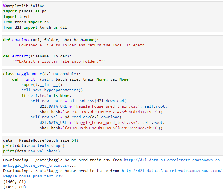
To get started, we will read in and process the data using pandas, which we have introduced in Section 2.2. For convenience, we can download and cache the Kaggle housing dataset. If a file corresponding to this dataset already exists in the cache directory and its SHA-1 matches sha1_hash, our code will use the cached file to avoid clogging up your internet with redundant downloads.

시작하려면 섹션 2.2에서 소개한 pandas를 사용하여 데이터를 읽고 처리합니다. 편의를 위해 Kaggle 주택 데이터 세트를 다운로드하고 캐시할 수 있습니다. 이 데이터 세트에 해당하는 파일이 이미 캐시 디렉터리에 있고 해당 SHA-1이 sha1_hash와 일치하는 경우 코드는 캐시된 파일을 사용하여 중복 다운로드로 인터넷이 막히는 것을 방지합니다.

class KaggleHouse(d2l.DataModule):
    def __init__(self, batch_size, train=None, val=None):
        super().__init__()
        self.save_hyperparameters()
        if self.train is None:
            self.raw_train = pd.read_csv(d2l.download(
                d2l.DATA_URL + 'kaggle_house_pred_train.csv', self.root,
                sha1_hash='585e9cc93e70b39160e7921475f9bcd7d31219ce'))
            self.raw_val = pd.read_csv(d2l.download(
                d2l.DATA_URL + 'kaggle_house_pred_test.csv', self.root,
                sha1_hash='fa19780a7b011d9b009e8bff8e99922a8ee2eb90'))

위 코드는 Kaggle House 데이터 세트를 처리하기 위한 데이터 모듈 클래스입니다.

• KaggleHouse 클래스는 d2l.DataModule 클래스를 상속합니다.
• __init__ 메서드에서는 batch_size, train, val 등의 매개변수를 받습니다.
• self.save_hyperparameters()를 호출하여 매개변수를 저장합니다.
• train이 None인 경우, pd.read_csv 함수를 사용하여 학습 데이터와 검증 데이터를 로드합니다.
• 학습 데이터는 Kaggle House 데이터 세트의 학습 세트(kaggle_house_pred_train.csv)로부터 로드합니다.
• 검증 데이터는 Kaggle House 데이터 세트의 테스트 세트(kaggle_house_pred_test.csv)로부터 로드합니다.
• 데이터를 로드하기 위해 d2l.download 함수를 사용하며, 데이터의 무결성을 검사하기 위해 SHA1 해시 값을 제공합니다.

The training dataset includes 1460 examples, 80 features, and 1 label, while the validation data contains 1459 examples and 80 features.

학습 데이터 세트에는 1460개의 예, 80개의 기능 및 1개의 레이블이 포함되어 있고 검증 데이터에는 1459개의 예 및 80개의 기능이 포함되어 있습니다.

data = KaggleHouse(batch_size=64)
print(data.raw_train.shape)
print(data.raw_val.shape)

위 코드는 KaggleHouse 데이터 모듈을 사용하여 데이터를 로드하고, 로드한 데이터의 크기를 출력하는 예시입니다.

• KaggleHouse 클래스의 인스턴스인 data를 생성합니다. 이때 batch_size를 64로 지정합니다.
• data.raw_train.shape를 호출하여 학습 데이터의 크기를 출력합니다. raw_train은 pd.read_csv를 통해 로드한 학습 데이터를 의미합니다. 출력 결과는 학습 데이터의 행(row)과 열(column)의 수입니다.
• data.raw_val.shape를 호출하여 검증 데이터의 크기를 출력합니다. raw_val은 pd.read_csv를 통해 로드한 검증 데이터를 의미합니다. 출력 결과는 검증 데이터의 행(row)과 열(column)의 수입니다.

5.7.4. Data Preprocessing

Let’s take a look at the first four and last two features as well as the label (SalePrice) from the first four examples.

처음 네 가지 예의 레이블(SalePrice)뿐만 아니라 처음 네 가지 기능과 마지막 두 가지 기능을 살펴보겠습니다.

print(data.raw_train.iloc[:4, [0, 1, 2, 3, -3, -2, -1]])

위 코드는 학습 데이터에서 앞부분 4개의 샘플의 특정 열(column)들을 선택하여 출력하는 예시입니다.

• data.raw_train은 로드한 학습 데이터를 나타냅니다.
• iloc[:4, [0, 1, 2, 3, -3, -2, -1]]는 학습 데이터의 첫 4개 행과 열 인덱스가 0, 1, 2, 3, -3, -2, -1인 열들을 선택하는 것을 의미합니다.
• 출력 결과는 선택한 열들로 이루어진 4개의 샘플을 표 형태로 출력합니다.

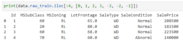
We can see that in each example, the first feature is the ID. This helps the model identify each training example. While this is convenient, it does not carry any information for prediction purposes. Hence, we will remove it from the dataset before feeding the data into the model. Besides, given a wide variety of data types, we will need to preprocess the data before we can start modeling.

각 예에서 첫 번째 feature가 ID임을 알 수 있습니다. 이렇게 하면 모델이 각 학습 예제를 식별하는 데 도움이 됩니다. 이는 편리하지만 예측 목적으로 어떤 정보도 전달하지 않습니다. 따라서 데이터를 모델에 공급하기 전에 데이터 세트에서 제거합니다. 게다가 다양한 데이터 유형이 주어지면 모델링을 시작하기 전에 데이터를 사전 처리해야 합니다.

Let’s start with the numerical features. First, we apply a heuristic, replacing all missing values by the corresponding feature’s mean. Then, to put all features on a common scale, we standardize the data by rescaling features to zero mean and unit variance:

numerical features부터 시작하겠습니다. 먼저 휴리스틱을 적용하여 누락된 모든 값을 해당 기능의 평균으로 바꿉니다. 그런 다음 모든 기능을 공통 척도에 놓기 위해 기능의 크기를 0 평균 및 단위 분산으로 재조정하여 데이터를 표준화합니다.

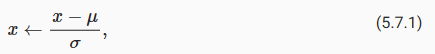
where μ and σ denote mean and standard deviation, respectively. To verify that this indeed transforms our feature (variable) such that it has zero mean and unit variance, note that E[x−μ/σ]=μ−μ/σ=0 and that E[(x−μ)²]=(σ²+μ²)−2μ²+μ²=σ². Intuitively, we standardize the data for two reasons. First, it proves convenient for optimization. Second, because we do not know a priori which features will be relevant, we do not want to penalize coefficients assigned to one feature more than on any other.

여기서 μ와 σ는 각각 평균과 표준 편차를 나타냅니다. 이것이 실제로 평균이 0이고 단위 분산이 있도록 특성(변수)을 변환하는지 확인하려면 E[x−μ/σ]=μ−μ/σ=0이고 E[(x−μ)2] =(σ2+μ2)-2μ2+μ2=σ2. 직관적으로 우리는 두 가지 이유로 데이터를 표준화합니다. 첫째, 최적화에 편리합니다. 둘째, 어떤 기능이 관련될지 선험적으로 알지 못하기 때문에 한 기능에 할당된 계수에 다른 기능보다 더 많은 페널티를 주고 싶지 않습니다.

Next we deal with discrete values. This includes features such as “MSZoning”. We replace them by a one-hot encoding in the same way that we previously transformed multiclass labels into vectors (see Section 4.1.1). For instance, “MSZoning” assumes the values “RL” and “RM”. Dropping the “MSZoning” feature, two new indicator features “MSZoning_RL” and “MSZoning_RM” are created with values being either 0 or 1. According to one-hot encoding, if the original value of “MSZoning” is “RL”, then “MSZoning_RL” is 1 and “MSZoning_RM” is 0. The pandas package does this automatically for us.

다음으로 이산 값을 다룹니다. 여기에는 "MSZoning"과 같은 기능이 포함됩니다. 이전에 다중 클래스 레이블을 벡터로 변환한 것과 동일한 방식으로 원-핫 인코딩으로 대체합니다(섹션 4.1.1 참조). 예를 들어 "MSZoning"은 "RL" 및 "RM" 값을 가정합니다. "MSZoning" 기능을 삭제하면 값이 0 또는 1인 두 개의 새로운 지표 기능인 "MSZoning_RL" 및 "MSZoning_RM"이 생성됩니다. 원-핫 인코딩에 따라 "MSZoning"의 원래 값이 "RL"이면 " MSZoning_RL”은 1이고 “MSZoning_RM”은 0입니다. pandas 패키지는 이를 자동으로 수행합니다.

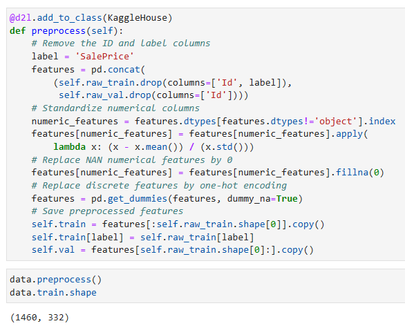
@d2l.add_to_class(KaggleHouse)
def preprocess(self):
    # Remove the ID and label columns
    label = 'SalePrice'
    features = pd.concat(
        (self.raw_train.drop(columns=['Id', label]),
         self.raw_val.drop(columns=['Id'])))
    # Standardize numerical columns
    numeric_features = features.dtypes[features.dtypes!='object'].index
    features[numeric_features] = features[numeric_features].apply(
        lambda x: (x - x.mean()) / (x.std()))
    # Replace NAN numerical features by 0
    features[numeric_features] = features[numeric_features].fillna(0)
    # Replace discrete features by one-hot encoding
    features = pd.get_dummies(features, dummy_na=True)
    # Save preprocessed features
    self.train = features[:self.raw_train.shape[0]].copy()
    self.train[label] = self.raw_train[label]
    self.val = features[self.raw_train.shape[0]:].copy()

위 코드는 KaggleHouse 클래스에 preprocess 메서드를 추가하는 예시입니다. preprocess 메서드는 데이터 전처리 과정을 수행합니다.

• self.raw_train은 원본 학습 데이터를 나타냅니다.
• self.raw_val은 원본 검증 데이터를 나타냅니다.

preprocess 메서드는 다음과 같은 과정을 거칩니다:

1. ID 열과 레이블 열(SalePrice)을 제외한 나머지 특성들을 features 변수에 결합합니다.
2. 숫자형 특성들을 표준화(Standardize)합니다. 숫자형 특성들은 features 변수에서 데이터 타입이 object가 아닌 열들을 선택하여 처리합니다. 각 숫자형 열의 값들을 해당 열의 평균과 표준편차를 이용하여 표준화합니다.
3. 결측값(NaN)이 있는 숫자형 특성들을 0으로 대체합니다.
4. 범주형 특성들을 원-핫 인코딩(one-hot encoding)합니다. dummy_na=True 옵션을 통해 결측값을 가진 특성도 처리합니다.
5. 전처리된 특성들을 self.train과 self.val에 저장합니다. self.train은 전처리된 학습 데이터를 나타내며, self.val은 전처리된 검증 데이터를 나타냅니다.

이를 통해 데이터 전처리가 수행되고, 최종적으로 전처리된 학습 데이터와 검증 데이터가 self.train과 self.val에 저장됩니다.

You can see that this conversion increases the number of features from 79 to 331 (excluding ID and label columns).

이 변환으로 features  수가 79개에서 331개로 증가하는 것을 볼 수 있습니다(ID 및 레이블 열 제외).

data.preprocess()
data.train.shape

위 코드는 data 객체에 대해 preprocess 메서드를 호출한 후에 data.train.shape를 출력하는 예시입니다.

data.preprocess()는 앞서 설명한 preprocess 메서드를 호출하여 데이터 전처리를 수행합니다. 전처리된 데이터는 self.train에 저장됩니다.

data.train.shape는 전처리된 학습 데이터의 크기(shape)를 나타냅니다. shape는 (행의 개수, 열의 개수) 형태로 반환되며, 이 코드에서는 전처리된 학습 데이터의 행의 개수를 나타냅니다. 따라서 위 코드는 전처리된 학습 데이터의 행의 개수를 출력합니다.

5.7.5. Error Measure

To get started we will train a linear model with squared loss. Not surprisingly, our linear model will not lead to a competition-winning submission but it provides a sanity check to see whether there is meaningful information in the data. If we cannot do better than random guessing here, then there might be a good chance that we have a data processing bug. And if things work, the linear model will serve as a baseline giving us some intuition about how close the simple model gets to the best reported models, giving us a sense of how much gain we should expect from fancier models.

시작하려면 제곱 손실(squared loss)이 있는 선형 모델을 훈련합니다. 당연히 우리의 선형 모델은 경쟁에서 우승하기 위해서 제출하는 것은 아닙니다.  데이터에 의미 있는 정보가 있는지 확인하기 위해 온전한 검사를 제공합니다. 여기서 우리가 무작위 추측(random guessing)보다 더 잘할 수 없다면 거기에는 데이터 처리 버그(data processing bug)가 있을 가능성이 높습니다. 그리고 제대로 작동한다면 선형 모델은 단순한 모델이 가장 잘 report된 모델에 얼마나 근접한지에 대한 직관을 제공하는 기준선 역할을 하여 더 멋진 모델에서 얼마나 많은 이득(gain )을 기대해야 하는지에 대한 감각을 제공합니다.

With house prices, as with stock prices, we care about relative quantities more than absolute quantities. Thus we tend to care more about the relative error y−y^/y than about the absolute error y−y^. For instance, if our prediction is off by USD 100,000 when estimating the price of a house in Rural Ohio, where the value of a typical house is 125,000 USD, then we are probably doing a horrible job. On the other hand, if we err by this amount in Los Altos Hills, California, this might represent a stunningly accurate prediction (there, the median house price exceeds 4 million USD).

주택 가격은 주식 가격과 마찬가지로 절대 수량보다 상대적 수량에 더 많은 관심을 기울입니다. 따라서 절대 오차 y−y^보다 상대 오차 y−y^/y에 더 신경을 쓰는 경향이 있습니다. 예를 들어, 일반적인 주택 가격이 125,000 USD인 시골 오하이오의 주택 가격을 추정할 때 예측이 USD 100,000만큼 빗나간다면 우리는 아마도 끔찍한 일을 하고 있는 것입니다. 반면에 캘리포니아의 로스 알토스 힐스에서 이 금액만큼 오류가 발생하면 놀라울 정도로 정확한 예측이 될 수 있습니다(거기 주택 중간 가격이 400만 달러를 초과함).

One way to address this problem is to measure the discrepancy in the logarithm of the price estimates. In fact, this is also the official error measure used by the competition to evaluate the quality of submissions. After all, a small value δ for |log⁡ y−log⁡ y^|≤δ translates into e^−δ≤y^/y≤e^δ. This leads to the following root-mean-squared-error between the logarithm of the predicted price and the logarithm of the label price:

@d2l.add_to_class(KaggleHouse)
def get_dataloader(self, train):
    label = 'SalePrice'
    data = self.train if train else self.val
    if label not in data: return
    get_tensor = lambda x: torch.tensor(x.values, dtype=torch.float32)
    # Logarithm of prices
    tensors = (get_tensor(data.drop(columns=[label])),  # X
               torch.log(get_tensor(data[label])).reshape((-1, 1)))  # Y
    return self.get_tensorloader(tensors, train)

위 코드는 get_dataloader라는 메서드를 KaggleHouse 클래스에 추가하는 예시입니다.

get_dataloader 메서드는 train 매개변수를 통해 학습 데이터 또는 검증 데이터에 대한 데이터 로더를 반환합니다. 메서드 내부에서는 label이라는 변수에 'SalePrice'를 할당하고, train이 True인 경우 self.train을 데이터로 선택하고, False인 경우 self.val을 데이터로 선택합니다.

그 후, get_tensor라는 람다 함수를 정의하여 데이터를 torch.tensor 형태로 변환합니다. get_tensor 함수는 데이터의 값을 torch.float32 자료형으로 변환하여 반환합니다.

마지막으로, tensors 변수에는 입력 데이터 X와 목표 데이터 Y가 포함된 튜플이 저장됩니다. X는 data에서 label 열을 제외한 값들을 torch.tensor로 변환한 것이고, Y는 data의 label 열을 로그 변환하여 torch.tensor로 변환한 것입니다. 이후, tensors를 이용하여 데이터 로더를 생성하고 반환합니다.

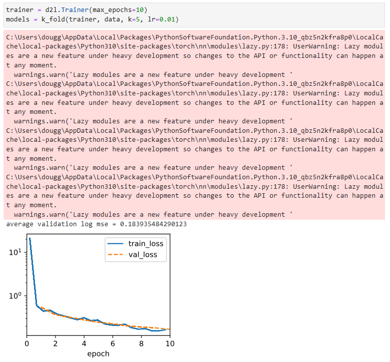
5.7.6. K-Fold Cross-Validation

You might recall that we introduced cross-validation in Section 3.6.3, where we discussed how to deal with model selection. We will put this to good use to select the model design and to adjust the hyperparameters. We first need a function that returns the i th fold of the data in a K-fold cross-validation procedure. It proceeds by slicing out the i th segment as validation data and returning the rest as training data. Note that this is not the most efficient way of handling data and we would definitely do something much smarter if our dataset was considerably larger. But this added complexity might obfuscate our code unnecessarily so we can safely omit it here owing to the simplicity of our problem.

모델 선택을 처리하는 방법에 대해 논의한 섹션 3.6.3에서 교차 검증을 소개한 것을 기억할 것입니다. 모델 설계를 선택하고 하이퍼파라미터를 조정하는 데 유용하게 사용할 것입니다. 먼저 K-폴드 교차 검증 절차에서 데이터의 i번째 폴드를 반환하는 함수가 필요합니다. i 번째 세그먼트를 유효성 검사 데이터로 잘라내고 나머지는 교육 데이터로 반환하는 방식으로 진행됩니다. 이것은 데이터를 처리하는 가장 효율적인 방법이 아니며 데이터 세트가 상당히 더 큰 경우 확실히 훨씬 더 스마트한 작업을 수행할 것입니다. 그러나이 추가 된 복잡성은 코드를 불필요하게 난독화할 수 있으므로 문제의 단순성으로 인해 여기에서 안전하게 생략할 수 있습니다.

def k_fold_data(data, k):
    rets = []
    fold_size = data.train.shape[0] // k
    for j in range(k):
        idx = range(j * fold_size, (j+1) * fold_size)
        rets.append(KaggleHouse(data.batch_size, data.train.drop(index=idx),
                                data.train.loc[idx]))
    return rets

위 코드는 k_fold_data라는 함수입니다. 이 함수는 데이터를 K-fold 교차 검증을 위해 K개의 폴드로 나누는 기능을 수행합니다.

k_fold_data 함수는 data와 k라는 두 개의 매개변수를 받습니다. 여기서 data는 KaggleHouse 클래스의 객체이며, k는 폴드의 개수를 나타냅니다.

함수 내부에서는 빈 리스트인 rets를 생성합니다. fold_size 변수에는 데이터의 학습 세트 크기를 K로 나눈 값이 저장됩니다. 그런 다음, range(k)를 반복하면서 폴드마다 인덱스를 생성합니다. 인덱스는 j * fold_size에서 (j+1) * fold_size까지의 범위로 생성됩니다.

마지막으로, rets 리스트에는 KaggleHouse 객체를 생성하여 추가합니다. 이때, 데이터의 배치 크기는 동일하게 유지되고, data.train에서 생성한 인덱스를 제외한 데이터를 학습 데이터로 사용하고, 해당 인덱스만을 가진 데이터를 검증 데이터로 사용합니다. 이 과정을 K번 반복하고, 최종적으로 rets 리스트에는 K개의 KaggleHouse 객체가 저장되어 반환됩니다.

The average validation error is returned when we train K times in the K-fold cross-validation.

K-겹 교차 검증에서 K번 훈련할 때 평균 검증 오류가 반환됩니다.

def k_fold(trainer, data, k, lr):
    val_loss, models = [], []
    for i, data_fold in enumerate(k_fold_data(data, k)):
        model = d2l.LinearRegression(lr)
        model.board.yscale='log'
        if i != 0: model.board.display = False
        trainer.fit(model, data_fold)
        val_loss.append(float(model.board.data['val_loss'][-1].y))
        models.append(model)
    print(f'average validation log mse = {sum(val_loss)/len(val_loss)}')
    return models

위 코드는 k_fold라는 함수입니다. 이 함수는 K-fold 교차 검증을 수행하여 모델을 학습하고, 각 폴드에서의 검증 손실과 학습된 모델을 반환합니다.

k_fold 함수는 trainer, data, k, lr 네 개의 매개변수를 받습니다. trainer는 학습을 담당하는 Trainer 객체, data는 KaggleHouse 객체, k는 폴드의 개수, lr은 학습률을 의미합니다.

함수 내부에서는 val_loss와 models라는 빈 리스트를 생성합니다. 이후, k_fold_data 함수를 호출하여 data 객체를 K개의 폴드로 나눕니다. 이때, 각 폴드마다 KaggleHouse 객체가 생성되고, data_fold에 저장됩니다.

그 다음, 반복문을 통해 각 폴드에 대해 모델을 학습합니다. 첫 번째 폴드에서는 model.board.display를 True로 설정하여 학습 과정을 출력하고, 이후 폴드에서는 출력을 생략하기 위해 model.board.display를 False로 설정합니다. trainer.fit 함수를 사용하여 모델을 학습하고, 검증 손실을 val_loss 리스트에 추가하고, 학습된 모델을 models 리스트에 추가합니다.

모든 폴드에 대한 학습이 완료되면, val_loss 리스트의 값들을 평균하여 평균 검증 손실을 출력합니다. 마지막으로, 학습된 모델들을 반환합니다.

5.7.7. Model Selection

In this example, we pick an untuned set of hyperparameters and leave it up to the reader to improve the model. Finding a good choice can take time, depending on how many variables one optimizes over. With a large enough dataset, and the normal sorts of hyperparameters, K-fold cross-validation tends to be reasonably resilient against multiple testing. However, if we try an unreasonably large number of options we might just get lucky and find that our validation performance is no longer representative of the true error.

이 예에서는 조정되지 않은 하이퍼파라미터 세트를 선택하고 모델을 개선하기 위해 독자에게 맡깁니다. 얼마나 많은 변수를 최적화하느냐에 따라 좋은 선택을 찾는 데 시간이 걸릴 수 있습니다. 충분히 큰 데이터 세트와 일반적인 종류의 하이퍼파라미터를 사용하면 K-겹 교차 검증은 여러 테스트에 대해 합리적으로 탄력적인 경향이 있습니다. 그러나 비합리적으로 많은 수의 옵션을 시도하면 운이 좋아 검증 성능이 더 이상 실제 오류를 나타내지 않는다는 것을 알게 될 수 있습니다.

trainer = d2l.Trainer(max_epochs=10)
models = k_fold(trainer, data, k=5, lr=0.01)

위 코드는 d2l.Trainer 객체를 생성하고, 이를 사용하여 k_fold 함수를 호출하는 부분입니다.

d2l.Trainer 객체는 학습을 관리하는 역할을 담당합니다. 생성자의 매개변수 max_epochs는 최대 학습 에포크 수를 나타내며, 이 경우 10으로 설정되어 있습니다.

k_fold 함수는 앞서 설명한 대로 K-fold 교차 검증을 수행하여 모델을 학습하고, 학습된 모델들을 반환합니다. 이때, trainer 객체를 첫 번째 매개변수로 전달하고, 두 번째 매개변수로는 데이터셋인 data 객체를 전달합니다. k는 폴드의 개수로 설정되어 있으며, lr은 학습률을 의미합니다.

models 변수는 k_fold 함수에서 반환된 학습된 모델들을 저장하는 리스트입니다.

* 로컬 결과

* 교재 결과

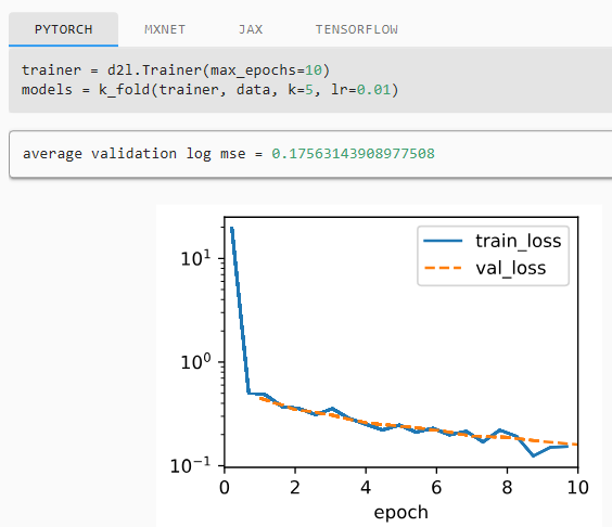
Notice that sometimes the number of training errors for a set of hyperparameters can be very low, even as the number of errors on K-fold cross-validation is considerably higher. This indicates that we are overfitting. Throughout training you will want to monitor both numbers. Less overfitting might indicate that our data can support a more powerful model. Massive overfitting might suggest that we can gain by incorporating regularization techniques.

K-겹 교차 검증의 오류 수가 상당히 높은 경우에도 하이퍼 매개변수 세트에 대한 훈련 오류 수가 때때로 매우 낮을 수 있다는 점에 유의하십시오. 이것은 우리가 과적합되고 있음을 나타냅니다. 교육 내내 두 숫자를 모두 모니터링하고 싶을 것입니다. 과적합이 적으면 데이터가 더 강력한 모델을 지원할 수 있음을 나타낼 수 있습니다. 대규모 과적합은 정규화 기술을 통합하여 얻을 수 있음을 시사할 수 있습니다.

5.7.8. Submitting Predictions on Kaggle

Now that we know what a good choice of hyperparameters should be, we might calculate the average predictions on the test set by all the K models. Saving the predictions in a csv file will simplify uploading the results to Kaggle. The following code will generate a file called submission.csv.

이제 우리는 하이퍼파라미터의 좋은 선택이 무엇인지 알았으므로 모든 K 모델에 의해 테스트 세트에 대한 평균 예측을 계산할 수 있습니다. csv 파일에 예측을 저장하면 결과를 Kaggle에 간단하게 업로드할 수 있습니다. 다음 코드는 submit.csv라는 파일을 생성합니다.

preds = [model(torch.tensor(data.val.values, dtype=torch.float32))
         for model in models]
# Taking exponentiation of predictions in the logarithm scale
ensemble_preds = torch.exp(torch.cat(preds, 1)).mean(1)
submission = pd.DataFrame({'Id':data.raw_val.Id,
                           'SalePrice':ensemble_preds.detach().numpy()})
submission.to_csv('submission.csv', index=False)

위 코드는 앙상블 모델을 사용하여 예측을 수행하고, 예측 결과를 제출용 CSV 파일로 저장하는 부분입니다.

preds는 앙상블에 사용할 모델들을 순회하면서 검증 데이터셋(data.val)에 대한 예측을 수행한 결과를 저장하는 리스트입니다. 예측 결과는 각 모델에 대해 torch.tensor를 사용하여 입력 데이터를 전달하여 계산되고, 이를 리스트에 추가합니다.

ensemble_preds는 preds 리스트에 저장된 예측 결과를 가지고 앙상블 예측을 수행한 결과입니다. 여기서는 예측 결과를 로그 스케일에서 다시 원래 스케일로 변환하기 위해 지수 함수(torch.exp)를 적용하고, torch.cat 함수를 사용하여 예측 결과를 열 방향으로 연결한 후 평균(mean(1))을 계산합니다. 최종 앙상블 예측은 평균값으로 구해집니다.

submission은 예측 결과를 저장하기 위한 DataFrame 객체입니다. data.raw_val.Id는 제출할 데이터의 ID 열을 나타내고, ensemble_preds.detach().numpy()는 앙상블 예측 결과를 넘파이 배열로 변환한 값으로 SalePrice 열을 나타냅니다.

마지막으로, submission을 CSV 파일로 저장하여 제출용 파일인 'submission.csv'로 저장합니다. index=False는 인덱스를 저장하지 않도록 설정하는 옵션입니다.

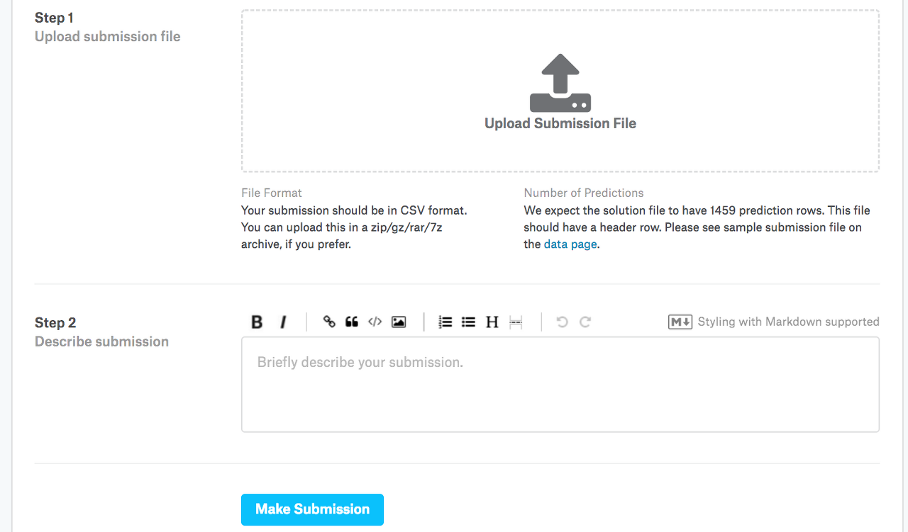
Next, as demonstrated in Fig. 5.7.3, we can submit our predictions on Kaggle and see how they compare with the actual house prices (labels) on the test set. The steps are quite simple:

다음으로 그림 5.7.3에 나와 있는 것처럼 Kaggle에 대한 예측을 제출하고 테스트 세트의 실제 주택 가격(라벨)과 비교하는 방법을 확인할 수 있습니다. 단계는 매우 간단합니다.

• Log in to the Kaggle website and visit the house price prediction competition page.
• Kaggle 웹 사이트에 로그인하고 집값 예측 경쟁 페이지를 방문하십시오.
• Click the “Submit Predictions” or “Late Submission” button (as of this writing, the button is located on the right).
• "예측 제출" 또는 "늦은 제출" 버튼을 클릭합니다(이 글을 쓰는 시점에서 버튼은 오른쪽에 있음).
• Click the “Upload Submission File” button in the dashed box at the bottom of the page and select the prediction file you wish to upload.
• 페이지 하단의 점선 상자에서 "제출 파일 업로드" 버튼을 클릭하고 업로드할 예측 파일을 선택합니다.
• Click the “Make Submission” button at the bottom of the page to view your results.
• 결과를 보려면 페이지 하단에 있는 "제출하기" 버튼을 클릭하십시오.

5.7.9. Summary

Real data often contains a mix of different data types and needs to be preprocessed. Rescaling real-valued data to zero mean and unit variance is a good default. So is replacing missing values with their mean. Besides, transforming categorical features into indicator features allows us to treat them like one-hot vectors. When we tend to care more about the relative error than about the absolute error, we can measure the discrepancy in the logarithm of the prediction. To select the model and adjust the hyperparameters, we can use K-fold cross-validation .

실제 데이터에는 다양한 데이터 유형이 혼합되어 있는 경우가 많으며 사전 처리가 필요합니다. 실수 값 데이터를 0 평균 및 단위 분산으로 재조정하는 것이 좋은 기본값입니다. 누락된 값을 평균으로 대체하는 것도 마찬가지입니다. 게다가 범주형 기능을 지표 기능으로 변환하면 원-핫 벡터처럼 처리할 수 있습니다. 절대 오차보다 상대 오차에 더 신경을 쓰는 경향이 있을 때 예측 로그의 불일치를 측정할 수 있습니다. 모델을 선택하고 하이퍼파라미터를 조정하기 위해 K-겹 교차 검증을 사용할 수 있습니다.

5.7.10. Exercises

1. Submit your predictions for this section to Kaggle. How good are your predictions?
2. Is it always a good idea to replace missing values by their mean? Hint: can you construct a situation where the values are not missing at random?
3. Improve the score on Kaggle by tuning the hyperparameters through K-fold cross-validation.
4. Improve the score by improving the model (e.g., layers, weight decay, and dropout).
5. What happens if we do not standardize the continuous numerical features like what we have done in this section?

5.6. Dropout — Dive into Deep Learning 1.0.0-beta0 documentation (d2l.ai)

5.6. Dropout

Let’s think briefly about what we expect from a good predictive model. We want it to peform well on unseen data. Classical generalization theory suggests that to close the gap between train and test performance, we should aim for a simple model. Simplicity can come in the form of a small number of dimensions. We explored this when discussing the monomial basis functions of linear models in Section 3.6. Additionally, as we saw when discussing weight decay (ℓ2 regularization) in Section 3.7, the (inverse) norm of the parameters also represents a useful measure of simplicity. Another useful notion of simplicity is smoothness, i.e., that the function should not be sensitive to small changes to its inputs. For instance, when we classify images, we would expect that adding some random noise to the pixels should be mostly harmless.

좋은 예측 모델에서 기대하는 바에 대해 간단히 생각해 봅시다. 우리는 그것이 보이지 않는 데이터에서 잘 작동하기를 원합니다. 고전적 일반화 이론은 학습과 테스트 성능 사이의 격차를 좁히기 위해 간단한 모델을 목표로 해야 한다고 제안합니다. 단순성은 차원 수가 적다는 형태로 나타날 수 있습니다. 우리는 섹션 3.6에서 선형 모델의 단항 기저 함수를 논의할 때 이것을 탐구했습니다. 또한 섹션 3.7에서 가중치 감쇠(ℓ2 정규화)를 논의할 때 보았듯이 매개변수의 (역) 규범도 단순성의 유용한 척도를 나타냅니다. 단순함의 또 다른 유용한 개념은 매끄러움입니다. 즉, 함수는 입력의 작은 변화에 민감하지 않아야 합니다. 예를 들어 이미지를 분류할 때 픽셀에 임의의 노이즈를 추가해도 대부분 무해할 것으로 예상합니다.

In 1995, Christopher Bishop formalized this idea when he proved that training with input noise is equivalent to Tikhonov regularization (Bishop, 1995). This work drew a clear mathematical connection between the requirement that a function be smooth (and thus simple), and the requirement that it be resilient to perturbations in the input.

1995년 Christopher Bishop은 입력 노이즈를 사용한 훈련이 Tikhonov 정규화와 동일하다는 것을 증명하면서 이 아이디어를 공식화했습니다(Bishop, 1995). 이 작업은 함수가 매끄럽고(따라서 단순해야 함) 요구 사항과 입력의 섭동(perturbations, 혼란, 동요, 당황)에 탄력적이어야 한다는 요구 사항 사이에 명확한 수학적 연결을 그렸습니다.

Then, in 2014, Srivastava et al. (2014) developed a clever idea for how to apply Bishop’s idea to the internal layers of a network, too. Their idea, called dropout, involves injecting noise while computing each internal layer during forward propagation, and it has become a standard technique for training neural networks. The method is called dropout because we literally drop out some neurons during training. Throughout training, on each iteration, standard dropout consists of zeroing out some fraction of the nodes in each layer before calculating the subsequent layer.

그런 다음 2014년 Srivastava et al. (2014)는 Bishop의 아이디어를 네트워크의 내부 계층에도 적용하는 방법에 대한 기발한 아이디어를 개발했습니다. 드롭아웃(dropout)이라고 하는 그들의 아이디어는 정방향 전파(forward propagation) 동안 각 내부 레이어를 계산하는 동안 노이즈를 주입하는 것과 관련이 있으며, 신경망 훈련을 위한 표준 기술이 되었습니다. 이 방법을 드롭아웃이라고 부르는 이유는 말 그대로 훈련 중에 일부 뉴런을 드롭아웃하기 때문입니다. 교육 전반에 걸쳐 각 반복에서 표준 드롭아웃은 후속 계층을 계산하기 전에 각 계층의 노드 일부를 0으로 만드는 것으로 구성됩니다.

Dropout이란?

Dropout is a regularization technique commonly used in machine learning, particularly in neural networks, to prevent overfitting and improve generalization performance. It involves randomly dropping out (setting to zero) a proportion of the neurons or connections in a neural network during training.

Dropout은 머신 러닝에서 흔히 사용되는 정규화 기법으로, 특히 신경망에서 과적합을 방지하고 일반화 성능을 향상시키는 데 사용됩니다. 학습 중에 신경망의 일부 뉴런이나 연결을 무작위로 비활성화(0으로 설정)하는 것이 특징입니다.

During each training iteration, dropout randomly masks (sets to zero) a certain fraction of the neurons or connections in a layer, effectively removing them from the network temporarily. This forces the network to learn with a reduced set of neurons and prevents individual neurons from relying too heavily on specific features or co-adapting with other neurons.

각 학습 반복에서 Dropout은 무작위로 일부 뉴런이나 연결을 마스킹하여 (0으로 설정하여) 신경망에서 임시로 제거합니다. 이렇게 함으로써 신경망은 줄어든 뉴런 집합을 사용하여 학습하게 되며, 개별 뉴런이 특정 특징에 지나치게 의존하거나 다른 뉴런과 공동으로 적응하는 것을 방지합니다.

By randomly dropping out neurons, dropout introduces noise and prevents the neural network from relying too heavily on any particular subset of neurons. This encourages the network to learn more robust and generalizable representations of the data.

Dropout은 무작위로 뉴런을 제거함으로써 노이즈를 도입하고, 신경망이 특정 뉴런 집합에 지나치게 의존하지 않도록 합니다. 이는 신경망이 더 견고하고 일반화 가능한 데이터 표현을 학습하도록 장려합니다.

During inference or testing, dropout is typically turned off, and the full network is used for making predictions.

추론이나 테스트 단계에서는 일반적으로 Dropout을 끄고 전체 네트워크를 사용하여 예측을 수행합니다.

To be clear, we are imposing our own narrative with the link to Bishop. The original paper on dropout offers intuition through a surprising analogy to sexual reproduction. The authors argue that neural network overfitting is characterized by a state in which each layer relies on a specific pattern of activations in the previous layer, calling this condition co-adaptation. dropout, they claim, breaks up co-adaptation just as sexual reproduction is argued to break up co-adapted genes. While the explanatory of this theory is certainly up for debate, the dropout technique itself has proved enduring, and various forms of dropout are implemented in most deep learning libraries.

명확히 하기 위해 우리는 Bishop에 대한 링크로 우리 자신의 내러티브를 부과하고 있습니다. dropout 에 관한 원본 논문은 유성 생식에 대한 놀라운 비유를 통해 직관을 제공합니다. 저자는 신경망 과적합이 각 계층이 이전 계층의 특정 활성화 패턴에 의존하는 상태를 특징으로 하며 이 조건을 공동 적응(co-adaptation)이라고 합니다. 그들은 유성 생식이 공동 적응된 유전자를 분열시킨다고 주장하듯이 중퇴는 공동 적응을 분열시킨다고 주장한다. 이 이론에 대한 설명은 확실히 논쟁의 여지가 있지만 드롭아웃 기술 자체는 오래 지속되는 것으로 입증되었으며 다양한 형태의 드롭아웃이 대부분의 딥 러닝 라이브러리에서 구현됩니다.

The key challenge is how to inject this noise. One idea is to inject the noise in an unbiased manner so that the expected value of each layer—while fixing the others—equals to the value it would have taken absent noise. In Bishop’s work, he added Gaussian noise to the inputs to a linear model. At each training iteration, he added noise sampled from a distribution with mean zero ϵ∼N(0,σ2) to the input x, yielding a perturbed point x′=x+ϵ. In expectation, E[x′]=x.

핵심 과제는 이 노이즈를 주입하는 방법입니다. 한 가지 아이디어는 편향되지 않은 방식으로 노이즈를 주입하여 각 레이어의 예상 값이 다른 레이어를 수정하는 동안 노이즈가 없는 값과 같도록 하는 것입니다. Bishop의 작업에서 그는 선형 모델의 입력에 가우시안 노이즈를 추가했습니다. 각 훈련 반복에서 그는 평균 0 ϵ~N(0,σ2)인 분포에서 샘플링된 노이즈를 입력 x에 추가하여 교란된 점 x′=x+ϵ를 산출했습니다. 예상대로 E[x′]=x.

In standard dropout regularization, one zeros out some fraction of the nodes in each layer and then debiases each layer by normalizing by the fraction of nodes that were retained (not dropped out). In other words, with dropout probability p, each intermediate activation ℎ is replaced by a random variable ℎ′ as follows:

표준 드롭아웃 정규화에서는 각 레이어의 일부 노드를 0으로 만든 다음 유지된(드롭아웃이 아닌) 노드의 일부로 정규화하여 각 레이어의 편향성을 제거합니다. 즉, 드롭아웃 확률이 p인 경우 각 중간 활성화 ℎ는 다음과 같이 임의 변수 ℎ'로 대체됩니다.

By design, the expectation remains unchanged, i.e., E[ℎ′]=ℎ.

설계상 기대치는 변하지 않습니다. 즉, E[ℎ′]=ℎ입니다.

import torch
from torch import nn
from d2l import torch as d2l

위 코드는 torch, torch.nn, 그리고 d2l 패키지를 임포트하는 예시입니다.

• torch: PyTorch의 기본 패키지로, 다양한 텐서 연산과 딥러닝 모델 구성을 위한 도구들을 제공합니다.
• torch.nn: PyTorch의 신경망 관련 모듈을 포함한 패키지로, 신경망 레이어, 활성화 함수, 손실 함수 등을 정의하고 제공합니다.
• d2l.torch: d2l 패키지에서 제공하는 PyTorch 관련 유틸리티 함수와 클래스들을 포함한 모듈입니다. 이 모듈은 d2l 패키지의 torch 모듈에 대한 별칭(Alias)로 사용됩니다.

해당 코드에서는 이러한 패키지와 모듈을 임포트하여 사용할 준비를 하고 있습니다. 이후 코드에서는 해당 패키지와 모듈의 함수와 클래스를 사용하여 신경망 모델을 정의하고 학습하는 등의 작업을 수행할 수 있습니다.

5.6.1. Dropout in Practice

Recall the MLP with a hidden layer and 5 hidden units in Fig. 5.1.1. When we apply dropout to a hidden layer, zeroing out each hidden unit with probability p, the result can be viewed as a network containing only a subset of the original neurons. In Fig. 5.6.1, ℎ2 and ℎ5 are removed. Consequently, the calculation of the outputs no longer depends on ℎ2 or ℎ5 and their respective gradient also vanishes when performing backpropagation. In this way, the calculation of the output layer cannot be overly dependent on any one element of ℎ1,…,ℎ5.

그림 5.1.1에서 은닉층과 5개의 은닉 유닛이 있는 MLP를 상기하십시오. 은닉층에 드롭아웃을 적용하여 각 은닉 유닛을 확률 p로 제로화하면 결과는 원래 뉴런의 하위 집합만 포함하는 네트워크로 볼 수 있습니다. 그림 5.6.1에서 ℎ2와 ℎ5는 제거되었다. 결과적으로 출력 계산은 더 이상 ℎ2 또는 ℎ5에 의존하지 않으며 역전파를 수행할 때 각 기울기도 사라집니다. 이와 같이 출력 레이어의 계산은 ℎ1,…,ℎ5 중 어느 하나의 요소에 지나치게 의존할 수 없습니다.

Typically, we disable dropout at test time. Given a trained model and a new example, we do not drop out any nodes and thus do not need to normalize. However, there are some exceptions: some researchers use dropout at test time as a heuristic for estimating the uncertainty of neural network predictions: if the predictions agree across many different dropout masks, then we might say that the network is more confident.

일반적으로 테스트 시 드롭아웃을 비활성화합니다. 훈련된 모델과 새 예제가 주어지면 노드를 삭제하지 않으므로 정규화할 필요가 없습니다. 그러나 몇 가지 예외가 있습니다. 일부 연구원은 신경망 예측의 불확실성을 추정하기 위한 휴리스틱으로 테스트 시간에 드롭아웃을 사용합니다. 여러 다른 드롭아웃 마스크에서 예측이 일치하면 네트워크가 더 확실하다고 말할 수 있습니다.

5.6.2. Implementation from Scratch

To implement the dropout function for a single layer, we must draw as many samples from a Bernoulli (binary) random variable as our layer has dimensions, where the random variable takes value 1 (keep) with probability 1−p and 0 (drop) with probability p. One easy way to implement this is to first draw samples from the uniform distribution U[0,1]. Then we can keep those nodes for which the corresponding sample is greater than p, dropping the rest.

단일 레이어에 대한 드롭아웃 기능을 구현하려면 레이어가 갖는 차원만큼 Bernoulli(이진) 랜덤 변수에서 많은 샘플을 가져와야 합니다. 여기서 랜덤 변수는 확률 1-p 및 0(드롭)으로 값 1(유지)을 취합니다. 확률로 p. 이를 구현하는 한 가지 쉬운 방법은 균일 분포 U[0,1]에서 먼저 샘플을 추출하는 것입니다. 그런 다음 해당 샘플이 p보다 큰 노드를 유지하고 나머지는 삭제할 수 있습니다.

In the following code, we implement a dropout_layer function that drops out the elements in the tensor input X with probability dropout, rescaling the remainder as described above: dividing the survivors by 1.0-dropout.

다음 코드에서는 텐서 입력 X의 요소를 드롭아웃 확률로 드롭아웃하는 dropout_layer 함수를 구현하고 나머지는 위에서 설명한 대로 생존자를 1.0-드롭아웃으로 나눕니다.

def dropout_layer(X, dropout):
    assert 0 <= dropout <= 1
    if dropout == 1: return torch.zeros_like(X)
    mask = (torch.rand(X.shape) > dropout).float()
    return mask * X / (1.0 - dropout)

위 코드는 드롭아웃(Dropout) 레이어를 구현한 함수입니다.

드롭아웃은 신경망에서 과적합을 방지하기 위해 사용되는 정규화 기법 중 하나로, 학습 중에 일부 뉴런을 임시로 제거하여 모델의 일반화 성능을 향상시키는 역할을 합니다.

이 함수는 입력인 X와 드롭아웃 확률인 dropout을 받습니다. dropout은 0과 1 사이의 값이어야 합니다. 만약 dropout이 1이라면 모든 뉴런을 제거하고 0으로 채운 텐서를 반환합니다. 그렇지 않은 경우에는 X와 같은 크기의 마스크를 생성하여 드롭아웃을 적용합니다.

마스크는 X와 같은 크기의 텐서를 생성하고, 각 요소가 dropout보다 큰 경우에는 1로 설정하고 dropout보다 작은 경우에는 0으로 설정합니다. 이렇게 함으로써 dropout 확률에 따라 일부 뉴런이 제거되는 효과를 얻을 수 있습니다.

마스크를 X와 곱한 뒤 dropout에 대한 보정을 수행하여 드롭아웃된 결과를 반환합니다. 보정은 마스크를 dropout의 보정값인 1/(1 - dropout)으로 나누어 줌으로써 드롭아웃이 적용된 값을 보정하는 역할을 합니다.

이렇게 구현된 dropout_layer 함수는 드롭아웃이 적용된 X를 반환합니다.

We can test out the dropout_layer function on a few examples. In the following lines of code, we pass our input X through the dropout operation, with probabilities 0, 0.5, and 1, respectively.

몇 가지 예에서 dropout_layer 함수를 테스트할 수 있습니다. 다음 코드 줄에서는 각각 확률 0, 0.5 및 1로 드롭아웃 작업을 통해 입력 X를 전달합니다.

X = torch.arange(16, dtype = torch.float32).reshape((2, 8))
print('dropout_p = 0:', dropout_layer(X, 0))
print('dropout_p = 0.5:', dropout_layer(X, 0.5))
print('dropout_p = 1:', dropout_layer(X, 1))

위 코드는 주어진 입력 X에 대해 dropout_layer 함수를 적용하여 드롭아웃된 결과를 출력하는 예시입니다.

입력 X는 크기가 (2, 8)인 2차원 텐서로, 각 원소는 0부터 15까지의 값으로 초기화되어 있습니다.

첫 번째 출력은 dropout_p가 0인 경우입니다. 즉, 드롭아웃 확률이 0이므로 모든 원소를 유지합니다. 따라서 출력은 입력 X와 동일한 텐서입니다.

두 번째 출력은 dropout_p가 0.5인 경우입니다. 드롭아웃 확률이 0.5이므로 각 원소가 0.5의 확률로 제거됩니다. 따라서 출력은 입력 X와 같은 크기의 텐서이지만, 일부 원소가 0으로 바뀌어 있습니다.

세 번째 출력은 dropout_p가 1인 경우입니다. 드롭아웃 확률이 1이므로 모든 원소가 제거되고 0으로 채워진 텐서가 반환됩니다.

이를 통해 드롭아웃 확률에 따라 일부 뉴런이 제거되는 효과를 확인할 수 있습니다.

5.6.2.1. Defining the Model

The model below applies dropout to the output of each hidden layer (following the activation function). We can set dropout probabilities for each layer separately. A common trend is to set a lower dropout probability closer to the input layer. We ensure that dropout is only active during training.

아래 모델은 각 숨겨진 레이어의 출력에 드롭아웃을 적용합니다(활성화 함수에 따름). 각 레이어에 대해 개별적으로 드롭아웃 확률을 설정할 수 있습니다. 일반적인 추세는 드롭아웃 확률을 입력 레이어에 더 가깝게 설정하는 것입니다. 교육 중에만 드롭아웃이 활성화되도록 합니다.

class DropoutMLPScratch(d2l.Classifier):
    def __init__(self, num_outputs, num_hiddens_1, num_hiddens_2,
                 dropout_1, dropout_2, lr):
        super().__init__()
        self.save_hyperparameters()
        self.lin1 = nn.LazyLinear(num_hiddens_1)
        self.lin2 = nn.LazyLinear(num_hiddens_2)
        self.lin3 = nn.LazyLinear(num_outputs)
        self.relu = nn.ReLU()

    def forward(self, X):
        H1 = self.relu(self.lin1(X.reshape((X.shape[0], -1))))
        if self.training:
            H1 = dropout_layer(H1, self.dropout_1)
        H2 = self.relu(self.lin2(H1))
        if self.training:
            H2 = dropout_layer(H2, self.dropout_2)
        return self.lin3(H2)

위 코드는 Dropout을 적용한 MLPScratch 모델 클래스를 정의하는 예시입니다.

이 모델은 입력 X를 받아 여러 개의 선형 레이어와 ReLU 활성화 함수를 거쳐 최종 출력을 생성합니다. 중간 레이어의 출력에는 Dropout이 적용됩니다.

• self.lin1, self.lin2, self.lin3: 선형 레이어 객체로, 입력과 출력의 차원을 매개변수로 설정하여 초기화됩니다.
• self.relu: ReLU 활성화 함수 객체로, ReLU 함수를 적용하기 위해 사용됩니다.

forward 메서드에서는 다음과 같은 과정을 거쳐 입력을 처리합니다:

1. 입력 X를 2차원으로 재구성합니다. 입력의 첫 번째 차원은 배치 크기를 의미합니다.
2. self.lin1을 통과한 결과에 ReLU 활성화 함수를 적용하여 H1을 얻습니다. 이때, 모델이 학습 중인 경우에만 Dropout이 적용됩니다.
3. self.lin2를 통과한 결과에 ReLU 활성화 함수를 적용하여 H2를 얻습니다. 마찬가지로, 모델이 학습 중인 경우에만 Dropout이 적용됩니다.
4. self.lin3을 통과한 결과를 반환합니다.

이를 통해 Dropout을 적용한 다층 퍼셉트론 모델의 순전파 과정을 구현하였습니다.

5.6.2.2. Training

The following is similar to the training of MLPs described previously.

다음은 앞에서 설명한 MLP 교육과 유사합니다.

hparams = {'num_outputs':10, 'num_hiddens_1':256, 'num_hiddens_2':256,
           'dropout_1':0.5, 'dropout_2':0.5, 'lr':0.1}
model = DropoutMLPScratch(**hparams)
data = d2l.FashionMNIST(batch_size=256)
trainer = d2l.Trainer(max_epochs=10)
trainer.fit(model, data)

위 코드는 Dropout을 적용한 MLPScratch 모델을 생성하고 학습하는 예시입니다.

• hparams: 모델의 하이퍼파라미터를 저장한 딕셔너리입니다. 'num_outputs', 'num_hiddens_1', 'num_hiddens_2', 'dropout_1', 'dropout_2', 'lr' 키를 갖고 각각 출력 개수, 첫 번째 은닉층 크기, 두 번째 은닉층 크기, 첫 번째 Dropout 비율, 두 번째 Dropout 비율, 학습률을 값으로 갖습니다.
• model: DropoutMLPScratch 클래스의 인스턴스로, 앞서 정의한 하이퍼파라미터를 인자로 넘겨 생성됩니다.
• data: d2l.FashionMNIST를 통해 FashionMNIST 데이터셋을 로드한 결과를 저장한 변수입니다. 배치 크기는 256로 설정되어 있습니다.
• trainer: d2l.Trainer 클래스의 인스턴스로, 최대 에포크 수를 10으로 설정한 후 생성됩니다.

trainer.fit(model, data) 코드는 모델을 지정된 데이터로 학습하는 과정을 나타냅니다. Trainer 객체는 모델과 데이터를 받아서 학습 과정을 관리하고 최적화 알고리즘을 적용합니다. 이를 통해 Dropout을 적용한 MLPScratch 모델이 FashionMNIST 데이터셋으로 학습되며, 10번의 에포크 동안 훈련됩니다.

5.6.3. Concise Implementation

With high-level APIs, all we need to do is add a Dropout layer after each fully connected layer, passing in the dropout probability as the only argument to its constructor. During training, the Dropout layer will randomly drop out outputs of the previous layer (or equivalently, the inputs to the subsequent layer) according to the specified dropout probability. When not in training mode, the Dropout layer simply passes the data through during testing.

높은 수준의 API를 사용하여 우리가 해야 할 일은 각각의 완전히 연결된 레이어 뒤에 드롭아웃 레이어를 추가하고 드롭아웃 확률을 해당 생성자에 대한 유일한 인수로 전달하는 것입니다. 교육 중에 드롭아웃 레이어는 지정된 드롭아웃 확률에 따라 이전 레이어의 출력(또는 동등하게 후속 레이어의 입력)을 임의로 드롭아웃합니다. 교육 모드가 아닌 경우 Dropout 레이어는 테스트 중에 데이터를 통과시킵니다.

class DropoutMLP(d2l.Classifier):
    def __init__(self, num_outputs, num_hiddens_1, num_hiddens_2,
                 dropout_1, dropout_2, lr):
        super().__init__()
        self.save_hyperparameters()
        self.net = nn.Sequential(
            nn.Flatten(), nn.LazyLinear(num_hiddens_1), nn.ReLU(),
            nn.Dropout(dropout_1), nn.LazyLinear(num_hiddens_2), nn.ReLU(),
            nn.Dropout(dropout_2), nn.LazyLinear(num_outputs))

위 코드는 Dropout을 적용한 MLP 모델을 생성하는 예시입니다.

• num_outputs: 출력 개수
• num_hiddens_1: 첫 번째 은닉층의 크기
• num_hiddens_2: 두 번째 은닉층의 크기
• dropout_1: 첫 번째 Dropout 비율
• dropout_2: 두 번째 Dropout 비율
• lr: 학습률

DropoutMLP 클래스는 d2l.Classifier를 상속하고 있으며, 모델의 하이퍼파라미터를 저장합니다. self.net은 nn.Sequential로 구성되어 있으며, 각 층은 다음과 같이 순서대로 쌓입니다:

1. nn.Flatten(): 입력을 1차원으로 펼치는 층
2. nn.LazyLinear(num_hiddens_1): 첫 번째 은닉층
3. nn.ReLU(): ReLU 활성화 함수
4. nn.Dropout(dropout_1): 첫 번째 Dropout 층
5. nn.LazyLinear(num_hiddens_2): 두 번째 은닉층
6. nn.ReLU(): ReLU 활성화 함수
7. nn.Dropout(dropout_2): 두 번째 Dropout 층
8. nn.LazyLinear(num_outputs): 출력층

이를 통해 DropoutMLP 모델은 입력 데이터를 받아서 두 개의 은닉층과 Dropout 층을 거쳐 최종 출력층으로 전달하는 MLP 구조를 가지게 됩니다.

Next, we train the model.

model = DropoutMLP(**hparams)
trainer.fit(model, data)

위 코드는 Dropout을 적용한 MLP 모델을 생성하고 학습하는 예시입니다.

먼저 DropoutMLP 클래스의 객체인 model을 생성합니다. **hparams는 딕셔너리 hparams의 키-값 쌍을 키워드 인자로 전달하는 방식입니다. hparams는 모델의 하이퍼파라미터를 지정한 딕셔너리입니다. 이를 통해 model은 지정된 하이퍼파라미터로 초기화된 Dropout을 적용한 MLP 모델이 됩니다.

그리고 trainer.fit(model, data)를 호출하여 모델을 주어진 데이터셋 data에 대해 학습시킵니다. Trainer 클래스는 주어진 모델과 데이터를 사용하여 학습을 수행하는 기능을 제공합니다. max_epochs=10는 최대 에포크 수를 10으로 지정한 것을 의미합니다. 즉, 모델은 주어진 데이터셋을 10번 반복하여 학습하게 됩니다.

5.6.4. Summary

Beyond controlling the number of dimensions and the size of the weight vector, dropout is yet another tool to avoid overfitting. Often they are used jointly. Note that dropout is used only during training: it replaces an activation ℎ with a random variable with expected value ℎ.

차원 수와 가중치 벡터의 크기를 제어하는 것 외에도 드롭아웃은 과적합을 방지하는 또 다른 도구입니다. 종종 그들은 공동으로 사용됩니다. 드롭아웃은 훈련 중에만 사용된다는 점에 유의하십시오. 활성화 ℎ를 예상 값 ℎ이 있는 임의 변수로 대체합니다.

5.6.5. Exercises

1. What happens if you change the dropout probabilities for the first and second layers? In particular, what happens if you switch the ones for both layers? Design an experiment to answer these questions, describe your results quantitatively, and summarize the qualitative takeaways.
2. Increase the number of epochs and compare the results obtained when using dropout with those when not using it.
3. What is the variance of the activations in each hidden layer when dropout is and is not applied? Draw a plot to show how this quantity evolves over time for both models.
4. Why is dropout not typically used at test time?
5. Using the model in this section as an example, compare the effects of using dropout and weight decay. What happens when dropout and weight decay are used at the same time? Are the results additive? Are there diminished returns (or worse)? Do they cancel each other out?
6. What happens if we apply dropout to the individual weights of the weight matrix rather than the activations?
7. Invent another technique for injecting random noise at each layer that is different from the standard dropout technique. Can you develop a method that outperforms dropout on the Fashion-MNIST dataset (for a fixed architecture)?

5.5. Generalization in Deep Learning — Dive into Deep Learning 1.0.0-beta0 documentation (d2l.ai)

5.5. Generalization in Deep Learning

In Section 3 and Section 4, we tackled regression and classification problems by fitting linear models to training data. In both cases, we provided practical algorithms for finding the parameters that maximized the likelihood of the observed training labels. And then, towards the end of each chapter, we recalled that fitting the training data was only an intermediate goal. Our real quest all along was to discover general patterns on the basis of which we can make accurate predictions even on new examples drawn from the same underlying population. Machine learning researchers are consumers of optimization algorithms. Sometimes, we must even develop new optimization algorithms. But at the end of the day, optimization is merely a means to an end. At its core, machine learning is a statistical discipline and we wish to optimize training loss only insofar as some statistical principle (known or unknown) leads the resulting models to generalize beyond the training set.

섹션 3과 섹션 4에서는 선형 모델을 교육 데이터에 피팅하여 회귀 및 분류 문제를 해결했습니다. 두 경우 모두 관찰된 학습 레이블의 우도를 최대화하는 매개변수를 찾기 위한 실용적인 알고리즘을 제공했습니다. 그런 다음 각 장의 끝 부분에서 학습 데이터를 맞추는 것은 중간 목표에 불과하다는 점을 상기했습니다. 우리의 진정한 탐구는 동일한 기본 모집단에서 가져온 새로운 예에서도 정확한 예측을 할 수 있는 일반적인 패턴을 발견하는 것이었습니다. 기계 학습 연구원은 최적화 알고리즘의 소비자입니다. 때로는 새로운 최적화 알고리즘을 개발해야 합니다. 그러나 결국 최적화는 목적을 위한 수단일 뿐입니다. 기계 학습의 핵심은 통계적 분야이며 일부 통계 원칙(알려지거나 알려지지 않은)이 결과 모델을 훈련 세트 이상으로 일반화하는 경우에만 훈련 손실을 최적화하고자 합니다.

On the bright side, it turns out that deep neural networks trained by stochastic gradient descent generalize remarkably well across myriad prediction problems, spanning computer vision; natural language processing; time series data; recommender systems; electronic health records; protein folding; value function approximation in video games and board games; and countless other domains. On the downside, if you were looking for a straightforward account of either the optimization story (why we can fit them to training data) or the generalization story (why the resulting models generalize to unseen examples), then you might want to pour yourself a drink. While our procedures for optimizing linear models and the statistical properties of the solutions are both described well by a comprehensive body of theory, our understanding of deep learning still resembles the wild west on both fronts.

긍정적인 면은 확률적 경사 하강법으로 훈련된 심층 신경망이 컴퓨터 비전에 걸쳐 무수한 예측 문제 (자연어 처리; 시계열 데이터; 추천 시스템; 전자 건강 기록; 단백질 폴딩; 비디오 게임 및 보드 게임의 가치 함수 근사; 그리고 수많은 다른 도메인.)에 걸쳐 놀랍도록 잘 일반화된다는 것입니다. 단점은 최적화 이야기(훈련 데이터에 맞출 수 있는 이유) 또는 일반화 이야기(결과 모델이 보이지 않는 예로 일반화되는 이유)에 대한 직관적인 설명을 찾고 있다면 당신은 아마 술만 진탕 먹게 될 것입니다. 선형 모델을 최적화하기 위한 절차와 솔루션의 통계적 속성은 모두 포괄적인 이론으로 잘 설명되어 있지만, 딥 러닝에 대한 우리의 이해는 여전히 두 전선에서 서부 개척 시대와 비슷합니다.

The theory and practice of deep learning are rapidly evolving on both fronts, with theorists adopting new strategies to explain what’s going on, even as practitioners continue to innovate at a blistering pace, building arsenals of heuristics for training deep networks and a body of intuitions and folk knowledge that provide guidance for deciding which techniques to apply in which situations.

딥 러닝의 이론과 실습은 이론가들이 무슨 일이 일어나고 있는지 설명하기 위해 새로운 전략을 채택하면서 빠르게 발전하고 있습니다. 이를 위해 실무자들은 심층 네트워크 트레이닝을 위한 휴리스틱 무기고를 구축하고 어떤 상황에서 어떤 기술을 적용할지 결정하기 위한 지침을 제공하는 직관과 민간 지식을 탐구하는 등 엄청난 속도로 계속해서 혁신하고 있습니다.

The TL;DR of the present moment is that the theory of deep learning has produced promising lines of attack and scattered fascinating results, but still appears far from a comprehensive account of both (i) why we are able to optimize neural networks and (ii) how models learned by gradient descent manage to generalize so well, even on high-dimensional tasks. However, in practice, (i) is seldom a problem (we can always find parameters that will fit all of our training data) and thus understanding generalization is far the bigger problem. On the other hand, even absent the comfort of a coherent scientific theory, practitioners have developed a large collection of techniques that may help you to produce models that generalize well in practice. While no pithy summary can possibly do justice to the vast topic of generalization in deep learning, and while the overall state of research is far from resolved, we hope, in this section, to present a broad overview of the state of research and practice.

현재 시점의 'TL;DR'(too long; didn't read - 너무 길어서 읽지 않은 것)은 딥 러닝 이론이 promising lines of attack과 scattered fascinating results를 생성했지만 여전히 다음 두가지 문제에서는 충분한 성과를 이루기에는 아직 멀리 있것 같습니다. (i) 신경망을 최적화할 수 있는 이유와 (ii) 경사 하강법으로 학습한 모델이 고차원 작업에서도 잘 일반화되는 방법. 그러나 실제로 (i)는 거의 문제가 되지 않으므로(모든 교육 데이터에 맞는 매개변수를 항상 찾을 수 있음) 일반화(generalization )를 이해하는 것이 훨씬 더 큰 문제입니다. 한편, 일관된 과학 이론의 편안함이 없더라도 실무자들은 실제로 잘 일반화되는 모델을 생성하는 데 도움이 될 수 있는 많은 기술 모음을 개발했습니다. 어떤 간결한 요약도 딥 러닝의 일반화(generalization )라는 광대한 주제를 정의할 수 없고 전반적인 연구 상태가 아직 해결되지 않았지만 이 섹션에서는 연구 및 실행 상태에 대한 광범위한 개요를 제시하고자 합니다.

5.5.1. Revisiting Overfitting and Regularization

According to the “no free lunch” theorem by Wolpert et al. (1995), any learning algorithm generalizes better on data with certain distributions, and worse with other distributions. Thus, given a finite training set, a model relies on certain assumptions: to achieve human-level performance it may be useful to identify inductive biases that reflect how humans think about the world. Such inductive biases show preferences for solutions with certain properties. For example, a deep MLP has an inductive bias towards building up a complicated function by composing simpler functions together.

Wolpert et al.의 "공짜 점심은 없다" 정리에 따르면. (1995), 모든 학습 알고리즘은 특정 분포의 데이터에 대해 더 잘 일반화하고 다른 분포에 대해서는 더 나쁩니다. 따라서 제한된 훈련 세트가 주어지면 모델은 특정 가정에 의존합니다. 인간 수준의 성능을 달성하려면 인간이 세상에 대해 생각하는 방식을 반영하는 귀납적 편향( inductive biases)을 식별하는 것이 유용할 수 있습니다. 이러한 귀납적 편향은 특정 속성을 가진 솔루션에 대한 선호도를 나타냅니다. 예를 들어, 깊은 MLP는 더 간단한 기능을 함께 구성하여 복잡한 기능을 구축하는 귀납적 편향이 있습니다.

귀납적 추론 - 일련의 관찰을 통해 결론을 도출하는 추론. 상향식 접근법

연역적 추론 - 일련의 전제에서 결론을 도출하는 추론. 하향식 접근법

With machine learning models encoding inductive biases, our approach to training them typically consists of two phases: (i) fit the training data; and (ii) estimate the generalization error (the true error on the underlying population) by evaluating the model on holdout data. The difference between our fit on the training data and our fit on the test data is called the generalization gap and when the generalization gap is large, we say that our models overfit to the training data. In extreme cases of overfitting, we might exactly fit the training data, even when the test error remains significant. And in the classical view, the interpretation is that our models are too complex, requiring that we either shrink the number of features, the number of nonzero parameters learned, or the size of the parameters as quantified. Recall the plot of model complexity vs loss (Fig. 3.6.1) from Section 3.6.

귀납적 편향을 인코딩하는 기계 학습 모델을 사용하여 학습에 대한 우리의 접근 방식은 일반적으로 두 단계로 구성됩니다. holdout data에 대한 모델을 평가함으로서 (i) 학습 데이터에 적합; (ii) generalization error 예측 (기본 모집단의 실제 오류) 을 수행합니다. 훈련 데이터에 대한 적합도와 테스트 데이터에 대한 적합도의 차이를 일반화 격차(generalization gap)라고 하며, 일반화 격차(generalization gap)가 크면 모델이 훈련 데이터에 과적합되었다고 합니다. 과대적합(overfitting)의 극단적인 경우에는 테스트 오류가 여전히 존재 함에도 training data는 아주 fit할 수도 있습니다. 그리고 고전적 관점에서 해석(interpretation )은 우리 모델이 너무 복잡해서 features 수, 학습된 0이 아닌 매개변수 수 또는 정량화된 매개변수 크기를 축소해야 한다는 것입니다. 섹션 3.6의 모델 복잡성 대 손실 플롯(그림 3.6.1)을 상기하십시오.

However deep learning complicates this picture in counterintuitive ways. First, for classification problems, our models are typically expressive enough to perfectly fit every training example, even in datasets consisting of millions (Zhang et al., 2021). In the classical picture, we might think that this setting lies on the far right extreme of the model complexity axis, and that any improvements in generalization error must come by way of regularization, either by reducing the complexity of the model class, or by applying a penalty, severely constraining the set of values that our parameters might take. But that is where things start to get weird.

그러나 딥 러닝은 직관에 반하는 방식으로 이 그림을 복잡하게 만듭니다. 첫째, 분류 문제의 경우 우리 모델은 일반적으로 수백만 개로 구성된 데이터 세트에서도 모든 교육 예제에 완벽하게 맞을 만큼 표현력이 풍부합니다(Zhang et al., 2021). 고전적인 그림에서 우리는 이 설정이 모델 복잡성 축의 맨 오른쪽 극단에 있으며 일반화 오류의 개선은 모델 클래스의 복잡성을 줄이거나 적용하여 정규화를 통해 이루어져야 한다고 생각할 수 있습니다. 매개변수가 취할 수 있는 값 세트를 심각하게 제한하는 페널티입니다. 그러나 그것은 상황이 이상해지기 시작하는 곳입니다.

Strangely, for many deep learning tasks (e.g., image recognition and text classification) we are typically choosing among model architectures, all of which can achieve arbitrarily low training loss (and zero training error). Because all models under consideration achieve zero training error, the only avenue for further gains is to reduce overfitting. Even stranger, it is often the case that despite fitting the training data perfectly, we can actually reduce the generalization error further by making the model even more expressive, e.g., adding layers, nodes, or training for a larger number of epochs. Stranger yet, the pattern relating the generalization gap to the complexity of the model (as captured, e.g., in the depth or width of the networks) can be non-monotonic, with greater complexity hurting at first but subsequently helping in a so-called “double-descent” pattern (Nakkiran et al., 2021). Thus the deep learning practitioner possesses a bag of tricks, some of which seemingly restrict the model in some fashion and others that seemingly make it even more expressive, and all of which, in some sense, are applied to mitigate overfitting.

이상하게도 많은 딥 러닝 작업(예: 이미지 인식 및 텍스트 분류)의 경우 일반적으로 모델 아키텍처 중에서 선택하며, 모두 임의로 낮은 학습 손실(및 학습 오류 없음)을 달성할 수 있습니다. 고려 중인 모든 모델이 제로 훈련 오류를 달성하기 때문에 추가 이득을 얻을 수 있는 유일한 방법은 과적합을 줄이는 것입니다. 이상하게도 훈련 데이터를 완벽하게 피팅했음에도 불구하고 모델을 훨씬 더 표현력 있게 만들면(예: 계층, 노드 추가 또는 더 많은 에포크에 대한 훈련) 실제로 일반화 오류를 더 줄일 수 있는 경우가 종종 있습니다. 더 이상하게도 모델의 복잡성에 대한 일반화 격차와 관련된 패턴(예: 네트워크의 깊이 또는 너비에서 캡처됨)은 비단조적일 수 있습니다. "이중 하강" 패턴(Nakkiran et al., 2021). 따라서 딥 러닝 실무자는 트릭 가방을 소유하고 있으며, 그 중 일부는 일부 방식으로 모델을 제한하는 것처럼 보이고 다른 일부는 모델을 더욱 표현력있게 만드는 것처럼 보이며 어떤 의미에서 모두 과적합을 완화하는 데 적용됩니다.

Complicating things even further, while the guarantees provided by classical learning theory can be conservative even for classical models, they appear powerless to explain why it is that deep neural networks generalize in the first place. Because deep neural networks are capable of fitting arbitrary labels even for large datasets, and despite the use of familiar methods like ℓ2 regularization, traditional complexity-based generalization bounds, e.g., those based on the VC dimension or Rademacher complexity of a hypothesis class cannot explain why neural networks generalize.

상황을 더욱 복잡하게 만드는 것은 고전적 학습 이론이 제공하는 보장이 고전적 모델에 대해서도 보수적일 수 있지만 심층 신경망이 애초에 일반화되는 이유를 설명하는 데는 무력해 보입니다. 심층 신경망은 대규모 데이터 세트에 대해서도 임의의 레이블을 맞출 수 있고 ℓ2 정규화와 같은 친숙한 방법을 사용함에도 불구하고 기존의 복잡성 기반 일반화 경계를 사용할 수 있기 때문입니다. 예를 들어 VC 차원 또는 가설 클래스의 Rademacher 복잡성을 기반으로 하는 것은 신경망이 일반화되는 이유를 설명할 수 없습니다.

5.5.2. Inspiration from Nonparametrics

Approaching deep learning for the first time, it is tempting to think of them as parametric models. After all, the models do have millions of parameters. When we update the models, we update their parameters. When we save the models, we write their parameters to disk. However, mathematics and computer science are riddled with counterintuitive changes of perspective, and surprising isomorphisms seemingly different problems. While neural networks, clearly have parameters, in some ways, it can be more fruitful to think of them as behaving like nonparametric models. So what precisely makes a model nonparametric? While the name covers a diverse set of approaches, one common theme is that nonparametric methods tend to have a level of complexity that grows as the amount of available data grows.

처음으로 딥 러닝에 접근하면 파라메트릭 모델로 생각하고 싶을 것입니다. 결국 모델에는 수백만 개의 매개변수가 있습니다. 모델을 업데이트하면 매개변수도 업데이트됩니다. 모델을 저장할 때 매개변수를 디스크에 기록합니다. 그러나 수학과 컴퓨터 과학은 직관에 반하는 관점의 변화와 겉보기에 다른 문제로 보이는 놀라운 동형사상으로 가득 차 있습니다. 신경망에는 분명히 매개변수가 있지만 어떤 면에서는 비모수적 모델처럼 작동한다고 생각하는 것이 더 유익할 수 있습니다. 그렇다면 모델을 비모수적으로 만드는 것은 정확히 무엇입니까? 이름은 다양한 접근 방식을 포함하지만 한 가지 공통된 주제는 비모수적 방법이 사용 가능한 데이터의 양이 증가함에 따라 복잡성 수준이 증가하는 경향이 있다는 것입니다.

Parametric이란?

A parametric model is a type of statistical model that assumes a specific functional form or structure with a fixed number of parameters. These parameters represent the underlying characteristics or properties of the model and are estimated from the available data. Once the parameters are determined, the model can make predictions or generate new data points based on the learned relationships between the input variables and the target variable.

모수적 모델은 고정된 수의 파라미터를 가진 특정한 함수 형태나 구조를 가정하는 통계 모델의 유형입니다. 이러한 파라미터는 모델의 기저 특성이나 속성을 나타내며, 이용 가능한 데이터에서 추정됩니다. 파라미터가 결정된 후에는 입력 변수와 목표 변수 사이의 학습된 관계를 기반으로 모델이 예측을 수행하거나 새로운 데이터 포인트를 생성할 수 있습니다.

Parametric models make strong assumptions about the underlying data distribution and the relationship between variables. Examples of parametric models include linear regression, logistic regression, and Gaussian Naive Bayes. These models are often simpler and more interpretable compared to non-parametric models but may have limitations in their flexibility to capture complex patterns in the data.

모수적 모델은 기본 데이터 분포와 변수 간의 관계에 대해 강력한 가정을 가집니다. 선형 회귀, 로지스틱 회귀, 가우시안 나이브 베이즈 등이 모수적 모델의 예입니다. 이러한 모델은 비모수적 모델에 비해 간단하고 해석하기 쉽지만, 데이터에서 복잡한 패턴을 포착하는 데 있어서 유연성이 제한될 수 있습니다.

isomorphizm이란?

Isomorphism refers to a mathematical concept that describes a structural similarity or equivalence between two objects or systems. In the context of mathematics, isomorphism identifies when two mathematical structures can be mapped onto each other in a way that preserves their essential properties and relationships.

동형성은 두 개체 또는 시스템 간의 구조적 유사성이나 동등성을 설명하는 수학적 개념입니다. 수학의 맥락에서 동형성은 두 개의 수학적 구조가 서로 대응되어 그들의 본질적인 특성과 관계를 보존하는 방식으로 매핑될 수 있을 때 나타납니다.

In simple terms, isomorphism means that two objects or systems have the same underlying structure, even though they may appear different or have different representations. It implies that the objects or systems have the same fundamental characteristics and can be considered equivalent in terms of their structure.

간단히 말하면, 동형성은 두 개체나 시스템이 동일한 기본 구조를 가지고 있음을 의미합니다. 이들은 서로 다른 모습이거나 다른 표현을 가질 수 있지만, 핵심적인 특성과 구조에서는 동등하다고 볼 수 있습니다.

For example, in graph theory, two graphs are isomorphic if they have the same number of vertices and edges, and the arrangement of these vertices and edges can be matched. Similarly, in abstract algebra, groups or vector spaces are considered isomorphic if they exhibit the same algebraic structure and operations.

예를 들어, 그래프 이론에서 두 개의 그래프가 동형이라면 그들은 동일한 개수의 정점과 간선을 가지며, 이러한 정점과 간선의 배열을 일치시킬 수 있습니다. 마찬가지로, 추상 대수학에서는 그룹이나 벡터 공간이 동형적으로 간주됩니다만, 이는 동일한 대수적 구조와 연산을 나타내기 때문입니다.

Nonparametric model이란?

A nonparametric model is a type of statistical or machine learning model that does not make explicit assumptions about the functional form or distribution of the data. Unlike parametric models, which have a fixed number of parameters and assume a specific functional form, nonparametric models are more flexible and can adapt to various types of data distributions. They are often used when the underlying data distribution is unknown or when there is no clear assumption about the relationship between the input and output variables. Nonparametric models rely on data-driven techniques to estimate the relationship or pattern in the data, allowing them to capture complex patterns and relationships without making strong assumptions.

비모수 모델은 통계 또는 기계 학습 모델의 한 유형으로, 데이터의 함수 형태나 분포에 대한 명시적인 가정을 하지 않는 모델입니다. 비모수 모델은 고정된 수의 파라미터와 특정한 함수 형태를 가정하는 모수적 모델과 달리, 유연성이 높으며 다양한 유형의 데이터 분포에 적응할 수 있습니다. 이러한 모델은 기초 데이터 분포가 알려지지 않았거나 입력과 출력 변수 간의 관계에 대한 명확한 가정이 없을 때 주로 사용됩니다. 비모수 모델은 데이터 기반 기법을 사용하여 데이터 내의 관계나 패턴을 추정하며, 강력한 가정을 하지 않고도 복잡한 패턴과 관계를 포착할 수 있습니다.

K-nearest neighbor algorithm이란?

The k-nearest neighbor (KNN) algorithm is a type of supervised learning algorithm used for both classification and regression tasks. It is a non-parametric algorithm, meaning it does not make any assumptions about the underlying data distribution. KNN is a lazy learning algorithm, which means that it does not explicitly build a model during the training phase. Instead, it memorizes the entire training dataset and makes predictions by finding the k nearest neighbors to a given query point in the feature space. The prediction is based on the majority vote (for classification) or the average (for regression) of the labels or values of the k nearest neighbors. The choice of k determines the level of flexibility and generalization of the algorithm.

k-최근접 이웃 (K-nearest neighbor, KNN) 알고리즘은 분류 및 회귀 작업에 사용되는 지도 학습 알고리즘입니다. 이 알고리즘은 비모수적인 알고리즘으로, 기반이 되는 데이터 분포에 대한 가정을 하지 않습니다. KNN은 레이지 학습 알고리즘으로, 훈련 단계에서 명시적으로 모델을 구축하지 않습니다. 대신, 특징 공간에서 주어진 쿼리 지점에 대해 k개의 최근접 이웃을 찾아 예측을 수행합니다. 분류 작업에서는 k개의 최근접 이웃의 레이블 중 가장 많은 레이블을 예측값으로 선택하고, 회귀 작업에서는 k개의 최근접 이웃의 값들의 평균을 예측값으로 사용합니다. k의 선택은 알고리즘의 유연성과 일반화 수준을 결정합니다.

Perhaps the simplest example of a nonparametric model is the k-nearest neighbor algorithm (we will cover more nonparametric models later, such as in Section 11.2). Here, at training time, the learner simply memorizes the dataset. Then, at prediction time, when confronted with a new point x, the learner looks up the k nearest neighbors (the x points x′i that minimize some distance d(x,x′i)). When k=1, this is algorithm is called 1-nearest neighbors, and the algorithm will always achieve a training error of zero. That however, does not mean that the algorithm will not generalize. In fact, it turns out that under some mild conditions, the 1-nearest neighbor algorithm is consistent (eventually converging to the optimal predictor).

아마도 비모수적 모델의 가장 간단한 예는 k-최근접 이웃 알고리즘일 것입니다(섹션 11.2와 같이 나중에 더 많은 비모수적 모델을 다룰 것입니다). 여기서 훈련 시간에 학습자는 단순히 데이터 세트를 기억합니다. 그런 다음 예측 시간에 새로운 점 x와 마주쳤을 때 학습자는 k개의 가장 가까운 이웃을 찾습니다(어떤 거리 d(x,x′i)를 최소화하는 x 점 x′i). k=1일 때, 이 알고리즘은 1-최근접 이웃이라고 하며 알고리즘은 항상 0의 학습 오류를 달성합니다. 그러나 알고리즘이 일반화되지 않는다는 의미는 아닙니다. 실제로 일부 온화한 조건에서 1-최근접 이웃 알고리즘이 일관됨이 밝혀졌습니다(결국 최적의 예측 변수로 수렴).

Note that 1 nearest neighbor requires that we specify some distance function d, or equivalently, that we specify some vector-valued basis function φ(x) for featurizing our data. For any choice of the distance metric, we will achieve 0 training error and eventually reach an optimal predictor, but different distance metrics d encode different inductive biases and with a finite amount of available data will yield different predictors. Different choices of the distance metric d represent different assumptions about the underlying patterns and the performance of the different predictors will depend on how compatible the assumptions are with the observed data.

1개의 가장 가까운 이웃은 거리 함수 d를 지정하거나 이와 동등하게 데이터를 특성화하기 위해 일부 벡터 값 기본 함수 φ(x)를 지정해야 합니다. 어떤 거리 메트릭을 선택하든 훈련 오류가 0이 되고 결국 최적의 예측 변수에 도달하지만 다른 거리 메트릭은 다른 유도 편향을 인코딩하고 한정된 양의 사용 가능한 데이터로 다른 예측 변수를 생성합니다. 거리 메트릭 d의 다른 선택은 기본 패턴에 대한 다른 가정을 나타내며 다른 예측자의 성능은 가정이 관찰된 데이터와 얼마나 호환되는지에 따라 달라집니다.

In a sense, because neural networks are over-parameterized, possessing many more parameters than are needed to fit the training data, they tend to interpolate the training data (fitting it perfectly) and thus behave, in some ways, more like nonparametric models. More recent theoretical research has established deep connection between large neural networks and nonparametric methods, notably kernel methods. In particular, Jacot et al. (2018) demonstrated that in the limit, as multilayer perceptrons with randomly initialized weights grow infinitely wide, they become equivalent to (nonparametric) kernel methods for a specific choice of the kernel function (essentially, a distance function), which they call the neural tangent kernel. While current neural tangent kernel models may not fully explain the behavior of modern deep networks, their success as an analytical tool underscores the usefulness of nonparametric modeling for understanding the behavior of over-parameterized deep networks.

어떤 의미에서 신경망은 훈련 데이터에 맞추는 데 필요한 것보다 더 많은 매개변수를 가지고 있는 과잉 매개변수화되기 때문에 훈련 데이터를 보간(완벽하게 맞추는) 경향이 있으므로 어떤 면에서는 비모수적 모델처럼 작동합니다. 보다 최근의 이론적 연구는 대규모 신경망과 비모수적 방법, 특히 커널 방법 사이에 깊은 연관성을 확립했습니다. 특히 Jacot et al. (2018)은 극한에서 무작위로 초기화된 가중치가 있는 다층 퍼셉트론이 무한히 넓어짐에 따라 커널 함수(본질적으로 거리 함수)의 특정 선택에 대한 (비모수적) 커널 방법과 동등해진다는 것을 보여주었습니다. 탄젠트 커널. 현재의 뉴럴 탄젠트 커널 모델은 최신 심층 네트워크의 동작을 완전히 설명하지 못할 수 있지만 분석 도구로서의 성공은 과도하게 매개변수화된 심층 네트워크의 동작을 이해하기 위한 비모수적 모델링의 유용성을 강조합니다.

5.5.3. Early Stopping

While deep neural networks are capable of fitting arbitrary labels, even when labels are assigned incorrectly or randomly (Zhang et al., 2021), this ability only emerges over many iterations of training. A new line of work (Rolnick et al., 2017) has revealed that in the setting of label noise, neural networks tend to fit cleanly labeled data first and only subsequently to interpolate the mislabeled data. Moreover, it is been established that this phenomenon translates directly into a guarantee on generalization: whenever a model has fitted the cleanly labeled data but not randomly labeled examples included in the training set, it has in fact generalized (Garg et al., 2021).

심층 신경망은 임의의 레이블을 맞출 수 있지만 레이블이 잘못되거나 무작위로 할당된 경우에도(Zhang et al., 2021) 이 능력은 많은 반복 훈련을 통해서만 나타납니다. 새로운 작업 라인(Rolnick et al., 2017)은 레이블 노이즈 설정에서 신경망이 처음에는 깔끔하게 레이블이 지정된 데이터를 맞춘 다음 잘못 레이블이 지정된 데이터를 보간하는 경향이 있음을 밝혔습니다. 또한, 이 현상은 일반화에 대한 보장으로 직접 변환된다는 것이 입증되었습니다. 모델이 훈련 세트에 포함된 무작위로 레이블이 지정된 예가 아닌 깔끔하게 레이블이 지정된 데이터를 적합할 때마다 실제로 일반화되었습니다(Garg et al., 2021). .

Together these findings help to motivate early stopping, a classic technique for regularizing deep neural networks. Here, rather than directly constraining the values of the weights, one constrains the number of epochs of training. The most common way to determine the stopping criteria is to monitor validation error throughout training (typically by checking once after each epoch) and to cut off training when the validation error has not decreased by more than some small amount ϵ for some number of epochs. This is sometimes called a patience criteria. Besides the potential to lead to better generalization, in the setting of noisy labels, another benefit of early stopping is the time saved. Once the patience criteria is met, one can terminate training. For large models that might require days of training simultaneously across 8 GPUs or more, well-tuned early stopping can save researchers days of time and can save their employers many thousands of dollars.

이와함께 이러한 발견은 심층 신경망을 정규화하기 위한 고전적인 기술인 조기 중지에 동기를 부여하는 데 도움이 됩니다. 여기서는 가중치 값을 직접적으로 제한하는 대신 학습 에포크 수를 제한합니다. 중지 기준을 결정하는 가장 일반적인 방법은 훈련 전반에 걸쳐 유효성 검사 오류를 모니터링하고(일반적으로 각 에포크 후 한 번 확인) 유효성 검사 오류가 일부 에포크 동안 소량 ϵ 이상 감소하지 않으면 교육을 중단하는 것입니다. 이를 인내 기준이라고도 합니다. 더 나은 일반화로 이어질 수 있는 가능성 외에도 노이즈 레이블 설정에서 조기 중지의 또 다른 이점은 시간 절약입니다. 인내심 기준이 충족되면 교육을 종료할 수 있습니다. 8개 이상의 GPU에서 동시에 며칠 동안 훈련해야 할 수 있는 대규모 모델의 경우 잘 조정된 조기 중단을 통해 연구원은 며칠의 시간을 절약하고 고용주는 수천 달러를 절약할 수 있습니다.

Notably, when there is no label noise and datasets are realizable (the classes are truly separable, e.g., distinguishing cats from dogs), early stopping tends not to lead to significant improvements in generalization. On the other hand, when there is label noise, or intrinsic variability in the label (e.g., predicting mortality among patients), early stopping is crucial. Training models until they interpolate noisy data is typically a bad idea.

특히 레이블 노이즈가 없고 데이터 세트를 실현할 수 있는 경우(예: 고양이와 개를 구별하는 등 클래스가 진정으로 분리 가능함) 조기 중지는 일반화에서 상당한 개선으로 이어지지 않는 경향이 있습니다. 반면에 라벨에 노이즈가 있거나 라벨에 본질적인 가변성이 있는 경우(예: 환자의 사망률 예측) 조기 중단이 중요합니다. 시끄러운 데이터를 보간할 때까지 모델을 교육하는 것은 일반적으로 나쁜 생각입니다.

5.5.4. Classical Regularization Methods for Deep Networks

In Section 3, we described several classical regularization techniques for constraining the complexity of our models. In particular, Section 3.7 introduced a method called weight decay, which consists of adding a regularization term to the loss function to penalize large values of the weights. Depending on which weight norm is penalized this technique is known either as ridge regularization (for ℓ2 penalty) or lasso regularization (for an ℓ1 penalty). In the classical analysis of these regularizers, they are considered to restrict the values that the weights can take sufficiently to prevent the model from fitting arbitrary labels.

섹션 3에서 모델의 복잡성을 제한하기 위한 몇 가지 고전적인 정규화 기술을 설명했습니다. 특히 3.7절에서는 가중치 감쇠라는 방법을 소개했는데, 이 방법은 손실 함수에 정규화 항을 추가하여 큰 가중치 값에 페널티를 부여하는 것으로 구성됩니다. 어떤 가중치 규범에 불이익이 있는지에 따라 이 기술은 능선 정규화(ℓ2 벌점) 또는 올가미 정규화(ℓ1 불이익)로 알려져 있습니다. 이러한 regularizer의 고전적 분석에서는 모델이 임의의 레이블을 맞추지 못하도록 가중치가 충분히 취할 수 있는 값을 제한하는 것으로 간주됩니다.

In deep learning implementations, weight decay remains a popular tool. However, researchers have noted that typical strengths of ℓ2 regularization are insufficient to prevent the networks from interpolating the data (Zhang et al., 2021) and thus the benefits if interpreted as regularization might only make sense in combination with the early stopping criteria. Absent early stopping, it is possible that just like the number of layers or number of nodes (in deep learning) or the distance metric (in 1-nearest neighbor), these methods may lead to better generalization not because they meaningfully constrain the power of the neural network but rather because they somehow encode inductive biases that are better compatible with the patterns found in datasets of interests. Thus, classical regularizers remain popular in deep learning implementations, even if the theoretical rationale for their efficacy may be radically different.

딥 러닝 구현에서 가중치 감소는 여전히 널리 사용되는 도구입니다. 그러나 연구원들은 ℓ2 정규화의 일반적인 강점이 네트워크가 데이터를 보간하는 것을 방지하기에 불충분하므로(Zhang et al., 2021) 정규화로 해석되는 경우 이점은 조기 중지 기준과 함께만 의미가 있을 수 있다고 지적했습니다. 초기 중지가 없으면 레이어 수 또는 노드 수(딥 러닝에서) 또는 거리 메트릭(1-가장 가까운 이웃에서)과 마찬가지로 이러한 방법이 의미 있는 힘을 제한하기 때문이 아니라 더 나은 일반화로 이어질 수 있습니다. 관심 있는 데이터 세트에서 발견된 패턴과 더 잘 호환되는 귀납적 편향을 어떻게든 인코딩하기 때문입니다. 따라서 고전적 정규화기는 효능에 대한 이론적 근거가 근본적으로 다를 수 있지만 딥 러닝 구현에서 여전히 인기가 있습니다.

Notably, deep learning researchers have also built on techniques first popularized in classical regularization contexts, such as adding noise to model inputs. In the next section we will introduce the famous dropout technique (invented by Srivastava et al. (2014)), which has become a mainstay of deep learning, even as the theoretical basis for its efficacy remains similarly mysterious.

특히 딥 러닝 연구자들은 모델 입력에 노이즈를 추가하는 것과 같이 고전적인 정규화 맥락에서 처음으로 대중화된 기술을 기반으로 구축했습니다. 다음 섹션에서는 효능에 대한 이론적 근거가 유사하게 미스터리로 남아 있음에도 불구하고 딥 러닝의 주류가 된 유명한 드롭아웃 기술(Srivastava et al.(2014)이 발명)을 소개합니다.

5.5.5. Summary

Unlike classical linear models, which tend to have fewer parameters than examples, deep networks tend to be over-parameterized, and for most tasks are capable of perfectly fitting the training set. This interpolation regime challenges many of hard fast-held intuitions. Functionally, neural networks look like parametric models. But thinking of them as nonparametric models can sometimes be a more reliable source of intuition. Because it is often the case that all deep networks under consideration are capable of fitting all of the training labels, nearly all gains must come by mitigating overfitting (closing the generalization gap). Paradoxically, the interventions that reduce the generalization gap sometimes appear to increase model complexity and at other times appear to decrease complexity. However, these methods seldom decrease complexity sufficiently for classical theory to explain the generalization of deep networks, and why certain choices lead to improved generalization remains for the most part a massive open question despite the concerted efforts of many brilliant researchers.

예보다 매개변수가 적은 기존 선형 모델과 달리 딥 네트워크는 매개변수가 과도하게 지정되는 경향이 있으며 대부분의 작업에서 훈련 세트를 완벽하게 맞출 수 있습니다. 이 보간 방식은 많은 고정된 직관에 도전합니다. 기능적으로 신경망은 파라메트릭 모델처럼 보입니다. 그러나 그것들을 비모수적 모델로 생각하는 것이 때때로 더 신뢰할 수 있는 직관의 원천이 될 수 있습니다. 고려 중인 모든 딥 네트워크가 모든 훈련 레이블을 맞출 수 있는 경우가 많기 때문에 거의 모든 이득은 과대적합을 완화(일반화 격차를 줄이는 것)해야 합니다. 역설적이게도 일반화 격차를 줄이는 개입은 때때로 모델 복잡성을 증가시키는 것처럼 보이고 다른 경우에는 복잡성을 감소시키는 것처럼 보입니다. 그러나 이러한 방법은 고전 이론이 심층 네트워크의 일반화를 설명할 수 있을 만큼 충분히 복잡성을 줄이는 경우가 거의 없으며, 특정 선택이 개선된 일반화로 이어지는 이유는 많은 훌륭한 연구자들의 공동 노력에도 불구하고 대부분의 경우 방대한 미해결 질문으로 남아 있습니다.

5.5.6. Exercises

1. In what sense do traditional complexity-based measures fail to account for generalization of deep neural networks?
2. Why might early stopping be considered a regularization technique?
3. How do researchers typically determine the stopping criteria?
4. What important factor seems to differentiate cases when early stopping leads to big improvements in generalization?
5. Beyond generalization, describe another benefit of early stopping.

5.4. Numerical Stability and Initialization — Dive into Deep Learning 1.0.0-beta0 documentation (d2l.ai)

5.4. Numerical Stability and Initialization

Thus far, every model that we have implemented required that we initialize its parameters according to some pre-specified distribution. Until now, we took the initialization scheme for granted, glossing over the details of how these choices are made. You might have even gotten the impression that these choices are not especially important. To the contrary, the choice of initialization scheme plays a significant role in neural network learning, and it can be crucial for maintaining numerical stability.

지금까지 우리가 구현한 모든 모델은 미리 지정된 분포에 따라 매개변수를 초기화해야 했습니다. 지금까지 우리는 초기화 체계를 당연하게 여겼고 이러한 선택이 어떻게 이루어지는지에 대한 세부 사항을 얼버무렸습니다. 이러한 선택이 특별히 중요하지 않다는 인상을 받았을 수도 있습니다. 반대로 초기화 방식의 선택은 신경망 학습에서 중요한 역할을 하며 수치적 안정성을 유지하는 데 중요할 수 있습니다.

Moreover, these choices can be tied up in interesting ways with the choice of the nonlinear activation function. Which function we choose and how we initialize parameters can determine how quickly our optimization algorithm converges. Poor choices here can cause us to encounter exploding or vanishing gradients while training. In this section, we delve into these topics with greater detail and discuss some useful heuristics that you will find useful throughout your career in deep learning.

또한 이러한 선택은 비선형 활성화 함수의 선택과 함께 흥미로운 방식으로 연결될 수 있습니다. 어떤 함수를 선택하고 매개변수를 초기화하는 방법에 따라 최적화 알고리즘이 수렴하는 속도가 결정됩니다. 잘못된 선택으로 인해 훈련하는 동안 그라디언트가 폭발하거나 사라지는 문제가 발생할 수 있습니다. 이 섹션에서는 이러한 주제를 더 자세히 살펴보고 딥 러닝 경력 전반에 걸쳐 유용한 휴리스틱에 대해 논의합니다.

heuristics 란?

Heuristics refers to problem-solving or decision-making strategies that are based on practical experience and common sense, rather than relying on exhaustive analysis or optimization algorithms. Heuristics are often used in situations where finding an optimal solution is computationally expensive or time-consuming.

휴리스틱(heuristics)은 철학적으로 최적화 알고리즘의 철저한 분석이나 최적해를 찾는 데에 의존하지 않고, 실용적인 경험과 상식을 기반으로 하는 문제 해결이나 의사 결정 전략을 의미합니다. 휴리스틱은 최적해를 찾는 것이 계산적으로 매우 비용이 들거나 시간이 오래 걸리는 상황에서 주로 사용됩니다.

Heuristics can be thought of as "rules of thumb" or practical guidelines that help guide decision-making in complex or uncertain situations. They are often derived from past experience, intuition, or expert knowledge in a particular domain. Heuristics provide shortcuts or approximations that allow individuals or systems to make reasonably good decisions quickly and efficiently, even in the absence of complete information.

휴리스틱은 "두뇌의 지식이론"이라고 생각할 수 있으며, 복잡하거나 불확실한 상황에서 의사 결정을 돕는 실용적인 지침이나 규칙을 말합니다. 이러한 휴리스틱은 과거의 경험, 직관 또는 특정 분야의 전문 지식에서 유도될 수 있습니다. 휴리스틱은 완전한 정보가 없는 상황에서도 개인이나 시스템이 상당히 좋은 결정을 빠르고 효율적으로 내릴 수 있도록 해주는 근사치나 단축된 방법을 제공합니다.

Heuristics are commonly employed in various fields, including problem-solving, decision-making, optimization, artificial intelligence, and cognitive psychology. They serve as practical problem-solving techniques that balance efficiency and accuracy by trading off optimality for speed and simplicity.

휴리스틱은 문제 해결, 의사 결정, 최적화, 인공지능, 인지 심리학 등 다양한 분야에서 흔히 사용됩니다. 이들은 속도와 간단함을 위해 최적성을 희생함으로써 효율성과 정확성을 균형있게 조절하는 실용적인 문제 해결 기술로서 사용됩니다.

%matplotlib inline
import torch
from d2l import torch as d2l

위 코드는 주피터 노트북(Jupyter Notebook)에서 그래프를 인라인으로 표시하기 위한 매직 커맨드입니다. 이 매직 커맨드는 주피터 노트북 환경에서 그래프를 생성한 셀 아래에 결과를 바로 출력하는 역할을 합니다.

또한, torch 모듈과 d2l 라이브러리의 torch 모듈을 가져옵니다. torch는 파이토치(PyTorch)의 기본 라이브러리이며, d2l의 torch 모듈은 "Dive into Deep Learning" 책의 예제와 유틸리티 함수를 포함하고 있습니다. 이러한 모듈들을 임포트하여 파이토치와 관련된 작업을 수행할 수 있습니다.

따라서, 이 코드는 주피터 노트북 환경에서 그래프를 인라인으로 표시하기 위한 설정을 하고, 파이토치와 관련된 모듈을 가져오는 역할을 합니다.

5.4.1. Vanishing and Exploding Gradients

Consider a deep network with L layers, input x and output o. With each layer l defined by a transformation  f1 parameterized by weights W(l), whose hidden layer output is ℎ(l) (let ℎ(0)=x), our network can be expressed as:

L 레이어, 입력 x 및 출력 o가 있는 심층 네트워크를 고려하십시오. 가중치 W(l)에 의해 매개변수화된 변환 f1에 의해 정의된 각 레이어 l은 숨겨진 레이어 출력이 ℎ(l)(let ℎ(0)=x)인 네트워크를 다음과 같이 표현할 수 있습니다.

If all the hidden layer output and the input are vectors, we can write the gradient of o with respect to any set of parameters W(l) as follows:

숨겨진 레이어의 모든 출력과 입력이 벡터인 경우 다음과 같이 매개변수 세트 W(l)에 대한 o의 그래디언트를 작성할 수 있습니다.

In other words, this gradient is the product of L−l matrices M(l)⋅…⋅M(l+1) and the gradient vector v(l). Thus we are susceptible to the same problems of numerical underflow that often crop up when multiplying together too many probabilities. When dealing with probabilities, a common trick is to switch into log-space, i.e., shifting pressure from the mantissa to the exponent of the numerical representation. Unfortunately, our problem above is more serious: initially the matrices M(l) may have a wide variety of eigenvalues. They might be small or large, and their product might be very large or very small.

즉, 이 그래디언트는 L-l 행렬 M(l)⋅…⋅M(l+1)과 그래디언트 벡터 v(l)의 곱입니다. 따라서 우리는 너무 많은 확률을 함께 곱할 때 종종 발생하는 동일한 수치적 언더플로 문제에 취약합니다. 확률을 다룰 때 일반적인 트릭은 로그 공간으로 전환하는 것입니다. 즉, 가수에서 숫자 표현의 지수로 압력을 이동하는 것입니다. 불행히도 위의 문제는 더 심각합니다. 처음에는 행렬 M(l)이 다양한 고유값을 가질 수 있습니다. 그들은 작거나 클 수 있으며 그들의 제품은 매우 크거나 매우 작을 수 있습니다.

The risks posed by unstable gradients go beyond numerical representation. Gradients of unpredictable magnitude also threaten the stability of our optimization algorithms. We may be facing parameter updates that are either (i) excessively large, destroying our model (the exploding gradient problem); or (ii) excessively small (the vanishing gradient problem), rendering learning impossible as parameters hardly move on each update.

불안정한 기울기로 인한 위험은 수치 표현을 넘어선다. 예측할 수 없는 크기의 경사도 최적화 알고리즘의 안정성을 위협합니다. 우리는 (i) 과도하게 커서 모델을 파괴하는(폭발하는 그래디언트 문제) 매개변수 업데이트에 직면할 수 있습니다. 또는 (ii) 지나치게 작아서(기울기 소실 문제) 각 업데이트에서 매개변수가 거의 움직이지 않아 학습이 불가능해집니다.

5.4.1.1. Vanishing Gradients

One frequent culprit causing the vanishing gradient problem is the choice of the activation function σ that is appended following each layer’s linear operations. Historically, the sigmoid function 1/(1+exp⁡(−x)) (introduced in Section 5.1) was popular because it resembles a thresholding function. Since early artificial neural networks were inspired by biological neural networks, the idea of neurons that fire either fully or not at all (like biological neurons) seemed appealing. Let’s take a closer look at the sigmoid to see why it can cause vanishing gradients.

Vanishing Gradient 문제를 일으키는 흔한 원인 중 하나는 각 레이어의 선형 연산 다음에 추가되는 활성화 함수 σ (sigma)의 선택입니다. 역사적으로 시그모이드 함수 1/(1+exp⁡(−x))(섹션 5.1에서 소개됨)는 임계값 함수와 유사하기 때문에 널리 사용되었습니다. 초기 인공 신경망은 생물학적 신경망에서 영감을 받았기 때문에 (생물학적 뉴런과 같이) 완전히 또는 전혀 발화하지 않는 뉴런에 대한 아이디어가 매력적으로 보였습니다. 시그모이드를 자세히 살펴보고 기울기가 사라지는 이유를 살펴보겠습니다.

x = torch.arange(-8.0, 8.0, 0.1, requires_grad=True)
y = torch.sigmoid(x)
y.backward(torch.ones_like(x))

d2l.plot(x.detach().numpy(), [y.detach().numpy(), x.grad.numpy()],
         legend=['sigmoid', 'gradient'], figsize=(4.5, 2.5))

위 코드는 시그모이드 함수(sigmoid)를 사용하여 입력 x에 대한 출력 y와 그래디언트를 계산하고, 그 결과를 그래프로 나타내는 역할을 합니다.

먼저, torch.arange 함수를 사용하여 -8.0부터 8.0까지 0.1 간격으로 등간격의 텐서 x를 생성합니다. requires_grad=True 옵션을 사용하여 이 텐서가 연산 그래프에서 역전파를 통해 그래디언트를 계산할 수 있도록 설정합니다.

다음으로, torch.sigmoid 함수를 사용하여 입력 x에 대한 시그모이드 값을 계산하여 출력 y를 얻습니다. 시그모이드 함수는 0과 1 사이의 값을 출력하는 활성화 함수입니다.

그리고 나서 y.backward(torch.ones_like(x))를 호출하여 y를 기준으로 역전파를 수행하여 그래디언트를 계산합니다. 이때, torch.ones_like(x)는 x와 같은 모양(shape)의 1로 채워진 텐서를 생성하여 역전파에 사용됩니다.

마지막으로, d2l.plot 함수를 사용하여 그래프를 그립니다. x.detach().numpy()를 통해 x 텐서를 넘파이 배열로 변환하여 x축으로 사용하고, [y.detach().numpy(), x.grad.numpy()]를 통해 y와 그래디언트 값을 리스트로 전달합니다. legend 인자를 통해 그래프의 범례를 지정하고, figsize를 통해 그래프의 크기를 설정합니다.

이 코드는 입력 x에 대한 시그모이드 함수의 출력과 그래디언트를 계산하고, 그 결과를 그래프로 나타내는 역할을 수행합니다.

As you can see, the sigmoid’s gradient vanishes both when its inputs are large and when they are small. Moreover, when backpropagating through many layers, unless we are in the Goldilocks zone, where the inputs to many of the sigmoids are close to zero, the gradients of the overall product may vanish. When our network boasts many layers, unless we are careful, the gradient will likely be cut off at some layer. Indeed, this problem used to plague deep network training. Consequently, ReLUs, which are more stable (but less neurally plausible), have emerged as the default choice for practitioners.

보시다시피 시그모이드의 그래디언트는 입력이 클 때와 작을 때 모두 사라집니다. 또한 많은 계층을 통해 역전파할 때 많은 시그모이드에 대한 입력이 0에 가까운 Goldilocks 영역에 있지 않는 한 전체 제품의 그래디언트가 사라질 수 있습니다. 네트워크가 많은 레이어를 자랑할 때 주의하지 않으면 그라디언트가 일부 레이어에서 잘릴 수 있습니다. 실제로 이 문제는 심층 네트워크 훈련을 괴롭히는 데 사용되었습니다. 결과적으로 더 안정적인 (신경적으로 덜 타당함) ReLU가 실무자를 위한 기본 선택으로 부상했습니다.

5.4.1.2. Exploding Gradients

The opposite problem, when gradients explode, can be similarly vexing. To illustrate this a bit better, we draw 100 Gaussian random matrices and multiply them with some initial matrix. For the scale that we picked (the choice of the variance σ2=1), the matrix product explodes. When this happens due to the initialization of a deep network, we have no chance of getting a gradient descent optimizer to converge.

그래디언트가 폭발하는 반대의 문제도 비슷하게 성가실 수 있습니다. 이를 좀 더 잘 설명하기 위해 100개의 가우시안 랜덤 행렬을 그리고 초기 행렬과 곱합니다. 우리가 선택한 척도(분산 σ2=1 선택)에 대해 행렬 곱이 폭발합니다. 딥 네트워크의 초기화로 인해 이런 일이 발생하면 경사 하강 최적화 프로그램이 수렴할 기회가 없습니다.

M = torch.normal(0, 1, size=(4, 4))
print('a single matrix \n',M)
for i in range(100):
    M = M @ torch.normal(0, 1, size=(4, 4))
print('after multiplying 100 matrices\n', M)

위 코드는 주어진 행렬 M을 반복하여 다른 행렬과 곱한 후 최종 결과를 출력하는 역할을 합니다.

먼저, torch.normal 함수를 사용하여 평균이 0이고 표준편차가 1인 정규 분포에서 크기가 (4, 4)인 행렬 M을 생성합니다. 이 행렬은 초기 값으로 사용됩니다.

그 다음, for 루프를 통해 100번의 반복을 수행합니다. 반복마다 M과 평균이 0이고 표준편차가 1인 정규 분포에서 크기가 (4, 4)인 다른 행렬을 곱하여 M을 갱신합니다. @ 연산자를 사용하여 행렬 곱셈을 수행합니다.

마지막으로, 반복이 끝난 후 M을 출력합니다. 이는 초기 행렬 M을 100번 반복하여 다른 행렬과 곱한 결과를 보여줍니다.

따라서, 위 코드는 초기 행렬을 반복적으로 다른 행렬과 곱한 후 최종 결과를 출력하는 역할을 합니다.

5.4.1.3. Breaking the Symmetry

Another problem in neural network design is the symmetry inherent in their parametrization. Assume that we have a simple MLP with one hidden layer and two units. In this case, we could permute the weights W(1) of the first layer and likewise permute the weights of the output layer to obtain the same function. There is nothing special differentiating the first hidden unit vs. the second hidden unit. In other words, we have permutation symmetry among the hidden units of each layer.

신경망 설계의 또 다른 문제는 매개변수화에 내재된 대칭성입니다. 하나의 숨겨진 레이어와 두 개의 유닛이 있는 간단한 MLP가 있다고 가정합니다. 이 경우 첫 번째 레이어의 가중치 W(1)을 치환하고 마찬가지로 출력 레이어의 가중치를 치환하여 동일한 함수를 얻을 수 있습니다. 첫 번째 숨겨진 유닛과 두 번째 숨겨진 유닛을 구별하는 특별한 것은 없습니다. 즉, 각 레이어의 숨겨진 단위 간에 순열 대칭이 있습니다.

This is more than just a theoretical nuisance. Consider the aforementioned one-hidden-layer MLP with two hidden units. For illustration, suppose that the output layer transforms the two hidden units into only one output unit. Imagine what would happen if we initialized all of the parameters of the hidden layer as W(1)=c for some constant c. In this case, during forward propagation either hidden unit takes the same inputs and parameters, producing the same activation, which is fed to the output unit. During backpropagation, differentiating the output unit with respect to parameters W(1) gives a gradient whose elements all take the same value. Thus, after gradient-based iteration (e.g., minibatch stochastic gradient descent), all the elements of W(1) still take the same value. Such iterations would never break the symmetry on its own and we might never be able to realize the network’s expressive power. The hidden layer would behave as if it had only a single unit. Note that while minibatch stochastic gradient descent would not break this symmetry, dropout regularization (to be introduced later) would!

이것은 이론적인 성가신 것 이상입니다. 두 개의 숨겨진 유닛이 있는 앞서 언급한 하나의 숨겨진 레이어 MLP를 고려하십시오. 설명을 위해 출력 레이어가 두 개의 숨겨진 유닛을 단 하나의 출력 유닛으로 변환한다고 가정합니다. 어떤 상수 c에 대해 은닉층의 모든 매개변수를 W(1)=c로 초기화하면 어떤 일이 일어날지 상상해 보십시오. 이 경우 순방향 전파 중에 히든 유닛은 동일한 입력과 매개변수를 사용하여 출력 유닛에 공급되는 동일한 활성화를 생성합니다. 역전파 중에 매개변수 W(1)에 대해 출력 단위를 미분하면 모든 요소가 동일한 값을 갖는 기울기가 제공됩니다. 따라서 그래디언트 기반 반복(gradient-based iteration)(예: 미니배치 확률적 그래디언트 디센트) 후에도 W(1)의 모든 요소는 여전히 동일한 값을 갖습니다. 그러한 반복은 그 자체로는 결코 대칭을 깨뜨리지 않을 것이며 우리는 결코 네트워크의 표현력을 깨닫지 못할 수도 있습니다. 숨겨진 계층은 단일 단위만 있는 것처럼 동작합니다. 미니배치 확률적 경사하강법(minibatch stochastic gradient descent)은 이 대칭성을 깨뜨리지 않지만 드롭아웃 정규화(-dropout regularization-, 나중에 소개됨)는 깨뜨릴 것입니다!

dropout regularization 이란?

Dropout regularization is a technique used in neural networks to prevent overfitting. It involves randomly "dropping out" (setting to zero) a certain proportion of the neurons in a layer during the training phase. By doing so, dropout regularization encourages the network to learn more robust and generalizable features by preventing individual neurons from relying too much on specific input patterns or co-adapting with other neurons. During inference or testing, all neurons are used, but their outputs are scaled by the dropout probability used during training to ensure consistent behavior.

드롭아웃 정규화(Dropout regularization)는 신경망에서 과적합을 방지하기 위해 사용되는 기법입니다. 이 기법은 훈련 단계에서 레이어의 일부 뉴런을 무작위로 "드롭아웃"시켜(값을 0으로 설정) 사용합니다. 이를 통해 드롭아웃 정규화는 개별 뉴런이 특정 입력 패턴에 지나치게 의존하거나 다른 뉴런과 공동으로 적응하는 것을 방지하여, 더 견고하고 일반화된 특징을 학습하도록 유도합니다. 추론이나 테스트 단계에서는 모든 뉴런이 사용되지만, 훈련 중 사용한 드롭아웃 확률에 따라 출력이 조정되어 일관된 동작을 보장합니다.

Dropout regularization helps to reduce overfitting by adding noise and promoting the learning of more diverse representations. It can improve the generalization performance of the model and make it less sensitive to small changes in the input.

드롭아웃 정규화는 노이즈를 추가하고 다양한 표현의 학습을 촉진하여 과적합을 줄이는 데 도움을 줍니다. 이는 모델의 일반화 성능을 향상시키고 입력의 작은 변화에 덜 민감하게 만들어 줄 수 있습니다.

5.4.2. Parameter Initialization

One way of addressing—or at least mitigating—the issues raised above is through careful initialization. As we will see later, additional care during optimization and suitable regularization can further enhance stability.

위에서 제기된 문제를 해결하거나 최소한 완화하는 한 가지 방법은 신중한 초기화입니다. 나중에 살펴보겠지만 최적화 및 적절한 정규화 중 추가 관리를 통해 안정성을 더욱 향상시킬 수 있습니다.

5.4.2.1. Default Initialization

In the previous sections, e.g., in Section 3.5, we used a normal distribution to initialize the values of our weights. If we do not specify the initialization method, the framework will use a default random initialization method, which often works well in practice for moderate problem sizes.

이전 섹션, 예를 들어 섹션 3.5에서 정규 분포를 사용하여 가중치 값을 초기화했습니다. 초기화 방법을 지정하지 않으면 프레임워크는 기본 임의 초기화 방법을 사용하는데, 이는 중간 정도의 문제 크기에 실제로 잘 작동합니다.

5.4.2.2. Xavier Initialization

Let’s look at the scale distribution of an output o_i for some fully connected layer without nonlinearities. With n_in inputs x_j and their associated weights x_ij for this layer, an output is given by

비선형성이 없는 완전 연결 레이어에 대한 출력 oi의 스케일 분포를 살펴보겠습니다. 이 레이어에 대한 9개의 입력 xj 및 관련 가중치 xij를 사용하면 출력은 다음과 같습니다.

The weights w_ij are all drawn independently from the same distribution. Furthermore, let’s assume that this distribution has zero mean and variance σ². Note that this does not mean that the distribution has to be Gaussian, just that the mean and variance need to exist. For now, let’s assume that the inputs to the layer x_j also have zero mean and variance γ² (gamma 2) and that they are independent of w_ij and independent of each other. In this case, we can compute the mean and variance of o_i as follows:

가중치 wij는 모두 동일한 분포에서 독립적으로 그려집니다. 또한 이 분포의 평균이 0이고 분산이 σ2라고 가정해 보겠습니다. 이것은 분포가 가우시안이어야 함을 의미하는 것이 아니라 평균과 분산이 존재해야 함을 의미합니다. 지금은 계층 xj에 대한 입력도 평균과 분산 γ2(감마 2)가 0이고 wij와 서로 독립적이라고 가정해 보겠습니다. 이 경우 다음과 같이 oi의 평균과 분산을 계산할 수 있습니다.

One way to keep the variance fixed is to set n_inσ²=1. Now consider backpropagation. There we face a similar problem, albeit with gradients being propagated from the layers closer to the output. Using the same reasoning as for forward propagation, we see that the gradients’ variance can blow up unless n_outσ²=1, where n_out is the number of outputs of this layer. This leaves us in a dilemma: we cannot possibly satisfy both conditions simultaneously. Instead, we simply try to satisfy:

분산을 고정하는 한 가지 방법은 ninσ2=1로 설정하는 것입니다. 이제 역전파를 고려하십시오. 출력에 더 가까운 레이어에서 그라디언트가 전파되기는 하지만 비슷한 문제에 직면합니다. 순방향 전파와 동일한 추론을 사용하여 noutσ2=1이 아닌 한 그래디언트의 분산이 폭발할 수 있음을 알 수 있습니다. 여기서 nout은 이 레이어의 출력 수입니다. 이것은 우리를 딜레마에 빠뜨립니다. 두 조건을 동시에 만족시킬 수는 없습니다. 대신, 우리는 단순히 다음을 만족시키려고 합니다.

This is the reasoning underlying the now-standard and practically beneficial Xavier initialization, named after the first author of its creators (Glorot and Bengio, 2010). Typically, the Xavier initialization samples weights from a Gaussian distribution with zero mean and variance σ²=2/n_in+n_out. We can also adapt this to choose the variance when sampling weights from a uniform distribution. Note that the uniform distribution U(−a,a) has variance a²/3. Plugging a²/3 into our condition on σ² yields the suggestion to initialize according to

이것은 제작자의 첫 번째 저자 이름을 따서 명명된 현재 표준적이고 실질적으로 유익한 Xavier 초기화의 기본 추론입니다(Glorot and Bengio, 2010). 일반적으로 Xavier 초기화는 평균이 0이고 분산이 σ2=2/nin+nout인 가우시안 분포에서 가중치를 샘플링합니다. 균일 분포에서 가중치를 샘플링할 때 분산을 선택하기 위해 이것을 조정할 수도 있습니다. 균일 분포 U(-a,a)의 분산은 a2/3입니다. σ2에 대한 조건에 a2/3을 연결하면 다음에 따라 초기화하라는 제안이 생성됩니다.

Though the assumption for nonexistence of nonlinearities in the above mathematical reasoning can be easily violated in neural networks, the Xavier initialization method turns out to work well in practice.

위의 수학적 추론에서 비선형성이 없다는 가정은 신경망에서 쉽게 위반될 수 있지만 Xavier 초기화 방법은 실제로 잘 작동하는 것으로 나타났습니다.

Xavier initialization란?

Xavier initialization, also known as Glorot initialization, is a technique used to initialize the weights of the neurons in a neural network. It aims to set the initial weights in such a way that the signal can propagate effectively through the network during both forward and backward propagation. Xavier initialization takes into account the size of the input and output of each neuron and initializes the weights from a distribution with zero mean and a specific variance.

제비어 초기화(Xavier initialization) 또는 글로럿 초기화(Glorot initialization)는 신경망의 뉴런 가중치를 초기화하는 기법입니다. 이 기법은 신경망에서 순전파와 역전파 동안 신호가 효과적으로 전파될 수 있도록 초기 가중치를 설정하는 것을 목표로 합니다. 제비어 초기화는 각 뉴런의 입력과 출력 크기를 고려하여 가중치를 평균이 0이고 특정 분산을 가진 분포에서 초기화합니다.

The intuition behind Xavier initialization is to prevent the signal from vanishing or exploding as it propagates through the network. By carefully initializing the weights, the network is more likely to converge faster and achieve better performance. It helps to address the problem of the "vanishing gradients" or "exploding gradients" that can occur in deep neural networks.

제비어 초기화의 핵심 아이디어는 신호가 신경망을 통과할 때 소멸하거나 폭발하지 않도록하는 것입니다. 가중치를 신중하게 초기화함으로써 신경망이 더 빠르게 수렴하고 더 나은 성능을 달성할 수 있습니다. 이는 깊은 신경망에서 발생할 수 있는 "소멸 그래디언트" 또는 "폭발 그래디언트" 문제를 해결하는 데 도움을 줍니다.

5.4.2.3. Beyond

The reasoning above barely scratches the surface of modern approaches to parameter initialization. A deep learning framework often implements over a dozen different heuristics. Moreover, parameter initialization continues to be a hot area of fundamental research in deep learning. Among these are heuristics specialized for tied (shared) parameters, super-resolution, sequence models, and other situations. For instance, Xiao et al. (2018) demonstrated the possibility of training 10000-layer neural networks without architectural tricks by using a carefully-designed initialization method.

위의 추론은 매개변수 초기화에 대한 최신 접근 방식의 표면을 간신히 긁어모은 것입니다. 딥 러닝 프레임워크는 종종 12개 이상의 휴리스틱을 구현합니다. 또한 매개변수 초기화는 딥 러닝의 기초 연구에서 계속해서 뜨거운 관심을 받고 있는 분야입니다. 그 중에는 연결된(공유) 매개변수, 초해상도, 시퀀스 모델 및 기타 상황에 특화된 휴리스틱이 있습니다. 예를 들어, Xiao et al. (2018)은 신중하게 설계된 초기화 방법을 사용하여 아키텍처 트릭 없이 10000층 신경망을 훈련할 수 있는 가능성을 보여주었습니다.

If the topic interests you we suggest a deep dive into this module’s offerings, reading the papers that proposed and analyzed each heuristic, and then exploring the latest publications on the topic. Perhaps you will stumble across or even invent a clever idea and contribute an implementation to deep learning frameworks.

주제에 관심이 있는 경우 이 모듈의 제안에 대해 자세히 살펴보고 각 휴리스틱을 제안하고 분석한 논문을 읽은 다음 해당 주제에 대한 최신 간행물을 탐색할 것을 제안합니다. 아마도 당신은 기발한 아이디어를 우연히 발견하거나 발명하고 딥 러닝 프레임워크 구현에 기여할 것입니다.

5.4.3. Summary

Vanishing and exploding gradients are common issues in deep networks. Great care in parameter initialization is required to ensure that gradients and parameters remain well controlled. Initialization heuristics are needed to ensure that the initial gradients are neither too large nor too small. Random initialization is key to ensure that symmetry is broken before optimization. Xavier initialization suggests that, for each layer, variance of any output is not affected by the number of inputs, and variance of any gradient is not affected by the number of outputs. ReLU activation functions mitigate the vanishing gradient problem. This can accelerate convergence.

그래디언트 소멸 및 폭발은 딥 네트워크에서 흔히 발생하는 문제입니다. 그래디언트와 매개변수가 잘 제어되도록 하려면 매개변수 초기화에 세심한 주의가 필요합니다. 초기 그래디언트가 너무 크거나 작지 않도록 초기화 휴리스틱이 필요합니다. 임의 초기화는 최적화 전에 대칭이 깨졌는지 확인하는 데 핵심입니다. Xavier 초기화는 각 레이어에 대해 출력의 분산이 입력 수의 영향을 받지 않으며 기울기의 분산이 출력 수의 영향을 받지 않음을 나타냅니다. ReLU 활성화 함수는 기울기 소실 문제를 완화합니다. 이는 수렴을 가속화할 수 있습니다.

5.4.4. Exercises

1. Can you design other cases where a neural network might exhibit symmetry requiring breaking besides the permutation symmetry in an MLP’s layers?
2. Can we initialize all weight parameters in linear regression or in softmax regression to the same value?
3. Look up analytic bounds on the eigenvalues of the product of two matrices. What does this tell you about ensuring that gradients are well conditioned?
4. If we know that some terms diverge, can we fix this after the fact? Look at the paper on layerwise adaptive rate scaling for inspiration (You et al., 2017).

5.3. Forward Propagation, Backward Propagation, and Computational Graphs — Dive into Deep Learning 1.0.0-beta0 documentation (d2l.ai)

5.3. Forward Propagation, Backward Propagation, and Computational Graphs

So far, we have trained our models with minibatch stochastic gradient descent. However, when we implemented the algorithm, we only worried about the calculations involved in forward propagation through the model. When it came time to calculate the gradients, we just invoked the backpropagation function provided by the deep learning framework.

지금까지 미니배치 확률적 경사하강법으로 모델을 훈련했습니다. 그러나 알고리즘을 구현할 때 모델을 통한 순방향 전파와 관련된 계산만 걱정했습니다. 그래디언트를 계산할 시간이 되었을 때 딥 러닝 프레임워크에서 제공하는 역전파 함수를 호출했습니다.

The automatic calculation of gradients (automatic differentiation) profoundly simplifies the implementation of deep learning algorithms. Before automatic differentiation, even small changes to complicated models required recalculating complicated derivatives by hand. Surprisingly often, academic papers had to allocate numerous pages to deriving update rules. While we must continue to rely on automatic differentiation so we can focus on the interesting parts, you ought to know how these gradients are calculated under the hood if you want to go beyond a shallow understanding of deep learning.

기울기의 자동 계산(자동 미분)은 딥 러닝 알고리즘의 구현을 크게 단순화합니다. 자동 미분 이전에는 복잡한 모델을 조금만 변경해도 복잡한 미분을 수작업으로 다시 계산해야 했습니다. 놀랍게도 종종 학술 논문은 업데이트 규칙을 도출하기 위해 수많은 페이지를 할당해야 했습니다. 흥미로운 부분에 집중할 수 있도록 자동 미분에 계속 의존해야 하지만 딥 러닝에 대한 얕은 이해를 넘어서고 싶다면 이러한 기울기가 내부에서 어떻게 계산되는지 알아야 합니다.

In this section, we take a deep dive into the details of backward propagation (more commonly called backpropagation). To convey some insight for both the techniques and their implementations, we rely on some basic mathematics and computational graphs. To start, we focus our exposition on a one-hidden-layer MLP with weight decay (ℓ2 regularization, to be described in subsequent chapters).

이 섹션에서는 backward propagation(역방향 전파)(일반적으로 backpropagation라고 함)에 대해 자세히 알아봅니다. 기술과 그 구현에 대한 통찰력을 전달하기 위해 몇 가지 기본 수학 및 계산 그래프에 의존합니다. 시작하려면 가중치 감쇠(ℓ2 정규화, 다음 장에서 설명)가 있는 하나의 숨겨진 레이어 MLP에 대한 설명에 중점을 둡니다.

5.3.1. Forward Propagation

Forward propagation (or forward pass) refers to the calculation and storage of intermediate variables (including outputs) for a neural network in order from the input layer to the output layer. We now work step-by-step through the mechanics of a neural network with one hidden layer. This may seem tedious but in the eternal words of funk virtuoso James Brown, you must “pay the cost to be the boss”.

정방향 전파(또는 정방향 패스, Forward propagation or forward pass)는 신경망에 대한 중간 변수(출력 포함)를 입력 계층에서 출력 계층으로 순서대로 계산하고 저장하는 것을 말합니다. 이제 하나의 숨겨진 레이어가 있는 신경망의 메커니즘을 통해 단계별로 작업합니다. 이것은 지루해 보일 수 있지만 펑크 거장 James Brown의 영원한 말에 따르면 "보스가 되려면 비용을 지불해야 합니다."

For the sake of simplicity, let’s assume that the input example is x∈R^d and that our hidden layer does not include a bias term. Here the intermediate variable is:

단순화를 위해 입력 예제가 x∈Rd이고 숨겨진 레이어에 편향 항이 포함되어 있지 않다고 가정해 보겠습니다. 여기서 중간 변수는 다음과 같습니다.

where W⁽¹⁾∈R^ℎ×d is the weight parameter of the hidden layer. After running the intermediate variable z∈R^ℎ through the activation function φ we obtain our hidden activation vector of length ℎ,

여기서 W(1)∈Rℎ×d는 은닉층의 가중치 매개변수입니다. 활성화 함수 φ를 통해 중간 변수 z∈Rℎ를 실행한 후 길이 ℎ의 숨겨진 활성화 벡터를 얻습니다.

The hidden layer output ℎ is also an intermediate variable. Assuming that the parameters of the output layer only possess a weight of W⁽²⁾∈R^q×ℎ, we can obtain an output layer variable with a vector of length q:

숨겨진 레이어 출력 ℎ도 중간 변수입니다. 출력 레이어의 매개변수가 W(2)∈Rq×ℎ의 가중치만 가지고 있다고 가정하면 길이 q의 벡터로 출력 레이어 변수를 얻을 수 있습니다.

Assuming that the loss function is l and the example label is y, we can then calculate the loss term for a single data example,

손실 함수가 l이고 예제 레이블이 y라고 가정하면 단일 데이터 예제에 대한 손실 조건을 계산할 수 있습니다.

According to the definition of ℓ2 regularization that we will introduce later, given the hyperparameter λ, the regularization term is

나중에 소개할 ℓ2 정규화의 정의에 따르면 하이퍼파라미터 λ가 주어지면 정규화 항은 다음과 같습니다.

where the Frobenius norm of the matrix is simply the ℓ2 norm applied after flattening the matrix into a vector. Finally, the model’s regularized loss on a given data example is:

여기서 행렬의 Frobenius norm은 단순히 행렬을 벡터로 평면화한 후 적용되는 ℓ2 norm 입니다. 마지막으로 주어진 데이터 예시에서 모델의 정규화된 손실은 다음과 같습니다.

Frobenius norm, also known as the Euclidean norm or the L2 norm, is a measure of the magnitude of a matrix or a vector. It is named after the German mathematician Ferdinand Georg Frobenius.

Frobenius norm이란?

Frobenius norm은 행렬 또는 벡터의 크기를 측정하는 방법 중 하나입니다. 이는 독일의 수학자 Ferdinand Georg Frobenius에 의해 개발되었습니다.

For a matrix A, the Frobenius norm is defined as the square root of the sum of the squared absolute values of its elements. Mathematically, it is represented as ||A||F = sqrt(∑|A_ij|^2), where A_ij denotes the element in the i-th row and j-th column of A.

행렬 A의 Frobenius 노름은 절댓값을 제곱한 모든 원소의 합의 제곱근으로 정의됩니다. 수학적으로는 ||A||F = sqrt(∑|A_ij|^2)와 같이 나타낼 수 있으며, 여기서 A_ij는 A의 i번째 행과 j번째 열의 원소를 나타냅니다.

The Frobenius norm can be interpreted as the square root of the sum of the squares of all the individual elements of the matrix. It provides a measure of the overall size or magnitude of the matrix, similar to how the Euclidean norm measures the length of a vector.

Frobenius norm 은 행렬의 각 원소를 제곱하여 모두 더한 후 제곱근을 취한 값으로 해석할 수 있습니다. 이는 Euclidean norm 이 벡터의 길이를 측정하는 것과 유사한 방식으로 행렬의 전체 크기나 크기를 측정하는 데 사용됩니다.

The Frobenius norm is commonly used in various applications, such as matrix analysis, linear algebra, optimization, and machine learning. It is often used as a regularization term in optimization problems to encourage solutions with smaller norms, which can help prevent overfitting and promote simpler models.

Frobenius norm 은 행렬 분석, 선형 대수, 최적화, 머신러닝 등 다양한 응용 분야에서 일반적으로 사용됩니다. 최적화 문제에서 정규화 용어로 사용되어 norm 이 작은 솔루션을 선호하고, 오버피팅을 방지하고 더 간단한 모델을 장려하는 데 도움이 됩니다.

We refer to J as the objective function in the following discussion.

우리는 J를 다음 논의에서 목적 함수로 언급합니다.

Forward Propagation 이란?

Forward propagation, also known as forward pass or feedforward, refers to the process of computing the output of a neural network given an input. It is a step-by-step calculation that takes the input data through the network and produces the output.

Forward propagation은 forward pass 또는 feedforward라고도 불리며, 입력에 대한 신경망의 출력을 계산하는 과정을 의미합니다. 이는 입력 데이터를 신경망을 통과시키고 출력을 생성하는 단계적인 계산입니다.

During forward propagation, each layer of the network performs a series of computations on the input. The input is multiplied by the weights, the bias is added, and then an activation function is applied to generate the output for the next layer. This process is repeated layer by layer until the final output is obtained.

Forward propagation 과정에서는 신경망의 각 계층이 입력에 대해 일련의 계산을 수행합니다. 입력은 가중치와 곱해지고 편향이 더해진 후 활성화 함수가 적용되어 다음 계층의 출력을 생성합니다. 이러한 과정은 계층마다 반복되어 최종 출력이 생성됩니다.

Forward propagation allows the network to learn and make predictions by processing the input data. It captures the features of the input and transforms them through the network's layers to produce a prediction or classification.

Forward propagation은 입력 데이터를 신경망을 통해 처리함으로써 학습과 예측을 수행합니다. 입력의 특징을 캡처하고 네트워크의 계층을 통해 변환하여 예측이나 분류를 생성합니다.

Forward propagation is used in both the training and inference stages of a neural network. During training, it is used to compute the output and compare it with the true values to calculate the loss. The loss is then used to update the weights and biases through backpropagation. During inference, forward propagation is used to pass the input through the network and generate predictions or outputs without any weight updates.

Forward propagation은 신경망의 학습 및 추론 단계에서 사용됩니다. 학습 과정에서는 출력을 계산하고 이를 실제 값과 비교하여 손실을 계산합니다. 손실은 역전파를 통해 가중치와 편향을 업데이트하는 데 사용됩니다. 추론 단계에서는 forward propagation을 사용하여 입력을 신경망을 통과시키고 예측이나 출력을 생성합니다.

Overall, forward propagation is a fundamental step in the functioning of a neural network, allowing it to process input data and produce meaningful outputs or predictions.

전반적으로, forward propagation은 신경망의 동작에 있어 기본적인 단계로, 입력 데이터를 처리하여 의미 있는 출력이나 예측을 생성하는 기능을 제공합니다.

5.3.2. Computational Graph of Forward Propagation

Plotting computational graphs helps us visualize the dependencies of operators and variables within the calculation. Fig. 5.3.1 contains the graph associated with the simple network described above, where squares denote variables and circles denote operators. The lower-left corner signifies the input and the upper-right corner is the output. Notice that the directions of the arrows (which illustrate data flow) are primarily rightward and upward.

계산 그래프를 플로팅하면 계산 내에서 연산자와 변수의 종속성을 시각화하는 데 도움이 됩니다. 그림 5.3.1은 위에서 설명한 간단한 네트워크와 관련된 그래프를 포함하고 있습니다. 여기서 사각형은 변수를 나타내고 원은 연산자를 나타냅니다. 왼쪽 하단 모서리는 입력을 나타내고 오른쪽 상단 모서리는 출력을 나타냅니다. 데이터 흐름을 나타내는 화살표의 방향은 주로 오른쪽과 위쪽입니다.

5.3.3. Backpropagation

Backpropagation refers to the method of calculating the gradient of neural network parameters. In short, the method traverses the network in reverse order, from the output to the input layer, according to the chain rule from calculus. The algorithm stores any intermediate variables (partial derivatives) required while calculating the gradient with respect to some parameters. Assume that we have functions Y=f(X) and Z=g(Y), in which the input and the output X,Y,Z are tensors of arbitrary shapes. By using the chain rule, we can compute the derivative of Z with respect to X via

역전파는 신경망 매개변수의 기울기를 계산하는 방법을 말합니다. 요컨대, 이 방법은 미적분학의 체인 규칙에 따라 출력에서 입력 계층까지 역순으로 네트워크를 통과합니다. 이 알고리즘은 일부 매개변수에 대한 기울기를 계산하는 동안 필요한 모든 중간 변수(부분 도함수)를 저장합니다. 입력 및 출력 X,Y,Z가 임의의 모양의 텐서인 함수 Y=f(X) 및 Z=g(Y)가 있다고 가정합니다. 체인 규칙을 사용하여 다음을 통해 X에 대한 Z의 도함수를 계산할 수 있습니다.

Here we use the prod operator to multiply its arguments after the necessary operations, such as transposition and swapping input positions, have been carried out. For vectors, this is straightforward: it is simply matrix-matrix multiplication. For higher dimensional tensors, we use the appropriate counterpart. The operator prod hides all the notation overhead.

여기에서 prod 연산자를 사용하여 전치 및 입력 위치 교환과 같은 필요한 작업이 수행된 후 인수를 곱합니다. 벡터의 경우 이것은 간단합니다. 단순히 행렬-행렬 곱셈입니다. 더 높은 차원의 텐서의 경우 적절한 상대를 사용합니다. 연산자 prod는 모든 표기 오버헤드를 숨깁니다.

Recall that the parameters of the simple network with one hidden layer, whose computational graph is in Fig. 5.3.1, are W(1) and W(2). The objective of backpropagation is to calculate the gradients aJ/aW(1) and aJ/aW(2). To accomplish this, we apply the chain rule and calculate, in turn, the gradient of each intermediate variable and parameter. The order of calculations are reversed relative to those performed in forward propagation, since we need to start with the outcome of the computational graph and work our way towards the parameters. The first step is to calculate the gradients of the objective function J=L+s with respect to the loss term L and the regularization term s.

계산 그래프가 그림 5.3.1에 있는 하나의 숨겨진 레이어가 있는 단순 네트워크의 매개 변수는 W(1) 및 W(2)입니다. 역전파의 목적은 그래디언트 aJ/aW(1) 및 aJ/aW(2)를 계산하는 것입니다. 이를 달성하기 위해 체인 규칙을 적용하고 각 중간 변수 및 매개변수의 기울기를 차례로 계산합니다. 계산 순서는 계산 그래프의 결과에서 시작하여 매개변수를 향해 작업해야 하기 때문에 정방향 전파에서 수행된 순서와 반대입니다. 첫 번째 단계는 손실 항 L과 정규화 항 s에 대한 목적 함수 J=L+s의 기울기를 계산하는 것입니다.

Next, we compute the gradient of the objective function with respect to variable of the output layer o according to the chain rule:

다음으로 체인 규칙에 따라 출력 레이어 o의 변수에 대한 목적 함수의 그래디언트를 계산합니다.

Next, we calculate the gradients of the regularization term with respect to both parameters:

다음으로 두 매개변수에 대한 정규화 항의 그래디언트를 계산합니다.

Now we are able to calculate the gradient aJ/aW⁽²⁾∈R^q×ℎ of the model parameters closest to the output layer. Using the chain rule yields:

이제 출력 레이어에 가장 가까운 모델 매개변수의 그래디언트 aJ/aW(2)∈Rq×ℎ를 계산할 수 있습니다. 체인 규칙을 사용하면 다음이 생성됩니다.

To obtain the gradient with respect to W⁽¹⁾ we need to continue backpropagation along the output layer to the hidden layer. The gradient with respect to the hidden layer output aJ/aℎ∈R^ℎ is given by

W(1)에 대한 그래디언트를 얻으려면 출력 레이어를 따라 숨겨진 레이어까지 역전파를 계속해야 합니다. 은닉층 출력 aJ/aℎ∈Rℎ에 대한 그래디언트는 다음과 같습니다.

Since the activation function φ applies elementwise, calculating the gradient aJ/az∈R^ℎ of the intermediate variable z requires that we use the elementwise multiplication operator, which we denote by ⊙:

활성화 함수 φ가 요소별로 적용되기 때문에 중간 변수 z의 기울기 aJ/az∈Rℎ를 계산하려면 ⊙로 표시되는 요소별 곱셈 연산자를 사용해야 합니다.

Finally, we can obtain the gradient aJ/aW⁽¹⁾∈R^ℎ×d of the model parameters closest to the input layer. According to the chain rule, we get

마지막으로 입력 레이어에 가장 가까운 모델 매개변수의 기울기 aJ/aW(1)∈Rℎ×d를 얻을 수 있습니다. 연쇄법칙에 따르면 아래와 같습니다.

Backpropagation이란?

Backpropagation is an algorithm used in neural networks to update the weights and biases by computing the gradients of the loss function. It is also known as backward propagation. Backpropagation involves propagating the error backwards through the network to calculate the gradients of the weights and biases in each layer.

Backpropagation은 신경망의 가중치와 편향을 업데이트하기 위해 손실 함수의 기울기를 계산하는 알고리즘입니다. Backpropagation은 역전파라고도 불리며, 오차를 역으로 전파하여 각 계층의 가중치와 편향에 대한 기울기를 계산하는 과정을 의미합니다.

The process of backpropagation starts by computing the loss between the network's output and the desired output. This loss is then used to propagate the error backwards through the network, layer by layer. This allows us to compute the gradients of the loss function with respect to the weights and biases. These gradients are then used to update the weights and biases using an optimization algorithm such as gradient descent.

Backpropagation은 신경망의 출력과 실제 값 사이의 손실을 계산한 후, 이 손실을 사용하여 역방향으로 오차를 전파합니다. 이를 통해 각 계층의 가중치와 편향에 대한 손실 함수의 기울기를 계산할 수 있습니다. 이 기울기는 경사 하강법과 같은 최적화 알고리즘을 사용하여 가중치와 편향을 업데이트하는 데 활용됩니다.

Backpropagation relies on the chain rule of calculus to compute the gradients efficiently. Starting from the output layer, the gradients are calculated with respect to the inputs of each layer and then propagated backwards to the previous layers. This process is repeated until the gradients of the loss function with respect to all the weights and biases have been computed.

Backpropagation은 연쇄 법칙을 기반으로 동작합니다. 출력 계층부터 시작하여 각 계층의 입력에 대한 기울기를 계산하고, 이를 이전 계층으로 전파합니다. 이러한 과정을 반복하여 입력 계층까지 진행하면 모든 가중치와 편향에 대한 기울기를 얻을 수 있습니다.

Backpropagation is used during the training phase of a neural network. By computing the gradients of the loss function, it allows the network to adjust its weights and biases to improve its predictions and generate optimal outputs for the given input data.

Backpropagation은 신경망의 학습 단계에서 사용되며, 손실 함수의 기울기를 계산하여 가중치와 편향을 업데이트합니다. 이를 통해 신경망은 예측을 개선하고 입력 데이터에 대한 최적의 출력을 생성할 수 있습니다.

In summary, backpropagation is an algorithm used in neural networks to update the weights and biases by computing the gradients of the loss function. It involves propagating the error backwards through the network, layer by layer, to compute the gradients. This process enables the network to learn and improve its predictions during training.

요약하면, Backpropagation은 신경망의 가중치와 편향을 업데이트하기 위해 손실 함수의 기울기를 계산하는 알고리즘으로, 역전파와 기울기 전파라고도 불립니다. 이 알고리즘은 신경망의 학습 과정에서 사용되며, 신경망의 출력과 실제 값 사이의 오차를 역으로 전파하여 가중치와 편향을 조정합니다.

5.3.4. Training Neural Networks

When training neural networks, forward and backward propagation depend on each other. In particular, for forward propagation, we traverse the computational graph in the direction of dependencies and compute all the variables on its path. These are then used for backpropagation where the compute order on the graph is reversed.

신경망을 훈련할 때 순방향 전파와 역방향 전파는 서로 의존합니다. 특히 정방향 전파의 경우 종속성 방향으로 계산 그래프를 순회하고 해당 경로의 모든 변수를 계산합니다. 그런 다음 그래프의 계산 순서가 반전되는 역전파에 사용됩니다.

Take the aforementioned simple network as an example to illustrate. On the one hand, computing the regularization term (5.3.5) during forward propagation depends on the current values of model parameters W(1) and W(2). They are given by the optimization algorithm according to backpropagation in the latest iteration. On the other hand, the gradient calculation for the parameter (5.3.11) during backpropagation depends on the current value of the hidden layer output ℎ, which is given by forward propagation.

설명을 위해 앞서 언급한 간단한 네트워크를 예로 들어 보겠습니다. 한편으로 정방향 전파 동안 정규화 항(5.3.5)을 계산하는 것은 모델 매개변수 W(1) 및 W(2)의 현재 값에 따라 달라집니다. 최신 반복에서 역전파에 따라 최적화 알고리즘에 의해 제공됩니다. 한편, 역전파 동안 매개변수(5.3.11)에 대한 그래디언트 계산은 순방향 전파에 의해 주어진 숨겨진 계층 출력 ℎ의 현재 값에 따라 달라집니다.

Therefore when training neural networks, after model parameters are initialized, we alternate forward propagation with backpropagation, updating model parameters using gradients given by backpropagation. Note that backpropagation reuses the stored intermediate values from forward propagation to avoid duplicate calculations. One of the consequences is that we need to retain the intermediate values until backpropagation is complete. This is also one of the reasons why training requires significantly more memory than plain prediction. Besides, the size of such intermediate values is roughly proportional to the number of network layers and the batch size. Thus, training deeper networks using larger batch sizes more easily leads to out of memory errors.

따라서 신경망을 훈련할 때 모델 매개변수가 초기화된 후 순전파와 역전파를 번갈아 가며 역전파에 의해 제공된 그래디언트를 사용하여 모델 매개변수를 업데이트합니다. 역전파는 중복 계산을 피하기 위해 정방향 전파에서 저장된 중간 값을 재사용합니다. 결과 중 하나는 역전파가 완료될 때까지 중간 값을 유지해야 한다는 것입니다. 이것은 훈련이 일반 예측보다 훨씬 더 많은 메모리를 필요로 하는 이유 중 하나이기도 합니다. 게다가 이러한 중간 값의 크기는 대략적으로 네트워크 계층의 수와 배치 크기에 비례합니다. 따라서 더 큰 배치 크기를 사용하여 더 깊은 네트워크를 훈련하면 메모리 부족 오류가 더 쉽게 발생합니다.

5.3.5. Summary

Forward propagation sequentially calculates and stores intermediate variables within the computational graph defined by the neural network. It proceeds from the input to the output layer. Backpropagation sequentially calculates and stores the gradients of intermediate variables and parameters within the neural network in the reversed order. When training deep learning models, forward propagation and back propagation are interdependent, and training requires significantly more memory than prediction.

정방향 전파는 신경망에 의해 정의된 계산 그래프 내에서 중간 변수를 순차적으로 계산하고 저장합니다. 입력 레이어에서 출력 레이어로 진행됩니다. 역전파는 신경망 내의 중간 변수와 매개변수의 기울기를 역순으로 순차적으로 계산하고 저장합니다. 딥 러닝 모델을 훈련할 때 전방 전파와 역전파는 상호 의존적이며 훈련에는 예측보다 훨씬 더 많은 메모리가 필요합니다.

5.3.6. Exercises

1. Assume that the inputs X to some scalar function f are n×m matrices. What is the dimensionality of the gradient of f with respect to X?
2. Add a bias to the hidden layer of the model described in this section (you do not need to include bias in the regularization term).
   1. Draw the corresponding computational graph.
   2. Derive the forward and backward propagation equations.
3. Compute the memory footprint for training and prediction in the model described in this section.
4. Assume that you want to compute second derivatives. What happens to the computational graph? How long do you expect the calculation to take?
5. Assume that the computational graph is too large for your GPU.
   1. Can you partition it over more than one GPU?
   2. What are the advantages and disadvantages over training on a smaller minibatch?

5.2. Implementation of Multilayer Perceptrons — Dive into Deep Learning 1.0.0-beta0 documentation (d2l.ai)

5.2. Implementation of Multilayer Perceptrons

Multilayer perceptrons (MLPs) are not much more complex to implement than simple linear models. The key conceptual difference is that we now concatenate multiple layers.

다층 퍼셉트론(MLP)은 단순한 선형 모델보다 구현하기가 많이 복잡하지 않습니다. 주요 개념적 차이점은 이제 여러 레이어를 연결한다는 것입니다.

import torch
from torch import nn
from d2l import torch as d2l

위 코드는 torch, torch.nn, 그리고 d2l 패키지를 임포트하는 예시입니다.

• torch: PyTorch의 기본 패키지로, 다양한 텐서 연산과 딥러닝 모델 구성을 위한 도구들을 제공합니다.
• torch.nn: PyTorch의 신경망 관련 모듈을 포함한 패키지로, 신경망 레이어, 활성화 함수, 손실 함수 등을 정의하고 제공합니다.
• d2l.torch: d2l 패키지에서 제공하는 PyTorch 관련 유틸리티 함수와 클래스들을 포함한 모듈입니다. 이 모듈은 d2l 패키지의 torch 모듈에 대한 별칭(Alias)로 사용됩니다.

해당 코드에서는 이러한 패키지와 모듈을 임포트하여 사용할 준비를 하고 있습니다. 이후 코드에서는 해당 패키지와 모듈의 함수와 클래스를 사용하여 신경망 모델을 정의하고 학습하는 등의 작업을 수행할 수 있습니다.

5.2.1. Implementation from Scratch

Let’s begin again by implementing such a network from scratch.

이러한 네트워크를 처음부터 다시 구현해 보겠습니다.

5.2.1.1. Initializing Model Parameters

Recall that Fashion-MNIST contains 10 classes, and that each image consists of a 28×28=784 grid of grayscale pixel values. As before we will disregard the spatial structure among the pixels for now, so we can think of this as a classification dataset with 784 input features and 10 classes. To begin, we will implement an MLP with one hidden layer and 256 hidden units. Both the number of layers and their width are adjustable (they are considered hyperparameters). Typically, we choose the layer widths to be divisible by larger powers of 2. This is computationally efficient due to the way memory is allocated and addressed in hardware.

Fashion-MNIST에는 10개의 클래스가 포함되어 있고 각 이미지는 그레이스케일 픽셀 값의 28X28=784 그리드로 구성되어 있습니다. 이전과 마찬가지로 지금은 픽셀 간의 공간 구조를 무시하므로 784개의 입력 기능과 10개의 클래스가 있는 분류 데이터 세트로 생각할 수 있습니다. 시작하려면 하나의 숨겨진 레이어와 256개의 숨겨진 유닛이 있는 MLP를 구현합니다. 레이어 수와 너비는 모두 조정 가능합니다(하이퍼 매개변수로 간주됨). 일반적으로 더 큰 2의 거듭제곱으로 나눌 수 있는 레이어 너비를 선택합니다. 이것은 하드웨어에서 메모리가 할당되고 주소 지정되는 방식으로 인해 계산상 효율적입니다.

Again, we will represent our parameters with several tensors. Note that for every layer, we must keep track of one weight matrix and one bias vector. As always, we allocate memory for the gradients of the loss with respect to these parameters.

다시 한 번 여러 텐서로 매개변수를 나타냅니다. 모든 레이어에 대해 하나의 가중치 행렬과 하나의 편향 벡터를 추적해야 합니다. 항상 그렇듯이 이러한 매개변수와 관련하여 손실 기울기에 대한 메모리를 할당합니다.

In the code below we use `nn.Parameter <https://pytorch.org/docs/stable/generated/torch.nn.parameter.Parameter.html>`__ to automatically register a class attribute as a parameter to be tracked by autograd (Section 2.5).

아래 코드에서 `nn.Parameter <https://pytorch.org/docs/stable/generated/torch.nn.parameter.Parameter.html>`__를 사용하여 클래스 속성을 autograd에 의해 추적할 매개변수로 자동 등록합니다. (섹션 2.5).

class MLPScratch(d2l.Classifier):
    def __init__(self, num_inputs, num_outputs, num_hiddens, lr, sigma=0.01):
        super().__init__()
        self.save_hyperparameters()
        self.W1 = nn.Parameter(torch.randn(num_inputs, num_hiddens) * sigma)
        self.b1 = nn.Parameter(torch.zeros(num_hiddens))
        self.W2 = nn.Parameter(torch.randn(num_hiddens, num_outputs) * sigma)
        self.b2 = nn.Parameter(torch.zeros(num_outputs))

위 코드는 MLPScratch 클래스를 정의하는 예시입니다. 이 클래스는 d2l.Classifier 클래스를 상속받아 다층 퍼셉트론(MLP) 모델을 Scratch로 구현하는 역할을 합니다.

• num_inputs: 입력 특성의 개수입니다.
• num_outputs: 출력 클래스의 개수입니다.
• num_hiddens: 은닉층의 유닛 개수입니다.
• lr: 학습률(learning rate)입니다.
• sigma: 가중치 초기화에 사용되는 표준 편차입니다.

MLPScratch 클래스의 __init__ 메서드에서는 모델의 매개변수를 초기화하는 작업을 수행합니다. 다음과 같은 매개변수들을 정의하고 초기화합니다:

• W1: 입력층과 첫 번째 은닉층 사이의 가중치 행렬입니다. 크기는 (num_inputs, num_hiddens)이며, 정규 분포로부터 무작위로 초기화됩니다.
• b1: 첫 번째 은닉층의 편향 벡터입니다. 크기는 (num_hiddens,)이며, 모든 요소가 0으로 초기화됩니다.
• W2: 첫 번째 은닉층과 출력층 사이의 가중치 행렬입니다. 크기는 (num_hiddens, num_outputs)이며, 정규 분포로부터 무작위로 초기화됩니다.
• b2: 출력층의 편향 벡터입니다. 크기는 (num_outputs,)이며, 모든 요소가 0으로 초기화됩니다.

이렇게 초기화된 매개변수들은 모델의 일부가 되며, 학습 과정에서 업데이트되어 모델이 데이터를 잘 학습할 수 있도록 합니다.

5.2.1.2. Model

To make sure we know how everything works, we will implement the ReLU activation ourselves rather than invoking the built-in relu function directly.

모든 것이 어떻게 작동하는지 확인하기 위해 내장된 relu 함수를 직접 호출하는 대신 ReLU 활성화를 직접 구현합니다.

def relu(X):
    a = torch.zeros_like(X)
    return torch.max(X, a)

위 코드는 ReLU(Recitified Linear Unit) 활성화 함수인 relu 함수를 정의하는 예시입니다.

ReLU 함수는 입력으로 받은 텐서 X의 각 원소에 대해 양수인 경우는 그대로 출력하고, 음수인 경우는 0으로 변환하여 반환합니다.

함수 내부에서는 torch.zeros_like 함수를 사용하여 X와 동일한 크기의 텐서 a를 생성합니다. 이후 torch.max 함수를 사용하여 X와 a의 원소별로 최댓값을 계산합니다. 이때, a의 모든 원소는 0이므로, X의 각 원소가 양수인 경우는 X의 해당 원소가 그대로 출력되고, 음수인 경우는 0으로 변환됩니다.

ReLU 함수는 주로 신경망 모델에서 은닉층의 활성화 함수로 사용되며, 비선형성을 추가하여 모델의 표현력을 향상시킵니다.

Since we are disregarding spatial structure, we reshape each two-dimensional image into a flat vector of length num_inputs. Finally, we implement our model with just a few lines of code. Since we use the framework built-in autograd this is all that it takes.

우리는 공간 구조를 무시하고 있기 때문에 각 2차원 이미지를 길이가 num_inputs인 평면 벡터로 재구성합니다. 마지막으로 몇 줄의 코드만으로 모델을 구현합니다. 프레임워크에 내장된 autograd를 사용하기 때문에 이것이 전부입니다.

@d2l.add_to_class(MLPScratch)
def forward(self, X):
    X = X.reshape((-1, self.num_inputs))
    H = relu(torch.matmul(X, self.W1) + self.b1)
    return torch.matmul(H, self.W2) + self.b2

위 코드는 MLPScratch 클래스에 forward 메서드를 추가하는 예시입니다.

forward 메서드는 입력 데이터 X를 받아 신경망의 순전파 연산을 수행하는 역할을 합니다.

먼저, 입력 데이터 X의 크기를 (배치 크기, 입력 차원 수)로 변형합니다. 이는 입력 데이터를 배치로 처리하기 위한 조치입니다.

다음으로, 입력 데이터 X와 첫 번째 가중치 행렬 self.W1을 행렬 곱하고 편향 벡터 self.b1을 더합니다. 그리고 결과에 ReLU 활성화 함수를 적용한 결과를 H에 저장합니다. 이렇게 하면 입력 데이터가 첫 번째 은닉층을 통과한 출력이 얻어집니다.

마지막으로, H와 두 번째 가중치 행렬 self.W2를 행렬 곱하고 편향 벡터 self.b2를 더합니다. 이를 통해 은닉층의 출력인 H가 두 번째 가중치를 통과하여 최종 출력이 계산됩니다.

따라서, forward 메서드의 반환값은 신경망의 순전파 연산을 통해 계산된 예측 결과입니다.

5.2.1.3. Training

Fortunately, the training loop for MLPs is exactly the same as for softmax regression. We define the model, data, trainer and finally invoke the fit method on model and data.

다행스럽게도 MLP의 훈련 루프는 softmax 회귀와 정확히 동일합니다. 우리는 모델, 데이터, 트레이너를 정의하고 마지막으로 모델과 데이터에 맞는 메서드를 호출합니다.

model = MLPScratch(num_inputs=784, num_outputs=10, num_hiddens=256, lr=0.1)
data = d2l.FashionMNIST(batch_size=256)
trainer = d2l.Trainer(max_epochs=10)
trainer.fit(model, data)

위 코드는 MLPScratch 모델을 생성하고 FashionMNIST 데이터셋을 사용하여 모델을 훈련시키는 예시입니다.

먼저, MLPScratch 클래스를 사용하여 model 객체를 생성합니다. 이 때, 입력 차원 수를 784, 출력 차원 수를 10으로 설정하고, 은닉층의 뉴런 수를 256으로 설정합니다. 또한, 학습률을 0.1로 설정합니다.

다음으로, d2l.FashionMNIST를 사용하여 data 객체를 생성합니다. 이 객체는 FashionMNIST 데이터셋을 나타내며, 배치 크기를 256으로 설정합니다.

마지막으로, d2l.Trainer를 사용하여 trainer 객체를 생성합니다. trainer 객체는 모델을 훈련시키는 역할을 수행합니다. 이 때, 최대 에포크 수를 10으로 설정합니다.

trainer.fit(model, data)를 호출하여 모델을 주어진 데이터로 훈련시킵니다. 이는 모델의 가중치와 편향을 최적화하기 위한 학습 과정을 수행하는 것입니다. 훈련 후, 최적화된 모델의 성능을 평가하거나 예측을 수행할 수 있습니다.

5.2.2. Concise Implementation

As you might expect, by relying on the high-level APIs, we can implement MLPs even more concisely.

예상할 수 있듯이 상위 수준 API에 의존하여 MLP를 훨씬 더 간결하게 구현할 수 있습니다.

5.2.2.1. Model

As compared with our concise implementation of softmax regression implementation (Section 4.5), the only difference is that we add two fully connected layers where we previously added only one. The first is the hidden layer, the second is the output layer.

softmax 회귀 구현의 간결한 구현(섹션 4.5)과 비교할 때 유일한 차이점은 이전에 하나만 추가한 두 개의 완전히 연결된 레이어를 추가한다는 것입니다. 첫 번째는 숨겨진 레이어이고 두 번째는 출력 레이어입니다.

class MLP(d2l.Classifier):
    def __init__(self, num_outputs, num_hiddens, lr):
        super().__init__()
        self.save_hyperparameters()
        self.net = nn.Sequential(nn.Flatten(), nn.LazyLinear(num_hiddens),
                                 nn.ReLU(), nn.LazyLinear(num_outputs))

위 코드는 MLP (다층 퍼셉트론) 모델을 구성하는 클래스인 MLP를 정의하는 예시입니다.

MLP 클래스는 d2l.Classifier 클래스를 상속받아 MLP 모델을 구현합니다. 모델의 출력 차원 수인 num_outputs, 은닉층의 뉴런 수인 num_hiddens, 그리고 학습률인 lr을 초기화 인자로 받습니다.

__init__ 메서드에서는 모델의 구조를 정의합니다. nn.Sequential을 사용하여 여러 개의 층을 차례로 쌓아서 모델을 구성합니다. 첫 번째 층으로는 nn.Flatten()을 사용하여 입력 데이터를 1차원으로 펼치는 작업을 수행합니다. 두 번째 층은 nn.LazyLinear(num_hiddens)로 정의되어 있으며, 은닉층으로 작용합니다. 활성화 함수로는 ReLU 함수인 nn.ReLU()를 사용합니다. 마지막 층은 nn.LazyLinear(num_outputs)로 정의되어 있으며, 출력층으로 작용합니다.

이렇게 정의된 MLP 클래스는 입력 데이터를 받아 순전파 연산을 수행하여 모델의 출력값을 계산합니다. 모델의 학습과 평가는 d2l.Trainer 클래스를 사용하여 수행할 수 있습니다.

Previously, we defined forward methods for models to transform input using the model parameters. These operations are essentially a pipeline: you take an input and apply a transformation (e.g., matrix multiplication with weights followed by bias addition), then repetitively use the output of the current transformation as input to the next transformation. However, you may have noticed that no forward method is defined here. In fact, MLP inherits the forward method from the Module class (Section 3.2.2) to simply invoke self.net(X) (X is input), which is now defined as a sequence of transformations via the Sequential class. The Sequential class abstracts the forward process enabling us to focus on the transformations. We will further discuss how the Sequential class works in Section 6.1.2.

이전에는 모델 매개변수를 사용하여 입력을 변환하는 모델에 대한 전달 방법을 정의했습니다. 이러한 작업은 본질적으로 파이프라인입니다. 입력을 받고 변환(예: 가중치를 사용한 행렬 곱셈과 바이어스 추가)을 적용한 다음 현재 변환의 출력을 다음 변환에 대한 입력으로 반복적으로 사용합니다. 그러나 여기에 정방향 방법이 정의되어 있지 않음을 알 수 있습니다. 실제로 MLP는 Sequential 클래스를 통한 일련의 변환으로 정의된 self.net(X)(X가 입력됨)을 호출하기 위해 Module 클래스(섹션 3.2.2)에서 전달 메서드를 상속합니다. Sequential 클래스는 변환에 집중할 수 있도록 전달 프로세스를 추상화합니다. 섹션 6.1.2에서 Sequential 클래스의 작동 방식에 대해 자세히 설명합니다.

5.2.2.2. Training

The training loop is exactly the same as when we implemented softmax regression. This modularity enables us to separate matters concerning the model architecture from orthogonal considerations.

학습 루프는 softmax 회귀를 구현했을 때와 정확히 동일합니다. 이러한 모듈성을 통해 모델 아키텍처와 관련된 문제를 직교 고려 사항에서 분리할 수 있습니다.

model = MLP(num_outputs=10, num_hiddens=256, lr=0.1)
trainer.fit(model, data)

위 코드는 MLP 클래스를 사용하여 MLP 모델을 생성하고, d2l.Trainer를 사용하여 모델을 학습하는 예시입니다.

MLP 클래스의 인스턴스인 model을 생성할 때, 출력 차원 수 num_outputs를 10, 은닉층의 뉴런 수 num_hiddens를 256, 학습률 lr을 0.1로 설정합니다.

trainer.fit(model, data)는 d2l.Trainer를 사용하여 모델을 학습하는 부분입니다. model은 학습할 모델 객체이고, data는 학습에 사용할 데이터셋 객체입니다. trainer.fit() 메서드를 호출하면 지정한 에포크 수만큼 모델을 학습합니다.

이를 통해 MLP 모델이 지정한 데이터셋을 사용하여 학습을 수행하고, 에포크마다 손실을 계산하고 가중치를 업데이트합니다. 학습이 완료되면 모델은 학습된 가중치를 갖게 됩니다.

5.2.3. Summary

Now that we have more practice in designing deep networks, the step from a single to multiple layers of deep networks does not pose such a significant challenge any longer. In particular, we can reuse the training algorithm and data loader. Note, though, that implementing MLPs from scratch is nonetheless messy: naming and keeping track of the model parameters makes it difficult to extend models. For instance, imagine wanting to insert another layer between layers 42 and 43. This might now be layer 42b, unless we are willing to perform sequential renaming. Moreover, if we implement the network from scratch, it is much more difficult for the framework to perform meaningful performance optimizations.

이제 우리는 딥 네트워크 설계에 더 많은 연습을 했기 때문에 딥 네트워크의 단일 계층에서 다중 계층으로의 단계는 더 이상 그렇게 중요한 문제를 제기하지 않습니다. 특히 학습 알고리즘과 데이터 로더를 재사용할 수 있습니다. 그럼에도 불구하고 처음부터 MLP를 구현하는 것은 지저분합니다. 모델 매개변수의 이름을 지정하고 추적하면 모델을 확장하기가 어렵습니다. 예를 들어 레이어 42와 43 사이에 다른 레이어를 삽입한다고 가정해 보겠습니다. 순차적 이름 변경을 수행하지 않는 한 이제 레이어 42b가 될 수 있습니다. 게다가 처음부터 네트워크를 구현하면 프레임워크가 의미 있는 성능 최적화를 수행하기가 훨씬 더 어렵습니다.

Nonetheless, you have now reached the state of the art of the late 1980s when fully connected deep networks were the method of choice for neural network modeling. Our next conceptual step will be to consider images. Before we do so, we need to review a number of statistical basics and details on how to compute models efficiently.

그럼에도 불구하고 완전히 연결된 심층 네트워크가 신경망 모델링을 위한 선택 방법이었던 1980년대 후반의 최신 기술에 도달했습니다. 우리의 다음 개념적 단계는 이미지를 고려하는 것입니다. 그렇게 하기 전에 모델을 효율적으로 계산하는 방법에 대한 여러 가지 통계적 기본 사항과 세부 정보를 검토해야 합니다.

5.2.4. Exercises

1. Change the number of hidden units num_hiddens and plot how its number affects the accuracy of the model. What is the best value of this hyperparameter?
2. Try adding a hidden layer to see how it affects the results.
3. Why is it a bad idea to insert a hidden layer with a single neuron? What could go wrong?
4. How does changing the learning rate alter your results? With all other parameters fixed, which learning rate gives you the best results? How does this relate to the number of epochs?
5. Let’s optimize over all hyperparameters jointly, i.e., learning rate, number of epochs, number of hidden layers, and number of hidden units per layer.
   1. What is the best result you can get by optimizing over all of them?
   2. Why it is much more challenging to deal with multiple hyperparameters?
   3. Describe an efficient strategy for optimizing over multiple parameters jointly.
6. Compare the speed of the framework and the from-scratch implementation for a challenging problem. How does it change with the complexity of the network?
7. Measure the speed of tensor-matrix multiplications for well-aligned and misaligned matrices. For instance, test for matrices with dimension 1024, 1025, 1026, 1028, and 1032.
   1. How does this change between GPUs and CPUs?
   2. Determine the memory bus width of your CPU and GPU.
8. Try out different activation functions. Which one works best?
9. Is there a difference between weight initializations of the network? Does it matter?

5.1. Multilayer Perceptrons — Dive into Deep Learning 1.0.0-beta0 documentation (d2l.ai)

5.1. Multilayer Perceptrons

In Section 4, we introduced softmax regression (Section 4.1), implementing the algorithm from scratch (Section 4.4) and using high-level APIs (Section 4.5). This allowed us to train classifiers capable of recognizing 10 categories of clothing from low-resolution images. Along the way, we learned how to wrangle data, coerce our outputs into a valid probability distribution, apply an appropriate loss function, and minimize it with respect to our model’s parameters. Now that we have mastered these mechanics in the context of simple linear models, we can launch our exploration of deep neural networks, the comparatively rich class of models with which this book is primarily concerned.

섹션 4에서는 softmax 회귀(섹션 4.1), 처음부터 알고리즘을 구현(섹션 4.4)하고 고급 API를 사용하는 방법(섹션 4.5)을 소개했습니다. 이를 통해 저해상도 이미지에서 10가지 범주의 의류를 인식할 수 있는 분류기를 훈련할 수 있었습니다. 그 과정에서 데이터를 랭글링하고, 출력을 유효한 확률 분포로 강제하고, 적절한 손실 함수를 적용하고, 모델의 매개변수와 관련하여 최소화하는 방법을 배웠습니다. 간단한 선형 모델의 맥락에서 이러한 역학을 마스터했으므로 이제 이 책에서 주로 다루는 비교적 풍부한 모델 클래스인 심층 신경망에 대한 탐색을 시작할 수 있습니다.

%matplotlib inline
import torch
from d2l import torch as d2l

위 코드는 주피터 노트북(Jupyter Notebook)에서 matplotlib을 사용하여 그래프를 인라인으로 표시하고, torch와 d2l(torch의 별칭) 패키지를 임포트하는 부분입니다.

%matplotlib inline은 주피터 노트북에서 matplotlib을 사용하여 생성한 그래프를 인라인으로 표시하도록 설정하는 매직 명령어입니다. 이렇게 설정하면 그래프가 코드 셀 바로 아래에 표시되어 편리하게 확인할 수 있습니다.

import torch는 PyTorch 패키지를 임포트하는 부분입니다. PyTorch는 딥러닝 프레임워크로서 텐서 연산과 자동 미분 기능을 제공하여 모델의 학습과 추론을 구현할 수 있습니다.

from d2l import torch as d2l은 "d2l"이라는 패키지에서 "torch" 모듈을 임포트하는 부분입니다. d2l은 Dive into Deep Learning(D2L) 교재의 코드와 유틸리티 함수를 포함한 패키지로서, PyTorch를 사용한 딥러닝 학습을 쉽게 구현할 수 있도록 도와줍니다. "d2l" 패키지에서 "torch" 모듈을 "d2l"이라는 별칭으로 임포트하는 것입니다.

5.1.1. Hidden Layers

We described affine transformations in Section 3.1.1.1 as linear transformations with added bias. To begin, recall the model architecture corresponding to our softmax regression example, illustrated in Fig. 4.1.1. This model maps inputs directly to outputs via a single affine transformation, followed by a softmax operation. If our labels truly were related to the input data by a simple affine transformation, then this approach would be sufficient. However, linearity (in affine transformations) is a strong assumption.

3.1.1.1절에서 편향이 추가된 선형 변환으로 아핀 변환을 설명했습니다. 시작하려면 그림 4.1.1에 나와 있는 softmax 회귀 예제에 해당하는 모델 아키텍처를 상기하십시오. 이 모델은 단일 아핀 변환을 통해 입력을 출력에 직접 매핑한 다음 softmax 작업을 수행합니다. 레이블이 간단한 아핀 변환을 통해 입력 데이터와 진정으로 관련되어 있다면 이 접근 방식으로 충분합니다. 그러나 선형성(아핀 변환에서)은 강력한 가정입니다.

5.1.1.1. Limitations of Linear Models

For example, linearity implies the weaker assumption of monotonicity, i.e., that any increase in our feature must either always cause an increase in our model’s output (if the corresponding weight is positive), or always cause a decrease in our model’s output (if the corresponding weight is negative). Sometimes that makes sense. For example, if we were trying to predict whether an individual will repay a loan, we might reasonably assume that all other things being equal, an applicant with a higher income would always be more likely to repay than one with a lower income. While monotonic, this relationship likely is not linearly associated with the probability of repayment. An increase in income from $0 to $50,000 likely corresponds to a bigger increase in likelihood of repayment than an increase from $1 million to $1.05 million. One way to handle this might be to post-process our outcome such that linearity becomes more plausible, by using the logistic map (and thus the logarithm of the probability of outcome).

예를 들어, 선형성은 단조로움(monotonicity)에 대한 더 약한 가정을 의미합니다. 즉, feature 의 증가는 항상 모델의 출력을 증가시키거나(해당 가중치가 양수인 경우) 항상 모델의 출력을 감소시킵니다( 해당 가중치는 음수임). 때때로 그것은 의미가 있습니다. 예를 들어 개인이 대출금을 상환할지 여부를 예측하려는 경우 다른 모든 조건이 동일할 때 소득이 높은 지원자가 소득이 낮은 지원자보다 항상 상환할 가능성이 더 높다고 합리적으로 가정할 수 있습니다. 단조롭기는 하지만 이 관계는 상환 가능성과 선형적으로 연관되지 않을 가능성이 높습니다. 소득이 0달러에서 50,000달러로 증가하면 100만 달러에서 105만 달러로 증가하는 것보다 상환 가능성이 더 크게 증가합니다. 이를 처리하는 한 가지 방법은 로지스틱 맵(따라서 결과 확률의 로그)을 사용하여 선형성이 더 그럴듯해지도록 결과를 후처리하는 것입니다.

Note that we can easily come up with examples that violate monotonicity. Say for example that we want to predict health as a function of body temperature. For individuals with a body temperature above 37°C (98.6°F), higher temperatures indicate greater risk. However, for individuals with body temperatures below 37°C, lower temperatures indicate greater risk! Again, we might resolve the problem with some clever preprocessing, such as using the distance from 37°C as a feature.

단조성(monotonicity)을 위반하는 예를 쉽게 생각해 낼 수 있습니다. 예를 들어 체온의 함수로 건강을 예측하고 싶다고 합시다. 체온이 37°C(98.6°F) 이상인 사람의 경우 체온이 높을수록 위험이 더 큽니다. 그러나 체온이 37°C 미만인 개인의 경우 낮은 온도는 더 큰 위험을 나타냅니다! 다시 말하지만, 37°C에서의 거리를 feature로 사용하는 것과 같은 영리한 전처리(preprocessing)로 문제를 해결할 수 있습니다.

But what about classifying images of cats and dogs? Should increasing the intensity of the pixel at location (13, 17) always increase (or always decrease) the likelihood that the image depicts a dog? Reliance on a linear model corresponds to the implicit assumption that the only requirement for differentiating cats vs. dogs is to assess the brightness of individual pixels. This approach is doomed to fail in a world where inverting an image preserves the category.

하지만 고양이와 개의 이미지를 분류하는 것은 어떨까요? 위치 (13, 17)에서 픽셀의 강도를 높이면 이미지가 개를 묘사할 가능성이 항상 증가(또는 항상 감소)해야 합니까? 선형 모델에 의존하는 것은 고양이와 개를 구별하기 위한 유일한 요구 사항은 개별 픽셀의 밝기를 평가하는 것이라는 암묵적인 가정에 해당합니다. 이 접근 방식은 이미지가 반전을 해도 그 카테고리에 그대로 속해 있게 되는 세상에서 실패할 운명에 처해 있습니다.

And yet despite the apparent absurdity of linearity here, as compared with our previous examples, it is less obvious that we could address the problem with a simple preprocessing fix. That is, because the significance of any pixel depends in complex ways on its context (the values of the surrounding pixels). While there might exist a representation of our data that would take into account the relevant interactions among our features, on top of which a linear model would be suitable, we simply do not know how to calculate it by hand. With deep neural networks, we used observational data to jointly learn both a representation via hidden layers and a linear predictor that acts upon that representation.

그러나 여기서 선형성의 명백한 부조리(absurdity )에도 불구하고 이전 예제와 비교할 때 간단한 전처리 수정으로 문제를 해결할 수 있다는 것이 덜 분명합니다. 즉, 모든 픽셀의 중요성은 컨텍스트(주변 픽셀의 값)에 복잡한 방식으로 의존하기 때문입니다. features 간의 관련 상호 작용을 고려한 데이터 표현이 존재할 수 있으며 그 위에 선형 모델이 적합할 수 있지만 이를 수동으로 계산하는 방법을 모릅니다. 이에 대한 해결책으로 우리는 심층 신경망을 사용하여 관찰 데이터를 사용하여 숨겨진 레이어를 통한 표현과 해당 표현에 따라 작동하는 선형 예측자(linear predictor)를 연결해서 연구 했습니다.

This problem of nonlinearity has been studied for at least a century (Fisher, 1928). For instance, decision trees in their most basic form use a sequence of binary decisions to decide upon class membership (Quinlan, 2014). Likewise, kernel methods have been used for many decades to model nonlinear dependencies (Aronszajn, 1950). This has found its way, e.g., into nonparametric spline models (Wahba, 1990) and kernel methods (Schölkopf and Smola, 2002). It is also something that the brain solves quite naturally. After all, neurons feed into other neurons which, in turn, feed into other neurons again (y Cajal and Azoulay, 1894). Consequently we have a sequence of relatively simple transformations.

이 비선형 문제는 적어도 한 세기 동안 연구되었습니다(Fisher, 1928). 예를 들어, 가장 기본적인 형태의 결정 트리(decision trees )는 일련의 이진 결정(binary decisions)을 사용하여 클래스 구성원을 결정합니다(Quinlan, 2014). 마찬가지로 커널 방법(kernel methods)은 수십 년 동안 비선형 종속성을 모델링하는 데 사용되었습니다(Aronzajn, 1950). 이것은 예를 들어 비모수적 스플라인 모델(nonparametric spline models, Wahba, 1990)과 커널 방법(Schölkopf and Smola, 2002)으로 그 길을 찾았습니다. 그것은 또한 우리의 뇌가 아주 자연스럽게 해결하는 방법 이기도 합니다. 결국 뉴런은 다른 뉴런에게 데이터를 공급하고, 다시 다른 뉴런으로 공급합니다. (y Cajal and Azoulay, 1894). 결과적으로 비교적 간단한 일련의 변환이 있습니다.

5.1.1.2. Incorporating Hidden Layers

We can overcome the limitations of linear models by incorporating one or more hidden layers. The easiest way to do this is to stack many fully connected layers on top of each other. Each layer feeds into the layer above it, until we generate outputs. We can think of the first L−1 layers as our representation and the final layer as our linear predictor. This architecture is commonly called a multilayer perceptron, often abbreviated as MLP (Fig. 5.1.1).

하나 이상의 숨겨진 레이어를 사용하여 선형 모델의 한계를 극복할 수 있습니다. 이를 수행하는 가장 쉬운 방법은 완전히 연결된 많은 레이어를 서로의 위에 쌓는 것입니다. 출력을 생성할 때까지 각 레이어는 그 위에 있는 레이어로 공급됩니다. 첫 번째 L-1 레이어를 표현으로, 마지막 레이어를 선형 예측자로 생각할 수 있습니다. 이 아키텍처는 일반적으로 다층 퍼셉트론(multilayer perceptron)이라고 하며 종종 MLP로 약칭됩니다(그림 5.1.1).

This MLP has 4 inputs, 3 outputs, and its hidden layer contains 5 hidden units. Since the input layer does not involve any calculations, producing outputs with this network requires implementing the computations for both the hidden and output layers; thus, the number of layers in this MLP is 2. Note that both layers are fully connected. Every input influences every neuron in the hidden layer, and each of these in turn influences every neuron in the output layer. Alas, we are not quite done yet.

이 MLP에는 4개의 입력과 3개의 출력이 있으며 숨겨진 레이어에는 5개의 숨겨진 유닛이 포함되어 있습니다. 입력 레이어에는 계산이 포함되지 않으므로 이 네트워크로 출력을 생성하려면 숨겨진 레이어와 출력 레이어 모두에 대한 계산을 구현해야 합니다. 따라서 이 MLP의 레이어 수는 2입니다. 두 레이어가 완전히 연결되어 있음에 유의하십시오. 모든 입력은 숨겨진 레이어의 모든 뉴런에 영향을 미치고 이들 각각은 차례로 출력 레이어의 모든 뉴런에 영향을 줍니다. 아아, 아직 끝나지 않았습니다.

Affine function이란?

An affine function is a mathematical function that represents a linear transformation of variables, followed by a translation. It has the general form:

어파인 함수는 변수의 선형 변환과 이동(translation)을 함께 나타내는 수학적인 함수입니다. 일반적인 형태는 다음과 같습니다:

f(x) = Ax + b

In this equation, A is a matrix representing the linear transformation, x is the input vector, and b is a vector representing the translation. The affine function maps the input vector x to a new vector by applying the linear transformation and then adding the translation.

이 식에서 A는 선형 변환을 나타내는 행렬이고, x는 입력 벡터이며, b는 이동 벡터입니다. 어파인 함수는 입력 벡터 x를 새로운 벡터로 변환하기 위해 선형 변환을 적용한 다음 이동을 추가합니다.

An affine function combines a linear transformation and a translation. It takes an input vector, applies a linear transformation to it, and then adds a translation vector. This type of function is widely used in mathematics, computer graphics, and machine learning for tasks such as geometric transformations, regression analysis, and neural networks.

어파인 함수는 선형 변환과 이동을 결합한 형태로, 수학, 컴퓨터 그래픽스, 기계 학습 등에서 기하학적 변환, 회귀 분석, 신경망 등 다양한 작업에 널리 사용됩니다.

5.1.1.3. From Linear to Nonlinear

As before, we denote by the matrix X∈R^n×d a minibatch of n examples where each example has h inputs (features). For a one-hidden-layer MLP whose hidden layer has ℎ hidden units, we denote by H∈R^n×ℎ the outputs of the hidden layer, which are hidden representations. Since the hidden and output layers are both fully connected, we have hidden-layer weights W(1)∈R^d×ℎ and biases b(1)∈R^1×ℎ and output-layer weights W(2)∈R^ℎ×q and biases b(2)∈R^1×q. This allows us to calculate the outputs O∈R^1×a of the one-hidden-layer MLP as follows:

이전과 마찬가지로 각 예제에 h개의 inputs (features)이 있는 n examples 의 미니 배치를 행렬 X∈R^n×d로 표시합니다. hidden layer에 ℎ개의 hidden units가 있는 one-hidden-layer MLP의 경우 hidden layer의 출력을 H∈R^n×ℎ로 표시합니다. 이는 hidden representations입니다. 숨겨진 레이어와 출력 레이어가 모두 완전히 연결되어 있으므로 숨겨진 레이어 가중치 W(1)∈R^d×ℎ 및 Bias b(1)∈R^1×ℎ 및 출력 레이어 가중치 W(2)∈R^ℎ×q 및 편향 b(2)∈R^1×q. 이를 통해 다음과 같이 하나의 숨겨진 레이어 MLP의 출력 O∈R^1×a를 계산할 수 있습니다.

Note that after adding the hidden layer, our model now requires us to track and update additional sets of parameters. So what have we gained in exchange? You might be surprised to find out that—in the model defined above—we gain nothing for our troubles! The reason is plain. The hidden units above are given by an affine function of the inputs, and the outputs (pre-softmax) are just an affine function of the hidden units. An affine function of an affine function is itself an affine function. Moreover, our linear model was already capable of representing any affine function.

은닉층(hidden layer)를 추가한 후 모델은 이제 추가 매개변수 세트를 추적하고 업데이트해야 합니다. 그래서 우리는 그 대가로 무엇을 얻었습니까? 위에 정의된 모델에서 우리는 문제를 겪으면서 얻는 것이 없다는 사실에 놀랄 수도 있습니다! 이유는 간단합니다. 위의 은닉 유닛은 입력의 아핀 함수에 의해 주어지며 출력(pre-softmax)은 은닉 유닛의 아핀 함수일 뿐입니다. 아핀 함수의 아핀 함수는 그 자체가 아핀 함수이다. 게다가, 우리의 선형 모델은 이미 모든 아핀 함수를 나타낼 수 있었습니다.

To see this formally we can just collapse out the hidden layer in the above definition, yielding an equivalent single-layer model with parameters W=W(1)W(2) and b=b(1)W(2)+b(2):

이를 공식적으로 확인하기 위해 위 정의에서 숨겨진 레이어를 축소하여 매개변수 W=W(1)W(2) 및 b=b(1)W(2)+b( 2)를 갖는 등가 단일 레이어 모델을 생성합니다 :

In order to realize the potential of multilayer architectures, we need one more key ingredient: a nonlinear activation function σ to be applied to each hidden unit following the affine transformation. For instance, a popular choice is the ReLU (Rectified Linear Unit) activation function (Nair and Hinton, 2010) σ(x)=max(0,x) operating on its arguments element-wise. The outputs of activation functions σ(⋅) are called activations. In general, with activation functions in place, it is no longer possible to collapse our MLP into a linear model:

다층 아키텍처의 잠재력을 실현하려면 비선형 활성화 함수 σ와 같은 핵심 요소가 하나 더 필요합니다. 아핀 변환 후 각 히든 유닛에 적용됩니다. 예를 들어, 널리 사용되는 선택은 ReLU(Rectified Linear Unit) 활성화 함수(Nair and Hinton, 2010) σ(x)=max(0,x) 인수에서 요소별로 작동하는 것입니다. 활성화 함수 σ(⋅)의 출력을 활성화라고 합니다. 일반적으로 활성화 기능이 있으면 더 이상 MLP를 선형 모델로 축소할 수 없습니다.

Since each row in X corresponds to an example in the minibatch, with some abuse of notation, we define the nonlinearity σ to apply to its inputs in a row-wise fashion, i.e., one example at a time. Note that we used the same notation for softmax when we denoted a row-wise operation in Section 4.1.1.3. Quite frequently the activation functions we use apply not merely row-wise but element-wise. That means that after computing the linear portion of the layer, we can calculate each activation without looking at the values taken by the other hidden units.

X의 각 행은 표기법을 남용하여 미니 배치의 예에 해당하므로 비선형성 σ를 정의하여 행 방향 방식으로(즉, 한 번에 하나의 예) 입력에 적용합니다. 섹션 4.1.1.3에서 행 방식 연산을 표시할 때 softmax에 대해 동일한 표기법을 사용했음에 유의하십시오. 꽤 자주 우리가 사용하는 활성화 함수는 단순히 행 단위가 아니라 요소 단위로 적용됩니다. 즉, 레이어의 선형 부분을 계산한 후 다른 히든 유닛에서 가져온 값을 보지 않고 각 활성화를 계산할 수 있습니다.

To build more general MLPs, we can continue stacking such hidden layers, e.g., H(1)=σ1(XW(1)+b(1)) and H(2)=σ2(H(1)W(2)+b(2)), one atop another, yielding ever more expressive models.

보다 일반적인 MLP들을 build 하기 위해 우리는 그런 hidden layer들을 계속 쌓아 갈 수 있습니다.

하나 위에 다른 하나를 쌓는 식으로 좀 더 모델들을 풍성하게 만들 수 있습니다.

5.1.1.4. Universal Approximators¶

We know that the brain is capable of very sophisticated statistical analysis. As such, it is worth asking, just how powerful a deep network could be. This question has been answered multiple times, e.g., in Cybenko (1989) in the context of MLPs, and in Micchelli (1984) in the context of reproducing kernel Hilbert spaces in a way that could be seen as radial basis function (RBF) networks with a single hidden layer. These (and related results) suggest that even with a single-hidden-layer network, given enough nodes (possibly absurdly many), and the right set of weights, we can model any function. Actually learning that function is the hard part, though. You might think of your neural network as being a bit like the C programming language. The language, like any other modern language, is capable of expressing any computable program. But actually coming up with a program that meets your specifications is the hard part.

우리는 뇌가 매우 정교한 통계 분석이 가능하다는 것을 알고 있습니다. 따라서 딥 네트워크가 얼마나 강력할 수 있는지 물어볼 가치가 있습니다. 이 질문은 예를 들어 MLP의 맥락에서 Cybenko(1989)와 방사형 기저 함수(RBF) 네트워크로 볼 수 있는 방식으로 커널 Hilbert 공간을 재생산하는 맥락에서 Micchelli(1984)에서 하나의 은닉층으로 여러 번 답변되었습니다.  이들(및 관련 결과)은 단일 은닉층 네트워크에서도 충분한 노드(어쩌면 터무니없이 많을 수 있음)와 올바른 가중치 세트가 주어지면 모든 기능을 모델링할 수 있음을 시사합니다. 하지만 실제로 그 기능을 배우는 것은 어려운 부분입니다. 신경망이 C 프로그래밍 언어와 비슷하다고 생각할 수 있습니다. 이 언어는 다른 현대 언어와 마찬가지로 계산 가능한 모든 프로그램을 표현할 수 있습니다. 그러나 실제로 귀하의 사양에 맞는 프로그램을 생각해내는 것은 어려운 부분입니다.

Moreover, just because a single-hidden-layer network can learn any function does not mean that you should try to solve all of your problems with single-hidden-layer networks. In fact, in this case kernel methods are way more effective, since they are capable of solving the problem exactly even in infinite dimensional spaces (Kimeldorf and Wahba, 1971, Schölkopf et al., 2001). In fact, we can approximate many functions much more compactly by using deeper (vs. wider) networks (Simonyan and Zisserman, 2014). We will touch upon more rigorous arguments in subsequent chapters.

또한 단일 은닉층 네트워크가 모든 기능을 학습할 수 있다고 해서 모든 문제를 단일 은닉층 네트워크로 해결해야 한다는 의미는 아닙니다. 실제로 이 경우 커널 방법은 무한 차원 공간에서도 문제를 정확하게 해결할 수 있기 때문에 훨씬 더 효과적입니다(Kimeldorf and Wahba, 1971, Schölkopf et al., 2001). 실제로 우리는 더 깊은(더 넓은) 네트워크를 사용하여 훨씬 더 간결하게 많은 함수를 근사화할 수 있습니다(Simonyan and Zisserman, 2014). 다음 장에서 더 엄격한 주장을 다룰 것입니다.

5.1.2. Activation Functions

Activation functions decide whether a neuron should be activated or not by calculating the weighted sum and further adding bias with it. They are differentiable operators to transform input signals to outputs, while most of them add non-linearity. Because activation functions are fundamental to deep learning, let’s briefly survey some common activation functions.

활성화 함수는 가중 합을 계산하고 바이어스를 추가하여 뉴런을 활성화해야 하는지 여부를 결정합니다. 입력 신호를 출력으로 변환하는 미분 연산자이며 대부분 비선형성을 추가합니다. 활성화 함수는 딥 러닝의 기본이기 때문에 몇 가지 일반적인 활성화 함수를 간략하게 살펴보겠습니다.

https://youtu.be/rpHuwa-dbbI

Activation Function이란?

Activation functions are mathematical functions that introduce non-linearity to neural networks. They are applied to the outputs of individual neurons in a neural network to determine their activation state. Activation functions play a crucial role in neural networks as they introduce non-linear transformations, allowing the network to model complex relationships between inputs and outputs.

활성화 함수(Activation functions)는 신경망에서 개별 뉴런의 출력에 적용되는 수학적인 함수로, 신경망에 비선형성(non-linearity)을 도입합니다. 이 함수들은 신경망의 개별 뉴런의 활성화 상태를 결정하는 데 사용됩니다. 활성화 함수는 신경망에서 중요한 역할을 하며, 비선형 변환을 도입하여 입력과 출력 간의 복잡한 관계를 모델링할 수 있게 합니다.

Activation functions help neural networks learn and make predictions by mapping the input values to a desired output range. They introduce non-linearities, allowing the network to approximate any continuous function. Without activation functions, the neural network would simply be a linear transformation, unable to learn complex patterns and relationships in the data.

활성화 함수는 입력 값을 원하는 출력 범위로 매핑하여 신경망이 학습하고 예측하는 데 도움을 줍니다. 비선형성을 도입하여 신경망은 연속 함수를 근사화할 수 있게 됩니다. 활성화 함수가 없다면 신경망은 단순히 선형 변환만 수행하는 것이 되어 복잡한 패턴과 관계를 학습할 수 없게 됩니다.

Commonly used activation functions include sigmoid, tanh, ReLU (Rectified Linear Unit), and softmax. Each activation function has its own characteristics and is suitable for different scenarios. The choice of activation function depends on the problem at hand, network architecture, and desired properties such as non-linearity, differentiability, and output range.

일반적으로 사용되는 활성화 함수에는 시그모이드(Sigmoid), 하이퍼볼릭 탄젠트(Tanh), ReLU(렉티파이드 선형 유닛), 소프트맥스(Softmax) 등이 있습니다. 각 활성화 함수는 고유한 특성을 가지며, 다른 상황에 적합합니다. 활성화 함수의 선택은 주어진 문제, 신경망 구조 및 비선형성, 미분 가능성, 출력 범위 등 원하는 속성에 따라 달라집니다.

By applying activation functions, neural networks can model complex functions and capture intricate patterns in data, enabling them to solve a wide range of tasks including classification, regression, and generative modeling.

활성화 함수를 적용함으로써 신경망은 복잡한 함수를 모델링하고 데이터의 복잡한 패턴을 포착할 수 있으며, 이를 통해 분류, 회귀, 생성 모델링 등 다양한 작업을 해결할 수 있습니다.

5.1.2.1. ReLU Function

The most popular choice, due to both simplicity of implementation and its good performance on a variety of predictive tasks, is the rectified linear unit (ReLU) (Nair and Hinton, 2010). ReLU(Rectified linear Unit) provides a very simple nonlinear transformation. Given an element x, the function is defined as the maximum of that element and 0:

구현의 단순성과 다양한 예측 작업에 대한 우수한 성능으로 인해 가장 인기 있는 선택은 정류 선형 장치(ReLU)입니다(Nair 및 Hinton, 2010). ReLU는 매우 간단한 비선형 변환을 제공합니다. 요소 x가 주어지면 함수는 해당 요소의 최대값과 0으로 정의됩니다.

https://youtu.be/x9MI-_qby7k

https://youtu.be/KeFztxF0s0E

ReLU Function 이란?

The Rectified Linear Unit (ReLU) function is an activation function commonly used in neural networks. It is defined as f(x) = max(0, x), where x is the input to the function. In other words, if the input is positive, ReLU returns the input value itself, and if the input is negative, ReLU returns zero.

활성화 함수인 ReLU(Rectified Linear Unit) 함수는 신경망에서 흔히 사용되는 활성화 함수입니다. 이 함수는 f(x) = max(0, x)로 정의되며, 여기서 x는 함수의 입력입니다. 다시 말해, 입력이 양수인 경우 ReLU는 입력 값을 그대로 반환하고, 입력이 음수인 경우 ReLU는 0을 반환합니다.

ReLU is popular in deep learning because it introduces non-linearity to the network and helps address the vanishing gradient problem. It allows the network to learn complex patterns and make the learning process more efficient. ReLU is computationally efficient and easy to implement, which contributes to its widespread usage.

ReLU는 딥러닝에서 인기가 있으며, 네트워크에 비선형성을 도입하고 기울기 소실 문제(vanishing gradient problem)를 해결하는 데 도움이 됩니다. 이를 통해 네트워크가 복잡한 패턴을 학습하고 학습 과정을 효율적으로 만들 수 있습니다. ReLU는 계산적으로 효율적이고 구현하기 쉬운 특징을 가지고 있어 널리 사용되고 있습니다.

The key advantage of ReLU is that it does not saturate for positive inputs, unlike other activation functions such as sigmoid or hyperbolic tangent. This means that ReLU does not suffer from the vanishing gradient problem when dealing with large positive inputs. However, one limitation of ReLU is that it can cause dead neurons, where neurons that output zero become inactive and stop learning. This issue can be mitigated by using variants of ReLU, such as Leaky ReLU or Parametric ReLU, which address the dead neuron problem.

ReLU의 주요 장점은 양수 입력에 대해서 saturate(포화, 처리)되지 않는다는 점입니다. 시그모이드 또는 하이퍼볼릭 탄젠트와 같은 다른 활성화 함수와는 달리, 큰 양수 입력과 관련하여 기울기 소실 문제가 발생하지 않습니다. 그러나 ReLU의 한 가지 제한은 꺼진 뉴런(dead neurons)을 일으킬 수 있다는 점입니다. 출력이 0이 되는 뉴런은 비활성화되어 학습을 멈추는 문제가 발생할 수 있습니다. 이 문제는 Leaky ReLU 또는 Parametric ReLU와 같은 ReLU의 변형을 사용하여 완화할 수 있습니다.

ReLU is primarily used in the hidden layers of neural networks, while other activation functions like softmax or sigmoid are commonly used in the output layer for specific tasks such as classification or probability estimation.

ReLU는 주로 신경망의 은닉층에서 사용되며, 분류 또는 확률 추정과 같은 특정 작업을 위해 softmax 또는 시그모이드와 같은 다른 활성화 함수가 출력층에서 사용됩니다.

Informally, the ReLU function retains only positive elements and discards all negative elements by setting the corresponding activations to 0. To gain some intuition, we can plot the function. As you can see, the activation function is piecewise linear.

비공식적으로 ReLU 함수는 해당 활성화를 0으로 설정하여 양수 요소만 유지하고 음수 요소를 모두 버립니다. 직관력을 얻기 위해 함수를 플로팅(plot )할 수 있습니다. 보시다시피 활성화 함수는 구분 선형입니다.

x = torch.arange(-8.0, 8.0, 0.1, requires_grad=True)
y = torch.relu(x)
d2l.plot(x.detach(), y.detach(), 'x', 'relu(x)', figsize=(5, 2.5))

위 코드는 ReLU 함수의 입력 범위에 따른 출력을 시각화하는 내용입니다. 코드의 각 줄을 설명하면 다음과 같습니다:

1. -8.0부터 8.0까지 0.1 간격으로 숫자를 생성합니다. 이 숫자는 ReLU 함수의 입력값으로 사용됩니다. requires_grad=True는 이 변수에 대한 기울기(gradient)를 계산할 필요가 있다는 것을 나타냅니다.
2. 입력값 x를 ReLU 함수에 적용하여 출력값 y를 계산합니다. ReLU 함수는 입력값이 양수인 경우에는 그대로 반환하고, 음수인 경우에는 0으로 변환합니다.
3. d2l.plot 함수를 사용하여 입력값 x와 출력값 y를 시각화합니다. x축은 x의 값들을 나타내고, y축은 y의 값들을 나타냅니다. 그래프의 제목은 'relu(x)'이며, figsize=(5, 2.5)는 그래프의 크기를 지정합니다.

이 코드를 실행하면 입력값 x에 대한 ReLU 함수의 출력값이 그래프로 나타나게 됩니다. 입력값이 양수인 경우에는 입력값과 같은 값을 출력하며, 음수인 경우에는 0을 출력합니다. 이를 통해 ReLU 함수의 특징을 시각적으로 확인할 수 있습니다.

When the input is negative, the derivative of the ReLU function is 0, and when the input is positive, the derivative of the ReLU function is 1. Note that the ReLU function is not differentiable when the input takes value precisely equal to 0. In these cases, we default to the left-hand-side derivative and say that the derivative is 0 when the input is 0. We can get away with this because the input may never actually be zero (mathematicians would say that it is nondifferentiable on a set of measure zero). There is an old adage that if subtle boundary conditions matter, we are probably doing (real) mathematics, not engineering. That conventional wisdom may apply here, or at least, the fact that we are not performing constrained optimization (Mangasarian, 1965, Rockafellar, 1970). We plot the derivative of the ReLU function plotted below.

입력이 음수이면 ReLU 함수의 도함수는 0이고 입력이 양수이면 ReLU 함수의 도함수는 1입니다. ReLU 함수는 입력 값이 정확하게 0일 때 미분할 수 없습니다. 이러한 경우, 기본적으로 왼쪽 도함수를 사용하고 입력이 0일 때 도함수가 0이라고 말합니다. 입력이 실제로 0이 될 수 없기 때문에 이를 무시할 수 있습니다. 제로 측정 세트). 미묘한 경계 조건이 중요하다면 공학이 아니라 (진짜) 수학을 하고 있을 것이라는 오래된 속담이 있습니다. 이러한 통념은 여기에 적용될 수 있으며, 적어도 우리가 제한된 최적화를 수행하지 않는다는 사실이 적용될 수 있습니다(Mangasarian, 1965, Rockafellar, 1970). 아래에 그려진 ReLU 함수의 도함수를 그립니다.

y.backward(torch.ones_like(x), retain_graph=True)
d2l.plot(x.detach(), x.grad, 'x', 'grad of relu', figsize=(5, 2.5))

위 코드는 ReLU 함수의 역전파 과정에서의 기울기(gradient)를 시각화하는 내용입니다. 코드의 각 줄을 한글로 설명하면 다음과 같습니다:

1. y.backward(torch.ones_like(x), retain_graph=True)는 y를 x에 대해 역전파하면서 기울기를 계산합니다. torch.ones_like(x)는 x와 동일한 shape를 가지며 모든 원소가 1인 텐서입니다. retain_graph=True는 그래프의 계산 그래프를 유지하여 여러 번의 역전파를 수행할 수 있도록 합니다.
2. d2l.plot 함수를 사용하여 입력값 x와 해당하는 기울기 x.grad를 시각화합니다. x축은 x의 값들을 나타내고, y축은 x의 기울기 값을 나타냅니다. 그래프의 제목은 'grad of relu'이며, figsize=(5, 2.5)는 그래프의 크기를 지정합니다.

이 코드를 실행하면 입력값 x에 대한 ReLU 함수의 역전파 과정에서의 기울기가 그래프로 나타나게 됩니다. 입력값이 양수인 경우에는 기울기가 1로 유지되며, 음수인 경우에는 기울기가 0이 됩니다. ReLU 함수의 역전파 과정에서 음수 입력값에 대한 기울기가 0이 되는 특징을 시각적으로 확인할 수 있습니다.

The reason for using ReLU is that its derivatives are particularly well behaved: either they vanish or they just let the argument through. This makes optimization better behaved and it mitigated the well-documented problem of vanishing gradients that plagued previous versions of neural networks (more on this later).

ReLU를 사용하는 이유는 그 파생물이 특히 잘 작동하기 때문입니다. 사라지거나 인수를 그냥 통과시킵니다. 이를 통해 최적화가 더 잘 작동하고 이전 버전의 신경망을 괴롭혔던 잘 알려진 기울기 소실 문제를 완화했습니다(자세한 내용은 나중에 설명).

Note that there are many variants to the ReLU function, including the parameterized ReLU (pReLU) function (He et al., 2015). This variation adds a linear term to ReLU, so some information still gets through, even when the argument is negative:

매개변수화된(parameterized ) ReLU(pReLU) 함수를 포함하여 ReLU 함수에는 많은 변형이 있습니다(He et al., 2015). 이 변형은 ReLU에 선형 항을 추가하므로 인수가 음수인 경우에도 일부 정보가 계속 전달됩니다.

5.1.2.2. Sigmoid Function

The sigmoid function transforms its inputs, for which values lie in the domain R, to outputs that lie on the interval (0, 1). For that reason, the sigmoid is often called a squashing function: it squashes any input in the range (-inf, inf) to some value in the range (0, 1):

시그모이드 함수는 값이 도메인 R에 있는 입력을 구간 (0, 1)에 있는 출력으로 변환합니다. 이러한 이유로 시그모이드는 종종 스쿼싱 함수라고 합니다. (-inf, inf) 범위의 모든 입력을 (0, 1) 범위의 일부 값으로 스쿼시합니다.

https://youtu.be/6eotSwg55aA

https://youtu.be/_L526cdAwEg

Sigmoid Functions란?

The Sigmoid function, also known as the logistic function, is a commonly used activation function in neural networks. It maps the input value to a range between 0 and 1. The mathematical expression for the Sigmoid function is:

시그모이드 함수 또는 로지스틱 함수는 신경망에서 널리 사용되는 활성화 함수입니다. 이 함수는 입력 값을 0과 1 사이의 범위로 매핑합니다. 수학적으로는 다음과 같이 표현됩니다:

f(x) = 1 / (1 + exp(-x))

In neural networks, the Sigmoid function is often used to introduce non-linearity in the model. It is particularly useful in models where the output needs to be interpreted as a probability or where the output range needs to be constrained between 0 and 1.

신경망에서 시그모이드 함수는 모델에 비선형성을 도입하는 데 유용합니다. 출력을 확률로 해석해야 하는 모델이나 출력 범위를 0과 1 사이로 제한해야 하는 경우에 특히 유용합니다.

When the input to the Sigmoid function is large, the output tends to 1, and when the input is small, the output tends to 0. The Sigmoid function has a smooth and continuous shape, which makes it differentiable, enabling efficient computation of gradients during backpropagation.

시그모이드 함수의 입력이 큰 경우 출력은 1에 가까워지고, 입력이 작은 경우 출력은 0에 가까워집니다. 시그모이드 함수는 부드럽고 연속적인 형태를 가지며, 이는 미분 가능성을 제공하여 역전파(backpropagation) 과정에서 그레이디언트를 효율적으로 계산할 수 있게 합니다.

The Sigmoid function is widely used in tasks such as binary classification, where the goal is to classify data into two classes. It is also used in certain types of recurrent neural networks (RNNs) and in the output layer of multi-class classification models.

시그모이드 함수는 이진 분류와 같은 작업에서 널리 사용됩니다. 여기서 목표는 데이터를 두 개의 클래스로 분류하는 것입니다. 또한 특정 유형의 순환 신경망(RNN)이나 다중 클래스 분류 모델의 출력층에서도 사용됩니다.

Overall, the Sigmoid function allows neural networks to model non-linear relationships and make predictions within a bounded range of values, which makes it a valuable tool in many machine learning applications.

시그모이드 함수는 신경망이 비선형 관계를 모델링하고, 한정된 값 범위 내에서 예측을 수행할 수 있도록 합니다. 따라서 다양한 기계 학습 응용 분야에서 가치 있는 도구로 사용됩니다.

In the earliest neural networks, scientists were interested in modeling biological neurons which either fire or do not fire. Thus the pioneers of this field, going all the way back to McCulloch and Pitts, the inventors of the artificial neuron, focused on thresholding units (McCulloch and Pitts, 1943). A thresholding activation takes value 0 when its input is below some threshold and value 1 when the input exceeds the threshold.

초기 신경망에서 과학자들은 발화하거나 발화하지 않는 생물학적 뉴런을 모델링하는 데 관심이 있었습니다. 따라서 이 분야의 개척자들은 인공 뉴런의 발명가인 McCulloch와 Pitts까지 거슬러 올라가 thresholding units(임계값 단위)에 초점을 맞췄습니다(McCulloch and Pitts, 1943). 임계값 활성화는 입력이 임계값 미만일 때 값 0을 취하고 입력이 임계값을 초과할 때 값 1을 갖습니다.

When attention shifted to gradient based learning, the sigmoid function was a natural choice because it is a smooth, differentiable approximation to a thresholding unit. Sigmoids are still widely used as activation functions on the output units, when we want to interpret the outputs as probabilities for binary classification problems: you can think of the sigmoid as a special case of the softmax. However, the sigmoid has mostly been replaced by the simpler and more easily trainable ReLU for most use in hidden layers. Much of this has to do with the fact that the sigmoid poses challenges for optimization (LeCun et al., 1998) since its gradient vanishes for large positive and negative arguments. This can lead to plateaus that are difficult to escape from. Nonetheless sigmoids are important. In later chapters (e.g., Section 10.1) on recurrent neural networks, we will describe architectures that leverage sigmoid units to control the flow of information across time.

관심이 그래디언트 기반 학습으로 옮겨갔을 때 시그모이드 함수는 임계값 단위에 대한 매끄럽고 미분 가능한 근사이기 때문에 자연스러운 선택이었습니다. 시그모이드는 이진 분류 문제에 대한 확률로 출력을 해석하려는 경우 출력 단위의 활성화 함수로 여전히 널리 사용됩니다. 시그모이드는 소프트맥스의 특수한 경우로 생각할 수 있습니다. 그러나 시그모이드는 은닉층에서 대부분 사용하기 위해 더 간단하고 쉽게 훈련할 수 있는 ReLU로 대체되었습니다. 이것의 많은 부분은 sigmoid가 최적화에 대한 문제를 제기한다는 사실과 관련이 있습니다(LeCun et al., 1998). 큰 양의 인수와 음의 인수에 대해 기울기가 사라지기 때문입니다. 이것은 탈출하기 어려운 고원으로 이어질 수 있습니다. 그럼에도 불구하고 시그모이드는 중요합니다. 순환 신경망에 대한 이후 장(예: 섹션 10.1)에서는 시그모이드 단위를 활용하여 시간에 따른 정보 흐름을 제어하는 아키텍처를 설명합니다.

Below, we plot the sigmoid function. Note that when the input is close to 0, the sigmoid function approaches a linear transformation.

아래에서 시그모이드 함수를 플로팅합니다. 입력이 0에 가까울 때 시그모이드 함수는 선형 변환에 접근합니다.

y = torch.sigmoid(x)
d2l.plot(x.detach(), y.detach(), 'x', 'sigmoid(x)', figsize=(5, 2.5))

해당 코드는 시그모이드 함수를 사용하여 입력값에 대한 출력값을 계산하고 그래프로 나타내는 역할을 합니다. 코드를 한 줄씩 설명하겠습니다.

1. y = torch.sigmoid(x): 입력 x에 대해 시그모이드 함수를 적용하여 출력 y를 계산합니다. 시그모이드 함수는 torch.sigmoid 함수를 사용하여 구현됩니다.
2. d2l.plot(x.detach(), y.detach(), 'x', 'sigmoid(x)', figsize=(5, 2.5)): 계산된 입력 x와 해당 입력에 대한 출력 y를 그래프로 표시합니다. d2l.plot 함수는 입력 데이터와 축 레이블, 그리고 그래프의 크기 등을 인자로 받아 그래프를 생성합니다.

이 코드는 입력 x를 시그모이드 함수에 적용하여 얻은 출력 y를 그래프로 시각화하는 것입니다. 시그모이드 함수의 특성을 살펴볼 수 있으며, 입력이 양수인 경우 출력은 0에 가까워지고, 입력이 음수인 경우 출력은 1에 가까워집니다.

The derivative of the sigmoid function is given by the following equation:

시그모이드 함수의 도함수(derivative )는 다음 방정식(equation)으로 제공됩니다.

The derivative of the sigmoid function is plotted below. Note that when the input is 0, the derivative of the sigmoid function reaches a maximum of 0.25. As the input diverges from 0 in either direction, the derivative approaches 0.

시그모이드 함수의 도함수(derivative )는 다음과 같습니다. 입력이 0일 때 시그모이드 함수의 도함수는 최대 0.25에 도달합니다. 입력이 0에서 어느 방향으로든 갈라지면 도함수는 0에 접근합니다.

# Clear out previous gradients
x.grad.data.zero_()
y.backward(torch.ones_like(x),retain_graph=True)
d2l.plot(x.detach(), x.grad, 'x', 'grad of sigmoid', figsize=(5, 2.5))

위 코드는 시그모이드 함수의 그래디언트를 계산하고, 그래프로 나타내는 역할을 합니다. 코드를 한 줄씩 설명하겠습니다.

1. x.grad.data.zero_(): 이전의 그래디언트 값을 초기화합니다. x의 그래디언트 값을 계산하기 전에 이전의 값들을 지워줍니다.
2. y.backward(torch.ones_like(x),retain_graph=True): y를 x에 대해 역전파합니다. torch.ones_like(x)는 x와 동일한 크기의 모든 원소가 1인 텐서입니다. retain_graph=True는 그래디언트 계산 후 그래프를 유지하는 옵션입니다.
3. d2l.plot(x.detach(), x.grad, 'x', 'grad of sigmoid', figsize=(5, 2.5)): x에 대한 그래디언트 값을 그래프로 표시합니다. x.detach()는 x의 값만을 가져오고 그래디언트 계산을 끊는 역할을 합니다. 그래프는 입력 데이터 x와 그래디언트 값을 x축과 y축으로 나타내며, 그래디언트의 변화를 시각화합니다.

이 코드는 시그모이드 함수를 역전파하여 그래디언트 값을 계산하고, 그래프로 시각화하는 역할을 합니다. 시그모이드 함수의 그래디언트는 입력 값에 따라 양수 또는 음수로 변화합니다. 그래프를 통해 시그모이드 함수의 그래디언트의 특성을 살펴볼 수 있습니다.

5.1.2.3. Tanh Function

Like the sigmoid function, the tanh (hyperbolic tangent) function also squashes its inputs, transforming them into elements on the interval between -1 and 1:

시그모이드 함수와 마찬가지로 tanh(하이퍼볼릭 탄젠트) 함수도 입력을 스쿼시하여 -1과 1 사이의 간격에 있는 요소로 변환합니다.

Tanh Function 이란?

The hyperbolic tangent function, commonly referred to as the "tanh" function, is a mathematical function that maps real-valued numbers to the range of [-1, 1]. It is defined as follows:

하이퍼볼릭 탄젠트 함수, 일반적으로 "tanh" 함수라고 불리는 함수는 실수 값을 [-1, 1] 범위로 매핑하는 수학 함수입니다. 다음과 같이 정의됩니다:

tanh(x) = (e^x - e^(-x)) / (e^x + e^(-x))

The tanh function has an "S"-shaped curve and is symmetric around the origin. It is widely used as an activation function in neural networks. Similar to the sigmoid function, the tanh function is also nonlinear and continuously differentiable.

tanh 함수는 "S" 모양의 곡선을 가지며 원점을 중심으로 대칭적입니다. 신경망에서 활성화 함수로 널리 사용됩니다. Sigmoid 함수와 마찬가지로 tanh 함수도 비선형이며 연속적으로 미분 가능합니다.

The tanh function has several properties that make it useful in machine learning tasks. It squashes input values to the range of [-1, 1], which can help in controlling the gradient flow during the backpropagation process. It also produces zero-centered outputs, which can be beneficial for learning in certain scenarios.

tanh 함수는 기계 학습 작업에서 유용한 속성을 갖고 있습니다. 입력 값을 [-1, 1] 범위로 압축하여 역전파 과정에서 그래디언트 흐름을 제어하는 데 도움이 될 수 있습니다. 또한 0을 중심으로 하는 출력 값을 생성하여 특정 시나리오에서의 학습에 유용합니다.

In summary, the tanh function is a nonlinear activation function that maps input values to the range of [-1, 1]. It is commonly used in neural networks for its desirable properties and ability to model complex relationships between inputs and outputs.

요약하면, tanh 함수는 입력 값을 [-1, 1] 범위로 매핑하는 비선형 활성화 함수입니다. 복잡한 관계를 모델링하는 데 유용한 속성과 능력을 갖춘 신경망에서 자주 사용됩니다.

We plot the tanh function below. Note that as input nears 0, the tanh function approaches a linear transformation. Although the shape of the function is similar to that of the sigmoid function, the tanh function exhibits point symmetry about the origin of the coordinate system (Kalman and Kwasny, 1992).

아래에 tanh 함수를 플로팅합니다. 입력이 0에 가까워지면 tanh 함수는 선형 변환에 접근합니다. 함수의 모양은 시그모이드 함수와 유사하지만 tanh 함수는 좌표계의 원점을 중심으로 점대칭을 나타냅니다(Kalman and Kwasny, 1992).

y = torch.tanh(x)
d2l.plot(x.detach(), y.detach(), 'x', 'tanh(x)', figsize=(5, 2.5))

해당 코드는 하이퍼볼릭 탄젠트(tanh) 함수의 값을 계산하고, 그래프로 나타내는 역할을 합니다. 코드를 한 줄씩 설명하겠습니다.

1. y = torch.tanh(x): x에 대한 하이퍼볼릭 탄젠트 함수의 값을 계산하여 y에 저장합니다. tanh 함수는 입력값을 -1과 1 사이의 값으로 압축하는 함수입니다.
2. d2l.plot(x.detach(), y.detach(), 'x', 'tanh(x)', figsize=(5, 2.5)): x와 y 값을 그래프로 표시합니다. x.detach()와 y.detach()는 각각 x와 y의 값만을 가져온 후 그래프를 그리는 역할을 합니다. 그래프는 입력 데이터 x를 x축에, 하이퍼볼릭 탄젠트 함수의 결과값 y를 y축에 나타내며, 함수의 형태를 시각화합니다.

이 코드는 하이퍼볼릭 탄젠트 함수를 사용하여 입력 데이터 x에 대한 함수값을 계산하고, 그래프로 시각화하는 역할을 합니다. 하이퍼볼릭 탄젠트 함수는 입력값을 -1과 1 사이의 값으로 압축하므로, 그래프에서는 이러한 특성을 확인할 수 있습니다.

The derivative of the tanh function is:

tanh 함수의 도함수는 다음과 같습니다.

It is plotted below. As the input nears 0, the derivative of the tanh function approaches a maximum of 1. And as we saw with the sigmoid function, as input moves away from 0 in either direction, the derivative of the tanh function approaches 0.

아래에 그려져 있습니다. 입력이 0에 가까워지면 tanh 함수의 도함수는 최대 1에 접근합니다. 그리고 시그모이드 함수에서 보았듯이 입력이 0에서 어느 방향으로든 멀어지면 tanh 함수의 도함수는 0에 접근합니다.

# Clear out previous gradients
x.grad.data.zero_()
y.backward(torch.ones_like(x),retain_graph=True)
d2l.plot(x.detach(), x.grad, 'x', 'grad of tanh', figsize=(5, 2.5))

5.1.3. Summary and Discussion

We now know how to incorporate nonlinearities to build expressive multilayer neural network architectures. As a side note, your knowledge already puts you in command of a similar toolkit to a practitioner circa 1990. In some ways, you have an advantage over anyone working in the 1990s, because you can leverage powerful open-source deep learning frameworks to build models rapidly, using only a few lines of code. Previously, training these networks required researchers to code up layers and derivatives explicitly in C, Fortran, or even Lisp (in the case of LeNet).

우리는 이제 표현력이 풍부한 다층 신경망 아키텍처를 구축하기 위해 비선형성을 통합하는 방법을 알고 있습니다. 여담으로, 당신의 지식은 이미 당신을 1990년경 실무자와 유사한 툴킷을 지휘하게 했습니다. 어떤 면에서 당신은 강력한 오픈 소스 딥 러닝 프레임워크를 활용하여 몇 줄의 코드만 사용하여 신속하게 모델링합니다. 이전에는 이러한 네트워크를 교육하려면 연구자가 C, Fortran 또는 Lisp(LeNet의 경우)로 명시적으로 계층 및 파생 항목을 코딩해야 했습니다.

A secondary benefit is that ReLU is significantly more amenable to optimization than the sigmoid or the tanh function. One could argue that this was one of the key innovations that helped the resurgence of deep learning over the past decade. Note, though, that research in activation functions has not stopped. For instance, the GELU (Gaussian error linear unit) activation function xΦ(x) (Hendrycks and Gimpel, 2016), where Φ(x) is the standard Gaussian cumulative distribution function and the Swish activation function σ(x)=x sigmoid(βx) as proposed in Ramachandran et al. (2017) can yield better accuracy in many cases.

두 번째 이점은 ReLU가 시그모이드 또는 tanh 함수보다 훨씬 더 최적화하기 쉽다는 것입니다. 이것이 지난 10년 동안 딥 러닝의 부활을 도운 주요 혁신 중 하나라고 주장할 수 있습니다. 그러나 활성화 기능에 대한 연구는 중단되지 않았습니다. 예를 들어, GELU(Gaussian error linear unit) 활성화 함수 xΦ(x)(Hendrycks and Gimpel, 2016), 여기서 Φ(x)는 표준 가우스 누적 분포 함수이고 Swish 활성화 함수 σ(x)=x sigmoid( βx) Ramachandran et al. (2017)은 많은 경우에 더 나은 정확도를 얻을 수 있습니다.

5.1.4. Exercises

5. Multilayer Perceptrons — Dive into Deep Learning 1.0.0-beta0 documentation (d2l.ai)

5. Multilayer Perceptrons

In this chapter, we will introduce your first truly deep network. The simplest deep networks are called multilayer perceptrons, and they consist of multiple layers of neurons each fully connected to those in the layer below (from which they receive input) and those above (which they, in turn, influence). Although automatic differentiation significantly simplifies the implementation of deep learning algorithms, we will dive deep into how these gradients are calculated in deep networks. Then we will be ready to discuss issues relating to numerical stability and parameter initialization that are key to successfully training deep networks. When we train such high-capacity models we run the risk of overfitting. Thus, we will revisit regularization and generalization for deep networks. Throughout, we aim to give you a firm grasp not just of the concepts but also of the practice of using deep networks. At the end of this chapter, we apply what we have introduced so far to a real case: house price prediction. We punt matters relating to the computational performance, scalability, and efficiency of our models to subsequent chapters.

이 장에서는 최초의 진정한 딥 네트워크를 소개합니다. 가장 단순한 딥 네트워크는 다층 퍼셉트론(multilayer perceptrons)이라고 하며, 이들은 각각 아래 계층(입력을 받는)과 위(그들이 영향을 주는) 계층에 완전히 연결된 여러 계층의 뉴런으로 구성됩니다. 자동 미분(automatic differentiation)은 딥 러닝 알고리즘의 구현을 상당히 단순화하지만 딥 네트워크에서 이러한 그래디언트(기울기)를 계산하는 방법에 대해 자세히 알아볼 것입니다. 그런 다음 딥 네트워크를 성공적으로 교육하는 데 중요한 수치적 안정성 및 매개변수 초기화와 관련된 문제를 논의할 준비가 될 것입니다. 이러한 고용량 모델을 교육할 때 과적합의 위험이 있습니다. 따라서 딥 네트워크에 대한 정규화 및 일반화를 다시 살펴보겠습니다. 전반적으로 개념뿐만 아니라 심층 네트워크 사용 실습에 대한 확고한 이해를 제공하는 것을 목표로 합니다. 이 장의 끝에서는 지금까지 소개한 내용을 실제 사례인 주택 가격 예측에 적용합니다. 모델의 계산 성능, 확장성 및 효율성과 관련된 문제는 다음 장에서 다루겠습니다.

https://youtu.be/XG73maPwDl8

What does Automatic Differentiation (AutoDiff, AD) mean?

Automatic differentiation is a technique used in computational mathematics and computer science to automatically and efficiently compute the derivatives of mathematical functions. It enables the calculation of exact gradients of functions with respect to their input variables.

자동 미분(Automatic differentiation)은 수치 계산 및 컴퓨터 과학에서 사용되는 기술로, 수학 함수의 도함수(derivatives of mathematical functions)를 자동으로 효율적으로 계산하는 방법입니다. 이는 입력 변수에 대한 함수의 정확한 그레이디언트(기울기)를 계산하는 데 사용됩니다.

In traditional manual differentiation, the derivatives of functions are computed by hand using mathematical rules and formulas. This process can be tedious and error-prone, especially for complex functions. Automatic differentiation, on the other hand, automates the process by breaking down complex functions into a series of elementary operations, such as addition, subtraction, multiplication, and division.

전통적인 수동 미분에서는 함수의 도함수(derivatives)를 수학적인 규칙과 공식을 사용하여 수동으로 계산합니다. 이 과정은 복잡한 함수에 대해서는 지루하고 실수할 가능성이 높습니다. 그에 반해 자동 미분은 복잡한 함수를 덧셈, 뺄셈, 곱셈, 나눗셈 등의 기본 연산들로 분해하여 처리합니다.

During the forward pass of automatic differentiation, the values of the input variables are evaluated and stored. Then, during the backward pass, the derivatives of the output variables with respect to the input variables are computed by applying the chain rule of calculus to the elementary operations. This process allows for the efficient computation of gradients without the need for manual derivation.

자동 미분의 순방향 패스에서는 입력 변수의 값들이 계산되고 저장됩니다. 그리고 역방향 패스에서는 계산된 출력 변수에 대한 입력 변수의 도함수를 기본 연산들에 대해 미분 체인 규칙을 적용하여 계산합니다. 이 과정을 통해 도함수를 수동으로 계산하지 않고도 효율적으로 그레이디언트(기울기)를 계산할 수 있습니다.

Automatic differentiation is widely used in machine learning and deep learning algorithms, where gradients play a crucial role in optimizing models through techniques like gradient descent. It enables efficient gradient computation in complex models with a large number of parameters, making it a fundamental tool for training neural networks and solving optimization problems.

자동 미분은 머신 러닝과 딥 러닝 알고리즘에서 널리 사용되며, 그레이디언트(기울기)가 경사하강법과 같은 기법을 통해 모델을 최적화하는 데 중요한 역할을 합니다. 이를 통해 많은 파라미터를 가진 복잡한 모델에서도 효율적인 그레이디언트 계산이 가능하며, 신경망의 학습과 최적화 문제 해결에 핵심적인 도구로 사용됩니다

Multilayer Perceptron

https://youtu.be/2ZFUlEFAbBk

https://youtu.be/z2NN1QQabQs

https://youtu.be/s1QIaDV-oOI

Multilayer Perceptron 이란?

Multilayer Perceptrons (MLPs) are a type of artificial neural network that consists of multiple layers of perceptron units. Perceptrons, also known as artificial neurons, are the fundamental building blocks of neural networks. MLPs are called "multilayer" because they have an input layer, one or more hidden layers, and an output layer.

다중 계층 퍼셉트론(Multilayer Perceptrons, MLP)은 여러 개의 퍼셉트론 유닛으로 구성된 인공 신경망의 한 종류입니다. 퍼셉트론은 인공 신경망의 기본 구성 요소로서, MLP는 입력층, 하나 이상의 은닉층, 그리고 출력층으로 구성된 "다중 계층"을 가지고 있어서 이렇게 불립니다.

Each perceptron in an MLP receives inputs, applies a linear transformation to the inputs using weights, and passes the transformed values through an activation function to produce an output. The output of one layer serves as the input to the next layer, and this process continues until the final output layer is reached.

MLP의 각 퍼셉트론은 입력을 받고, 가중치를 사용하여 입력에 선형 변환을 적용한 후, 활성화 함수를 통해 출력을 생성합니다. 한 계층의 출력은 다음 계층의 입력으로 사용되며, 이 과정은 최종 출력층에 도달할 때까지 계속됩니다.

The hidden layers in MLPs allow for the learning of complex, nonlinear relationships between inputs and outputs. The weights and biases of the perceptrons in each layer are adjusted during the training process using optimization algorithms like gradient descent, allowing the network to learn the optimal parameters for making accurate predictions or classifications.

MLP의 은닉층은 입력과 출력 간의 복잡하고 비선형적인 관계를 학습할 수 있도록 합니다. 각 계층의 퍼셉트론의 가중치와 편향은 경사 하강법과 같은 최적화 알고리즘을 사용하여 학습 과정에서 조정되어, 네트워크가 정확한 예측이나 분류를 위한 최적의 매개변수를 학습할 수 있습니다.

MLPs have been widely used in various machine learning tasks, including image recognition, natural language processing, and regression problems. Their ability to model complex relationships makes them effective in capturing intricate patterns in data.

MLP는 이미지 인식, 자연어 처리, 회귀 문제 등 다양한 기계 학습 작업에서 널리 사용되고 있습니다. 복잡한 관계를 모델링할 수 있는 능력을 가지고 있어서 데이터의 복잡한 패턴을 잘 포착할 수 있습니다.

• 5.1. Multilayer Perceptrons
  • 5.1.1. Hidden Layers
  • 5.1.2. Activation Functions
  • 5.1.3. Summary and Discussion
  • 5.1.4. Exercises
• 5.2. Implementation of Multilayer Perceptrons
  • 5.2.1. Implementation from Scratch
  • 5.2.2. Concise Implementation
  • 5.2.3. Summary
  • 5.2.4. Exercises
• 5.3. Forward Propagation, Backward Propagation, and Computational Graphs
  • 5.3.1. Forward Propagation
  • 5.3.2. Computational Graph of Forward Propagation
  • 5.3.3. Backpropagation
  • 5.3.4. Training Neural Networks
  • 5.3.5. Summary
  • 5.3.6. Exercises
• 5.4. Numerical Stability and Initialization
  • 5.4.1. Vanishing and Exploding Gradients
  • 5.4.2. Parameter Initialization
  • 5.4.3. Summary
  • 5.4.4. Exercises
• 5.5. Generalization in Deep Learning
  • 5.5.1. Revisiting Overfitting and Regularization
  • 5.5.2. Inspiration from Nonparametrics
  • 5.5.3. Early Stopping
  • 5.5.4. Classical Regularization Methods for Deep Networks
  • 5.5.5. Summary
  • 5.5.6. Exercises
• 5.6. Dropout
  • 5.6.1. Dropout in Practice
  • 5.6.2. Implementation from Scratch
  • 5.6.3. Concise Implementation
  • 5.6.4. Summary
  • 5.6.5. Exercises
• 5.7. Predicting House Prices on Kaggle
  • 5.7.1. Downloading Data
  • 5.7.2. Kaggle
  • 5.7.3. Accessing and Reading the Dataset
  • 5.7.4. Data Preprocessing
  • 5.7.5. Error Measure
  • 5.7.6. \(K\)-Fold Cross-Validation
  • 5.7.7. Model Selection
  • 5.7.8. Submitting Predictions on Kaggle
  • 5.7.9. Summary
  • 5.7.10. Exercises

.