
5.3. Forward Propagation, Backward Propagation, and Computational Graphs — Dive into Deep Learning 1.0.0-beta0 documentation
d2l.ai
5.3. Forward Propagation, Backward Propagation, and Computational Graphs
So far, we have trained our models with minibatch stochastic gradient descent. However, when we implemented the algorithm, we only worried about the calculations involved in forward propagation through the model. When it came time to calculate the gradients, we just invoked the backpropagation function provided by the deep learning framework.
지금까지 미니배치 확률적 경사하강법으로 모델을 훈련했습니다. 그러나 알고리즘을 구현할 때 모델을 통한 순방향 전파와 관련된 계산만 걱정했습니다. 그래디언트를 계산할 시간이 되었을 때 딥 러닝 프레임워크에서 제공하는 역전파 함수를 호출했습니다.
The automatic calculation of gradients (automatic differentiation) profoundly simplifies the implementation of deep learning algorithms. Before automatic differentiation, even small changes to complicated models required recalculating complicated derivatives by hand. Surprisingly often, academic papers had to allocate numerous pages to deriving update rules. While we must continue to rely on automatic differentiation so we can focus on the interesting parts, you ought to know how these gradients are calculated under the hood if you want to go beyond a shallow understanding of deep learning.
기울기의 자동 계산(자동 미분)은 딥 러닝 알고리즘의 구현을 크게 단순화합니다. 자동 미분 이전에는 복잡한 모델을 조금만 변경해도 복잡한 미분을 수작업으로 다시 계산해야 했습니다. 놀랍게도 종종 학술 논문은 업데이트 규칙을 도출하기 위해 수많은 페이지를 할당해야 했습니다. 흥미로운 부분에 집중할 수 있도록 자동 미분에 계속 의존해야 하지만 딥 러닝에 대한 얕은 이해를 넘어서고 싶다면 이러한 기울기가 내부에서 어떻게 계산되는지 알아야 합니다.
In this section, we take a deep dive into the details of backward propagation (more commonly called backpropagation). To convey some insight for both the techniques and their implementations, we rely on some basic mathematics and computational graphs. To start, we focus our exposition on a one-hidden-layer MLP with weight decay (ℓ2 regularization, to be described in subsequent chapters).
이 섹션에서는 backward propagation(역방향 전파)(일반적으로 backpropagation라고 함)에 대해 자세히 알아봅니다. 기술과 그 구현에 대한 통찰력을 전달하기 위해 몇 가지 기본 수학 및 계산 그래프에 의존합니다. 시작하려면 가중치 감쇠(ℓ2 정규화, 다음 장에서 설명)가 있는 하나의 숨겨진 레이어 MLP에 대한 설명에 중점을 둡니다.
5.3.1. Forward Propagation
Forward propagation (or forward pass) refers to the calculation and storage of intermediate variables (including outputs) for a neural network in order from the input layer to the output layer. We now work step-by-step through the mechanics of a neural network with one hidden layer. This may seem tedious but in the eternal words of funk virtuoso James Brown, you must “pay the cost to be the boss”.
정방향 전파(또는 정방향 패스, Forward propagation or forward pass)는 신경망에 대한 중간 변수(출력 포함)를 입력 계층에서 출력 계층으로 순서대로 계산하고 저장하는 것을 말합니다. 이제 하나의 숨겨진 레이어가 있는 신경망의 메커니즘을 통해 단계별로 작업합니다. 이것은 지루해 보일 수 있지만 펑크 거장 James Brown의 영원한 말에 따르면 "보스가 되려면 비용을 지불해야 합니다."
For the sake of simplicity, let’s assume that the input example is x∈Rd and that our hidden layer does not include a bias term. Here the intermediate variable is:
단순화를 위해 입력 예제가 x∈Rd이고 숨겨진 레이어에 편향 항이 포함되어 있지 않다고 가정해 보겠습니다. 여기서 중간 변수는 다음과 같습니다.

where W(1)∈Rℎ×d is the weight parameter of the hidden layer. After running the intermediate variable z∈Rℎ through the activation function φ we obtain our hidden activation vector of length ℎ,
여기서 W(1)∈Rℎ×d는 은닉층의 가중치 매개변수입니다. 활성화 함수 φ를 통해 중간 변수 z∈Rℎ를 실행한 후 길이 ℎ의 숨겨진 활성화 벡터를 얻습니다.

The hidden layer output ℎ is also an intermediate variable. Assuming that the parameters of the output layer only possess a weight of W(2)∈Rq×ℎ, we can obtain an output layer variable with a vector of length q:
숨겨진 레이어 출력 ℎ도 중간 변수입니다. 출력 레이어의 매개변수가 W(2)∈Rq×ℎ의 가중치만 가지고 있다고 가정하면 길이 q의 벡터로 출력 레이어 변수를 얻을 수 있습니다.

Assuming that the loss function is l and the example label is y, we can then calculate the loss term for a single data example,
손실 함수가 l이고 예제 레이블이 y라고 가정하면 단일 데이터 예제에 대한 손실 조건을 계산할 수 있습니다.

According to the definition of ℓ2 regularization that we will introduce later, given the hyperparameter λ, the regularization term is
나중에 소개할 ℓ2 정규화의 정의에 따르면 하이퍼파라미터 λ가 주어지면 정규화 항은 다음과 같습니다.

where the Frobenius norm of the matrix is simply the ℓ2 norm applied after flattening the matrix into a vector. Finally, the model’s regularized loss on a given data example is:
여기서 행렬의 Frobenius norm은 단순히 행렬을 벡터로 평면화한 후 적용되는 ℓ2 norm 입니다. 마지막으로 주어진 데이터 예시에서 모델의 정규화된 손실은 다음과 같습니다.

Frobenius norm, also known as the Euclidean norm or the L2 norm, is a measure of the magnitude of a matrix or a vector. It is named after the German mathematician Ferdinand Georg Frobenius.
Frobenius norm이란?
Frobenius norm은 행렬 또는 벡터의 크기를 측정하는 방법 중 하나입니다. 이는 독일의 수학자 Ferdinand Georg Frobenius에 의해 개발되었습니다.
For a matrix A, the Frobenius norm is defined as the square root of the sum of the squared absolute values of its elements. Mathematically, it is represented as ||A||F = sqrt(∑|A_ij|^2), where A_ij denotes the element in the i-th row and j-th column of A.
행렬 A의 Frobenius 노름은 절댓값을 제곱한 모든 원소의 합의 제곱근으로 정의됩니다. 수학적으로는 ||A||F = sqrt(∑|A_ij|^2)와 같이 나타낼 수 있으며, 여기서 A_ij는 A의 i번째 행과 j번째 열의 원소를 나타냅니다.
The Frobenius norm can be interpreted as the square root of the sum of the squares of all the individual elements of the matrix. It provides a measure of the overall size or magnitude of the matrix, similar to how the Euclidean norm measures the length of a vector.
Frobenius norm 은 행렬의 각 원소를 제곱하여 모두 더한 후 제곱근을 취한 값으로 해석할 수 있습니다. 이는 Euclidean norm 이 벡터의 길이를 측정하는 것과 유사한 방식으로 행렬의 전체 크기나 크기를 측정하는 데 사용됩니다.
The Frobenius norm is commonly used in various applications, such as matrix analysis, linear algebra, optimization, and machine learning. It is often used as a regularization term in optimization problems to encourage solutions with smaller norms, which can help prevent overfitting and promote simpler models.
Frobenius norm 은 행렬 분석, 선형 대수, 최적화, 머신러닝 등 다양한 응용 분야에서 일반적으로 사용됩니다. 최적화 문제에서 정규화 용어로 사용되어 norm 이 작은 솔루션을 선호하고, 오버피팅을 방지하고 더 간단한 모델을 장려하는 데 도움이 됩니다.
We refer to J as the objective function in the following discussion.
우리는 J를 다음 논의에서 목적 함수로 언급합니다.
Forward Propagation 이란?
Forward propagation, also known as forward pass or feedforward, refers to the process of computing the output of a neural network given an input. It is a step-by-step calculation that takes the input data through the network and produces the output.
Forward propagation은 forward pass 또는 feedforward라고도 불리며, 입력에 대한 신경망의 출력을 계산하는 과정을 의미합니다. 이는 입력 데이터를 신경망을 통과시키고 출력을 생성하는 단계적인 계산입니다.
During forward propagation, each layer of the network performs a series of computations on the input. The input is multiplied by the weights, the bias is added, and then an activation function is applied to generate the output for the next layer. This process is repeated layer by layer until the final output is obtained.
Forward propagation 과정에서는 신경망의 각 계층이 입력에 대해 일련의 계산을 수행합니다. 입력은 가중치와 곱해지고 편향이 더해진 후 활성화 함수가 적용되어 다음 계층의 출력을 생성합니다. 이러한 과정은 계층마다 반복되어 최종 출력이 생성됩니다.
Forward propagation allows the network to learn and make predictions by processing the input data. It captures the features of the input and transforms them through the network's layers to produce a prediction or classification.
Forward propagation은 입력 데이터를 신경망을 통해 처리함으로써 학습과 예측을 수행합니다. 입력의 특징을 캡처하고 네트워크의 계층을 통해 변환하여 예측이나 분류를 생성합니다.
Forward propagation is used in both the training and inference stages of a neural network. During training, it is used to compute the output and compare it with the true values to calculate the loss. The loss is then used to update the weights and biases through backpropagation. During inference, forward propagation is used to pass the input through the network and generate predictions or outputs without any weight updates.
Forward propagation은 신경망의 학습 및 추론 단계에서 사용됩니다. 학습 과정에서는 출력을 계산하고 이를 실제 값과 비교하여 손실을 계산합니다. 손실은 역전파를 통해 가중치와 편향을 업데이트하는 데 사용됩니다. 추론 단계에서는 forward propagation을 사용하여 입력을 신경망을 통과시키고 예측이나 출력을 생성합니다.
Overall, forward propagation is a fundamental step in the functioning of a neural network, allowing it to process input data and produce meaningful outputs or predictions.
전반적으로, forward propagation은 신경망의 동작에 있어 기본적인 단계로, 입력 데이터를 처리하여 의미 있는 출력이나 예측을 생성하는 기능을 제공합니다.
5.3.2. Computational Graph of Forward Propagation
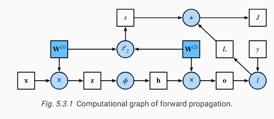
Plotting computational graphs helps us visualize the dependencies of operators and variables within the calculation. Fig. 5.3.1 contains the graph associated with the simple network described above, where squares denote variables and circles denote operators. The lower-left corner signifies the input and the upper-right corner is the output. Notice that the directions of the arrows (which illustrate data flow) are primarily rightward and upward.
계산 그래프를 플로팅하면 계산 내에서 연산자와 변수의 종속성을 시각화하는 데 도움이 됩니다. 그림 5.3.1은 위에서 설명한 간단한 네트워크와 관련된 그래프를 포함하고 있습니다. 여기서 사각형은 변수를 나타내고 원은 연산자를 나타냅니다. 왼쪽 하단 모서리는 입력을 나타내고 오른쪽 상단 모서리는 출력을 나타냅니다. 데이터 흐름을 나타내는 화살표의 방향은 주로 오른쪽과 위쪽입니다.
5.3.3. Backpropagation
Backpropagation refers to the method of calculating the gradient of neural network parameters. In short, the method traverses the network in reverse order, from the output to the input layer, according to the chain rule from calculus. The algorithm stores any intermediate variables (partial derivatives) required while calculating the gradient with respect to some parameters. Assume that we have functions Y=f(X) and Z=g(Y), in which the input and the output X,Y,Z are tensors of arbitrary shapes. By using the chain rule, we can compute the derivative of Z with respect to X via
역전파는 신경망 매개변수의 기울기를 계산하는 방법을 말합니다. 요컨대, 이 방법은 미적분학의 체인 규칙에 따라 출력에서 입력 계층까지 역순으로 네트워크를 통과합니다. 이 알고리즘은 일부 매개변수에 대한 기울기를 계산하는 동안 필요한 모든 중간 변수(부분 도함수)를 저장합니다. 입력 및 출력 X,Y,Z가 임의의 모양의 텐서인 함수 Y=f(X) 및 Z=g(Y)가 있다고 가정합니다. 체인 규칙을 사용하여 다음을 통해 X에 대한 Z의 도함수를 계산할 수 있습니다.
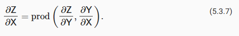
Here we use the prod operator to multiply its arguments after the necessary operations, such as transposition and swapping input positions, have been carried out. For vectors, this is straightforward: it is simply matrix-matrix multiplication. For higher dimensional tensors, we use the appropriate counterpart. The operator prod hides all the notation overhead.
여기에서 prod 연산자를 사용하여 전치 및 입력 위치 교환과 같은 필요한 작업이 수행된 후 인수를 곱합니다. 벡터의 경우 이것은 간단합니다. 단순히 행렬-행렬 곱셈입니다. 더 높은 차원의 텐서의 경우 적절한 상대를 사용합니다. 연산자 prod는 모든 표기 오버헤드를 숨깁니다.
Recall that the parameters of the simple network with one hidden layer, whose computational graph is in Fig. 5.3.1, are W(1) and W(2). The objective of backpropagation is to calculate the gradients aJ/aW(1) and aJ/aW(2). To accomplish this, we apply the chain rule and calculate, in turn, the gradient of each intermediate variable and parameter. The order of calculations are reversed relative to those performed in forward propagation, since we need to start with the outcome of the computational graph and work our way towards the parameters. The first step is to calculate the gradients of the objective function J=L+s with respect to the loss term L and the regularization term s.
계산 그래프가 그림 5.3.1에 있는 하나의 숨겨진 레이어가 있는 단순 네트워크의 매개 변수는 W(1) 및 W(2)입니다. 역전파의 목적은 그래디언트 aJ/aW(1) 및 aJ/aW(2)를 계산하는 것입니다. 이를 달성하기 위해 체인 규칙을 적용하고 각 중간 변수 및 매개변수의 기울기를 차례로 계산합니다. 계산 순서는 계산 그래프의 결과에서 시작하여 매개변수를 향해 작업해야 하기 때문에 정방향 전파에서 수행된 순서와 반대입니다. 첫 번째 단계는 손실 항 L과 정규화 항 s에 대한 목적 함수 J=L+s의 기울기를 계산하는 것입니다.

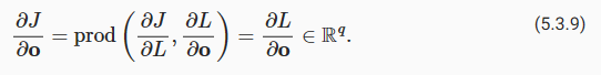
Next, we compute the gradient of the objective function with respect to variable of the output layer o according to the chain rule:
다음으로 체인 규칙에 따라 출력 레이어 o의 변수에 대한 목적 함수의 그래디언트를 계산합니다.
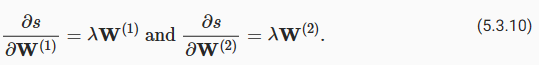
Next, we calculate the gradients of the regularization term with respect to both parameters:
다음으로 두 매개변수에 대한 정규화 항의 그래디언트를 계산합니다.
Now we are able to calculate the gradient aJ/aW(2)∈Rq×ℎ of the model parameters closest to the output layer. Using the chain rule yields:
이제 출력 레이어에 가장 가까운 모델 매개변수의 그래디언트 aJ/aW(2)∈Rq×ℎ를 계산할 수 있습니다. 체인 규칙을 사용하면 다음이 생성됩니다.

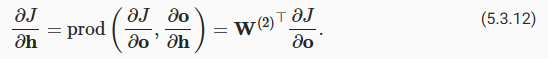
To obtain the gradient with respect to W(1) we need to continue backpropagation along the output layer to the hidden layer. The gradient with respect to the hidden layer output aJ/aℎ∈Rℎ is given by
W(1)에 대한 그래디언트를 얻으려면 출력 레이어를 따라 숨겨진 레이어까지 역전파를 계속해야 합니다. 은닉층 출력 aJ/aℎ∈Rℎ에 대한 그래디언트는 다음과 같습니다.
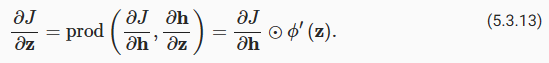
Since the activation function φ applies elementwise, calculating the gradient aJ/az∈Rℎ of the intermediate variable z requires that we use the elementwise multiplication operator, which we denote by ⊙:
활성화 함수 φ가 요소별로 적용되기 때문에 중간 변수 z의 기울기 aJ/az∈Rℎ를 계산하려면 ⊙로 표시되는 요소별 곱셈 연산자를 사용해야 합니다.
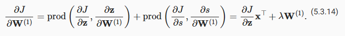
Finally, we can obtain the gradient aJ/aW(1)∈Rℎ×d of the model parameters closest to the input layer. According to the chain rule, we get
마지막으로 입력 레이어에 가장 가까운 모델 매개변수의 기울기 aJ/aW(1)∈Rℎ×d를 얻을 수 있습니다. 연쇄법칙에 따르면 아래와 같습니다.
Backpropagation이란?
Backpropagation is an algorithm used in neural networks to update the weights and biases by computing the gradients of the loss function. It is also known as backward propagation. Backpropagation involves propagating the error backwards through the network to calculate the gradients of the weights and biases in each layer.
Backpropagation은 신경망의 가중치와 편향을 업데이트하기 위해 손실 함수의 기울기를 계산하는 알고리즘입니다. Backpropagation은 역전파라고도 불리며, 오차를 역으로 전파하여 각 계층의 가중치와 편향에 대한 기울기를 계산하는 과정을 의미합니다.
The process of backpropagation starts by computing the loss between the network's output and the desired output. This loss is then used to propagate the error backwards through the network, layer by layer. This allows us to compute the gradients of the loss function with respect to the weights and biases. These gradients are then used to update the weights and biases using an optimization algorithm such as gradient descent.
Backpropagation은 신경망의 출력과 실제 값 사이의 손실을 계산한 후, 이 손실을 사용하여 역방향으로 오차를 전파합니다. 이를 통해 각 계층의 가중치와 편향에 대한 손실 함수의 기울기를 계산할 수 있습니다. 이 기울기는 경사 하강법과 같은 최적화 알고리즘을 사용하여 가중치와 편향을 업데이트하는 데 활용됩니다.
Backpropagation relies on the chain rule of calculus to compute the gradients efficiently. Starting from the output layer, the gradients are calculated with respect to the inputs of each layer and then propagated backwards to the previous layers. This process is repeated until the gradients of the loss function with respect to all the weights and biases have been computed.
Backpropagation은 연쇄 법칙을 기반으로 동작합니다. 출력 계층부터 시작하여 각 계층의 입력에 대한 기울기를 계산하고, 이를 이전 계층으로 전파합니다. 이러한 과정을 반복하여 입력 계층까지 진행하면 모든 가중치와 편향에 대한 기울기를 얻을 수 있습니다.
Backpropagation is used during the training phase of a neural network. By computing the gradients of the loss function, it allows the network to adjust its weights and biases to improve its predictions and generate optimal outputs for the given input data.
Backpropagation은 신경망의 학습 단계에서 사용되며, 손실 함수의 기울기를 계산하여 가중치와 편향을 업데이트합니다. 이를 통해 신경망은 예측을 개선하고 입력 데이터에 대한 최적의 출력을 생성할 수 있습니다.
In summary, backpropagation is an algorithm used in neural networks to update the weights and biases by computing the gradients of the loss function. It involves propagating the error backwards through the network, layer by layer, to compute the gradients. This process enables the network to learn and improve its predictions during training.
요약하면, Backpropagation은 신경망의 가중치와 편향을 업데이트하기 위해 손실 함수의 기울기를 계산하는 알고리즘으로, 역전파와 기울기 전파라고도 불립니다. 이 알고리즘은 신경망의 학습 과정에서 사용되며, 신경망의 출력과 실제 값 사이의 오차를 역으로 전파하여 가중치와 편향을 조정합니다.
5.3.4. Training Neural Networks
When training neural networks, forward and backward propagation depend on each other. In particular, for forward propagation, we traverse the computational graph in the direction of dependencies and compute all the variables on its path. These are then used for backpropagation where the compute order on the graph is reversed.
신경망을 훈련할 때 순방향 전파와 역방향 전파는 서로 의존합니다. 특히 정방향 전파의 경우 종속성 방향으로 계산 그래프를 순회하고 해당 경로의 모든 변수를 계산합니다. 그런 다음 그래프의 계산 순서가 반전되는 역전파에 사용됩니다.
Take the aforementioned simple network as an example to illustrate. On the one hand, computing the regularization term (5.3.5) during forward propagation depends on the current values of model parameters W(1) and W(2). They are given by the optimization algorithm according to backpropagation in the latest iteration. On the other hand, the gradient calculation for the parameter (5.3.11) during backpropagation depends on the current value of the hidden layer output ℎ, which is given by forward propagation.
설명을 위해 앞서 언급한 간단한 네트워크를 예로 들어 보겠습니다. 한편으로 정방향 전파 동안 정규화 항(5.3.5)을 계산하는 것은 모델 매개변수 W(1) 및 W(2)의 현재 값에 따라 달라집니다. 최신 반복에서 역전파에 따라 최적화 알고리즘에 의해 제공됩니다. 한편, 역전파 동안 매개변수(5.3.11)에 대한 그래디언트 계산은 순방향 전파에 의해 주어진 숨겨진 계층 출력 ℎ의 현재 값에 따라 달라집니다.
Therefore when training neural networks, after model parameters are initialized, we alternate forward propagation with backpropagation, updating model parameters using gradients given by backpropagation. Note that backpropagation reuses the stored intermediate values from forward propagation to avoid duplicate calculations. One of the consequences is that we need to retain the intermediate values until backpropagation is complete. This is also one of the reasons why training requires significantly more memory than plain prediction. Besides, the size of such intermediate values is roughly proportional to the number of network layers and the batch size. Thus, training deeper networks using larger batch sizes more easily leads to out of memory errors.
따라서 신경망을 훈련할 때 모델 매개변수가 초기화된 후 순전파와 역전파를 번갈아 가며 역전파에 의해 제공된 그래디언트를 사용하여 모델 매개변수를 업데이트합니다. 역전파는 중복 계산을 피하기 위해 정방향 전파에서 저장된 중간 값을 재사용합니다. 결과 중 하나는 역전파가 완료될 때까지 중간 값을 유지해야 한다는 것입니다. 이것은 훈련이 일반 예측보다 훨씬 더 많은 메모리를 필요로 하는 이유 중 하나이기도 합니다. 게다가 이러한 중간 값의 크기는 대략적으로 네트워크 계층의 수와 배치 크기에 비례합니다. 따라서 더 큰 배치 크기를 사용하여 더 깊은 네트워크를 훈련하면 메모리 부족 오류가 더 쉽게 발생합니다.
5.3.5. Summary
Forward propagation sequentially calculates and stores intermediate variables within the computational graph defined by the neural network. It proceeds from the input to the output layer. Backpropagation sequentially calculates and stores the gradients of intermediate variables and parameters within the neural network in the reversed order. When training deep learning models, forward propagation and back propagation are interdependent, and training requires significantly more memory than prediction.
정방향 전파는 신경망에 의해 정의된 계산 그래프 내에서 중간 변수를 순차적으로 계산하고 저장합니다. 입력 레이어에서 출력 레이어로 진행됩니다. 역전파는 신경망 내의 중간 변수와 매개변수의 기울기를 역순으로 순차적으로 계산하고 저장합니다. 딥 러닝 모델을 훈련할 때 전방 전파와 역전파는 상호 의존적이며 훈련에는 예측보다 훨씬 더 많은 메모리가 필요합니다.
5.3.6. Exercises
- Assume that the inputs X to some scalar function f are n×m matrices. What is the dimensionality of the gradient of f with respect to X?
- Add a bias to the hidden layer of the model described in this section (you do not need to include bias in the regularization term).
- Draw the corresponding computational graph.
- Derive the forward and backward propagation equations.
- Compute the memory footprint for training and prediction in the model described in this section.
- Assume that you want to compute second derivatives. What happens to the computational graph? How long do you expect the calculation to take?
- Assume that the computational graph is too large for your GPU.
- Can you partition it over more than one GPU?
- What are the advantages and disadvantages over training on a smaller minibatch?
'Dive into Deep Learning > D2L Multilayer Perceptrons Builder Guide' 카테고리의 다른 글
| D2L - 5.7. Predicting House Prices on Kaggle (0) | 2023.07.03 |
|---|---|
| D2L - 5.6. Dropout (0) | 2023.07.03 |
| D2L - 5.5. Generalization in Deep Learning (0) | 2023.07.03 |
| D2L - 5.4. Numerical Stability and Initialization (0) | 2023.07.02 |
| D2L - 5.2. Implementation of Multilayer Perceptrons (0) | 2023.07.01 |
| D2L - 5.1. Multilayer Perceptrons (0) | 2023.07.01 |
| D2L - 5. Multilayer Perceptrons (1) | 2023.06.30 |