개발자로서 현장에서 일하면서 새로 접하는 기술들이나 알게된 정보 등을 정리하기 위한 블로그입니다. 운 좋게 미국에서 큰 회사들의 프로젝트에서 컬설턴트로 일하고 있어서 새로운 기술들을 접할 기회가 많이 있습니다. 미국의 IT 프로젝트에서 사용되는 툴들에 대해 많은 분들과 정보를 공유하고 싶습니다.
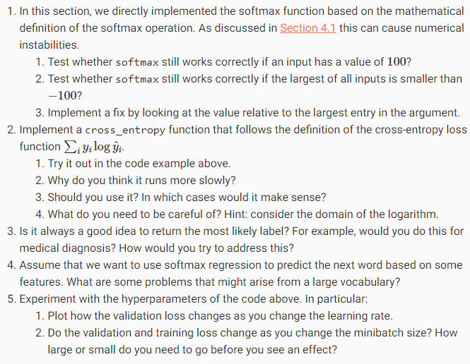
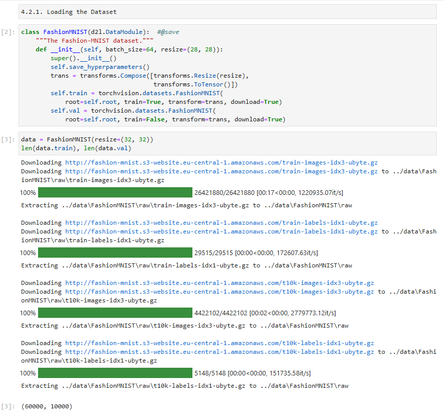
Now that we have characterized the problem of overfitting, we can introduce our firstregularizationtechnique. Recall that we can always mitigate overfitting by collecting more training data. However, that can be costly, time consuming, or entirely out of our control, making it impossible in the short run. For now, we can assume that we already have as much high-quality data as our resources permit and focus the tools at our disposal when the dataset is taken as a given.
이제 과적합 문제를 특성화했으므로 첫 번째 정규화 기술을 소개할 수 있습니다. 더 많은 훈련 데이터를 수집하면 항상 과적합을 완화할 수 있다는 점을 기억하세요. 그러나 이는 비용이 많이 들고, 시간이 많이 걸리거나 완전히 통제할 수 없어 단기적으로 불가능할 수 있습니다. 지금은 리소스가 허용하는 만큼의 고품질 데이터를 이미 보유하고 있다고 가정하고 데이터 세트를 주어진 것으로 간주할 때 사용할 수 있는 도구에 집중할 수 있습니다.
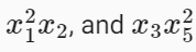
Recall that in our polynomial regression example (Section 3.6.2.1) we could limit our model’s capacity by tweaking the degree of the fitted polynomial. Indeed, limiting the number of features is a popular technique for mitigating overfitting. However, simply tossing aside features can be too blunt an instrument. Sticking with the polynomial regression example, consider what might happen with high-dimensional input. The natural extensions of polynomials to multivariate data are calledmonomials, which are simply products of powers of variables. The degree of a monomial is the sum of the powers. For example,x1**2x2, andx3x5**2 (
)are both monomials of degree 3.
다항식 회귀 예제(섹션 3.6.2.1)에서 피팅된 다항식의 차수를 조정하여 모델의 용량을 제한할 수 있다는 점을 기억하세요. 실제로 특성 수를 제한하는 것은 과적합을 완화하는 데 널리 사용되는 기술입니다. 그러나 단순히 기능을 제쳐두는 것은 너무 무뚝뚝한 도구가 될 수 있습니다. 다항식 회귀 예제를 계속 사용하면서 고차원 입력에서 어떤 일이 발생할 수 있는지 생각해 보세요. 다변량 데이터에 대한 다항식의 자연스러운 확장을 단항식이라고 하며 이는 단순히 변수 거듭제곱의 곱입니다. 단항식의 차수는 거듭제곱의 합입니다. 예를 들어 x1**2x2와 x3x5**2 ()는 모두 3차 단항식입니다.
Note that the number of terms with degreedblows up rapidly asdgrows larger. Givenkvariables, the number of monomials of degreedis(k−1+d k−1) (
). Even small changes in degree, say from2to3, dramatically increase the complexity of our model. Thus we often need a more fine-grained tool for adjusting function complexity.
d가 커짐에 따라 차수 d를 갖는 항의 수가 급격히 증가한다는 점에 유의하십시오. k개의 변수가 주어지면 d차 단항식의 수는 (k−1+d k−1)입니다. 2에서 3까지의 작은 변화조차도 모델의 복잡성을 극적으로 증가시킵니다. 따라서 함수 복잡성을 조정하기 위해 보다 세분화된 도구가 필요한 경우가 많습니다.
%matplotlib inline
import torch
from torch import nn
from d2l import torch as d2l
3.7.1.Norms and Weight Decay
Rather than directly manipulating the number of parameters,weight decay, operates by restricting the values that the parameters can take. More commonly calledℓ2regularization outside of deep learning circles when optimized by minibatch stochastic gradient descent, weight decay might be the most widely used technique for regularizing parametric machine learning models. The technique is motivated by the basic intuition that among all functionsf, the functionf=0(assigning the value0to all inputs) is in some sense thesimplest, and that we can measure the complexity of a function by the distance of its parameters from zero. But how precisely should we measure the distance between a function and zero? There is no single right answer. In fact, entire branches of mathematics, including parts of functional analysis and the theory of Banach spaces, are devoted to addressing such issues.
매개변수 수를 직접 조작하는 대신 가중치 감소는 매개변수가 취할 수 있는 값을 제한하여 작동합니다. 미니배치 확률적 경사 하강법으로 최적화할 때 딥 러닝 분야 외부에서 더 일반적으로 ℓ2 정규화라고 불리는 가중치 감소는 파라메트릭 기계 학습 모델을 정규화하는 데 가장 널리 사용되는 기술일 수 있습니다. 이 기술은 모든 함수 f 중에서 함수 f=0(모든 입력에 값 0을 할당하는)이 어떤 의미에서는 가장 단순하며 함수의 복잡성을 함수의 거리로 측정할 수 있다는 기본적인 직관에 의해 동기가 부여되었습니다. 매개변수는 0부터 시작됩니다. 하지만 함수와 0 사이의 거리를 얼마나 정확하게 측정해야 할까요? 정답은 하나도 없습니다. 실제로 기능 분석의 일부와 바나흐 공간 이론을 포함한 수학의 전체 분야가 이러한 문제를 해결하는 데 전념하고 있습니다.
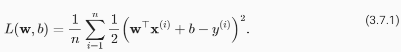
One simple interpretation might be to measure the complexity of a linear functionf(x)=w⊤xby some norm of its weight vector, e.g.,‖w‖**2. Recall that we introduced theℓ2norm andℓ1norm, which are special cases of the more generalℓpnorm, inSection 2.3.11. The most common method for ensuring a small weight vector is to add its norm as a penalty term to the problem of minimizing the loss. Thus we replace our original objective,minimizing the prediction loss on the training labels, with new objective,minimizing the sum of the prediction loss and the penalty term. Now, if our weight vector grows too large, our learning algorithm might focus on minimizing the weight norm‖w‖**2rather than minimizing the training error. That is exactly what we want. To illustrate things in code, we revive our previous example fromSection 3.1for linear regression. There, our loss was given by
한 가지 간단한 해석은 선형 함수 f(x)=w⊤x의 복잡성을 해당 가중치 벡터의 일부 표준(예: "w"**2)으로 측정하는 것입니다. 섹션 2.3.11에서 보다 일반적인 ℓp 노름의 특수한 경우인 ℓ2 노름과 ℓ1 노름을 소개했음을 기억하세요. 작은 가중치 벡터를 보장하는 가장 일반적인 방법은 손실을 최소화하는 문제에 페널티 항으로 해당 노름을 추가하는 것입니다. 따라서 우리는 훈련 라벨의 예측 손실을 최소화하는 원래 목표를 예측 손실과 페널티 항의 합을 최소화하는 새로운 목표로 대체합니다. 이제 가중치 벡터가 너무 커지면 학습 알고리즘은 훈련 오류를 최소화하는 대신 가중치 표준 "w"**2를 최소화하는 데 중점을 둘 수 있습니다. 그것이 바로 우리가 원하는 것입니다. 코드로 내용을 설명하기 위해 선형 회귀에 대한 섹션 3.1의 이전 예제를 되살립니다. 거기에서 우리의 손실은 다음과 같습니다.
Recall thatx**(i)are the features,y**(i)is the label for any data examplei, and(w,b)are the weight and bias parameters, respectively. To penalize the size of the weight vector, we must somehow add‖w‖**2to the loss function, but how should the model trade off the standard loss for this new additive penalty? In practice, we characterize this trade-off via theregularization constantλ, a nonnegative hyperparameter that we fit using validation data:
x**(i)는 특징이고, y**(i)는 데이터 예제 i에 대한 레이블이며, (w,b)는 각각 가중치 및 편향 매개변수라는 점을 기억하세요. 가중치 벡터의 크기에 페널티를 적용하려면 어떻게든 손실 함수에 "w"**2를 추가해야 합니다. 하지만 모델은 이 새로운 추가 페널티에 대한 표준 손실을 어떻게 교환해야 할까요? 실제로 우리는 검증 데이터를 사용하여 피팅한 음이 아닌 하이퍼파라미터인 정규화 상수 λ를 통해 이러한 절충안을 특성화합니다.
For λ =0, we recover our original loss function. For λ >0, we restrict the size of‖W‖. We divide by2by convention: when we take the derivative of a quadratic function, the2and1/2cancel out, ensuring that the expression for the update looks nice and simple. The astute reader might wonder why we work with the squared norm and not the standard norm (i.e., the Euclidean distance). We do this for computational convenience. By squaring theℓ2norm, we remove the square root, leaving the sum of squares of each component of the weight vector. This makes the derivative of the penalty easy to compute: the sum of derivatives equals the derivative of the sum.
λ =0인 경우 원래의 손실 함수를 복구합니다. λ >0인 경우 "W" 크기를 제한합니다. 관례에 따라 2로 나눕니다. 이차 함수의 미분을 취하면 2와 1/2이 상쇄되어 업데이트에 대한 식이 멋지고 단순해 보입니다. 기민한 독자라면 왜 우리가 표준 표준(예: 유클리드 거리)이 아닌 제곱 표준을 사용하여 작업하는지 궁금할 것입니다. 우리는 계산상의 편의를 위해 이렇게 합니다. ℓ2 노름을 제곱함으로써 제곱근을 제거하고 가중치 벡터의 각 구성요소의 제곱합을 남깁니다. 이는 페널티의 미분을 계산하기 쉽게 만듭니다. 미분의 합은 합계의 미분과 같습니다.
Moreover, you might ask why we work with theℓ2norm in the first place and not, say, theℓ1norm. In fact, other choices are valid and popular throughout statistics. Whileℓ2-regularized linear models constitute the classicridge regressionalgorithm,ℓ1-regularized linear regression is a similarly fundamental method in statistics, popularly known aslasso regression. One reason to work with theℓ2norm is that it places an outsize penalty on large components of the weight vector. This biases our learning algorithm towards models that distribute weight evenly across a larger number of features. In practice, this might make them more robust to measurement error in a single variable. By contrast,ℓ1penalties lead to models that concentrate weights on a small set of features by clearing the other weights to zero. This gives us an effective method forfeature selection, which may be desirable for other reasons. For example, if our model only relies on a few features, then we may not need to collect, store, or transmit data for the other (dropped) features.
게다가 왜 우리가 ℓ1 표준이 아닌 ℓ2 표준으로 작업하는지 궁금할 수도 있습니다. 실제로 통계 전반에 걸쳐 다른 선택이 유효하고 널리 사용됩니다. ℓ2 정규화 선형 모델이 고전적인 능선 회귀 알고리즘을 구성하는 반면, ℓ1 정규화 선형 회귀는 lasso 회귀로 널리 알려진 통계의 유사한 기본 방법입니다. ℓ2 표준을 사용하는 한 가지 이유는 가중치 벡터의 큰 구성요소에 특대 페널티를 적용한다는 것입니다. 이는 우리의 학습 알고리즘을 더 많은 수의 특성에 균등하게 가중치를 분배하는 모델로 편향시킵니다. 실제로 이는 단일 변수의 측정 오류에 더욱 강력해질 수 있습니다. 대조적으로, ℓ1 페널티는 다른 가중치를 0으로 지워서 작은 특성 집합에 가중치를 집중시키는 모델로 이어집니다. 이는 다른 이유로 바람직할 수 있는 특징 선택을 위한 효과적인 방법을 제공합니다. 예를 들어 모델이 몇 가지 기능에만 의존하는 경우 다른(삭제된) 기능에 대한 데이터를 수집, 저장 또는 전송할 필요가 없을 수 있습니다.
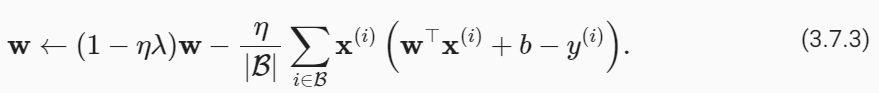
Using the same notation in(3.1.11), minibatch stochastic gradient descent updates forℓ2-regularized regression as follows:
(3.1.11)의 동일한 표기법을 사용하여 ℓ2 정규 회귀에 대한 미니배치 확률적 경사하강법 업데이트는 다음과 같습니다.
As before, we updatewbased on the amount by which our estimate differs from the observation. However, we also shrink the size of wtowards zero. That is why the method is sometimes called “weight decay”: given the penalty term alone, our optimization algorithmdecaysthe weight at each step of training. In contrast to feature selection, weight decay offers us a mechanism for continuously adjusting the complexity of a function. Smaller values of λ correspond to less constrainedw, whereas larger values of λ constrainwmore considerably. Whether we include a corresponding bias penaltyb**2can vary across implementations, and may vary across layers of a neural network. Often, we do not regularize the bias term. Besides, althoughℓ2regularization may not be equivalent to weight decay for other optimization algorithms, the idea of regularization through shrinking the size of weights still holds true.
이전과 마찬가지로 추정값이 관측값과 다른 정도에 따라 w를 업데이트합니다. 그러나 w의 크기도 0으로 축소합니다. 이것이 바로 이 방법을 "가중치 감소"라고 부르는 이유입니다. 페널티 항만 주어지면 우리의 최적화 알고리즘은 훈련의 각 단계에서 가중치를 감소시킵니다. 기능 선택과 달리 가중치 감소는 기능의 복잡성을 지속적으로 조정하는 메커니즘을 제공합니다. λ의 값이 작을수록 w가 덜 제한되는 반면, λ의 값이 클수록 w가 더 크게 제한됩니다. 해당 바이어스 페널티 b**2를 포함하는지 여부는 구현에 따라 다를 수 있으며 신경망의 계층에 따라 다를 수 있습니다. 종종 우리는 편향 항을 정규화하지 않습니다. 게다가 ℓ2 정규화는 다른 최적화 알고리즘의 가중치 감소와 동일하지 않을 수 있지만 가중치 크기 축소를 통한 정규화 아이디어는 여전히 유효합니다.
3.7.2.High-Dimensional Linear Regression
We can illustrate the benefits of weight decay through a simple synthetic example.
간단한 합성 예를 통해 체중 감소의 이점을 설명할 수 있습니다.
First, we generate some data as before:
먼저 이전과 같이 일부 데이터를 생성합니다.
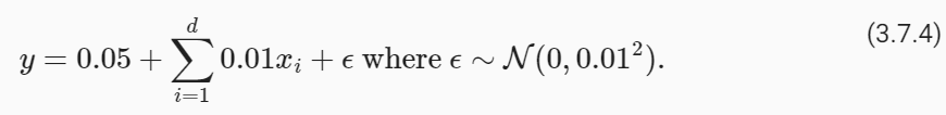
In this synthetic dataset, our label is given by an underlying linear function of our inputs, corrupted by Gaussian noise with zero mean and standard deviation 0.01. For illustrative purposes, we can make the effects of overfitting pronounced, by increasing the dimensionality of our problem to d=200and working with a small training set with only 20 examples.
이 합성 데이터 세트에서 레이블은 평균이 0이고 표준 편차가 0.01인 가우스 노이즈로 인해 손상된 입력의 기본 선형 함수로 제공됩니다. 설명을 위해 문제의 차원을 d=200으로 늘리고 20개의 예제만 있는 작은 훈련 세트로 작업하여 과적합의 효과를 뚜렷하게 만들 수 있습니다.
class Data(d2l.DataModule):
    def __init__(self, num_train, num_val, num_inputs, batch_size):
        self.save_hyperparameters()
        n = num_train + num_val
        self.X = torch.randn(n, num_inputs)
        noise = torch.randn(n, 1) * 0.01
        w, b = torch.ones((num_inputs, 1)) * 0.01, 0.05
        self.y = torch.matmul(self.X, w) + b + noise

    def get_dataloader(self, train):
        i = slice(0, self.num_train) if train else slice(self.num_train, None)
        return self.get_tensorloader([self.X, self.y], train, i)
3.7.3.Implementation from Scratc
Now, let’s try implementing weight decay from scratch. Since minibatch stochastic gradient descent is our optimizer, we just need to add the squaredℓ2penalty to the original loss function.
이제 처음부터 가중치 감소를 구현해 보겠습니다. 미니배치 확률적 경사하강법이 우리의 최적화 프로그램이므로 원래 손실 함수에 제곱된 ℓ2 페널티를 추가하기만 하면 됩니다.
3.7.3.1.Definingℓ2Norm Penalty
Perhaps the most convenient way of implementing this penalty is to square all terms in place and sum them.
아마도 이 페널티를 구현하는 가장 편리한 방법은 모든 항을 제곱하고 합하는 것입니다.
def l2_penalty(w):
    return (w ** 2).sum() / 2
3.7.3.2.Defining the Model
In the final model, the linear regression and the squared loss have not changed sinceSection 3.4, so we will just define a subclass ofd2l.LinearRegressionScratch. The only change here is that our loss now includes the penalty term.
최종 모델에서는 선형 회귀와 제곱 손실이 섹션 3.4 이후로 변경되지 않았으므로 d2l.LinearRegressionScratch의 하위 클래스만 정의하겠습니다. 여기서 유일한 변경 사항은 이제 손실에 페널티 기간이 포함된다는 것입니다.
The following code fits our model on the training set with 20 examples and evaluates it on the validation set with 100 examples.
다음 코드는 20개의 예제가 있는 훈련 세트에 모델을 맞추고 100개의 예제가 있는 검증 세트에서 모델을 평가합니다.
data = Data(num_train=20, num_val=100, num_inputs=200, batch_size=5)
trainer = d2l.Trainer(max_epochs=10)

def train_scratch(lambd):
    model = WeightDecayScratch(num_inputs=200, lambd=lambd, lr=0.01)
    model.board.yscale='log'
    trainer.fit(model, data)
    print('L2 norm of w:', float(l2_penalty(model.w)))
3.7.3.3.Training without Regularization
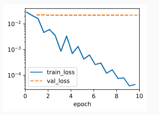
We now run this code withlambd=0, disabling weight decay. Note that we overfit badly, decreasing the training error but not the validation error—a textbook case of overfitting.
이제 이 코드를 Lambd = 0으로 실행하여 가중치 감소를 비활성화합니다. 우리는 과적합을 심하게 하여 학습 오류를 줄였지만 검증 오류는 줄이지 않았습니다. 이는 과적합의 교과서적인 사례입니다.
train_scratch(0)
L2 norm of w: 0.009948714636266232
3.7.3.4.Using Weight Decay
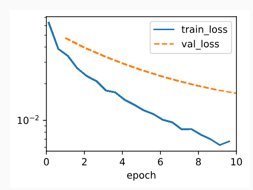
Below, we run with substantial weight decay. Note that the training error increases but the validation error decreases. This is precisely the effect we expect from regularization.
아래에서는 상당한 체중 감소를 보여줍니다. 학습 오류는 증가하지만 검증 오류는 감소합니다. 이것이 바로 우리가 정규화에서 기대하는 효과입니다.
train_scratch(3)
L2 norm of w: 0.0017270983662456274
3.7.4.Concise Implementation
Because weight decay is ubiquitous in neural network optimization, the deep learning framework makes it especially convenient, integrating weight decay into the optimization algorithm itself for easy use in combination with any loss function. Moreover, this integration serves a computational benefit, allowing implementation tricks to add weight decay to the algorithm, without any additional computational overhead. Since the weight decay portion of the update depends only on the current value of each parameter, the optimizer must touch each parameter once anyway.
가중치 감소는 신경망 최적화에서 어디에나 존재하기 때문에 딥 러닝 프레임워크는 모든 손실 함수와 결합하여 쉽게 사용할 수 있도록 최적화 알고리즘 자체에 가중치 감소를 통합하여 이를 특히 편리하게 만듭니다. 또한 이러한 통합은 추가 계산 오버헤드 없이 알고리즘에 가중치 감소를 추가하는 구현 트릭을 허용하므로 계산상의 이점을 제공합니다. 업데이트의 가중치 감소 부분은 각 매개변수의 현재 값에만 의존하므로 최적화 프로그램은 어쨌든 각 매개변수를 한 번 터치해야 합니다.
Below, we specify the weight decay hyperparameter directly throughweight_decaywhen instantiating our optimizer. By default, PyTorch decays both weights and biases simultaneously, but we can configure the optimizer to handle different parameters according to different policies. Here, we only setweight_decayfor the weights (thenet.weightparameters), hence the bias (thenet.biasparameter) will not decay.
아래에서는 최적화 프로그램을 인스턴스화할 때 Weight_decay를 통해 직접 가중치 감소 하이퍼파라미터를 지정합니다. 기본적으로 PyTorch는 가중치와 편향을 동시에 감소시키지만, 다양한 정책에 따라 다양한 매개변수를 처리하도록 최적화 프로그램을 구성할 수 있습니다. 여기서는 가중치(net.weight 매개변수)에 대해서만 Weight_decay를 설정하므로 편향(net.bias 매개변수)은 감소하지 않습니다.
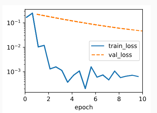
The plot looks similar to that when we implemented weight decay from scratch. However, this version runs faster and is easier to implement, benefits that will become more pronounced as you address larger problems and this work becomes more routine.
플롯은 처음부터 가중치 감소를 구현했을 때와 유사해 보입니다. 그러나 이 버전은 더 빠르게 실행되고 구현하기가 더 쉬우므로 더 큰 문제를 해결하고 이 작업이 더 일상화될수록 이점이 더욱 뚜렷해집니다.
model = WeightDecay(wd=3, lr=0.01)
model.board.yscale='log'
trainer.fit(model, data)

print('L2 norm of w:', float(l2_penalty(model.get_w_b()[0])))
L2 norm of w: 0.013779522851109505
So far, we have touched upon one notion of what constitutes a simple linear function. However, even for simple nonlinear functions, the situation can be much more complex. To see this, the concept ofreproducing kernel Hilbert space (RKHS)allows one to apply tools introduced for linear functions in a nonlinear context. Unfortunately, RKHS-based algorithms tend to scale poorly to large, high-dimensional data. In this book we will often adopt the common heuristic whereby weight decay is applied to all layers of a deep network.
지금까지 우리는 단순한 선형 함수를 구성하는 개념 중 하나를 다루었습니다. 그러나 단순한 비선형 함수의 경우에도 상황은 훨씬 더 복잡할 수 있습니다. 이를 확인하기 위해 RKHS(커널 힐베르트 공간 재현) 개념을 사용하면 비선형 맥락에서 선형 함수에 대해 도입된 도구를 적용할 수 있습니다. 불행하게도 RKHS 기반 알고리즘은 대규모 고차원 데이터에 제대로 확장되지 않는 경향이 있습니다. 이 책에서 우리는 딥 네트워크의 모든 계층에 가중치 감소를 적용하는 일반적인 경험적 방법을 자주 채택할 것입니다.
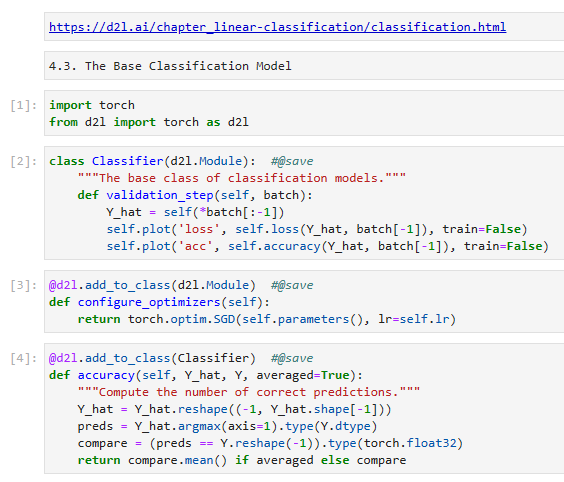
3.7.5.Summary
Regularization is a common method for dealing with overfitting. Classical regularization techniques add a penalty term to the loss function (when training) to reduce the complexity of the learned model. One particular choice for keeping the model simple is using anℓ2penalty. This leads to weight decay in the update steps of the minibatch stochastic gradient descent algorithm. In practice, the weight decay functionality is provided in optimizers from deep learning frameworks. Different sets of parameters can have different update behaviors within the same training loop.
정규화는 과적합을 처리하는 일반적인 방법입니다. 고전적인 정규화 기술은 학습된 모델의 복잡성을 줄이기 위해 (훈련 시) 손실 함수에 페널티 항을 추가합니다. 모델을 단순하게 유지하기 위한 한 가지 특별한 선택은 다음을 사용하는 것입니다. 패널티. 이로 인해 미니배치 확률적 경사하강법 알고리즘의 업데이트 단계에서 가중치 감소가 발생합니다. 실제로 가중치 감소 기능은 딥러닝 프레임워크의 최적화 프로그램에서 제공됩니다. 서로 다른 매개변수 세트는 동일한 훈련 루프 내에서 서로 다른 업데이트 동작을 가질 수 있습니다.
Consider two college students diligently preparing for their final exam. Commonly, this preparation will consist of practicing and testing their abilities by taking exams administered in previous years. Nonetheless, doing well on past exams is no guarantee that they will excel when it matters. For instance, imagine a student, Extraordinary Ellie, whose preparation consisted entirely of memorizing the answers to previous years’ exam questions. Even if Ellie were endowed with an extraordinary memory, and thus could perfectly recall the answer to anypreviously seenquestion, she might nevertheless freeze when faced with a new (previously unseen) question. By comparison, imagine another student, Inductive Irene, with comparably poor memorization skills, but a knack for picking up patterns. Note that if the exam truly consisted of recycled questions from a previous year, Ellie would handily outperform Irene. Even if Irene’s inferred patterns yielded 90% accurate predictions, they could never compete with Ellie’s 100% recall. However, even if the exam consisted entirely of fresh questions, Irene might maintain her 90% average.
최종 시험을 부지런히 준비하는 두 명의 대학생을 생각해 보십시오. 일반적으로 이 준비는 전년도에 시행된 시험을 통해 자신의 능력을 연습하고 테스트하는 것으로 구성됩니다. 그럼에도 불구하고 과거 시험에서 좋은 성적을 냈다고 해서 중요한 순간에 뛰어난 성적을 거둘 것이라는 보장은 없습니다. 예를 들어, 전년도 시험 문제에 대한 답을 암기하는 것만으로 준비를 했던 Extraordinary Ellie라는 학생을 상상해 보십시오. Ellie가 특별한 기억력을 부여받아 이전에 본 질문에 대한 답을 완벽하게 기억할 수 있다고 하더라도 새로운(이전에는 볼 수 없었던) 질문에 직면하면 그녀는 얼어붙을 수도 있습니다. 이에 비해 암기 능력은 비교적 낮지만 패턴을 파악하는 능력이 있는 또 다른 학생인 Induction Irene을 상상해 보십시오. 시험이 실제로 전년도의 질문을 재활용하여 구성되었다면 Ellie가 Irene보다 더 좋은 성적을 냈을 것입니다. 아이린이 추론한 패턴이 90% 정확한 예측을 내놨다고 해도 엘리의 100% 회상과 결코 경쟁할 수는 없습니다. 그러나 시험이 완전히 새로운 문제로 구성되더라도 아이린은 평균 90%를 유지할 수 있습니다.
As machine learning scientists, our goal is to discoverpatterns. But how can we be sure that we have truly discovered ageneralpattern and not simply memorized our data? Most of the time, our predictions are only useful if our model discovers such a pattern. We do not want to predict yesterday’s stock prices, but tomorrow’s. We do not need to recognize already diagnosed diseases for previously seen patients, but rather previously undiagnosed ailments in previously unseen patients. This problem—how to discover patterns thatgeneralize—is the fundamental problem of machine learning, and arguably of all of statistics. We might cast this problem as just one slice of a far grander question that engulfs all of science: when are we ever justified in making the leap from particular observations to more general statements?
기계 학습 과학자로서 우리의 목표는 패턴을 발견하는 것입니다. 하지만 단순히 데이터를 암기한 것이 아니라 실제로 일반적인 패턴을 발견했다는 것을 어떻게 확신할 수 있습니까? 대부분의 경우 예측은 모델이 그러한 패턴을 발견한 경우에만 유용합니다. 우리는 어제의 주가를 예측하고 싶지 않고 내일의 주가를 예측하고 싶습니다. 우리는 이전에 본 환자에 대해 이미 진단된 질병을 인식할 필요가 없으며, 이전에 보지 못한 환자의 이전에 진단되지 않은 질병을 인식할 필요가 있습니다. 일반화되는 패턴을 발견하는 방법이라는 문제는 기계 학습과 모든 통계의 근본적인 문제입니다. 우리는 이 문제를 모든 과학을 포괄하는 훨씬 더 큰 질문의 한 조각으로 간주할 수 있습니다. 특정 관찰에서 보다 일반적인 진술로 도약하는 것이 언제 정당화될 수 있습니까?
In real life, we must fit our models using a finite collection of data. The typical scales of that data vary wildly across domains. For many important medical problems, we can only access a few thousand data points. When studying rare diseases, we might be lucky to access hundreds. By contrast, the largest public datasets consisting of labeled photographs, e.g., ImageNet(Denget al., 2009), contain millions of images. And some unlabeled image collections such as the Flickr YFC100M dataset can be even larger, containing over 100 million images(Thomeeet al., 2016). However, even at this extreme scale, the number of available data points remains infinitesimally small compared to the space of all possible images at a megapixel resolution. Whenever we work with finite samples, we must keep in mind the risk that we might fit our training data, only to discover that we failed to discover a generalizable pattern.
실생활에서는 유한한 데이터 모음을 사용하여 모델을 맞춰야 합니다. 해당 데이터의 일반적인 규모는 도메인에 따라 크게 다릅니다. 많은 중요한 의료 문제의 경우 우리는 수천 개의 데이터 포인트에만 접근할 수 있습니다. 희귀 질병을 연구할 때 운이 좋게도 수백 가지 질병에 접근할 수 있습니다. 대조적으로, ImageNet(Deng et al., 2009)과 같이 레이블이 지정된 사진으로 구성된 가장 큰 공개 데이터 세트에는 수백만 개의 이미지가 포함되어 있습니다. 그리고 Flickr YFC100M 데이터 세트와 같은 일부 레이블이 없는 이미지 컬렉션은 1억 개가 넘는 이미지를 포함하여 훨씬 더 클 수 있습니다(Thomee et al., 2016). 그러나 이러한 극단적인 규모에서도 사용 가능한 데이터 포인트의 수는 메가픽셀 해상도에서 가능한 모든 이미지의 공간에 비해 무한히 작은 상태로 유지됩니다. 유한한 샘플로 작업할 때마다 훈련 데이터를 적합했지만 일반화 가능한 패턴을 발견하지 못했다는 사실을 발견하게 될 위험을 염두에 두어야 합니다.
The phenomenon of fitting closer to our training data than to the underlying distribution is calledoverfitting, and techniques for combatting overfitting are often calledregularizationmethods. While it is no substitute for a proper introduction to statistical learning theory (seeBoucheronet al.(2005), Vapnik (1998)), we will give you just enough intuition to get going. We will revisit generalization in many chapters throughout the book, exploring both what is known about the principles underlying generalization in various models, and also heuristic techniques that have been found (empirically) to yield improved generalization on tasks of practical interest.
기본 분포보다 훈련 데이터에 더 가깝게 피팅되는 현상을 과적합이라고 하며, 과적합을 방지하는 기술을 종종 정규화 방법이라고 합니다. 이것이 통계적 학습 이론에 대한 적절한 소개를 대체할 수는 없지만(Boucheron et al.(2005), Vapnik(1998) 참조), 시작하는 데 충분한 직관을 제공할 것입니다. 우리는 다양한 모델의 일반화 기본 원리에 대해 알려진 내용과 실제 관심 있는 작업에 대해 개선된 일반화를 산출하기 위해 (경험적으로) 발견된 경험적 기법을 탐구하면서 책 전체의 여러 장에서 일반화를 다시 살펴볼 것입니다.
3.6.1.Training Error and Generalization Error
In the standard supervised learning setting, we assume that the training data and the test data are drawnindependentlyfromidenticaldistributions. This is commonly called theIID assumption. While this assumption is strong, it is worth noting that, absent any such assumption, we would be dead in the water. Why should we believe that training data sampled from distributionP(X,Y)should tell us how to make predictions on test data generated by adifferent distributionQ(X,Y)? Making such leaps turns out to require strong assumptions about howPand Qare related. Later on we will discuss some assumptions that allow for shifts in distribution but first we need to understand the IID case, whereP(⋅)=Q(⋅).
표준 지도 학습 설정에서는 훈련 데이터와 테스트 데이터가 동일한 분포에서 독립적으로 추출된다고 가정합니다. 이를 일반적으로 IID 가정이라고 합니다. 이 가정은 강력하지만, 그러한 가정이 없다면 우리는 물 속에서 죽을 것이라는 점은 주목할 가치가 있습니다. 분포 P(X,Y)에서 샘플링된 훈련 데이터가 다른 분포 Q(X,Y)에 의해 생성된 테스트 데이터에 대해 예측하는 방법을 알려주어야 하는 이유는 무엇입니까? 그러한 도약을 위해서는 P와 Q가 어떻게 관련되어 있는지에 대한 강력한 가정이 필요하다는 것이 밝혀졌습니다. 나중에 우리는 분포의 변화를 허용하는 몇 가지 가정에 대해 논의할 것이지만 먼저 P(⋅)=Q(⋅)인 IID 사례를 이해해야 합니다.
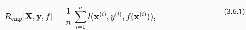
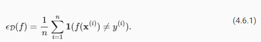
To begin with, we need to differentiate between thetraining errorRemp, which is astatisticcalculated on the training dataset, and thegeneralization errorR, which is anexpectationtaken with respect to the underlying distribution. You can think of the generalization error as what you would see if you applied your model to an infinite stream of additional data examples drawn from the same underlying data distribution. Formally the training error is expressed as asum(with the same notation asSection 3.1):
우선, 훈련 데이터세트에서 계산된 통계인 훈련 오류 Remp와 기본 분포에 대한 기대값인 일반화 오류 R을 구별해야 합니다. 일반화 오류는 동일한 기본 데이터 분포에서 추출된 추가 데이터 예제의 무한한 스트림에 모델을 적용한 경우 표시되는 오류로 생각할 수 있습니다. 공식적으로 훈련 오류는 합계로 표현됩니다(섹션 3.1과 동일한 표기법 사용).
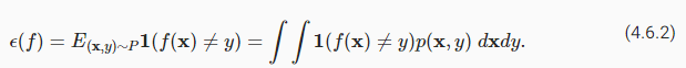
while the generalization error is expressed as an integral:
일반화 오류는 적분으로 표현됩니다.
Problematically, we can never calculate the generalization errorRexactly. Nobody ever tells us the precise form of the density functionp(x,y). Moreover, we cannot sample an infinite stream of data points. Thus, in practice, we mustestimatethe generalization error by applying our model to an independent test set constituted of a random selection of examplesX′and labelsy′that were withheld from our training set. This consists of applying the same formula that was used for calculating the empirical training error but to a test setX′,y′.
문제는 일반화 오류 R을 정확하게 계산할 수 없다는 점입니다. 밀도 함수 p(x,y)의 정확한 형태를 알려주는 사람은 아무도 없습니다. 게다가 무한한 데이터 포인트 스트림을 샘플링할 수도 없습니다. 따라서 실제로는 훈련 세트에서 보류된 X' 및 레이블 y'의 무작위 선택으로 구성된 독립적인 테스트 세트에 모델을 적용하여 일반화 오류를 추정해야 합니다. 이는 경험적 훈련 오류를 계산하는 데 사용된 것과 동일한 공식을 테스트 세트 X',y'에 적용하는 것으로 구성됩니다.
Crucially, when we evaluate our classifier on the test set, we are working with afixedclassifier (it does not depend on the sample of the test set), and thus estimating its error is simply the problem of mean estimation. However the same cannot be said for the training set. Note that the model we wind up with depends explicitly on the selection of the training set and thus the training error will in general be a biased estimate of the true error on the underlying population. The central question of generalization is then when should we expect our training error to be close to the population error (and thus the generalization error).
결정적으로 테스트 세트에서 분류기를 평가할 때 고정된 분류기를 사용하여 작업하므로(테스트 세트의 샘플에 의존하지 않음) 오류를 추정하는 것은 단순히 평균 추정의 문제입니다. 그러나 훈련 세트에 대해서도 마찬가지입니다. 우리가 마무리하는 모델은 훈련 세트의 선택에 명시적으로 의존하므로 훈련 오류는 일반적으로 기본 모집단의 실제 오류에 대한 편향된 추정치입니다. 일반화의 핵심 질문은 언제 훈련 오류가 모집단 오류(따라서 일반화 오류)에 가까워질 것으로 예상해야 하는가입니다.
3.6.1.1.Model Complexit
In classical theory, when we have simple models and abundant data, the training and generalization errors tend to be close. However, when we work with more complex models and/or fewer examples, we expect the training error to go down but the generalization gap to grow. This should not be surprising. Imagine a model class so expressive that for any dataset ofnexamples, we can find a set of parameters that can perfectly fit arbitrary labels, even if randomly assigned. In this case, even if we fit our training data perfectly, how can we conclude anything about the generalization error? For all we know, our generalization error might be no better than random guessing.
고전 이론에서는 단순한 모델과 풍부한 데이터가 있을 때 훈련 및 일반화 오류가 가까운 경향이 있습니다. 그러나 더 복잡한 모델 및/또는 더 적은 수의 예제를 사용하면 학습 오류는 줄어들지만 일반화 격차는 커질 것으로 예상됩니다. 이것은 놀라운 일이 아닙니다. n개의 예제로 구성된 데이터세트에 대해 무작위로 할당되더라도 임의의 레이블에 완벽하게 맞는 매개변수 집합을 찾을 수 있을 만큼 표현력이 뛰어난 모델 클래스를 상상해 보세요. 이 경우 훈련 데이터를 완벽하게 적합하더라도 일반화 오류에 대해 어떻게 결론을 내릴 수 있습니까? 우리가 아는 한, 일반화 오류는 무작위 추측보다 나을 것이 없을 수도 있습니다.
In general, absent any restriction on our model class, we cannot conclude, based on fitting the training data alone, that our model has discovered any generalizable pattern(Vapniket al., 1994). On the other hand, if our model class was not capable of fitting arbitrary labels, then it must have discovered a pattern. Learning-theoretic ideas about model complexity derived some inspiration from the ideas of Karl Popper, an influential philosopher of science, who formalized the criterion of falsifiability. According to Popper, a theory that can explain any and all observations is not a scientific theory at all! After all, what has it told us about the world if it has not ruled out any possibility? In short, what we want is a hypothesis thatcould notexplain any observations we might conceivably make and yet nevertheless happens to be compatible with those observations that wein factmake.
일반적으로 모델 클래스에 대한 제한이 없으면 훈련 데이터만 피팅하는 것만으로는 모델이 일반화 가능한 패턴을 발견했다고 결론을 내릴 수 없습니다(Vapnik et al., 1994). 반면, 모델 클래스가 임의의 레이블을 맞출 수 없다면 패턴을 발견했을 것입니다. 모델 복잡성에 대한 학습 이론적인 아이디어는 반증 가능성의 기준을 공식화한 영향력 있는 과학 철학자 칼 포퍼(Karl Popper)의 아이디어에서 영감을 얻었습니다. 포퍼에 따르면, 모든 관찰을 설명할 수 있는 이론은 전혀 과학 이론이 아닙니다! 결국, 어떤 가능성도 배제하지 않는다면 세상은 우리에게 무엇을 말해주는 것일까요? 간단히 말해서, 우리가 원하는 것은 우리가 할 수 있는 어떤 관찰도 설명할 수 없지만 그럼에도 불구하고 실제로 우리가 하는 관찰과 양립할 수 있는 가설입니다.
Now what precisely constitutes an appropriate notion of model complexity is a complex matter. Often, models with more parameters are able to fit a greater number of arbitrarily assigned labels. However, this is not necessarily true. For instance, kernel methods operate in spaces with infinite numbers of parameters, yet their complexity is controlled by other means(Schölkopf and Smola, 2002). One notion of complexity that often proves useful is the range of values that the parameters can take. Here, a model whose parameters are permitted to take arbitrary values would be more complex. We will revisit this idea in the next section, when we introduceweight decay, your first practical regularization technique. Notably, it can be difficult to compare complexity among members of substantially different model classes (say, decision trees vs. neural networks).
이제 모델 복잡성에 대한 적절한 개념을 정확히 구성하는 것은 복잡한 문제입니다. 매개변수가 더 많은 모델은 임의로 할당된 레이블을 더 많이 수용할 수 있는 경우가 많습니다. 그러나 이것이 반드시 사실은 아닙니다. 예를 들어, 커널 방법은 무한한 수의 매개변수가 있는 공간에서 작동하지만 그 복잡성은 다른 수단으로 제어됩니다(Schölkopf 및 Smola, 2002). 종종 유용하다고 입증되는 복잡성에 대한 한 가지 개념은 매개변수가 취할 수 있는 값의 범위입니다. 여기서 매개변수가 임의의 값을 취하도록 허용된 모델은 더 복잡합니다. 첫 번째 실용적인 정규화 기술인 가중치 감소를 소개하는 다음 섹션에서 이 아이디어를 다시 살펴보겠습니다. 특히, 실질적으로 다른 모델 클래스(예: 의사결정 트리와 신경망)의 구성원 간의 복잡성을 비교하는 것은 어려울 수 있습니다.
At this point, we must stress another important point that we will revisit when introducing deep neural networks. When a model is capable of fitting arbitrary labels, low training error does not necessarily imply low generalization error.However, it does not necessarily imply high generalization error either!All we can say with confidence is that low training error alone is not enough to certify low generalization error. Deep neural networks turn out to be just such models: while they generalize well in practice, they are too powerful to allow us to conclude much on the basis of training error alone. In these cases we must rely more heavily on our holdout data to certify generalization after the fact. Error on the holdout data, i.e., validation set, is called thevalidation error.
이 시점에서 우리는 심층 신경망을 도입할 때 다시 살펴볼 또 다른 중요한 점을 강조해야 합니다. 모델이 임의의 레이블을 맞출 수 있는 경우 훈련 오류가 낮다고 해서 반드시 일반화 오류가 낮다는 의미는 아닙니다. 그러나 이것이 반드시 높은 일반화 오류를 의미하는 것은 아닙니다! 우리가 자신있게 말할 수 있는 것은 낮은 훈련 오류만으로는 낮은 일반화 오류를 인증하는 데 충분하지 않다는 것입니다. 심층 신경망은 바로 그러한 모델임이 밝혀졌습니다. 실제로는 잘 일반화되지만 훈련 오류만으로 많은 결론을 내릴 수 없을 정도로 강력합니다. 이러한 경우 사실 이후 일반화를 인증하기 위해 홀드아웃 데이터에 더 많이 의존해야 합니다. 홀드아웃 데이터, 즉 검증 세트에 대한 오류를 검증 오류라고 합니다.
3.6.2.Underfitting or Overfitting?
When we compare the training and validation errors, we want to be mindful of two common situations. First, we want to watch out for cases when our training error and validation error are both substantial but there is a little gap between them. If the model is unable to reduce the training error, that could mean that our model is too simple (i.e., insufficiently expressive) to capture the pattern that we are trying to model. Moreover, since thegeneralization gap(Remp−R) between our training and generalization errors is small, we have reason to believe that we could get away with a more complex model. This phenomenon is known asunderfitting.
훈련 오류와 검증 오류를 비교할 때 두 가지 일반적인 상황에 유의하고 싶습니다. 먼저, 훈련 오류와 검증 오류가 모두 상당하지만 그 사이에 약간의 차이가 있는 경우를 주의하고 싶습니다. 모델이 훈련 오류를 줄일 수 없다면 이는 모델이 너무 단순하여(즉, 표현력이 부족하여) 모델링하려는 패턴을 포착할 수 없음을 의미할 수 있습니다. 더욱이 훈련 오류와 일반화 오류 사이의 일반화 격차(Remp-R)가 작기 때문에 더 복잡한 모델을 사용하여 벗어날 수 있다고 믿을 이유가 있습니다. 이 현상을 과소적합이라고 합니다.
On the other hand, as we discussed above, we want to watch out for the cases when our training error is significantly lower than our validation error, indicating severeoverfitting. Note that overfitting is not always a bad thing. In deep learning especially, the best predictive models often perform far better on training data than on holdout data. Ultimately, we usually care about driving the generalization error lower, and only care about the gap insofar as it becomes an obstacle to that end. Note that if the training error is zero, then the generalization gap is precisely equal to the generalization error and we can make progress only by reducing the gap.
반면, 위에서 논의한 것처럼 훈련 오류가 검증 오류보다 현저히 낮아 심각한 과적합을 나타내는 경우를 주의해야 합니다. 과적합이 항상 나쁜 것은 아닙니다. 특히 딥 러닝에서는 최고의 예측 모델이 홀드아웃 데이터보다 훈련 데이터에서 훨씬 더 나은 성능을 발휘하는 경우가 많습니다. 궁극적으로 우리는 일반적으로 일반화 오류를 낮추는 데 관심을 갖고, 그 목적에 장애물이 되는 한 격차에만 관심을 갖습니다. 훈련 오류가 0이면 일반화 격차는 일반화 오류와 정확하게 동일하며 격차를 줄여야만 진전을 이룰 수 있습니다.
3.6.2.1.Polynomial Curve Fitting
To illustrate some classical intuition about overfitting and model complexity, consider the following: given training data consisting of a single feature xand a corresponding real-valued labely, we try to find the polynomial of degree d for estimating the labely.
과적합 및 모델 복잡성에 대한 몇 가지 고전적 직관을 설명하기 위해 다음을 고려하십시오. 단일 특성 x와 해당 실제 값 레이블 y로 구성된 훈련 데이터가 주어지면 레이블 y를 추정하기 위해 d차 다항식을 찾으려고 합니다.
This is just a linear regression problem where our features are given by the powers ofx, the model’s weights are given bywi, and the bias is given byw0sincex**0=1for allx. Since this is just a linear regression problem, we can use the squared error as our loss function.
이는 모든 x에 대해 x**0=1이므로 특성이 x의 거듭제곱으로 제공되고 모델의 가중치가 wi로 제공되며 편향이 w0으로 제공되는 선형 회귀 문제입니다. 이것은 선형 회귀 문제이므로 제곱 오차를 손실 함수로 사용할 수 있습니다.
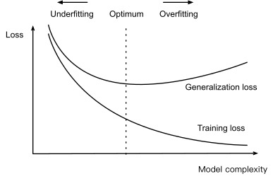
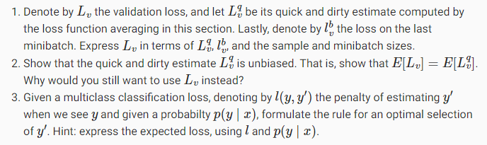
A higher-order polynomial function is more complex than a lower-order polynomial function, since the higher-order polynomial has more parameters and the model function’s selection range is wider. Fixing the training dataset, higher-order polynomial functions should always achieve lower (at worst, equal) training error relative to lower-degree polynomials. In fact, whenever each data example has a distinct value ofx, a polynomial function with degree equal to the number of data examples can fit the training set perfectly. We compare the relationship between polynomial degree (model complexity) and both underfitting and overfitting inFig. 3.6.1.
고차 다항식 함수는 저차 다항식 함수보다 더 복잡합니다. 왜냐하면 고차 다항식은 더 많은 매개변수를 갖고 모델 함수의 선택 범위가 더 넓기 때문입니다. 훈련 데이터 세트를 수정하면 고차 다항식 함수는 항상 저차 다항식에 비해 더 낮은(최악의 경우 동일한) 훈련 오류를 달성해야 합니다. 실제로 각 데이터 예제에 고유한 x 값이 있을 때마다 데이터 예제 수와 동일한 차수를 갖는 다항식 함수가 훈련 세트에 완벽하게 맞을 수 있습니다. 그림 3.6.1에서 다항식 차수(모델 복잡도)와 과소적합 및 과적합 간의 관계를 비교합니다.
Fig. 3.6.1 Influence of model complexity on underfitting and overfitting.
3.6.2.2.Dataset Siz
As the above bound already indicates, another big consideration to bear in mind is dataset size. Fixing our model, the fewer samples we have in the training dataset, the more likely (and more severely) we are to encounter overfitting. As we increase the amount of training data, the generalization error typically decreases. Moreover, in general, more data never hurts. For a fixed task and data distribution, model complexity should not increase more rapidly than the amount of data. Given more data, we might attempt to fit a more complex model. Absent sufficient data, simpler models may be more difficult to beat. For many tasks, deep learning only outperforms linear models when many thousands of training examples are available. In part, the current success of deep learning owes considerably to the abundance of massive datasets arising from Internet companies, cheap storage, connected devices, and the broad digitization of the economy.
위의 한계에서 이미 알 수 있듯이 염두에 두어야 할 또 다른 큰 고려 사항은 데이터 세트 크기입니다. 모델을 수정하면 훈련 데이터 세트에 있는 샘플 수가 줄어들수록 과적합이 발생할 가능성이 더 높아집니다(심각하게도). 훈련 데이터의 양을 늘리면 일반적으로 일반화 오류가 감소합니다. 또한 일반적으로 더 많은 데이터가 해를 끼치 지 않습니다. 고정된 작업 및 데이터 분포의 경우 모델 복잡성이 데이터 양보다 더 빠르게 증가해서는 안 됩니다. 더 많은 데이터가 주어지면 더 복잡한 모델을 맞추려고 시도할 수도 있습니다. 데이터가 충분하지 않으면 단순한 모델을 이기기가 더 어려울 수 있습니다. 많은 작업에서 딥 러닝은 수천 개의 학습 예제를 사용할 수 있는 경우에만 선형 모델보다 성능이 뛰어납니다. 부분적으로 현재 딥 러닝의 성공은 인터넷 회사, 저렴한 스토리지, 연결된 장치 및 경제의 광범위한 디지털화에서 발생하는 풍부한 대규모 데이터 세트에 크게 기인합니다.
3.6.3.Model Selection
Typically, we select our final model only after evaluating multiple models that differ in various ways (different architectures, training objectives, selected features, data preprocessing, learning rates, etc.). Choosing among many models is aptly calledmodel selection.
일반적으로 우리는 다양한 방식(다양한 아키텍처, 교육 목표, 선택한 기능, 데이터 전처리, 학습 속도 등)이 다른 여러 모델을 평가한 후에만 최종 모델을 선택합니다. 여러 모델 중에서 선택하는 것을 적절하게는 모델 선택이라고 합니다.
In principle, we should not touch our test set until after we have chosen all our hyperparameters. Were we to use the test data in the model selection process, there is a risk that we might overfit the test data. Then we would be in serious trouble. If we overfit our training data, there is always the evaluation on test data to keep us honest. But if we overfit the test data, how would we ever know? SeeOnget al.(2005)for an example of how this can lead to absurd results even for models where the complexity can be tightly controlled.
원칙적으로 모든 하이퍼파라미터를 선택할 때까지 테스트 세트를 건드리면 안 됩니다. 모델 선택 과정에서 테스트 데이터를 사용한다면 테스트 데이터에 과적합될 위험이 있습니다. 그러면 우리는 심각한 문제에 빠지게 될 것입니다. 훈련 데이터를 과대적합하는 경우 정직성을 유지하기 위해 항상 테스트 데이터에 대한 평가가 있습니다. 하지만 테스트 데이터에 과대적합되면 어떻게 알 수 있을까요? Ong et al. (2005)은 복잡성이 엄격하게 제어될 수 있는 모델의 경우에도 이것이 어떻게 터무니없는 결과로 이어질 수 있는지에 대한 예를 제공합니다.
Thus, we should never rely on the test data for model selection. And yet we cannot rely solely on the training data for model selection either because we cannot estimate the generalization error on the very data that we use to train the model.
따라서 모델 선택을 위해 테스트 데이터에 의존해서는 안 됩니다. 그러나 모델을 훈련하는 데 사용하는 바로 그 데이터에 대한 일반화 오류를 추정할 수 없기 때문에 모델 선택을 위해 훈련 데이터에만 의존할 수는 없습니다.
In practical applications, the picture gets muddier. While ideally we would only touch the test data once, to assess the very best model or to compare a small number of models with each other, real-world test data is seldom discarded after just one use. We can seldom afford a new test set for each round of experiments. In fact, recycling benchmark data for decades can have a significant impact on the development of algorithms, e.g., forimage classificationandoptical character recognition.
실제 적용에서는 그림이 더 흐릿해집니다. 이상적으로는 테스트 데이터를 한 번만 만지는 반면, 최고의 모델을 평가하거나 소수의 모델을 서로 비교하기 위해 실제 테스트 데이터는 한 번만 사용한 후 거의 삭제되지 않습니다. 우리는 각 실험 라운드마다 새로운 테스트 세트를 제공할 여력이 거의 없습니다. 실제로 수십 년 동안 벤치마크 데이터를 재활용하면 이미지 분류, 광학 문자 인식 등의 알고리즘 개발에 상당한 영향을 미칠 수 있습니다.
The common practice for addressing the problem oftraining on the test setis to split our data three ways, incorporating avalidation setin addition to the training and test datasets. The result is a murky business where the boundaries between validation and test data are worryingly ambiguous. Unless explicitly stated otherwise, in the experiments in this book we are really working with what should rightly be called training data and validation data, with no true test sets. Therefore, the accuracy reported in each experiment of the book is really the validation accuracy and not a true test set accuracy.
테스트 세트에 대한 교육 문제를 해결하기 위한 일반적인 방법은 데이터를 세 가지 방식으로 분할하고 교육 및 테스트 데이터세트 외에 검증 세트를 통합하는 것입니다. 그 결과 검증 데이터와 테스트 데이터 사이의 경계가 걱정스러울 정도로 모호한 비즈니스가 불투명해졌습니다. 달리 명시적으로 언급하지 않는 한, 이 책의 실험에서 우리는 실제 테스트 세트 없이 훈련 데이터와 검증 데이터라고 해야 할 것을 실제로 사용하고 있습니다. 따라서 책의 각 실험에서 보고된 정확도는 실제 검증 정확도이지 실제 테스트 세트 정확도가 아닙니다.
3.6.3.1.Cross-Validation
When training data is scarce, we might not even be able to afford to hold out enough data to constitute a proper validation set. One popular solution to this problem is to employK-fold cross-validation. Here, the original training data is split intoKnon-overlapping subsets. Then model training and validation are executedKtimes, each time training onK−1subsets and validating on a different subset (the one not used for training in that round). Finally, the training and validation errors are estimated by averaging over the results from the Kexperiments.
훈련 데이터가 부족하면 적절한 검증 세트를 구성하기에 충분한 데이터를 보유할 여력조차 없을 수도 있습니다. 이 문제에 대한 인기 있는 해결책 중 하나는 K-겹 교차 검증을 사용하는 것입니다. 여기서는 원본 훈련 데이터가 K개의 겹치지 않는 하위 집합으로 분할됩니다. 그런 다음 모델 훈련 및 검증이 K번 실행되며, 매번 K −1 하위 집합에 대해 훈련하고 다른 하위 집합(해당 라운드에서 훈련에 사용되지 않은 것)에 대해 검증합니다. 마지막으로 훈련 및 검증 오류는 K 실험 결과를 평균하여 추정됩니다.
3.6.4.Summary
This section explored some of the underpinnings of generalization in machine learning. Some of these ideas become complicated and counterintuitive when we get to deeper models; here, models are capable of overfitting data badly, and the relevant notions of complexity can be both implicit and counterintuitive (e.g., larger architectures with more parameters generalizing better). We leave you with a few rules of thumb:
이 섹션에서는 기계 학습에서 일반화의 몇 가지 토대를 살펴보았습니다. 이러한 아이디어 중 일부는 더 심층적인 모델에 도달하면 복잡해지고 직관에 반하게 됩니다. 여기서 모델은 데이터를 잘못 과적합할 수 있으며 관련 복잡성 개념은 암시적일 수도 있고 반직관적일 수도 있습니다(예: 더 많은 매개변수를 가진 더 큰 아키텍처가 더 잘 일반화됨). 몇 가지 경험 법칙을 알려드리겠습니다.
Use validation sets (orK-fold cross-validation) for model selection; 모델 선택을 위해 검증 세트(또는 K-겹 교차 검증)를 사용합니다.
More complex models often require more data; 더 복잡한 모델에는 더 많은 데이터가 필요한 경우가 많습니다.
Relevant notions of complexity include both the number of parameters and the range of values that they are allowed to take; 복잡성과 관련된 개념에는 매개변수의 수와 허용되는 값의 범위가 모두 포함됩니다.
Keeping all else equal, more data almost always leads to better generalization; 다른 모든 것을 동일하게 유지하면 더 많은 데이터가 거의 항상 더 나은 일반화로 이어집니다.
This entire talk of generalization is all predicated on the IID assumption. If we relax this assumption, allowing for distributions to shift between the train and testing periods, then we cannot say anything about generalization absent a further (perhaps milder) assumption. 일반화에 대한 이 전체 이야기는 모두 IID 가정에 근거합니다. 이 가정을 완화하여 열차와 테스트 기간 사이에 분포가 이동하도록 허용하면 추가(아마도 더 온화한) 가정 없이 일반화에 대해 아무 말도 할 수 없습니다.
3.6.5.Exercises
When can you solve the problem of polynomial regression exactly?
Give at least five examples where dependent random variables make treating the problem as IID data inadvisable.
Can you ever expect to see zero training error? Under which circumstances would you see zero generalization error?
Why isK-fold cross-validation very expensive to compute?
Why is theK-fold cross-validation error estimate biased?
The VC dimension is defined as the maximum number of points that can be classified with arbitrary labels{±1}by a function of a class of functions. Why might this not be a good idea for measuring how complex the class of functions is? Hint: consider the magnitude of the functions.
Your manager gives you a difficult dataset on which your current algorithm does not perform so well. How would you justify to him that you need more data? Hint: you cannot increase the data but you can decrease it.
In the previous sections, we worked through a number of hands-on applications of machine learning, fitting models to a variety of datasets. And yet, we never stopped to contemplate either where data comes from in the first place or what we plan to ultimately do with the outputs from our models. Too often, machine learning developers in possession of data rush to develop models without pausing to consider these fundamental issues.
이전 섹션에서는 기계 학습의 여러 hands-on applications -실습 응용 프로그램-을 통해 다양한 데이터 세트에 모델을 맞추었습니다. 그러나 우리는 처음부터 데이터가 어디에서 오는지 또는 궁극적으로 모델의 출력으로 무엇을 할 계획인지 고민하기 위한 시간을 충분히 갖지 않았습니다. 너무 자주 데이터를 소유한 기계 학습 개발자는 이러한 근본적인 문제를 고려하는것 보다 단지 모델을 개발하는 데만 몰두 합니다.
Many failed machine learning deployments can be traced back to this pattern. Sometimes models appear to perform marvelously as measured by test set accuracy but fail catastrophically in deployment when the distribution of data suddenly shifts. More insidiously, sometimes the very deployment of a model can be the catalyst that perturbs the data distribution. Say, for example, that we trained a model to predict who will repay vs. default on a loan, finding that an applicant’s choice of footwear was associated with the risk of default (Oxfords indicate repayment, sneakers indicate default). We might be inclined to thereafter grant loans to all applicants wearing Oxfords and to deny all applicants wearing sneakers.
실패한 많은 기계 학습 deployments -배포-는 이 패턴으로 거슬러 올라갈 수 있습니다. 때때로 모델은 테스트 세트 정확도로 측정했을 때 놀라운 성능을 보이는 것처럼 보이지만 데이터 분포가 갑자기 바뀌면 배치에서 치명적인 실패를 합니다. 더 은밀하게도 때로는 모델의 배포 자체가 데이터 분포를 교란시키는 촉매제가 될 수 있습니다. 예를 들어, 누가 상환할 것인지 채무불이행인지 예측하기 위해 모델을 훈련시켰고, 신청자의 신발 선택이 채무불이행 위험과 관련이 있다는 것을 발견했다고 가정해 보겠습니다(Oxfords는 상환을 나타내고 운동화는 채무불이행을 나타냅니다). 그 후 우리는 옥스퍼드를 신는 모든 지원자에게 대출을 허용하고 운동화를 신는 모든 지원자를 거부하는 경향이 있을 수 있습니다.
In this case, our ill-considered leap from pattern recognition to decision-making and our failure to critically consider the environment might have disastrous consequences. For starters, as soon as we began making decisions based on footwear, customers would catch on and change their behavior. Before long, all applicants would be wearing Oxfords, without any coinciding improvement in credit-worthiness. Take a minute to digest this because similar issues abound in many applications of machine learning: by introducing our model-based decisions to the environment, we might break the model.
이 경우 패턴 인식에서 의사 결정으로의 잘못된 도약과 환경을 비판적으로 고려하지 못하는 것은 재앙적인 결과를 초래할 수 있습니다. 우선, 우리가 신발을 기반으로 결정을 내리기 시작하자마자 고객은 그들의 행동을 파악하고 변화시킬 것입니다. 오래지 않아 모든 지원자들은 신용도가 향상되지 않은 채 옥스퍼드 구두를 신게 될 것입니다. 기계 학습의 많은 응용 프로그램에서 유사한 문제가 많기 때문에 잠시 시간을 내어 이를 이해하십시오. 모델 기반 결정을 환경에 도입하면 모델이 깨질 수 있습니다.
While we cannot possibly give these topics a complete treatment in one section, we aim here to expose some common concerns, and to stimulate the critical thinking required to detect these situations early, mitigate damage, and use machine learning responsibly. Some of the solutions are simple (ask for the “right” data), some are technically difficult (implement a reinforcement learning system), and others require that we step outside the realm of statistical prediction altogether and grapple with difficult philosophical questions concerning the ethical application of algorithms.
이러한 주제를 한 섹션에서 완전히 다룰 수는 없지만 여기서는 몇 가지 일반적인 우려 사항을 밝히고 이러한 상황을 조기에 감지하고 손상을 완화하며 기계 학습을 책임감 있게 사용하는 데 필요한 비판적 사고를 자극하는 것을 목표로 합니다. 솔루션 중 일부는 간단하고("올바른" 데이터 요청), 일부는 기술적으로 어렵고(강화 학습 시스템 구현), 다른 솔루션은 통계적 예측 영역을 완전히 벗어나 윤리적 문제에 관한 어려운 철학적 질문과 씨름해야 합니다. 알고리즘의 적용.
4.7.1.Types of Distribution Shift
To begin, we stick with the passive prediction setting considering the various ways that data distributions might shift and what might be done to salvage model performance. In one classic setup, we assume that our training data was sampled from some distribution ps(x,y)but that our test data will consist of unlabeled examples drawn from some different distributionpT(x,y). Already, we must confront a sobering reality. Absent any assumptions on howpsandprrelate to each other, learning a robust classifier is impossible.
시작하려면 데이터 분포가 이동할 수 있는 다양한 방식과 모델 성능을 복구하기 위해 수행할 수 있는 작업을 고려하여 수동 예측 설정을 고수합니다. 하나의 고전적인 설정에서 훈련 데이터는 일부 분포 ps(x,y)에서 샘플링되었지만 테스트 데이터는 일부 다른 분포 pT(x,y)에서 가져온 레이블이 지정되지 않은 예제로 구성된다고 가정합니다. 이미 우리는 냉정한 현실에 직면해야 합니다. ps와 pr이 서로 어떻게 관련되어 있는지에 대한 가정이 없으면 강력한 분류기를 학습하는 것은 불가능합니다.
Consider a binary classification problem, where we wish to distinguish between dogs and cats. If the distribution can shift in arbitrary ways, then our setup permits the pathological case in which the distribution over inputs remains constant:ps(x)=pr(x), but the labels are all flipped:ps(y∣x)=1−pT(y∣x). In other words, if God can suddenly decide that in the future all “cats” are now dogs and what we previously called “dogs” are now cats—without any change in the distribution of inputsp(d), then we cannot possibly distinguish this setting from one in which the distribution did not change at all.
개와 고양이를 구별하려는 이진 분류 문제를 고려하십시오. 분포가 임의의 방식으로 이동할 수 있는 경우, 우리의 설정은 입력에 대한 분포가 일정하게 유지되는 병리학적 사례를 허용합니다: ps(x)=pr(x), 그러나 레이블은 모두 뒤집힙니다: ps(y∣x)=1 -pT(y∣x). 다시 말해서, 입력 p(d)의 분포에 어떤 변화도 없이 신이 미래에 모든 "고양이"는 이제 개이고 우리가 이전에 "개"라고 불렀던 것은 이제 고양이라고 갑자기 결정할 수 있다면, 우리는 아마도 구별할 수 없습니다. 이 설정은 배포가 전혀 변경되지 않은 설정입니다.
Fortunately, under some restricted assumptions on the ways our data might change in the future, principled algorithms can detect shift and sometimes even adapt on the fly, improving on the accuracy of the original classifier.
다행스럽게도 미래에 데이터가 변경될 수 있는 방식에 대한 제한된 가정 하에서 원칙적 알고리즘은 이동을 감지하고 때로는 즉석에서 적응하여 원래 분류기의 정확도를 향상시킬 수 있습니다.
4.7.1.1.Covariate Shift
Among categories of distribution shift, covariate shift may be the most widely studied. Here, we assume that while the distribution of inputs may change over time, the labeling function, i.e., the conditional distributionP(y∣x)does not change. Statisticians call thiscovariate shiftbecause the problem arises due to a shift in the distribution of the covariates (features). While we can sometimes reason about distribution shift without invoking causality, we note that covariate shift is the natural assumption to invoke in settings where we believe thatxcausesy.
distribution shift-분포 이동-의 범주 중에서 covariateshift -공변량 이동-이 가장 널리 연구될 수 있습니다. 여기서는 distribution of inputs -입력 분포-가 시간에 따라 변할 수 있지만 labeling function-레이블링 함수-, 즉 conditional distribution-조건부 분포- P(y∣x)는 변하지 않는다고 가정합니다. 통계학자들은 covariates (features)-공변량(특징)- 분포의 변화로 인해 문제가 발생하기 때문에 이를 covariate shift -공변량 변화-라고 부릅니다. 우리는 때때로 인과 관계 없이 distribution shift-분포 이동-에 대해 추론할 수 있지만, covariate shift-공변량 이동-은 x가 y를 유발한다고 믿는 환경에서 호출하는 자연스러운 가정이라는 점에 주목합니다.
Consider the challenge of distinguishing cats and dogs. Our training data might consist of images of the kind inFig. 4.7.1.
고양이와 개를 구별하는 문제를 생각해 보십시오. 훈련 데이터는 그림 4.7.1과 같은 종류의 이미지로 구성될 수 있습니다.
At test time we are asked to classify the images inFig. 4.7.2.
테스트 할 때 그림 4.7.2의 이미지를 분류하라는 요청을 받았습니다.
The training set consists of photos, while the test set contains only cartoons. Training on a dataset with substantially different characteristics from the test set can spell trouble absent a coherent plan for how to adapt to the new domain.
훈련 세트는 사진으로 구성되고 테스트 세트는 만화로만 구성됩니다. 테스트 세트와 상당히 다른 특성을 가진 데이터 세트에 대한 교육은 새로운 도메인에 적응하는 방법에 대한 일관된 계획이 없을 수 있습니다.
4.7.1.2.Label Shift
Label shiftdescribes the converse problem. Here, we assume that the label marginal P(y)can change but the class-conditional distributionP(x∣y)remains fixed across domains. Label shift is a reasonable assumption to make when we believe thatycausesx. For example, we may want to predict diagnoses given their symptoms (or other manifestations), even as the relative prevalence of diagnoses are changing over time. Label shift is the appropriate assumption here because diseases cause symptoms. In some degenerate cases the label shift and covariate shift assumptions can hold simultaneously. For example, when the label is deterministic, the covariate shift assumption will be satisfied, even whenycausesx. Interestingly, in these cases, it is often advantageous to work with methods that flow from the label shift assumption. That is because these methods tend to involve manipulating objects that look like labels (often low-dimensional), as opposed to objects that look like inputs, which tend to be high-dimensional in deep learning.
레이블 이동은 반대 문제를 설명합니다. 여기에서 레이블 한계 P(y)는 변경될 수 있지만 클래스 조건부 분포 P(x∣y)는 도메인 전체에서 고정된 상태로 유지된다고 가정합니다. 레이블 이동은 y가 x를 유발한다고 믿을 때 합리적인 가정입니다. 예를 들어, 진단의 상대적 유병률이 시간이 지남에 따라 변하더라도 증상(또는 다른 징후)에 따라 진단을 예측할 수 있습니다. 질병이 증상을 유발하기 때문에 레이블 이동이 적절한 가정입니다. 일부 변질된 경우에는 레이블 이동 및 공변량 이동 가정이 동시에 유지될 수 있습니다. 예를 들어 레이블이 결정적이면 y가 x를 유발하는 경우에도 공변량 이동 가정이 충족됩니다. 흥미롭게도 이러한 경우 레이블 이동 가정에서 파생된 방법으로 작업하는 것이 종종 유리합니다. 이러한 방법은 딥 러닝에서 고차원 경향이 있는 입력처럼 보이는 개체와 달리 레이블(종종 저차원)처럼 보이는 개체를 조작하는 경향이 있기 때문입니다.
4.7.1.3.Concept Shift
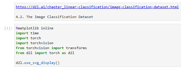
We may also encounter the related problem ofconcept shift, which arises when the very definitions of labels can change. This sounds weird—acatis acat, no? However, other categories are subject to changes in usage over time. Diagnostic criteria for mental illness, what passes for fashionable, and job titles, are all subject to considerable amounts of concept shift. It turns out that if we navigate around the United States, shifting the source of our data by geography, we will find considerable concept shift regarding the distribution of names forsoft drinksas shown inFig. 4.7.3.
또한 레이블의 정의가 변경될 수 있을 때 발생하는 개념 이동과 관련된 문제에 직면할 수 있습니다. 이상하게 들립니다. 고양이는 고양이잖아요? 그러나 다른 범주는 시간이 지남에 따라 사용량이 변경될 수 있습니다. 정신 질환에 대한 진단 기준, 유행에 통하는 것, 직책은 모두 상당한 양의 개념 변화를 겪습니다. 우리가 미국을 돌아다니면서 지역별로 데이터 소스를 이동하면 그림 4.7.3에 표시된 것처럼 청량 음료의 이름 분포와 관련하여 상당한 개념 변화가 있음을 알 수 있습니다.
Fig. 4.7.3 Concept shift on soft drink names in the United States.
If we were to build a machine translation system, the distributionP(y∣x)might be different depending on our location. This problem can be tricky to spot. We might hope to exploit knowledge that shift only takes place gradually either in a temporal or geographic sense.
기계 번역 시스템을 구축한다면 위치에 따라 분포 P(y∣x)가 다를 수 있습니다. 이 문제는 파악하기 까다로울 수 있습니다. 우리는 변화가 시간적 또는 지리적 의미에서 점진적으로만 발생한다는 지식을 활용하기를 희망할 수 있습니다.
4.7.2.Examples of Distribution Shift
형식주의와 알고리즘을 탐구하기 전에 공변량 또는 개념 이동이 명확하지 않을 수 있는 몇 가지 구체적인 상황에 대해 논의할 수 있습니다.
4.7.2.1.Medical Diagnostics
Imagine that you want to design an algorithm to detect cancer. You collect data from healthy and sick people and you train your algorithm. It works fine, giving you high accuracy and you conclude that you are ready for a successful career in medical diagnostics.Not so fast.
암을 감지하는 알고리즘을 설계한다고 상상해 보십시오. 건강하고 아픈 사람들로부터 데이터를 수집하고 알고리즘을 훈련합니다. 그것은 잘 작동하고 높은 정확도를 제공하며 의료 진단 분야에서 성공적인 경력을 쌓을 준비가 되었다고 결론을 내립니다. 그렇게 빠르지 않습니다.
The distributions that gave rise to the training data and those you will encounter in the wild might differ considerably. This happened to an unfortunate startup that some of us (authors) worked with years ago. They were developing a blood test for a disease that predominantly affects older men and hoped to study it using blood samples that they had collected from patients. However, it is considerably more difficult to obtain blood samples from healthy men than sick patients already in the system. To compensate, the startup solicited blood donations from students on a university campus to serve as healthy controls in developing their test. Then they asked whether we could help them to build a classifier for detecting the disease.
훈련 데이터를 생성한 분포와 실제로 접하게 될 분포는 상당히 다를 수 있습니다. 이것은 우리 중 일부(저자)가 몇 년 전에 함께 일했던 불행한 시작에 일어났습니다. 그들은 주로 노인에게 영향을 미치는 질병에 대한 혈액 검사를 개발하고 있었고 환자로부터 수집한 혈액 샘플을 사용하여 연구하기를 희망했습니다. 그러나 이미 시스템에 있는 아픈 환자보다 건강한 남성에게서 혈액 샘플을 채취하는 것이 훨씬 더 어렵습니다. 이를 보완하기 위해 이 스타트업은 대학 캠퍼스의 학생들에게 헌혈을 요청하여 테스트를 개발하는 데 있어 건강한 통제 역할을 했습니다. 그런 다음 그들은 질병을 감지하기 위한 분류기를 구축하는 데 도움을 줄 수 있는지 물었습니다.
As we explained to them, it would indeed be easy to distinguish between the healthy and sick cohorts with near-perfect accuracy. However, that is because the test subjects differed in age, hormone levels, physical activity, diet, alcohol consumption, and many more factors unrelated to the disease. This was unlikely to be the case with real patients. Due to their sampling procedure, we could expect to encounter extreme covariate shift. Moreover, this case was unlikely to be correctable via conventional methods. In short, they wasted a significant sum of money.
우리가 그들에게 설명했듯이 거의 완벽에 가까운 정확도로 건강한 코호트와 아픈 코호트를 쉽게 구별할 수 있습니다. 그러나 이는 피험자들의 연령, 호르몬 수치, 신체 활동, 식이요법, 알코올 소비 및 질병과 관련 없는 더 많은 요인이 다르기 때문입니다. 이것은 실제 환자의 경우가 아닐 것입니다. 샘플링 절차로 인해 극단적인 공변량 이동이 발생할 것으로 예상할 수 있습니다. 게다가 이 경우는 기존의 방법으로는 교정할 수 없었습니다. 요컨대, 그들은 상당한 양의 돈을 낭비했습니다.
4.7.2.2.Self-Driving Cars
Say a company wanted to leverage machine learning for developing self-driving cars. One key component here is a roadside detector. Since real annotated data is expensive to get, they had the (smart and questionable) idea to use synthetic data from a game rendering engine as additional training data. This worked really well on “test data” drawn from the rendering engine. Alas, inside a real car it was a disaster. As it turned out, the roadside had been rendered with a very simplistic texture. More importantly,allthe roadside had been rendered with thesametexture and the roadside detector learned about this “feature” very quickly.
회사에서 자율 주행 자동차 개발을 위해 머신 러닝을 활용하고자 한다고 가정해 보겠습니다. 여기서 핵심 구성 요소 중 하나는 길가 감지기입니다. 주석이 달린 실제 데이터를 얻는 데 비용이 많이 들기 때문에 그들은 게임 렌더링 엔진의 합성 데이터를 추가 교육 데이터로 사용하는 (현명하고 의심스러운) 아이디어를 가졌습니다. 이것은 렌더링 엔진에서 가져온 "테스트 데이터"에서 정말 잘 작동했습니다. 아아, 실제 차 안에서는 재앙이었습니다. 결과적으로 길가는 매우 단순한 질감으로 렌더링되었습니다. 더 중요한 것은 모든 길가가 동일한 텍스처로 렌더링되었고 길가 탐지기가 이 "기능"에 대해 매우 빠르게 학습했다는 것입니다.
A similar thing happened to the US Army when they first tried to detect tanks in the forest. They took aerial photographs of the forest without tanks, then drove the tanks into the forest and took another set of pictures. The classifier appeared to workperfectly. Unfortunately, it had merely learned how to distinguish trees with shadows from trees without shadows—the first set of pictures was taken in the early morning, the second set at noon.
미군이 처음 숲에서 탱크를 탐지하려 했을 때 비슷한 일이 일어났습니다. 그들은 탱크가 없는 숲의 항공 사진을 찍은 다음 탱크를 숲으로 몰고 또 다른 사진을 찍었습니다. 분류기는 완벽하게 작동하는 것으로 나타났습니다. 안타깝게도 그림자가 있는 나무와 그림자가 없는 나무를 구별하는 방법을 배웠을 뿐이었습니다. 첫 번째 사진 세트는 이른 아침에, 두 번째 세트는 정오에 촬영했습니다.
4.7.2.3.Nonstationary Distributions
A much more subtle situation arises when the distribution changes slowly (also known asnonstationary distribution) and the model is not updated adequately. Below are some typical cases.
분포가 느리게 변경되고(비정상 분포라고도 함) 모델이 적절하게 업데이트되지 않는 경우 훨씬 더 미묘한 상황이 발생합니다. 다음은 몇 가지 일반적인 경우입니다.
We train a computational advertising model and then fail to update it frequently (e.g., we forget to incorporate that an obscure new device called an iPad was just launched). 우리는 전산 광고 모델을 훈련한 다음 자주 업데이트하지 않습니다(예: iPad라는 모호한 새 장치가 방금 출시되었다는 사실을 통합하는 것을 잊었습니다).
We build a spam filter. It works well at detecting all spam that we have seen so far. But then the spammers wisen up and craft new messages that look unlike anything we have seen before. 우리는 스팸 필터를 만듭니다. 지금까지 본 모든 스팸을 탐지하는 데 효과적입니다. 그러나 스패머는 정신을 차리고 우리가 이전에 본 것과는 전혀 다른 새로운 메시지를 만듭니다.
We build a product recommendation system. It works throughout the winter but then continues to recommend Santa hats long after Christmas. 상품 추천 시스템을 구축합니다. 그것은 겨울 내내 작동하지만 크리스마스 이후에도 계속해서 산타 모자를 추천합니다.
4.7.2.4.More Anecdotes
We build a face detector. It works well on all benchmarks. Unfortunately it fails on test data—the offending examples are close-ups where the face fills the entire image (no such data was in the training set). 우리는 얼굴 검출기를 만듭니다. 모든 벤치마크에서 잘 작동합니다. 안타깝게도 테스트 데이터에서는 실패했습니다. 불쾌한 예는 얼굴이 전체 이미지를 채우는 클로즈업입니다(트레이닝 세트에는 그러한 데이터가 없었습니다).
We build a Web search engine for the US market and want to deploy it in the UK. 우리는 미국 시장을 위한 웹 검색 엔진을 구축하고 영국에 배포하려고 합니다.
We train an image classifier by compiling a large dataset where each among a large set of classes is equally represented in the dataset, say 1000 categories, represented by 1000 images each. Then we deploy the system in the real world, where the actual label distribution of photographs is decidedly non-uniform. 우리는 각각 1000개의 이미지로 표시되는 1000개의 범주와 같이 큰 클래스 세트 중 각각이 데이터 세트에서 동일하게 표현되는 큰 데이터 세트를 컴파일하여 이미지 분류기를 훈련합니다. 그런 다음 사진의 실제 레이블 배포가 확실히 균일하지 않은 실제 세계에 시스템을 배포합니다.
4.7.3.Correction of Distribution Shift
As we have discussed, there are many cases where training and test distributionsP(x,y)are different. In some cases, we get lucky and the models work despite covariate, label, or concept shift. In other cases, we can do better by employing principled strategies to cope with the shift. The remainder of this section grows considerably more technical. The impatient reader could continue on to the next section as this material is not prerequisite to subsequent concepts.
논의한 바와 같이 훈련 및 테스트 분포 P(x,y)가 다른 경우가 많습니다. 어떤 경우에는 운이 좋아 공변량, 레이블 또는 개념 이동에도 불구하고 모델이 작동합니다. 다른 경우에는 변화에 대처하기 위해 원칙에 입각한 전략을 사용함으로써 더 잘할 수 있습니다. 이 섹션의 나머지 부분은 훨씬 더 기술적으로 성장합니다. 이 자료는 후속 개념의 전제 조건이 아니므로 참을성 없는 독자는 다음 섹션으로 계속 진행할 수 있습니다.
4.7.3.1.Empirical Risk and Risk
Let’s first reflect about what exactly is happening during model training: we iterate over features and associated labels of training data{(x1,y1),…,(xn,yn)}and update the parameters of a modelfafter every minibatch. For simplicity we do not consider regularization, so we largely minimize the loss on the training:
먼저 모델 학습 중에 정확히 어떤 일이 발생하는지 살펴보겠습니다. 학습 데이터 {(x1,y1),… 단순화를 위해 정규화를 고려하지 않으므로 교육 손실을 크게 최소화합니다.
wherelis the loss function measuring “how bad” the predictionf(xi)is given the associated labelyi. Statisticians call the term in(4.7.1)empirical risk. Theempirical riskis an average loss over the training data to approximate therisk, which is the expectation of the loss over the entire population of data drawn from their true distributionp(x,y):
여기서 l은 "얼마나 나쁜지"를 측정하는 손실 함수입니다. 예측 f(xi)에는 관련 레이블 yi가 지정됩니다. 통계학자들은 이 용어를 (4.7.1) 경험적 위험이라고 부릅니다. 경험적 위험은 실제 분포 p(x,y)에서 가져온 전체 데이터 모집단에 대한 손실의 예상인 위험을 근사화하기 위한 훈련 데이터에 대한 평균 손실입니다.
However, in practice we typically cannot obtain the entire population of data. Thus,empirical risk minimization, which is minimizing the empirical risk in(4.7.1), is a practical strategy for machine learning, with the hope to approximate minimizing the risk.
그러나 실제로는 일반적으로 전체 데이터 모집단을 얻을 수 없습니다. 따라서 (4.7.1)에서 경험적 위험을 최소화하는 경험적 위험 최소화는 위험 최소화에 근접하기를 희망하는 기계 학습을 위한 실용적인 전략입니다.
4.7.3.2.Covariate Shift Correction
Assume that we want to estimate some dependencyP(y∣x)for which we have labeled data(xi,yi). Unfortunately, the observationsxiare drawn from somesource distributionq(x)rather than thetarget distributionp(x). Fortunately, the dependency assumption means that the conditional distribution does not change:p(y∣x)=q(y∣x). If the source distributionq(x)is “wrong”, we can correct for that by using the following simple identity in the risk:
레이블이 지정된 데이터(xi,yi)에 대한 일부 종속성 P(y∣x)를 추정하려고 한다고 가정합니다. 불행하게도 관측값 xi는 목표 분포 p(x)가 아닌 일부 소스 분포 q(x)에서 가져옵니다. 다행스럽게도 종속성 가정은 조건부 분포가 변경되지 않음을 의미합니다: p(y∣x)=q(y∣x). 소스 분포 q(x)가 "잘못된" 경우 위험에서 다음과 같은 간단한 ID를 사용하여 이를 수정할 수 있습니다.
In other words, we need to reweigh each data example by the ratio of the probability that it would have been drawn from the correct distribution to that from the wrong one:
즉, 올바른 분포에서 도출된 확률과 잘못된 분포에서 도출된 확률의 비율로 각 데이터 예제를 다시 평가해야 합니다.
Plugging in the weightBifor each data example(xi,yi)we can train our model usingweighted empirical risk minimization:
각 데이터 예(xi,yi)에 가중치 Bi를 연결하면 가중 경험적 위험 최소화를 사용하여 모델을 훈련할 수 있습니다.
Alas, we do not know that ratio, so before we can do anything useful we need to estimate it. Many methods are available, including some fancy operator-theoretic approaches that attempt to recalibrate the expectation operator directly using a minimum-norm or a maximum entropy principle. Note that for any such approach, we need samples drawn from both distributions—the “true”p, e.g., by access to test data, and the one used for generating the training setq(the latter is trivially available). Note however, that we only need featuresx∼p(x); we do not need to access labelsy∼p(y).
아아, 우리는 그 비율을 모르기 때문에 유용한 일을 하기 전에 그것을 추정해야 합니다. 최소 표준 또는 최대 엔트로피 원리를 사용하여 기대 연산자를 직접 재조정하려는 멋진 연산자 이론적 접근 방식을 포함하여 많은 방법을 사용할 수 있습니다. 이러한 접근 방식의 경우 테스트 데이터에 대한 액세스와 같은 "참" p와 훈련 세트 q를 생성하는 데 사용되는 분포(후자는 쉽게 사용할 수 있음)의 두 분포에서 추출한 샘플이 필요합니다. 그러나 특징 x~p(x)만 필요하다는 점에 유의하십시오. 레이블 y~p(y)에 액세스할 필요가 없습니다.
In this case, there exists a very effective approach that will give almost as good results as the original: logistic regression, which is a special case of softmax regression (seeSection 4.1) for binary classification. This is all that is needed to compute estimated probability ratios. We learn a classifier to distinguish between data drawn fromp(x)and data drawn fromq(x). If it is impossible to distinguish between the two distributions then it means that the associated instances are equally likely to come from either one of the two distributions. On the other hand, any instances that can be well discriminated should be significantly overweighted or underweighted accordingly.
이 경우 원본과 거의 동일한 결과를 제공하는 매우 효과적인 접근 방식이 존재합니다. 로지스틱 회귀는 이진 분류에 대한 소프트맥스 회귀(섹션 4.1 참조)의 특수한 경우입니다. 이것이 추정 확률 비율을 계산하는 데 필요한 전부입니다. 우리는 p(x)에서 가져온 데이터와 q(x)에서 가져온 데이터를 구별하기 위해 분류기를 배웁니다. 두 분포를 구별하는 것이 불가능하다면 연결된 인스턴스가 두 분포 중 하나에서 나올 가능성이 동일하다는 의미입니다. 반면에 잘 식별할 수 있는 인스턴스는 그에 따라 크게 과중되거나 과소되어야 합니다.
For simplicity’s sake assume that we have an equal number of instances from both distributionsp(x)andq(x), respectively. Now denote byzlabels that are1for data drawn frompand−1for data drawn fromq. Then the probability in a mixed dataset is given by
단순화를 위해 분포 p(x) 및 q(x) 각각에서 동일한 수의 인스턴스가 있다고 가정합니다. 이제 p에서 가져온 데이터의 경우 1이고 q에서 가져온 데이터의 경우 -1인 z 레이블로 표시합니다. 그런 다음 혼합 데이터 세트의 확률은 다음과 같이 지정됩니다.
Thus, if we use a logistic regression approach, whereP(z=1∣x)=1/1+exp(−ℎ(x))(ℎis a parameterized function), it follows that
따라서 P(z=1∣x)=1/1+exp(−ℎ(x))(ℎ는 매개변수화된 함수임)인 로지스틱 회귀 접근법을 사용하면 다음과 같이 됩니다.
As a result, we need to solve two problems: first one to distinguish between data drawn from both distributions, and then a weighted empirical risk minimization problem in(4.7.5)where we weigh terms byBi.
결과적으로 우리는 두 가지 문제를 해결해야 합니다. 첫 번째 문제는 두 분포에서 가져온 데이터를 구별하는 것입니다. 그런 다음 Bi로 용어를 평가하는 (4.7.5)의 가중 경험적 위험 최소화 문제입니다.
Now we are ready to describe a correction algorithm. Suppose that we have a training set{(x1,y1),…,(xn,yn)}and an unlabeled test set{u1,…,um}. For covariate shift, we assume thatxifor all1 ≤ i ≤ nare drawn from some source distribution anduifor all1 ≤ i ≤ mare drawn from the target distribution. Here is a prototypical algorithm for correcting covariate shift:
이제 보정 알고리즘을 설명할 준비가 되었습니다. 트레이닝 세트 {(x1,y1),…,(xn,yn)}와 레이블이 지정되지 않은 테스트 세트 {u1,…,um}이 있다고 가정합니다. 공변량 이동의 경우 모든 1 ≤ i ≤ n에 대한 xi는 일부 소스 분포에서 도출되고 모든 1 ≤ i ≤ m에 대한 ui는 대상 분포에서 도출된다고 가정합니다. 다음은 공변량 이동을 수정하기 위한 원형 알고리즘입니다.
Generate a binary-classification training set:{(x1,−1),…,(xn,−1),(u1,1),…,(um,1)}.
Train a binary classifier using logistic regression to get functionℎ.
Weigh training data usingBi=exp(ℎ(xi))or betterBi=min(exp(ℎ(xi)),c)for some constantc.
Use weightsBifor training on{(x1,y1),…,(xn,yn)}in(4.7.5).
Note that the above algorithm relies on a crucial assumption. For this scheme to work, we need that each data example in the target (e.g., test time) distribution had nonzero probability of occurring at training time. If we find a point wherep(x)>0butq(x)=0, then the corresponding importance weight should be infinity.
위의 알고리즘은 중요한 가정에 의존합니다. 이 체계가 작동하려면 대상(예: 테스트 시간) 분포의 각 데이터 예제가 훈련 시간에 발생할 확률이 0이 아니어야 합니다. p(x)>0이지만 q(x)=0인 점을 찾으면 해당 중요도 가중치는 무한대여야 합니다.
4.7.3.3.Label Shift Correction
Assume that we are dealing with a classification task withkcategories. Using the same notation inSection 4.7.3.2,qandpare the source distribution (e.g., training time) and target distribution (e.g., test time), respectively. Assume that the distribution of labels shifts over time:q(y)≠p(y), but the class-conditional distribution stays the same:q(x∣y)=p(x∣y). If the source distributionq(y)is “wrong”, we can correct for that according to the following identity in the risk as defined in(4.7.2):
k개의 범주로 분류 작업을 처리한다고 가정합니다. 섹션 4.7.3.2의 동일한 표기법을 사용하여 q 및 p는 각각 소스 분포(예: 교육 시간) 및 대상 분포(예: 테스트 시간)입니다. 레이블 분포는 시간이 지남에 따라 이동한다고 가정합니다: q(y)≠p(y). 그러나 클래스 조건부 분포는 동일하게 유지됩니다: q(x∣y)=p(x∣y). 소스 분포 q(y)가 "잘못된" 경우 (4.7.2)에 정의된 위험의 다음 ID에 따라 이를 수정할 수 있습니다.
Here, our importance weights will correspond to the label likelihood ratios
여기서 중요도 가중치는 레이블 우도 비율에 해당합니다.
One nice thing about label shift is that if we have a reasonably good model on the source distribution, then we can get consistent estimates of these weights without ever having to deal with the ambient dimension. In deep learning, the inputs tend to be high-dimensional objects like images, while the labels are often simpler objects like categories.
레이블 이동에 대한 한 가지 좋은 점은 소스 분포에 대해 상당히 좋은 모델이 있는 경우 주변 차원을 처리하지 않고도 이러한 가중치의 일관된 추정치를 얻을 수 있다는 것입니다. 딥 러닝에서 입력은 이미지와 같은 고차원 개체인 경향이 있는 반면 레이블은 범주와 같은 단순한 개체인 경우가 많습니다.
To estimate the target label distribution, we first take our reasonably good off-the-shelf classifier (typically trained on the training data) and compute its confusion matrix using the validation set (also from the training distribution). Theconfusion matrix,C, is simply ak×kmatrix, where each column corresponds to the label category (ground truth) and each row corresponds to our model’s predicted category. Each cell’s valuecijis the fraction of total predictions on the validation set where the true label wasjand our model predictedi.
대상 레이블 분포를 추정하기 위해 먼저 합리적으로 우수한 기성 분류기(일반적으로 훈련 데이터에 대해 훈련됨)를 선택하고 유효성 검사 세트(역시 훈련 분포에서)를 사용하여 혼동 행렬을 계산합니다. 혼동 행렬 C는 단순히 k×k 행렬이며 각 열은 레이블 범주(실측 정보)에 해당하고 각 행은 모델의 예측 범주에 해당합니다. 각 셀의 값 cij는 실제 레이블이 j이고 모델이 i를 예측한 검증 세트에 대한 총 예측의 비율입니다.
Now, we cannot calculate the confusion matrix on the target data directly, because we do not get to see the labels for the examples that we see in the wild, unless we invest in a complex real-time annotation pipeline. What we can do, however, is average all of our models predictions at test time together, yielding the mean model outputsu(y^)∈Rk, whoseithelementu(y^i)is the fraction of total predictions on the test set where our model predictedi.
이제는 복잡한 실시간 주석 파이프라인에 투자하지 않는 한 야생에서 보는 예제에 대한 레이블을 볼 수 없기 때문에 대상 데이터에 대한 혼동 행렬을 직접 계산할 수 없습니다. 그러나 우리가 할 수 있는 것은 테스트 시간에 모든 모델 예측을 함께 평균화하여 평균 모델 출력 u(y^)∈Rk를 산출하는 것입니다. 여기서 i번째 요소 u(y^i)는 테스트에 대한 총 예측의 비율입니다. 모델이 i를 예측한 위치를 설정합니다.
It turns out that under some mild conditions—if our classifier was reasonably accurate in the first place, and if the target data contains only categories that we have seen before, and if the label shift assumption holds in the first place (the strongest assumption here), then we can estimate the test set label distribution by solving a simple linear system
일부 온화한 조건에서 분류기가 처음부터 합리적으로 정확하고 대상 데이터에 이전에 본 범주만 포함되어 있고 레이블 이동 가정이 처음에 유지되는 경우(여기서 가장 강력한 가정은 ) 그런 다음 간단한 선형 시스템을 해결하여 테스트 세트 레이블 분포를 추정할 수 있습니다.
because as an estimate∑k j=1cijP(yj)=u(y^i)holds for all1≤ i ≤ k, wherep(yj)is thej thelement of thek-dimensional label distribution vectorp(y). If our classifier is sufficiently accurate to begin with, then the confusion matrixCwill be invertible, and we get a solutionp(y)=C−1u(y^).
추정치로서 ∑k j=1cijP(yj)=u(y^i)는 모든 1≤ i ≤ k에 대해 유지되며, 여기서 p(yj)는 k차원 레이블 분포 벡터 p(y)의 j 번째 요소입니다. 분류기가 시작하기에 충분히 정확하다면 혼동 행렬 C는 가역적이며 솔루션 p(y)=C−1u(y^)를 얻습니다.
Because we observe the labels on the source data, it is easy to estimate the distributionq(y). Then for any training exampleiwith labelyi, we can take the ratio of our estimatedp(yi)/q(yi)to calculate the weightBi, and plug this into weighted empirical risk minimization in(4.7.5).
Concept shift is much harder to fix in a principled manner. For instance, in a situation where suddenly the problem changes from distinguishing cats from dogs to one of distinguishing white from black animals, it will be unreasonable to assume that we can do much better than just collecting new labels and training from scratch. Fortunately, in practice, such extreme shifts are rare. Instead, what usually happens is that the task keeps on changing slowly. To make things more concrete, here are some examples:
개념 전환은 원칙적으로 수정하기가 훨씬 더 어렵습니다. 예를 들어, 문제가 고양이와 개를 구별하는 것에서 흰색과 검은색 동물을 구별하는 것으로 갑자기 바뀌는 상황에서 우리가 새 레이블을 수집하고 처음부터 훈련하는 것보다 훨씬 더 잘할 수 있다고 가정하는 것은 비합리적입니다. 다행스럽게도 실제로 이러한 극단적인 변화는 드뭅니다. 대신 일반적으로 발생하는 일은 작업이 계속해서 느리게 변경된다는 것입니다. 좀 더 구체적으로 설명하자면 다음과 같은 몇 가지 예입니다.
In computational advertising, new products are launched, old products become less popular. This means that the distribution over ads and their popularity changes gradually and any click-through rate predictor needs to change gradually with it.
전산 광고에서는 신제품이 출시되고 오래된 제품은 인기가 떨어집니다. 즉, 광고에 대한 분포와 그 인기도가 점진적으로 변하고 모든 클릭률 예측기가 그에 따라 점진적으로 변해야 함을 의미합니다.
Traffic camera lenses degrade gradually due to environmental wear, affecting image quality progressively.
교통 카메라 렌즈는 환경적 마모로 인해 점진적으로 저하되어 이미지 품질에 점진적으로 영향을 미칩니다.
News content changes gradually (i.e., most of the news remains unchanged but new stories appear).
뉴스 콘텐츠는 점진적으로 변경됩니다(즉, 대부분의 뉴스는 변경되지 않지만 새로운 기사가 나타남).
In such cases, we can use the same approach that we used for training networks to make them adapt to the change in the data. In other words, we use the existing network weights and simply perform a few update steps with the new data rather than training from scratch.
이러한 경우 네트워크 훈련에 사용한 것과 동일한 접근 방식을 사용하여 데이터의 변화에 적응할 수 있습니다. 즉, 우리는 기존 네트워크 가중치를 사용하고 처음부터 훈련하는 대신 새 데이터로 몇 가지 업데이트 단계를 수행합니다.
4.7.4.A Taxonomy of Learning Problems
Armed with knowledge about how to deal with changes in distributions, we can now consider some other aspects of machine learning problem formulation.
분포의 변화를 다루는 방법에 대한 지식으로 무장한 우리는 이제 기계 학습 문제 공식화의 다른 측면을 고려할 수 있습니다.
4.7.4.1.Batch Learning
Inbatch learning, we have access to training features and labels{(x1,y1),…,(xn,yn)}, which we use to train a modelf(x). Later on, we deploy this model to score new data(x,y)drawn from the same distribution. This is the default assumption for any of the problems that we discuss here. For instance, we might train a cat detector based on lots of pictures of cats and dogs. Once we trained it, we ship it as part of a smart catdoor computer vision system that lets only cats in. This is then installed in a customer’s home and is never updated again (barring extreme circumstances).
배치 학습에서는 모델 f(x)를 훈련하는 데 사용하는 훈련 기능 및 레이블 {(x1,y1),…,(xn,yn)}에 액세스할 수 있습니다. 나중에 이 모델을 배포하여 동일한 분포에서 가져온 새 데이터(x,y)의 점수를 매깁니다. 이것은 여기서 논의하는 모든 문제에 대한 기본 가정입니다. 예를 들어 많은 고양이와 개 사진을 기반으로 고양이 감지기를 훈련시킬 수 있습니다. 훈련을 마치면 고양이만 들어올 수 있는 스마트 캣도어 컴퓨터 비전 시스템의 일부로 배송합니다. 그런 다음 고객의 집에 설치되고 다시는 업데이트되지 않습니다(극단적인 상황 제외).
4.7.4.2.Online Learning
Now imagine that the data(x1,y1)arrives one sample at a time. More specifically, assume that we first observexi, then we need to come up with an estimatef(xi)and only once we have done this, we observeyiand with it, we receive a reward or incur a loss, given our decision. Many real problems fall into this category. For example, we need to predict tomorrow’s stock price, this allows us to trade based on that estimate and at the end of the day we find out whether our estimate allowed us to make a profit. In other words, inonline learning, we have the following cycle where we are continuously improving our model given new observations:
이제 데이터(x1,y1)가 한 번에 하나의 샘플에 도착한다고 상상해 보십시오. 좀 더 구체적으로, 먼저 xi를 관찰한 다음 추정치 f(xi)를 산출해야 하고 이를 수행한 후에만 yi를 관찰하고 그것으로 우리의 결정에 따라 보상을 받거나 손실이 발생한다고 가정합니다. . 많은 실제 문제가 이 범주에 속합니다. 예를 들어, 우리는 내일의 주가를 예측해야 합니다. 이를 통해 해당 추정치를 기반으로 거래할 수 있고 하루가 끝날 때 추정치가 이익을 낼 수 있는지 여부를 알 수 있습니다. 즉, 온라인 학습에서 우리는 새로운 관찰을 통해 모델을 지속적으로 개선하는 다음 주기를 갖습니다.
4.7.4.3.Bandits
Banditsare a special case of the problem above. While in most learning problems we have a continuously parametrized functionfwhere we want to learn its parameters (e.g., a deep network), in abanditproblem we only have a finite number of arms that we can pull, i.e., a finite number of actions that we can take. It is not very surprising that for this simpler problem stronger theoretical guarantees in terms of optimality can be obtained. We list it mainly since this problem is often (confusingly) treated as if it were a distinct learning setting.
산적은 위 문제의 특수한 경우입니다. 대부분의 학습 문제에서 매개변수(예: 심층 네트워크)를 학습하려는 연속적으로 매개변수화된 함수 f가 있는 반면 산적 문제에서는 당길 수 있는 팔의 수가 한정되어 있습니다. 우리가 취할 수 있는 조치. 이 간단한 문제에 대해 최적성 측면에서 더 강력한 이론적 보증을 얻을 수 있다는 것은 그리 놀라운 일이 아닙니다. 이 문제는 종종 (혼란스럽게도) 별개의 학습 환경인 것처럼 취급되기 때문에 주로 나열합니다.
4.7.4.4.Control
많은 경우 환경은 우리가 한 일을 기억합니다. 반드시 적대적인 방식은 아니지만 그냥 기억하고 반응은 이전에 일어난 일에 따라 달라집니다. 예를 들어, 커피 보일러 컨트롤러는 이전에 보일러를 가열했는지 여부에 따라 다른 온도를 관찰합니다. PID(proportional-integral-derivative) 컨트롤러 알고리즘이 널리 사용됩니다. 마찬가지로 뉴스 사이트에서 사용자의 행동은 이전에 사용자에게 보여준 내용에 따라 달라집니다(예: 사용자는 대부분의 뉴스를 한 번만 읽음). 그러한 많은 알고리즘은 의사결정이 덜 무작위적으로 보이도록 행동하는 환경의 모델을 형성합니다. 최근 제어 이론(예: PID 변형)은 하이퍼파라미터를 자동으로 조정하여 더 나은 풀림 및 재구성 품질을 달성하고 생성된 텍스트의 다양성과 생성된 이미지의 재구성 품질을 개선하는 데에도 사용되었습니다(Shao et al., 2020).
4.7.4.5.Reinforcement Learning
In the more general case of an environment with memory, we may encounter situations where the environment is trying to cooperate with us (cooperative games, in particular for non-zero-sum games), or others where the environment will try to win. Chess, Go, Backgammon, or StarCraft are some of the cases inreinforcement learning. Likewise, we might want to build a good controller for autonomous cars. The other cars are likely to respond to the autonomous car’s driving style in nontrivial ways, e.g., trying to avoid it, trying to cause an accident, and trying to cooperate with it.
메모리가 있는 환경의 보다 일반적인 경우 환경이 우리와 협력하려고 하는 상황(특히 논제로섬 게임의 경우 협력 게임) 또는 환경이 이기려고 하는 상황에 직면할 수 있습니다. 체스, 바둑, 주사위 놀이 또는 스타크래프트는 강화 학습의 일부 사례입니다. 마찬가지로 우리는 자율주행차를 위한 좋은 컨트롤러를 만들고 싶을 수도 있습니다. 다른 차량들은 자율주행차의 운전 스타일에 피하려고 노력하고, 사고를 일으키고, 협력하려고 하는 등 사소하지 않은 방식으로 반응할 가능성이 높습니다.
4.7.4.6.Considering the Environment
One key distinction between the different situations above is that the same strategy that might have worked throughout in the case of a stationary environment, might not work throughout when the environment can adapt. For instance, an arbitrage opportunity discovered by a trader is likely to disappear once he starts exploiting it. The speed and manner at which the environment changes determines to a large extent the type of algorithms that we can bring to bear. For instance, if we know that things may only change slowly, we can force any estimate to change only slowly, too. If we know that the environment might change instantaneously, but only very infrequently, we can make allowances for that. These types of knowledge are crucial for the aspiring data scientist to deal with concept shift, i.e., when the problem that he is trying to solve changes over time.
위의 여러 상황 사이의 주요 차이점 중 하나는 고정된 환경의 경우 전체적으로 작동했을 수 있는 동일한 전략이 환경이 적응할 수 있는 경우 내내 작동하지 않을 수 있다는 것입니다. 예를 들어, 트레이더가 발견한 차익 거래 기회는 일단 활용하기 시작하면 사라질 가능성이 높습니다. 환경이 변화하는 속도와 방식은 우리가 감당할 수 있는 알고리즘의 유형을 크게 결정합니다. 예를 들어, 사물이 천천히 변할 수 있다는 것을 알고 있다면 추정치도 천천히 변하도록 강제할 수 있습니다. 환경이 순간적으로 변할 수 있지만 매우 드물다는 것을 알고 있다면 이를 허용할 수 있습니다. 이러한 유형의 지식은 야심 찬 데이터 과학자가 개념 변화, 즉 그가 해결하려는 문제가 시간이 지남에 따라 변화하는 경우에 대처하는 데 매우 중요합니다.
4.7.5.Fairness, Accountability, and Transparency in Machine Learning
Finally, it is important to remember that when you deploy machine learning systems you are not merely optimizing a predictive model—you are typically providing a tool that will be used to (partially or fully) automate decisions. These technical systems can impact the lives of individuals subject to the resulting decisions. The leap from considering predictions to decisions raises not only new technical questions, but also a slew of ethical questions that must be carefully considered. If we are deploying a medical diagnostic system, we need to know for which populations it may work and which it may not. Overlooking foreseeable risks to the welfare of a subpopulation could cause us to administer inferior care. Moreover, once we contemplate decision-making systems, we must step back and reconsider how we evaluate our technology. Among other consequences of this change of scope, we will find thataccuracyis seldom the right measure. For instance, when translating predictions into actions, we will often want to take into account the potential cost sensitivity of erring in various ways. If one way of misclassifying an image could be perceived as a racial sleight of hand, while misclassification to a different category would be harmless, then we might want to adjust our thresholds accordingly, accounting for societal values in designing the decision-making protocol. We also want to be careful about how prediction systems can lead to feedback loops. For example, consider predictive policing systems, which allocate patrol officers to areas with high forecasted crime. It is easy to see how a worrying pattern can emerge:
마지막으로 기계 학습 시스템을 배포할 때 단순히 예측 모델을 최적화하는 것이 아니라 일반적으로 의사 결정을 (부분적으로 또는 완전히) 자동화하는 데 사용할 도구를 제공한다는 점을 기억하는 것이 중요합니다. 이러한 기술 시스템은 결과 결정에 따라 개인의 삶에 영향을 미칠 수 있습니다. 예측 고려에서 의사 결정으로의 도약은 새로운 기술적 질문뿐만 아니라 신중하게 고려해야 하는 많은 윤리적 질문을 제기합니다. 의료 진단 시스템을 배포하는 경우 작동할 수 있는 인구와 그렇지 않을 수 있는 인구를 알아야 합니다. 하위 집단의 복지에 대한 예측 가능한 위험을 간과하면 열등한 치료를 관리하게 될 수 있습니다. 또한 의사 결정 시스템을 고려한 후에는 한 걸음 물러나 기술을 평가하는 방법을 재고해야 합니다. 이러한 범위 변경의 다른 결과 중에서 정확성이 올바른 척도인 경우는 거의 없다는 사실을 알게 될 것입니다. 예를 들어, 예측을 행동으로 변환할 때 다양한 방식으로 오류가 발생할 수 있는 잠재적인 비용 민감도를 고려하고자 하는 경우가 많습니다. 이미지를 잘못 분류하는 한 가지 방법이 인종적 손재주로 인식될 수 있는 반면 다른 범주로 잘못 분류하는 것은 무해하다면 의사 결정 프로토콜을 설계할 때 사회적 가치를 고려하여 그에 따라 임계값을 조정해야 할 수 있습니다. 또한 예측 시스템이 피드백 루프로 이어질 수 있는 방식에 대해 주의를 기울이고 싶습니다. 예를 들어 범죄 예보가 높은 지역에 순찰관을 배치하는 예측 치안 시스템을 고려하십시오. 걱정스러운 패턴이 어떻게 나타날 수 있는지 쉽게 알 수 있습니다.
Neighborhoods with more crime get more patrols. 범죄가 많은 동네일수록 더 많은 순찰을 받습니다.
Consequently, more crimes are discovered in these neighborhoods, entering the training data available for future iterations. 결과적으로 이러한 이웃에서 더 많은 범죄가 발견되어 향후 반복에 사용할 수 있는 훈련 데이터를 입력합니다.
Exposed to more positives, the model predicts yet more crime in these neighborhoods. 더 긍정적인 면에 노출되면 이 모델은 이러한 지역에서 더 많은 범죄를 예측합니다.
In the next iteration, the updated model targets the same neighborhood even more heavily leading to yet more crimes discovered, etc. 다음 반복에서 업데이트된 모델은 동일한 이웃을 훨씬 더 심하게 대상으로 하여 더 많은 범죄가 발견되는 등의 결과를 낳습니다.
Often, the various mechanisms by which a model’s predictions become coupled to its training data are unaccounted for in the modeling process. This can lead to what researchers callrunaway feedback loops. Additionally, we want to be careful about whether we are addressing the right problem in the first place. Predictive algorithms now play an outsize role in mediating the dissemination of information. Should the news that an individual encounters be determined by the set of Facebook pages they haveLiked? These are just a few among the many pressing ethical dilemmas that you might encounter in a career in machine learning.
종종 모델의 예측이 훈련 데이터와 결합되는 다양한 메커니즘이 모델링 프로세스에서 설명되지 않습니다. 이것은 연구자들이 런어웨이 피드백 루프라고 부르는 것으로 이어질 수 있습니다. 또한 처음부터 올바른 문제를 해결하고 있는지에 대해 주의를 기울이고 싶습니다. 예측 알고리즘은 이제 정보 보급을 중재하는 데 큰 역할을 합니다. 개인이 접하는 뉴스는 좋아요를 누른 Facebook 페이지 집합에 의해 결정되어야 합니까? 이는 기계 학습 분야에서 경력을 쌓으면서 직면할 수 있는 많은 시급한 윤리적 딜레마 중 일부에 불과합니다.
4.7.6.Summary
In many cases training and test sets do not come from the same distribution. This is called distribution shift. The risk is the expectation of the loss over the entire population of data drawn from their true distribution. However, this entire population is usually unavailable. Empirical risk is an average loss over the training data to approximate the risk. In practice, we perform empirical risk minimization.
많은 경우 훈련 세트와 테스트 세트는 동일한 분포에서 나오지 않습니다. 이를 분배 이동이라고 합니다. 위험은 실제 분포에서 가져온 전체 데이터 모집단에 대한 손실의 예상입니다. 그러나 이 전체 모집단은 일반적으로 사용할 수 없습니다. 경험적 위험은 위험을 근사화하기 위한 훈련 데이터에 대한 평균 손실입니다. 실제로 경험적 위험 최소화를 수행합니다.
Under the corresponding assumptions, covariate and label shift can be detected and corrected for at test time. Failure to account for this bias can become problematic at test time. In some cases, the environment may remember automated actions and respond in surprising ways. We must account for this possibility when building models and continue to monitor live systems, open to the possibility that our models and the environment will become entangled in unanticipated ways.
해당 가정 하에서 공변량 및 레이블 이동을 감지하고 테스트 시간에 수정할 수 있습니다. 이 편향을 고려하지 않으면 테스트 시 문제가 될 수 있습니다. 어떤 경우에는 환경이 자동화된 작업을 기억하고 놀라운 방식으로 대응할 수 있습니다. 우리는 모델을 구축할 때 이러한 가능성을 고려해야 하고 라이브 시스템을 계속 모니터링하여 모델과 환경이 예상치 못한 방식으로 얽힐 가능성을 열어 두어야 합니다.
4.7.7.Exercises
What could happen when we change the behavior of a search engine? What might the users do? What about the advertisers?
Implement a covariate shift detector. Hint: build a classifier.
Implement a covariate shift corrector.
Besides distribution shift, what else could affect how the empirical risk approximates the risk?
So far, we have focused on how to tackle multiclass classification problems by training (linear) neural networks with multiple outputs and softmax functions. Interpreting our model’s outputs as probabilistic predictions, we motivated and derived the cross-entropy loss function, which calculates the negative log likelihood that our model (for a fixed set of parameters) assigns to the actual labels. And finally, we put these tools into practice by fitting our model to the training set. However, as always, our goal is to learngeneral patterns, as assessed empirically on previously unseen data (the test set). High accuracy on the training set means nothing. Whenever each of our inputs is unique (and indeed this is true for most high-dimensional datasets), we can attain perfect accuracy on the training set by just memorizing the dataset on the first training epoch, and subsequently looking up the label whenever we see a new image. And yet, memorizing the exact labels associated with the exact training examples does not tell us how to classify new examples. Absent further guidance, we might have to fall back on random guessing whenever we encounter new examples.
지금까지 우리는 다중 출력 및 softmax 함수를 사용하여 (선형) 신경망을 훈련하여 다중 클래스 분류 문제를 해결하는 방법에 중점을 두었습니다. 모델의 출력을 확률적 예측으로 해석하여 모델(매개 변수의 고정 세트에 대해)이 실제 레이블에 할당하는 음의 로그 우도를 계산하는 교차 엔트로피 손실 함수에 동기를 부여하고 도출했습니다. 마지막으로 모델을 교육 세트에 맞춰 이러한 도구를 실행합니다. 그러나 항상 그렇듯이 우리의 목표는 이전에 본 적이 없는 데이터(테스트 세트)에서 경험적으로 평가되는 일반적인 패턴을 학습하는 것입니다. 훈련 세트의 높은 정확도는 아무 의미가 없습니다. 각 입력이 고유할 때마다(실제로 이것은 대부분의 고차원 데이터 세트에 해당됨) 첫 번째 교육 에포크에서 데이터 세트를 기억하고 이후 볼 때마다 레이블을 조회하여 교육 세트에서 완벽한 정확도를 얻을 수 있습니다. 새로운 이미지. 그러나 정확한 훈련 예제와 관련된 정확한 레이블을 기억하는 것은 새로운 예제를 분류하는 방법을 알려주지 않습니다. 추가 지침이 없으면 새로운 예를 만날 때마다 무작위 추측에 의존해야 할 수도 있습니다.
A number of burning questions demand immediate attention:
즉각적인 주의를 요하는 수많은 질문이 있습니다.
How many test examples do we need to precisely estimate the accuracy of our classifiers on the underlying population? 기본 모집단에 대한 분류기의 정확도를 정확하게 추정하려면 몇 개의 테스트 예제가 필요합니까?
What happens if we keep evaluating models on the same test repeatedly? 동일한 테스트에서 모델을 반복적으로 평가하면 어떻게 될까요?
Why should we expect that fitting our linear models to the training set should fare any better than our naive memorization scheme? 훈련 세트에 선형 모델을 맞추는 것이 순진한 암기 체계보다 나은 결과를 얻을 수 있는 이유는 무엇입니까?
WhileSection 3.6introduced the basics of overfitting and generalization in the context of linear regression, this chapter will go a little deeper, introducing some of the foundational ideas of statistical learning theory. It turns out that we often can guarantee generalizationa priori: for many models, and for any desired upper bound on the generalization gapE, we can often determine some required number of samplesnsuch that if our training set contains at leastnsamples, then our empirical error will lie withinEof the true error,for any data generating distribution. Unfortunately, it also turns out that while these sorts of guarantees provide a profound set of intellectual building blocks, they are of limited practical utility to the deep learning practitioner. In short, these guarantees suggest that ensuring generalization of deep neural networksa priorirequires an absurd number of examples (perhaps trillions or more), even when we find that, on the tasks we care about, deep neural networks typically generalize remarkably well with far fewer examples (thousands). Thus deep learning practitioners often forgo a priori guarantees altogether, instead employing methods on the basis that they have generalized well on similar problems in the past, and certifying generalizationpost hocthrough empirical evaluations. When we get toSection 5, we will revisit generalization and provide a light introduction to the vast scientific literature that has sprung in attempts to explain why deep neural networks generalize in practice.
섹션 3.6에서 선형 회귀의 맥락에서 과대적합 및 일반화의 기본 사항을 소개했지만 이 장에서는 통계 학습 이론의 기본 아이디어 중 일부를 소개하면서 조금 더 깊이 들어갈 것입니다. 우리는 종종 일반화를 선험적으로 보장할 수 있음이 밝혀졌습니다. 많은 모델에 대해, 그리고 일반화 갭 E의 원하는 상한에 대해 훈련 세트가 적어도 n 샘플을 포함하는 경우 필요한 샘플 수 n을 종종 결정할 수 있습니다. 그러면 우리의 경험적 오류는 모든 데이터 생성 분포에 대해 실제 오류의 E 내에 있을 것입니다. 불행하게도 이러한 종류의 보증은 심오한 지적 구성 요소 세트를 제공하지만 딥 러닝 실무자에게 실질적인 유용성은 제한적입니다. 요컨대, 이러한 보장은 심층 신경망의 일반화를 보장하려면 터무니없는 수의 예(아마도 수조 개 이상)가 필요하다는 것을 시사합니다. 더 적은 예(수천). 따라서 딥 러닝 실무자는 종종 선험적 보장을 모두 포기하고 대신 과거에 비슷한 문제에 대해 잘 일반화했다는 기반의 방법을 사용하고 경험적 평가를 통해 사후 일반화를 인증합니다. 섹션 5에서는 일반화를 다시 살펴보고 심층 신경망이 실제로 일반화되는 이유를 설명하려는 시도에서 생겨난 방대한 과학 문헌에 대한 간단한 소개를 제공합니다.
4.6.1.The Test Set
Since we have already begun to rely on test sets as the gold standard method for assessing generalization error, let’s get started by discussing the properties of such error estimates. Let’s focus on a fixed classifierf, without worrying about how it was obtained. Moreover suppose that we possess afreshdataset of examplesD=(x(i),y(i))ni=1that were not used to train the classifierf. Theempirical errorof our classifierfonDis simply the fraction of instances for which the predictionf(x(i))disagrees with the true labely(i), and is given by the following expression:
우리는 이미 일반화 오류를 평가하기 위한 표준 방법으로 테스트 세트에 의존하기 시작했기 때문에 이러한 오류 추정의 속성에 대해 논의하는 것으로 시작하겠습니다. 어떻게 획득했는지 걱정하지 않고 고정된 분류자 f에 초점을 맞추겠습니다. 또한 분류기 f를 훈련하는 데 사용되지 않은 예제 D=(x(i),y(i))ni=1의 새로운 데이터 세트를 보유하고 있다고 가정합니다. D에 대한 분류자 f의 경험적 오류는 단순히 예측 f(x(i))가 실제 레이블 y(i)와 일치하지 않는 인스턴스의 비율이며 다음 식으로 제공됩니다.
By contrast, thepopulation erroris theexpectedfraction of examples in the underlying population (some distribution P(X,Y)characterized by probability density functionp(x,y)) for which our classifier disagrees with the true label:
대조적으로, 모집단 오류는 기본 모집단(확률 밀도 함수 p(x,y)로 특징지어지는 일부 분포 P(X,Y))에서 분류기가 실제 레이블과 일치하지 않는 예상되는 예의 비율입니다.
WhileE(f)is the quantity that we actually care about, we cannot observe it directly, just as we cannot directly observe the average height in a large population without measuring every single person. We can only estimate this quantity based on samples. Because our test setDis statistically representative of the underlying population, we can viewED(f)as a statistical estimator of the population error E(f). Moreover, because our quantity of interestE(f)is an expectation (of the random variable1(f(X)≠Y)) and the corresponding estimatorED(f)is the sample average, estimating the population error is simply the classic problem of mean estimation, which you may recall fromSection 2.6.
E(f)는 우리가 실제로 관심을 갖는 양이지만 모든 사람을 측정하지 않고는 대규모 인구의 평균 키를 직접 관찰할 수 없는 것처럼 직접 관찰할 수 없습니다. 샘플을 기반으로 이 수량만 추정할 수 있습니다. 테스트 세트 D는 기본 모집단을 통계적으로 대표하므로 ED(f)를 모집단 오류 E(f)의 통계적 추정기로 볼 수 있습니다. 게다가 our quantity of interest E(f)는 expectation (of the random variable 1(f(X)≠Y)) 입니다. 그리고 corresponding estimator ED(f)는 표본 평균이며, estimating the population error 는 간단한 mean estimation의 classic problem 입니다.이는 Section 2.6. 에서 다루었었습니다.
An important classical result from probability theory called thecentral limit theoremguarantees that whenever we possess nrandom samplesa1,...,andrawn from any distribution with meanuand standard deviationa, as the number of samplesnapproaches infinity, the sample averageu^approximately tends towards a normal distribution centered at the true mean and with standard deviationa/root n. Already, this tells us something important: as the number of examples grows large, our test errorED(f)should approach the true errorE(f)at a rate ofO(1/root n). Thus, to estimate our test error twice as precisely, we must collect four times as large a test set. To reduce our test error by a factor of one hundred, we must collect ten thousand times as large a test set. In general, such a rate ofO(1/root n)is often the best we can hope for in statistics.
중앙 극한 정리(central limit theorem)라고 하는 확률 이론의 중요한 고전적 결과는 평균 u 및 표준 편차 a를 갖는 임의의 분포에서 추출된 n개의 무작위 샘플 a1,...an을 가질 때마다 샘플 수 n이 무한대에 접근할 때 샘플이 평균 u^은 대략 참 평균에 중심을 두고 표준 편차 a/root n을 갖는 정규 분포를 향하는 경향이 있습니다. 이미 이것은 우리에게 중요한 사실을 알려줍니다. 예의 수가 커짐에 따라 테스트 오류 ED(f)는 O(1/root n)의 비율로 실제 오류 E(f)에 접근해야 합니다. 따라서 테스트 오류를 두 배 더 정확하게 추정하려면 테스트 세트를 네 배 더 수집해야 합니다. 테스트 오류를 100분의 1로 줄이려면 테스트 세트를 10,000배 더 많이 수집해야 합니다. 일반적으로 이러한 O(1/root n) 비율은 종종 통계에서 기대할 수 있는 최고입니다.
Now that we know something about the asymptotic rate at which our test errorED(f)converges to the true errorE(f), we can zoom in on some important details. Recall that the random variable of interest1(f(X)≠Y)can only take values0and1and thus is a Bernoulli random variable, characterized by a parameter indicating the probability that it takes value1. Here,1means that our classifier made an error, so the parameter of our random variable is actually the true error rateE(f). The variancea2of a Bernoulli depends on its parameter (here,E(f)) according to the expressionE(f)(1−E(f)). WhileE(f)is initially unknown, we know that it cannot be greater than1. A little investigation of this function reveals that our variance is highest when the true error rate is close to0.5and can be far lower when it is close to0or close to1. This tells us that the asymptotic standard deviation of our estimateED(f)of the errorE(f)(over the choice of thentest samples) cannot be any greater than root 0.25/n.
이제 테스트 오류 ED(f)가 실제 오류 E(f)로 수렴되는 점근적 비율에 대해 알고 있으므로 몇 가지 중요한 세부 사항을 확대할 수 있습니다. 관심 있는 랜덤 변수 1(f(X)≠Y)은 값 0과 1만 가질 수 있으므로 값 1을 취할 확률을 나타내는 매개 변수를 특징으로 하는 Bernoulli 확률 변수입니다. 여기서 1은 다음을 의미합니다. 분류기가 오류를 만들었으므로 무작위 변수의 매개변수는 실제로 실제 오류율 E(f)입니다. Bernoulli의 분산 a2는 식 E(f)(1−E(f))에 따라 매개변수(여기서는 E(f))에 따라 달라집니다. E(f)는 초기에 알 수 없지만 1보다 클 수 없다는 것을 알고 있습니다. 이 함수를 조금만 조사하면 실제 오류율이 0.5에 가까울 때 분산이 가장 높고 0 또는 1에 가까울 때 훨씬 낮을 수 있음을 알 수 있습니다. 이는 오류 E(f)(n개의 테스트 샘플 선택에 대해)의 추정치 ED(f)의 점근 표준 편차가 루트 0.25/n보다 클 수 없음을 알려줍니다.
If we ignore the fact that this rate characterizes behavior as the test set size approaches infinity rather than when we possess finite samples, this tells us that if we want our test error ED(f)to approximate the population errorE(f)such that one standard deviation corresponds to an interval of±0.01, then we should collect roughly 2500 samples. If we want to fit two standard deviations in that range and thus be 95% thatED(f)∈E(f)±0.01, then we will need 10000 samples!
우리가 유한한 샘플을 소유할 때보다 테스트 세트 크기가 무한대에 가까워질 때 이 속도가 동작을 특성화한다는 사실을 무시하면 테스트 오류 ED(f)가 모집단 오류 E(f)에 근사하기를 원하는 경우 다음과 같이 알 수 있습니다. 하나의 표준 편차는 ±0.01의 간격에 해당하므로 약 2500개의 샘플을 수집해야 합니다. 해당 범위에 두 개의 표준 편차를 맞추고 ED(f)∈E(f)±0.01의 95%가 되려면 10000개의 샘플이 필요합니다!
This turns out to be the size of the test sets for many popular benchmarks in machine learning. You might be surprised to find out that thousands of applied deep learning papers get published every year making a big deal out of error rate improvements of0.01or less. Of course, when the error rates are much closer to0, then an improvement of0.01can indeed be a big deal.
이것은 기계 학습에서 널리 사용되는 많은 벤치마크에 대한 테스트 세트의 크기로 밝혀졌습니다. 매년 수천 건의 응용 딥 러닝 논문이 출판되어 오류율이 0.91 이하로 개선되어 큰 성과를 거두고 있다는 사실에 놀랄 수도 있습니다. 물론 오류율이 0에 훨씬 더 가까울 때 0.01의 개선은 실제로 큰 문제가 될 수 있습니다.
One pesky feature of our analysis thus far is that it really only tells us about asymptotics, i.e., how the relationship betweenEDandEevolves as our sample size goes to infinity. Fortunately, because our random variable is bounded, we can obtain valid finite sample bounds by applying an inequality due to Hoeffding (1963):
지금까지 우리 분석의 한 가지 성가신 특징은 점근법, 즉 샘플 크기가 무한대가 될 때 ED와 E 사이의 관계가 어떻게 진화하는지에 대해서만 알려준다는 것입니다. 다행스럽게도 우리의 랜덤 변수는 경계가 있기 때문에 Hoeffding(1963)으로 인한 부등식을 적용하여 유효한 유한 표본 범위를 얻을 수 있습니다.
Solving for the smallest dataset size that would allow us to conclude with 95% confidence that the distancetbetween our estimateED(f)and the true error rateE(f)does not exceed0.01, you will find that roughly15000examples are required as compared to the10000examples suggested by the asymptotic analysis above. If you go deeper into statistics you will find that this trend holds generally. Guarantees that hold even in finite samples are typically slightly more conservative. Note that in the scheme of things, these numbers are not so far apart, reflecting the general usefulness of asymptotic analysis for giving us ballpark figures even if not guarantees we can take to court.
추정치 ED(f)와 실제 오류율 E(f) 사이의 거리 t가 0.01을 초과하지 않는다는 95% 신뢰도로 결론을 내릴 수 있는 가장 작은 데이터 세트 크기를 해결하면 약 15000개의 예가 필요함을 알 수 있습니다. 위의 점근 분석에서 제안한 10000개의 예와 비교합니다. 통계를 더 깊이 살펴보면 이러한 추세가 일반적으로 유지된다는 것을 알 수 있습니다. 한정된 샘플에서도 유지되는 보장은 일반적으로 약간 더 보수적입니다. 사물의 도식에서 이 숫자들은 그리 멀리 떨어져 있지 않으며, 우리가 법정에 갈 수 있다는 보장은 없더라도 대략적인 수치를 제공하는 점근적 분석의 일반적인 유용성을 반영합니다.
4.6.2.Test Set Reuse
In some sense, you are now set up to succeed at conducting empirical machine learning research. Nearly all practical models are developed and validated based on test set performance and you are now a master of the test set. For any fixed classifierf, you know to evaluate its test errorED(f), and know precisely what can (and cannot) be said about its population errorE(f).
어떤 의미에서 당신은 이제 경험적 기계 학습 연구를 성공적으로 수행할 준비가 되었습니다. 거의 모든 실용적인 모델이 테스트 세트 성능을 기반으로 개발되고 검증되며 이제 테스트 세트의 마스터입니다. 고정 분류기 f의 경우 테스트 오류 ED(f)를 평가하고 모집단 오류 E(f)에 대해 말할 수 있는 것과 말할 수 없는 것을 정확하게 알고 있습니다.
So let’s say that you take this knowledge and prepare to train your first modelf1. Knowing just how confident you need to be in the performance of your classifier’s error rate you apply our analysis above to determine an appropriate number of examples to set aside for the test set. Moreover, let’s assume that you took the lessons fromSection 3.6to heart and made sure to preserve the sanctity of the test set by conducting all of your preliminary analysis, hyperparameter tuning, and even selection among multiple competing model architectures on a validation set. Finally you evaluate your modelf1on the test set and report an unbiased estimate of the population error with an associated confidence interval.
따라서 이 지식을 가지고 첫 번째 모델 f1을 훈련할 준비를 한다고 가정해 보겠습니다. 분류기의 오류율 성능에 얼마나 확신이 있어야 하는지 알면 위의 분석을 적용하여 테스트 세트를 위해 별도로 설정할 적절한 수의 예를 결정합니다. 또한 섹션 3.6의 교훈을 마음에 새기고 모든 예비 분석, 하이퍼파라미터 튜닝, 검증 세트의 여러 경쟁 모델 아키텍처 중에서 선택까지 수행하여 테스트 세트의 신성함을 보존했다고 가정해 보겠습니다. 마지막으로 테스트 세트에서 모델 f1을 평가하고 관련된 신뢰 구간과 함께 모집단 오류의 편향되지 않은 추정치를 보고합니다.
So far everything seems to be going well. However, that night you wake up at 3am with a brilliant idea for a new modeling approach. The next day, you code up your new model, tune its hyperparameters on the validation set and not only are you getting your new modelf2to work but it is error rate appears to be much lower thanf1’s. However, the thrill of discovery suddenly fades as you prepare for the final evaluation. You do not have a test set!
지금까지는 모든 것이 잘 진행되고 있는 것 같습니다. 그러나 그날 밤 새벽 3시에 일어나 새로운 모델링 접근 방식에 대한 기발한 아이디어를 얻었습니다. 다음 날 새 모델을 코딩하고 유효성 검사 세트에서 하이퍼파라미터를 조정하면 새 모델 f2가 작동할 뿐만 아니라 오류율이 f1보다 훨씬 낮은 것으로 보입니다. 그러나 최종 평가를 준비하면서 발견의 스릴은 갑자기 사라집니다. 테스트 세트가 없습니다!
Even though the original test setDis still sitting on your server, you now face two formidable problems. First, when you collected your test set, you determined the required level of precision under the assumption that you were evaluating a single classifierf. However, if you get into the business of evaluating multiple classifiersf1,...,fkon the same test set, you must consider the problem of false discovery. Before, you might have been 95% sure thatED(f)∈E(f)±0.01for a single classifierfand thus the probability of a misleading result was a mere 5%. Withkclassifiers in the mix, it can be hard to guarantee that there is not even one among them whose test set performance is misleading. With 20 classifiers under consideration, you might have no power at all to rule out the possibility that at least one among them received a misleading score. This problem relates to multiple hypothesis testing, which despite a vast literature in statistics, remains a persistent problem plaguing scientific research.
원래 테스트 세트 D가 여전히 서버에 있지만 이제 두 가지 심각한 문제에 직면하게 됩니다. 먼저 테스트 세트를 수집할 때 단일 분류기 f를 평가한다는 가정하에 필요한 정밀도 수준을 결정했습니다. 그러나 동일한 테스트 세트에서 여러 분류자 f1,...,fk를 평가하는 업무를 수행하는 경우 잘못된 발견 문제를 고려해야 합니다. 이전에는 단일 분류자 f에 대해 ED(f)∈E(f)±0.01을 95% 확신했을 수 있으므로 잘못된 결과의 확률은 5%에 불과했습니다. k개의 분류기를 혼합하면 테스트 세트 성능이 잘못된 분류자가 하나도 없다는 것을 보장하기 어려울 수 있습니다. 20개의 분류 기준을 고려 중이라면 그중 적어도 하나가 잘못된 점수를 받았을 가능성을 배제할 수 있는 권한이 전혀 없을 수 있습니다. 이 문제는 통계학의 방대한 문헌에도 불구하고 과학 연구를 괴롭히는 지속적인 문제로 남아 있는 다중 가설 테스트와 관련이 있습니다.
If that is not enough to worry you, there’s a special reason to distrust the results that you get on subsequent evaluations. Recall that our analysis of test set performance rested on the assumption that the classifier was chosen absent any contact with the test set and thus we could view the test set as drawn randomly from the underlying population. Here, not only are you testing multiple functions, the subsequent functionf2was chosen after you observed the test set performance off1. Once information from the test set has leaked to the modeler, it can never be a true test set again in the strictest sense. This problem is calledadaptive overfittingand has recently emerged as a topic of intense interest to learning theorists and statisticians(Dworket al., 2015). Fortunately, while it is possible to leak all information out of a holdout set, and the theoretical worst case scenarios are bleak, these analyses may be too conservative. In practice, take care to create real test sets, to consult them as infrequently as possible, to account for multiple hypothesis testing when reporting confidence intervals, and to dial up your vigilance more aggressively when the stakes are high and your dataset size is small. When running a series of benchmark challenges, it is often good practice to maintain several test sets so that after each round, the old test set can be demoted to a validation set.
그것이 당신을 걱정하기에 충분하지 않다면, 당신이 후속 평가에서 얻는 결과를 불신할 특별한 이유가 있습니다. 테스트 세트 성능에 대한 우리의 분석은 분류기가 테스트 세트와의 접촉 없이 선택되었고 따라서 테스트 세트가 기본 모집단에서 무작위로 추출된 것으로 볼 수 있다는 가정에 기반하고 있음을 상기하십시오. 여기서는 여러 함수를 테스트할 뿐만 아니라 f1의 테스트 세트 성능을 관찰한 후 후속 함수 f2를 선택했습니다. 테스트 세트의 정보가 모델러로 유출되면 다시는 엄격한 의미에서 진정한 테스트 세트가 될 수 없습니다. 이 문제를 적응형 과대적합(adaptive overfitting)이라고 하며 최근 학습 이론가와 통계학자의 큰 관심 주제로 등장했습니다(Dwork et al., 2015). 다행스럽게도 홀드아웃 세트에서 모든 정보를 유출할 수 있고 이론적인 최악의 시나리오는 암울하지만 이러한 분석은 너무 보수적일 수 있습니다. 실제로는 실제 테스트 세트를 만들고, 가능한 한 자주 참조하지 않고, 신뢰 구간을 보고할 때 다중 가설 테스트를 고려하고, 이해 관계가 높고 데이터 세트 크기가 작을 때 보다 적극적으로 경계를 강화하도록 주의하십시오. 일련의 벤치마크 챌린지를 실행할 때 각 라운드 후에 이전 테스트 세트가 검증 세트로 강등될 수 있도록 여러 테스트 세트를 유지 관리하는 것이 좋습니다.
4.6.3.Statistical Learning Theory
At once,test sets are all that we really have, and yet this fact seems strangely unsatisfying. First, we seldom possess atrue test set—unless we are the ones creating the dataset, someone else has probably already evaluated their own classifier on our ostensible “test set”. And even when we get first dibs, we soon find ourselves frustrated, wishing we could evaluate our subsequent modeling attempts without the gnawing feeling that we cannot trust our numbers. Moreover, even a true test set can only tell uspost hocwhether a classifier has in fact generalized to the population, not whether we have any reason to expecta priorithat it should generalize.
한 번에 테스트 세트가 우리가 실제로 가진 전부이지만 이 사실은 이상하게도 만족스럽지 않은 것 같습니다. 첫째, 우리는 진정한 테스트 세트를 거의 소유하지 않습니다. 우리가 데이터 세트를 생성하는 사람이 아닌 한, 다른 누군가가 이미 확장 가능한 "테스트 세트"에서 자체 분류기를 평가했을 것입니다. 그리고 우리가 처음 시도했을 때에도 우리는 우리의 숫자를 믿을 수 없다는 괴로운 느낌 없이 후속 모델링 시도를 평가할 수 있기를 바라며 곧 좌절감을 느낍니다. 더욱이, 실제 테스트 세트조차도 분류기가 실제로 모집단에 대해 일반화되었는지 여부를 사후에만 알려줄 수 있을 뿐 일반화되어야 하는 선험적 이유가 있는지 여부는 알 수 없습니다.
With these misgivings in mind, you might now be sufficiently primed to see the appeal ofstatistical learning theory, the mathematical subfield of machine learning whose practitioners aim to elucidate the fundamental principles that explain why/when models trained on empirical data can/will generalize to unseen data. One of the primary aims for several decades of statistical learning researchers has been to bound the generalization gap, relating the properties of the model class, the number of samples in the dataset.
이러한 불안을 염두에 두고 이제 경험적 데이터에 대해 훈련된 모델이 왜/언제 일반화될 수 있는지/언제를 설명하는 기본 원칙을 설명하는 것을 목표로 하는 기계 학습의 수학적 하위 분야인 통계 학습 이론의 매력을 볼 수 있을 만큼 충분히 준비가 되어 있을 것입니다. 보이지 않는 데이터. 수십 년간의 통계 학습 연구원의 주요 목표 중 하나는 모델 클래스의 속성, 데이터 세트의 샘플 수와 관련된 일반화 격차를 제한하는 것이었습니다.
Learning theorists aim to bound the difference between theempirical errorEs(fs)of a learned classifierfs, both trained and evaluated on the training setS, and the true errorE(fs)of that same classifier on the underlying population. This might look similar to the evaluation problem that we just addressed but there’s a major difference. Before, the classifierfwas fixed and we only needed a dataset for evaluative purposes. And indeed, any fixed classifier does generalize: its error on a (previously unseen) dataset is an unbiased estimate of the population error. But what can we say when a classifier is trained and evaluated on the same dataset? Can we ever be confident that the training error will be close to the testing error?
학습 이론가들은 훈련 세트 S에서 훈련되고 평가된 학습된 분류기 fs의 경험적 오류 Es(fs)와 기본 모집단에서 동일한 분류기의 실제 오류 E(fs) 사이의 차이를 제한하는 것을 목표로 합니다. 이것은 우리가 방금 다룬 평가 문제와 비슷해 보일 수 있지만 큰 차이가 있습니다. 이전에는 분류자 f가 고정되었고 평가 목적으로만 데이터 세트가 필요했습니다. 그리고 실제로 모든 고정 분류기는 일반화합니다. (이전에 본 적이 없는) 데이터 세트에 대한 오류는 모집단 오류의 편향되지 않은 추정치입니다. 그러나 분류기가 동일한 데이터 세트에서 훈련되고 평가될 때 우리는 무엇을 말할 수 있습니까? 학습 오류가 테스트 오류에 근접할 것이라고 확신할 수 있습니까?
Suppose that our learned classifierfsmust be chosen among some pre-specified set of functionsF. Recall from our discussion of test sets that while it is easy to estimate the error of a single classifier, things get hairy when we begin to consider collections of classifiers. Even if the empirical error of any one (fixed) classifier will be close to its true error with high probability, once we consider a collection of classifiers, we need to worry about the possibility thatjust oneclassifier in the set will receive a badly misestimated error. The worry is that if just one classifier in our collection receives a misleadingly low error then we might pick it and thereby grossly underestimate the population error. Moreover, even for linear models, because their parameters are continuously valued, we are typically choosing among an infinite class of functions (|F|=∞).
학습된 분류자 fs가 미리 지정된 함수 F 집합 중에서 선택되어야 한다고 가정합니다. 테스트 집합에 대한 논의에서 단일 분류자의 오류를 추정하는 것은 쉽지만 분류자. 어떤 하나의 (고정된) 분류기의 경험적 오류가 높은 확률로 실제 오류에 가깝더라도 일단 분류기 모음을 고려하면 세트의 한 분류기만 심하게 잘못 평가될 가능성에 대해 걱정해야 합니다. 오류. 우려되는 점은 컬렉션에서 단 하나의 분류자가 오해의 소지가 있는 낮은 오류를 수신하면 해당 분류자를 선택하여 모집단 오류를 크게 과소평가할 수 있다는 것입니다. 더욱이 선형 모델의 경우에도 해당 매개변수가 지속적으로 평가되기 때문에 일반적으로 함수의 무한한 클래스(|F|=∞) 중에서 선택합니다.
One ambitious solution to the problem is to develop analytic tools for proving uniform convergence, i.e., that with high probability, the empirical error rate for every classifier in the classf ∈ Fwillsimultaneouslyconverge to its true error rate. In other words, we seek a theoretical principle that would allow us to state that with probability at least1−a(for some smalla) no classifier’s error rate E(f)(among all classifiers in the classF) will be misestimated by more than some small amounta. Clearly, we cannot make such statements for all model classesF. Recall the class of memorization machines that always achieve empirical error0but never outperform random guessing on the underlying population.
이 문제에 대한 한 가지 야심찬 해결책은 균일한 수렴을 증명하기 위한 분석 도구를 개발하는 것입니다. 즉, 높은 확률로 클래스 f ∈ F의 모든 분류기에 대한 경험적 오류율이 동시에 실제 오류율로 수렴할 것입니다. 다시 말해, 우리는 적어도 1-a의 확률로 (일부 작은 a에 대해) 어떤 분류기의 오류율 E(f)(클래스 F의 모든 분류기 중에서)가 약간의 금액 이상 a. 분명히 우리는 모든 모델 클래스 F에 대해 그러한 진술을 할 수 없습니다. 항상 경험적 오류 0을 달성하지만 기본 모집단에 대한 임의 추측을 능가하지 않는 암기 기계 클래스를 상기하십시오.
In a sense the class of memorizers is too flexible. No such a uniform convergence result could possibly hold. On the other hand, a fixed classifier is useless—it generalizes perfectly, but fits neither the training data nor the test data. The central question of learning has thus historically been framed as a tradeoff between more flexible (higher variance) model classes that better fit the training data but risk overfitting, versus more rigid (higher bias) model classes that generalize well but risk underfitting. A central question in learning theory has been to develop the appropriate mathematical analysis to quantify where a model sits along this spectrum, and to provide the associated guarantees.
어떤 의미에서 암기기의 클래스는 너무 유연합니다. 그러한 균일한 수렴 결과는 유지될 수 없습니다. 반면에 고정 분류기는 쓸모가 없습니다. 완벽하게 일반화되지만 훈련 데이터나 테스트 데이터에 적합하지 않습니다. 따라서 학습의 핵심 문제는 역사적으로 훈련 데이터에 더 잘 맞지만 과적합될 위험이 있는 더 유연한(더 높은 분산) 모델 클래스와 잘 일반화되지만 과소적합될 위험이 있는 더 엄격한(더 높은 편향) 모델 클래스 사이의 트레이드오프로 구성되었습니다. 학습 이론의 핵심 질문은 모델이 이 스펙트럼을 따라 위치하는 위치를 정량화하고 관련 보장을 제공하기 위해 적절한 수학적 분석을 개발하는 것이었습니다.
일련의 중요한 논문에서 Vapnik과 Chervonenkis는 상대 주파수의 수렴에 대한 이론을 보다 일반적인 함수 클래스로 확장했습니다(Vapnik and Chervonenkis, 1964, Vapnik and Chervonenkis, 1968, Vapnik and Chervonenkis, 1971, Vapnik and Chervonenkis, 1981, Vapnik 및 Chervonenkis, 1991, Vapnik 및 Chervonenkis, 1974). 이 작업 라인의 주요 기여 중 하나는 모델 클래스의 복잡성(유연성)을 측정하는 Vapnik-Chervonenkis(VC) 차원입니다. 또한 주요 결과 중 하나는 VC 차원과 샘플 수의 함수로서 경험적 오류와 모집단 오류의 차이를 제한합니다.
Herea>0is the probability that the bound is violated,ais the upper bound on the generalization gap, andnis the dataset size. Lastly,c>0is a constant that depends only on the scale of the loss that can be incurred. One use of the bound might be to plug in desired values ofaandato determine how many samples to collect. The VC dimension quantifies the largest number of data points for which we can assign any arbitrary (binary) labeling and for each find some modelfin the class that agrees with that labeling. For example, linear models ond-dimensional inputs have VC dimensiond+1. It is easy to see that a line can assign any possible labeling to three points in two dimensions, but not to four. Unfortunately, the theory tends to be overly pessimistic for more complex models and obtaining this guarantee typically requires far more examples than are actually required to achieve the desired error rate. Note also that fixing the model class anda, our error rate again decays with the usualO(1/root n)rate. It seems unlikely that we could do better in terms ofn. However, as we vary the model class, VC dimension can present a pessimistic picture of the generalization gap.
여기서 a>0은 범위를 위반할 확률이고 a는 일반화 간격의 상한이며 n은 데이터 세트 크기입니다. 마지막으로 c>0은 발생할 수 있는 손실의 규모에만 의존하는 상수입니다. 바운드의 한 가지 용도는 수집할 샘플 수를 결정하기 위해 원하는 a 및 a 값을 연결하는 것입니다. VC 차원은 임의의(바이너리) 라벨링을 할당할 수 있는 최대 데이터 포인트 수를 정량화하고 각각에 대해 해당 라벨링에 동의하는 클래스에서 일부 모델 f를 찾습니다. 예를 들어, d차원 입력에 대한 선형 모델은 VC 차원 d+1을 갖습니다. 선이 2차원에서 3개의 점에 가능한 라벨링을 할당할 수 있지만 4개에는 할당할 수 없다는 것을 쉽게 알 수 있습니다. 불행하게도 이론은 더 복잡한 모델에 대해 지나치게 비관적인 경향이 있으며 이러한 보장을 얻으려면 일반적으로 원하는 오류율을 달성하는 데 실제로 필요한 것보다 훨씬 더 많은 예가 필요합니다. 또한 모델 클래스와 a를 수정하면 오류율이 일반적인 O(1/root n) 비율로 다시 감소합니다. 우리가 n의 관점에서 더 잘할 수 있을 것 같지 않습니다. 그러나 모델 클래스를 다양화함에 따라 VC 차원은 일반화 격차에 대한 비관적인 그림을 제시할 수 있습니다.
4.6.4.Summary
The most straightforward way to evaluate a model is to consult a test set comprised of previously unseen data. Test set evaluations provide an unbiased estimate of the true error and converge at the desiredO(1/root n)rate as the test set grows. We can provide approximate confidence intervals based on exact asymptotic distributions or valid finite sample confidence intervals based on (more conservative) finite sample guarantees. Indeed test set evaluation is the bedrock of modern machine learning research. However, test sets are seldom true test sets (used by multiple researchers again and again). Once the same test set is used to evaluate multiple models, controlling for false discovery can be difficult. This can cause huge problems in theory. In practice, the significance of the problem depends on the size of the holdout sets in question and whether they are merely being used to choose hyperparameters or if they are leaking information more directly. Nevertheless, it is good practice to curate real test sets (or multiple) and to be as conservative as possible about how often they are used.
모델을 평가하는 가장 간단한 방법은 이전에 본 적이 없는 데이터로 구성된 테스트 세트를 참조하는 것입니다. 테스트 세트 평가는 실제 오류의 편향되지 않은 추정치를 제공하고 테스트 세트가 커짐에 따라 원하는 O(1/root n) 속도로 수렴합니다. 정확한 점근 분포를 기반으로 하는 근사 신뢰 구간 또는 (더 보수적인) 유한 표본 보장을 기반으로 유효한 유한 표본 신뢰 구간을 제공할 수 있습니다. 실제로 테스트 세트 평가는 현대 기계 학습 연구의 기반입니다. 그러나 테스트 세트는 진정한 테스트 세트가 아닙니다(여러 연구원이 계속해서 사용함). 동일한 테스트 세트가 여러 모델을 평가하는 데 사용되면 잘못된 발견을 제어하기 어려울 수 있습니다. 이것은 이론적으로 큰 문제를 일으킬 수 있습니다. 실제로 문제의 중요성은 해당 홀드아웃 세트의 크기와 이들이 단순히 하이퍼 매개변수를 선택하는 데 사용되는지 또는 더 직접적으로 정보를 유출하는지 여부에 따라 다릅니다. 그럼에도 불구하고 실제 테스트 세트(또는 여러 개)를 선별하고 사용 빈도에 대해 가능한 한 보수적인 것이 좋습니다.
Hoping to provide a more satisfying solution, statistical learning theorists have developed methods for guaranteeing uniform convergence over a model class. If indeed every model’s empirical error converges to its true error simultaneously, then we are free to choose the model that performs best, minimizing the training error, knowing that it too will perform similarly well on the holdout data. Crucially, any of such results must depend on some property of the model class. Vladimir Vapnik and Alexey Chernovenkis introduced the VC dimension, presenting uniform convergence results that hold for all models in a VC class. The training errors for all models in the class are (simultaneously) guaranteed to be close to their true errors, and guaranteed to grow closer atO(1/root n)rates. Following the revolutionary discovery of VC dimension, numerous alternative complexity measures have been proposed, each facilitating an analogous generalization guarantee. SeeBoucheronet al.(2005)for a detailed discussion of several advanced ways of measuring function complexity. Unfortunately, while these complexity measures have become broadly useful tools in statistical theory, they turn out to be powerless (as straightforwardly applied) for explaining why deep neural networks generalize. Deep neural networks often have millions of parameters (or more), and can easily assign random labels to large collections of points. Nevertheless, they generalize well on practical problems and, surprisingly, they often generalize better, when they are larger and deeper, despite incurring larger VC dimensions. In the next chapter, we will revisit generalization in the context of deep learning.
보다 만족스러운 솔루션을 제공하기 위해 통계 학습 이론가들은 모델 클래스에 대해 균일한 수렴을 보장하는 방법을 개발했습니다. 실제로 모든 모델의 경험적 오류가 동시에 실제 오류로 수렴되면 홀드아웃 데이터에서도 비슷하게 잘 수행될 것이라는 것을 알고 훈련 오류를 최소화하면서 가장 잘 수행되는 모델을 자유롭게 선택할 수 있습니다. 결정적으로 이러한 결과는 모델 클래스의 일부 속성에 따라 달라집니다. Vladimir Vapnik과 Alexey Chernovenkis는 VC 차원을 도입하여 VC 클래스의 모든 모델에 대해 유지되는 균일한 수렴 결과를 제시했습니다. 클래스의 모든 모델에 대한 교육 오류는 (동시에) 실제 오류에 가까워지고 O(1/root n) 속도로 가까워지는 것이 보장됩니다. VC 차원의 혁신적인 발견에 따라, 각각 유사한 일반화 보장을 용이하게 하는 수많은 대체 복잡성 척도가 제안되었습니다. Boucheron 등을 참조하십시오. (2005) 기능 복잡도를 측정하는 몇 가지 고급 방법에 대한 자세한 논의. 불행하게도 이러한 복잡성 측정은 통계 이론에서 광범위하게 유용한 도구가 되었지만 심층 신경망이 일반화되는 이유를 설명하는 데는 무력한 것으로 판명되었습니다. 심층 신경망에는 종종 수백만 개(또는 그 이상)의 매개변수가 있으며 대규모 포인트 컬렉션에 임의 레이블을 쉽게 할당할 수 있습니다. 그럼에도 불구하고 그들은 실용적인 문제에 대해 잘 일반화하고, 놀랍게도 그들은 더 큰 VC 차원을 초래함에도 불구하고 더 크고 깊을 때 종종 더 잘 일반화합니다. 다음 장에서는 딥 러닝의 맥락에서 일반화를 다시 살펴보겠습니다.
4.6.5.Exercises
If we wish to estimate the error of a fixed modelfto within0.0001with probability greater than 99.9%, how many samples do we need?
Suppose that somebody else possesses a labeled test setDand only makes available the unlabeled inputs (features). Now suppose that you can only access the test set labels by running a modelf(no restrictions placed on the model class) on each of the unlabeled inputs and receiving the corresponding errorED(f). How many models would you need to evaluate before you leak the entire test set and thus could appear to have error0, regardless of your true error?
What is the VC dimension of the class of5th-order polynomials?
What is the VC dimension of axis-aligned rectangles on two-dimensional data?
Just as high-level deep learning frameworks made it easier to implement linear regression (seeSection 3.5), they are similarly convenient here.
high-level deep learning frameworks -고급 딥 러닝 프레임워크-가 linear regression -선형 회귀- 구현을 더 쉽게 만든 것처럼(섹션 3.5 참조) 여기서도 마찬가지로 편리합니다.
import torch
from torch import nn
from torch.nn import functional as F
from d2l import torch as d2l
위의 코드는 PyTorch와 d2l 라이브러리에서 사용되는 모듈들을 임포트하는 과정을 나타냅니다. 코드를 한 줄씩 설명해드리겠습니다.
import torch: PyTorch 라이브러리를 임포트합니다. PyTorch는 딥러닝 모델을 구성하고 학습하는 데 사용되는 라이브러리입니다.
from torch import nn: torch.nn 모듈을 임포트합니다. torch.nn은 신경망 모델을 구성하는 데 필요한 다양한 클래스와 함수들을 제공합니다.
from torch.nn import functional as F: torch.nn.functional 모듈을 임포트하고, 이를 F라는 별칭으로 사용할 수 있도록 합니다. torch.nn.functional은 활성화 함수, 손실 함수, 정규화 함수 등과 같은 다양한 함수들을 제공합니다.
from d2l import torch as d2l: d2l 패키지의 torch 모듈을 임포트하고, 이를 d2l이라는 별칭으로 사용할 수 있도록 합니다. d2l은 Dive into Deep Learning (D2L) 책의 예제 코드와 유틸리티 함수를 제공하는 라이브러리입니다.
위의 코드는 PyTorch와 d2l 라이브러리에서 제공되는 모듈들을 현재 환경에 가져와서 사용할 수 있도록 하는 과정을 수행합니다.
4.5.1.Defining the Model
As inSection 3.5, we construct our fully connected layer using the built-in layer. The built-in__call__method then invokesforwardwhenever we need to apply the network to some input.
섹션 3.5에서와 같이 built-in layer -내장 계층-을 사용하여 fully connected layer-완전 연결 계층-을 구성합니다. built-in__call__method -내장된 __call__ 메서드-는 네트워크를 일부 입력에 적용해야 할 때마다 호출합니다.
We use aFlattenlayer to convert the 4th order tensorXto 2nd order by keeping the dimensionality along the first axis unchanged.
Flatten 레이어를 사용하여 첫 번째 axis -축-을 따라 차원을 변경하지 않고 유지함으로써 4th order tensorX -4차 텐서 X-를 2nd order -2차-로 변환합니다.
위의 코드는 softmax 회귀(Softmax Regression) 모델을 정의하는 클래스인 SoftmaxRegression을 나타냅니다. 코드를 한 줄씩 설명해드리겠습니다.
class SoftmaxRegression(d2l.Classifier):: SoftmaxRegression 클래스를 정의합니다. 이 클래스는 d2l.Classifier를 상속받습니다. d2l.Classifier는 분류 모델의 기본 클래스로서, 분류 모델에서 공통적으로 사용되는 기능을 제공합니다.
super().__init__(): 상위 클래스인 d2l.Classifier의 생성자를 호출합니다.
self.save_hyperparameters(): 모델의 하이퍼파라미터를 저장합니다. num_outputs와 lr을 저장합니다.
self.net = nn.Sequential(nn.Flatten(), nn.LazyLinear(num_outputs)): nn.Sequential을 사용하여 모델의 신경망을 정의합니다. nn.Flatten()은 입력 데이터를 1차원으로 펼치는 역할을 합니다. nn.LazyLinear(num_outputs)는 선형 변환을 수행하는 레이어로서, 입력의 크기를 num_outputs로 변환합니다.
def forward(self, X):: 모델의 순전파(forward pass) 연산을 수행하는 함수입니다. X를 입력으로 받고, self.net(X)를 통해 신경망을 통과시킨 결과를 반환합니다. self.net(X)는 입력 X를 nn.Sequential에 따라 순차적으로 처리하여 출력을 계산합니다.
위의 코드는 softmax 회귀 모델을 정의하는 클래스입니다. SoftmaxRegression 클래스는 d2l.Classifier를 상속받아 분류 모델의 공통 기능을 활용하며, nn.Sequential을 사용하여 모델의 신경망을 정의합니다. 순전파 연산은 forward 함수에서 수행되며, 입력 데이터를 신경망에 통과시켜 출력을 계산합니다.
4.5.2.Softmax Revisited
InSection 4.4we calculated our model’s output and applied the cross-entropy loss. While this is perfectly reasonable mathematically, it is risky computationally, due to numerical underflow and overflow in the exponentiation.
섹션 4.4에서 모델의 출력을 계산하고 cross-entropy loss -교차 엔트로피 손실-을 적용했습니다. 이것은 수학적으로는 완벽하게 타당하지만 exponentiation -지수화-의 numerical underflow -수치적 언더플로- 및 overflow -오버플로-로 인해 computationally -계산적으로는- risky -위험-합니다.
Recall that the softmax function computes probabilities viay^j=exp(oj)∑kexp(ok). If some of the 'ok'are very large, i.e., very positive, thenexp(ok)might be larger than the largest number we can have for certain data types. This is calledoverflow. Likewise, if all arguments are very negative, we will getunderflow. For instance, single precision floating point numbers approximately cover the range of10−38to1038. As such, if the largest term inolies outside the interval[−90,90], the result will not be stable. A solution to this problem is to subtracto¯=def maxkokfrom all entries:
softmax 함수는 y^j=exp(oj)∑kexp(ok)를 통해 확률을 계산합니다. 'ok' 중 일부가 매우 큰 경우(즉, 매우 양수인 경우) exp(ok)는 특정 데이터 유형에 대해 가질 수 있는 최대 수보다 클 수 있습니다. 이를 overflow -오버플로-라고 합니다. 마찬가지로 모든 인수가 매우 negative면 underflow -언더플로-가 발생합니다. 예를 들어 single precision floating point numbers -단정밀도 부동 소수점 숫자-는 대략 10 윗첨자−38에서 10 윗첨자 38 범위를 포함합니다. 따라서 o의 가장 큰 항이 구간 [−90,90] 밖에 있는 경우 결과가 안정적이지 않습니다. 이 문제에 대한 해결책은 모든 항목에서 o¯=def maxkok를 빼는 것입니다.
By construction we know that oj−o¯≤ 0for allj. As such, for aq-class classification problem, the denominator is contained in the interval[1,q]. Moreover, the numerator never exceeds1, thus preventing numerical overflow. Numerical underflow only occurs whenexp(oj−o¯)numerically evaluates as0. Nonetheless, a few steps down the road we might find ourselves in trouble when we want to computelogy^jaslog 0. In particular, in backpropagation, we might find ourselves faced with a screenful of the dreadedNaN(Not a Number) results.
By construction -구성에 의해- 우리는 모든 j에 대해 oj-o̅≤ 0임을 압니다. 따라서 q-class classification problem -q 클래스 분류 문제-의 경우 denominator -분모-는 interval -구간- [1,q]에 포함됩니다. 또한 numerator -분자-는 1을 초과하지 않으므로 numerical overflow -숫자 오버플로-를 방지합니다. 수치적 언더플로는 exp(oj−o¯)가 수치적으로 0으로 평가될 때만 발생합니다. 그럼에도 불구하고, logy^j를 log 0으로 계산하려고 할 때 문제가 발생할 수 있습니다. 특히, backpropagation -역전파-에서 우리는 두려운 NaN(숫자가 아님) 결과의 화면 전체에 직면할 수 있습니다.
Fortunately, we are saved by the fact that even though we are computing exponential functions, we ultimately intend to take their log (when calculating the cross-entropy loss). By combining softmax and cross-entropy, we can escape the numerical stability issues altogether. We have:
다행스럽게도 우리는 exponential functions -지수 함수-를 계산하고 있지만 궁극적으로 log -로그-를 취하려고 한다는 것(교차 엔트로피 손실을 계산할 때)을 알고 있습니다. softmax -소프트맥스-와 cross-entropy -교차 엔트로피-를 결합하면 numerical stability issues -수치적 안정성 문제-를 모두 피할 수 있습니다. 이는 다음과 같이 표현 합니다.
This avoids both overflow and underflow. We will want to keep the conventional softmax function handy in case we ever want to evaluate the output probabilities by our model. But instead of passing softmax probabilities into our new loss function, we just pass the logits and compute the softmax and its log all at once inside the cross-entropy loss function, which does smart things like the“LogSumExp trick”.
이것은 overflow와 underflow를 모두 방지합니다. 모델의 output probabilities -출력 확률-을 평가하려는 경우에 대비하여 기존의 conventional softmax function을 유지하려고 합니다. 그러나 softmax probabilities -소프트맥스 확률-을 새로운 loss function -손실 함수-에 전달하는 대신, 우리는 logits -로짓-을 전달하고 "LogSumExp trick"과 같은 스마트한 작업을 수행하는 cross-entropy loss function -교차 엔트로피 손실 함수- 내부에서 softmax -소프트맥스-와 해당 log -로그-를 모두 한 번에 계산합니다.
@d2l.add_to_class(d2l.Classifier)  #@save
def loss(self, Y_hat, Y, averaged=True):
    Y_hat = Y_hat.reshape((-1, Y_hat.shape[-1]))
    Y = Y.reshape((-1,))
    return F.cross_entropy(
        Y_hat, Y, reduction='mean' if averaged else 'none')
위의 코드는 d2l.Classifier 클래스에 loss 메서드를 추가하는 코드입니다. 코드를 한 줄씩 설명하겠습니다.
@d2l.add_to_class(d2l.Classifier): d2l.Classifier 클래스에 메서드를 추가하기 위해 데코레이터(@d2l.add_to_class)를 사용합니다.
def loss(self, Y_hat, Y, averaged=True):: loss 메서드를 정의합니다. 이 메서드는 Y_hat과 Y를 인자로 받으며, averaged는 평균화 여부를 나타내는 불리언 매개변수입니다. Y_hat은 모델의 출력값이고, Y는 정답 레이블입니다.
Y_hat = Y_hat.reshape((-1, Y_hat.shape[-1])): Y_hat을 2차원으로 재구성합니다. -1은 해당 차원의 크기를 자동으로 계산하라는 의미입니다. Y_hat의 마지막 차원의 크기는 클래스의 개수를 나타냅니다.
Y = Y.reshape((-1,)): Y를 1차원으로 재구성합니다.
return F.cross_entropy(Y_hat, Y, reduction='mean' if averaged else 'none'): F.cross_entropy 함수를 사용하여 크로스 엔트로피 손실을 계산합니다. Y_hat은 모델의 출력값, Y는 정답 레이블을 나타냅니다. reduction 매개변수를 통해 손실의 계산 방식을 설정할 수 있으며, mean은 평균을 구하고 none은 평균을 구하지 않는 옵션입니다.
위의 코드는 d2l.Classifier 클래스에 loss 메서드를 추가합니다. 이 메서드는 크로스 엔트로피 손실을 계산하는 역할을 수행합니다. 손실을 계산할 때는 모델의 출력값 Y_hat과 정답 레이블 Y을 사용하며, 평균화 여부에 따라 손실을 계산합니다.
4.5.3.Training
Next we train our model. We use Fashion-MNIST images, flattened to 784-dimensional feature vectors.
다음으로 모델을 훈련합니다. 784차원 특징 벡터로 평면화된 Fashion-MNIST 이미지를 사용합니다.
data = d2l.FashionMNIST(batch_size=256)
model = SoftmaxRegression(num_outputs=10, lr=0.1)
trainer = d2l.Trainer(max_epochs=10)
trainer.fit(model, data)
위의 코드는 FashionMNIST 데이터셋으로 Softmax 회귀 모델을 학습하는 과정을 나타내고 있습니다. 코드를 한 줄씩 설명하겠습니다.
data = d2l.FashionMNIST(batch_size=256): d2l.FashionMNIST 클래스의 인스턴스를 생성하여 데이터를 로드합니다. batch_size는 한 번에 처리할 미니배치의 크기입니다.
model = SoftmaxRegression(num_outputs=10, lr=0.1): SoftmaxRegression 클래스의 인스턴스를 생성하여 Softmax 회귀 모델을 초기화합니다. num_outputs은 출력 클래스의 개수이고, lr은 학습률(learning rate)입니다.
trainer = d2l.Trainer(max_epochs=10): d2l.Trainer 클래스의 인스턴스를 생성합니다. max_epochs는 최대 에포크(epoch) 수를 나타내며, 한 에포크는 전체 데이터셋에 대해 한 번의 순회를 의미합니다.
trainer.fit(model, data): trainer를 사용하여 모델을 학습합니다. model은 학습할 모델을, data는 학습에 사용할 데이터셋을 의미합니다.
위의 코드는 FashionMNIST 데이터셋을 사용하여 Softmax 회귀 모델을 학습하는 과정을 나타내고 있습니다. Trainer를 사용하여 모델을 학습하면서 에포크마다 손실과 정확도를 출력하고, 최대 에포크 수에 도달하거나 학습이 조기 종료될 때까지 반복적으로 모델을 학습합니다.
As before, this algorithm converges to a solution that achieves a decent accuracy, albeit this time with fewer lines of code than before.
이전과 마찬가지로 이 알고리즘은 이번에는 이전보다 적은 코드 줄이지만 적절한 정확도를 달성하는 솔루션으로 수렴됩니다.
4.5.4.Summary
High-level APIs are very convenient at hiding potentially dangerous aspects from their user, such as numerical stability. Moreover, they allow users to design models concisely with very few lines of code. This is both a blessing and a curse. The obvious benefit is that it makes things highly accessible, even to engineers who never took a single class of statistics in their life (in fact, this is one of the target audiences of the book). But hiding the sharp edges also comes with a price: a disincentive to add new and different components on your own, since there’s little muscle memory for doing it. Moreover, it makes it more difficult tofixthings whenever the protective padding of a framework fails to cover all the corner cases entirely. Again, this is due to lack of familiarity.
높은 수준의 API는 수치 안정성과 같이 잠재적으로 위험한 측면을 사용자에게 숨기는 데 매우 편리합니다. 또한 사용자는 매우 적은 수의 코드로 간결하게 모델을 설계할 수 있습니다. 이것은 축복이자 저주입니다. 명백한 이점은 평생 통계학 수업을 한 번도 들어본 적이 없는 엔지니어도 쉽게 접근할 수 있다는 것입니다(사실 이 책의 대상 독자 중 하나입니다). 그러나 날카로운 모서리를 숨기는 데는 대가가 따릅니다. 새롭고 다양한 구성 요소를 직접 추가하는 데 필요한 근육 기억력이 거의 없기 때문에 의욕이 없습니다. 게다가 프레임워크의 보호 패딩이 모든 코너 케이스를 완전히 덮지 못할 때마다 문제를 해결하기가 더 어려워집니다. 다시 말하지만 이것은 친숙함이 부족하기 때문입니다.
As such, we strongly urge you to reviewboththe bare bones and the elegant versions of many of the implementations that follow. While we emphasize ease of understanding, the implementations are nonetheless usually quite performant (convolutions are the big exception here). It is our intention to allow you to build on these when you invent something new that no framework can give you.
따라서 다음 구현의 bare bones -베어본-과 elegant versions -우아한 버전-을 모두 검토할 것을 강력히 촉구합니다. 우리는 이해의 용이성을 강조하지만 그럼에도 불구하고 구현은 일반적으로 상당히 성능이 좋습니다(여기서 컨볼루션은 큰 예외입니다). 프레임워크가 제공할 수 없는 새로운 것을 발명할 때 이를 기반으로 구축할 수 있도록 하는 것이 우리의 의도입니다.
4.5.5.Exercises
Deep learning uses many different number formats, including FP64 double precision (used extremely rarely), FP32 single precision, BFLOAT16 (good for compressed representations), FP16 (very unstable), TF32 (a new format from NVIDIA), and INT8. Compute the smallest and largest argument of the exponential function for which the result does not lead to a numerical underflow or overflow.
INT8 is a very limited format with nonzero numbers from1to255. How could you extend its dynamic range without using more bits? Do standard multiplication and addition still work?
Increase the number of epochs for training. Why might the validation accuracy decrease after a while? How could we fix this?
What happens as you increase the learning rate? Compare the loss curves for several learning rates. Which one works better? When?
4.4.Softmax Regression Implementation from Scratch
Because softmax regression is so fundamental, we believe that you ought to know how to implement it yourself. Here, we limit ourselves to defining the softmax-specific aspects of the model and reuse the other components from our linear regression section, including the training loop.
softmax regression (회귀)는 매우 기본적이므로 직접 구현하는 방법을 알아야 한다고 생각합니다. 여기서는 모델의 softmax-specific 측면을 정의하는 것으로 제한하고 training loop-교육 루프-를 포함하여 linear regression-선형 회귀- 섹션의 다른 구성 요소를 재사용합니다.
import torch
from d2l import torch as d2l
import torch: PyTorch 라이브러리를 임포트합니다. 이를 통해 PyTorch의 기능을 사용할 수 있습니다.
from d2l import torch as d2l: "d2l"이라는 이름의 패키지에서 "torch" 모듈을 임포트합니다. "d2l"은 Dive into Deep Learning (D2L) 도서의 교재와 관련된 유틸리티 함수와 모듈을 제공하는 패키지입니다. 이를 통해 D2L의 편리한 함수와 기능을 사용할 수 있습니다.
이 코드는 PyTorch를 사용하기 위해 torch 모듈을 임포트하고, D2L의 유틸리티 함수와 기능을 사용하기 위해 d2l 모듈을 임포트하는 역할을 합니다.
4.4.1.The Softmax
Let’s begin with the most important part: the mapping from scalars to probabilities. For a refresher, recall the operation of the sum operator along specific dimensions in a tensor, as discussed inSection 2.3.6andSection 2.3.7. Given a matrixXwe can sum over all elements (by default) or only over elements in the same axis. Theaxisvariable lets us compute row and column sums:
가장 중요한 부분인 스칼라에서 확률로의 매핑부터 시작하겠습니다. 복습을 위해 섹션 2.3.6 및 섹션 2.3.7에서 설명한 대로 텐서의 특정 차원에 따른 합계 연산자의 작업을 상기하십시오. 행렬 X가 주어지면 모든 요소(기본값) 또는 동일한 축의 요소에 대해서만 합산할 수 있습니다. 축 변수를 사용하면 행과 열 합계를 계산할 수 있습니다.
X = torch.tensor([[1.0, 2.0, 3.0], [4.0, 5.0, 6.0]]): 입력 데이터인 X를 정의합니다. 이 예제에서는 크기가 2x3인 텐서입니다. 첫 번째 행은 [1.0, 2.0, 3.0]이고, 두 번째 행은 [4.0, 5.0, 6.0]입니다.
X.sum(0, keepdims=True): 열 방향으로 합계를 계산합니다. 0은 열 방향을 나타내는 축입니다. keepdims=True는 결과의 차원을 입력과 동일하게 유지하도록 지정합니다. 따라서 결과는 1x3 크기의 텐서가 됩니다. 열 방향으로 각 열의 원소를 합산한 결과입니다.
X.sum(1, keepdims=True): 행 방향으로 합계를 계산합니다. 1은 행 방향을 나타내는 축입니다. keepdims=True는 결과의 차원을 입력과 동일하게 유지하도록 지정합니다. 따라서 결과는 2x1 크기의 텐서가 됩니다. 행 방향으로 각 행의 원소를 합산한 결과입니다.
이 코드는 주어진 입력 텐서 X에서 열 방향과 행 방향으로 합계를 계산하는 예제입니다. 결과는 각각 1x3 크기와 2x1 크기의 텐서로 출력됩니다.
Computing the softmax requires three steps: (i) exponentiation of each term; (ii) a sum over each row to compute the normalization constant for each example; (iii) division of each row by its normalization constant, ensuring that the result sums to 1.
softmax를 계산하려면 세 단계가 필요합니다. (i) 각 항의 거듭제곱; (ii) 각 예에 대한 정규화 상수를 계산하기 위한 각 행에 대한 합계; (iii) 각 행을 정규화 상수로 나누어 결과 합계가 1이 되도록 합니다.
The (logarithm of the) denominator is called the (log)partition function. It was introduced instatistical physicsto sum over all possible states in a thermodynamic ensemble. The implementation is straightforward:
분모(의 로그)를 (log)partition function(로그) 분할 함수라고 합니다. thermodynamic ensemble.열역학적 앙상블에서 가능한 모든 상태를 합산하기 위해 statistical physics 통계 물리학에 도입되었습니다. 구현은 간단합니다.
def softmax(X):
    X_exp = torch.exp(X)
    partition = X_exp.sum(1, keepdims=True)
    return X_exp / partition  # The broadcasting mechanism is applied here
def softmax(X):: softmax라는 함수를 정의합니다. 이 함수는 입력으로 주어진 텐서 X에 softmax 함수를 적용하여 반환합니다.
X_exp = torch.exp(X): 입력 텐서 X의 각 원소에 대해 지수 함수를 계산하여 X_exp에 저장합니다. 이는 softmax 함수의 분자 부분입니다.
partition = X_exp.sum(1, keepdims=True): X_exp의 행 방향으로 합계를 계산하여 partition에 저장합니다. keepdims=True는 결과의 차원을 입력과 동일하게 유지하도록 지정합니다. 이는 softmax 함수의 분모 부분입니다.
return X_exp / partition: 분자인 X_exp를 분모인 partition으로 나누어 softmax 함수의 결과를 반환합니다. 이 부분에서 브로드캐스팅 메커니즘이 적용됩니다. X_exp와 partition의 차원이 서로 다르더라도 알아서 확장되어 계산됩니다.
이 코드는 입력 텐서에 softmax 함수를 적용하는 함수를 정의한 것입니다. softmax 함수는 입력 텐서의 각 원소를 지수 함수로 변환한 후, 행 방향으로 합계를 계산하여 각 원소를 분모로 나누어 확률 분포를 생성합니다.
For any inputX, we turn each element into a non-negative number. Each row sums up to 1, as is required for a probability. Caution: the code above isnotrobust against very large or very small arguments. While this is sufficient to illustrate what is happening, you shouldnotuse this code verbatim for any serious purpose. Deep learning frameworks have such protections built-in and we will be using the built-in softmax going forward.
모든 입력 X에 대해 각 요소를 음수가 아닌 숫자로 바꿉니다. 확률에 필요하므로 각 행의 합계는 1이 됩니다. 주의: 위의 코드는 매우 크거나 매우 작은 인수에 대해 강력하지 않습니다. 이는 무슨 일이 일어나고 있는지 설명하기에 충분하지만 심각한 목적을 위해 이 코드를 그대로 사용해서는 안 됩니다. 딥 러닝 프레임워크에는 이러한 보호 기능이 내장되어 있으며 앞으로도 내장된 softmax를 사용할 것입니다.
X = torch.rand((2, 5))
X_prob = softmax(X)
X_prob, X_prob.sum(1)
X = torch.rand((2, 5)): 2x5 크기의 랜덤한 값을 가진 텐서 X를 생성합니다.
X_prob = softmax(X): 앞서 설명한 softmax 함수를 X에 적용하여 확률 분포를 생성하여 X_prob에 저장합니다. X의 각 행은 확률로 변환됩니다.
X_prob: X_prob를 출력합니다. 이는 각 행이 확률로 변환된 텐서입니다.
X_prob.sum(1): X_prob의 행 방향으로 합계를 계산하여 출력합니다. 이를 통해 각 행의 원소들의 합이 1인지 확인할 수 있습니다.
이 코드는 주어진 입력 X에 softmax 함수를 적용하여 확률 분포를 생성하는 예시입니다. X는 랜덤한 값으로 초기화된 텐서이며, softmax 함수를 통해 각 행의 값을 확률로 변환합니다. X_prob은 확률로 변환된 텐서이며, X_prob.sum(1)을 통해 각 행의 원소들의 합이 1인지 확인할 수 있습니다.
4.4.2.The Model
We now have everything that we need to implement the softmax regression model. As in our linear regression example, each instance will be represented by a fixed-length vector. Since the raw data here consists of28×28pixel images, we flatten each image, treating them as vectors of length 784. In later chapters, we will introduce convolutional neural networks, which exploit the spatial structure in a more satisfying way.
이제 softmax 회귀(regression) 모델을 구현하는 데 필요한 모든 것이 있습니다. linear regression 선형 회귀 예제에서와 같이 각 인스턴스는 fixed-length vector-고정 길이 벡터-로 표시됩니다. 여기서 원시 데이터는 28X28 픽셀 이미지로 구성되어 있으므로 각 이미지를 평면화하여 길이가 784인 벡터로 취급합니다. 이후 장에서는 공간 구조를 보다 만족스럽게 활용하는 convolutional neural networks-컨벌루션 신경망-을 소개합니다.
In softmax regression, the number of outputs from our network should be equal to the number of classes. Since our dataset has 10 classes, our network has an output dimension of 10. Consequently, our weights constitute a784×10matrix plus a1×10dimensional row vector for the biases. As with linear regression, we initialize the weightsWwith Gaussian noise. The biases are initialized as zeros.
softmax 회귀에서 네트워크의 출력 수는 클래스 수와 같아야 합니다. 데이터 세트에 10개의 클래스가 있으므로 네트워크의 출력 차원은 10입니다. 결과적으로 가중치는 편향에 대한 1X10 차원 행 벡터와 784 X 10 행렬을 구성합니다. linear regression-선형 회귀-와 마찬가지로 가중치 W를 Gaussian noise-가우시안 노이즈-로 초기화합니다. biases -편향-은 0으로 초기화됩니다.
class SoftmaxRegressionScratch(d2l.Classifier): SoftmaxRegressionScratch 클래스를 정의합니다. 이 클래스는 d2l.Classifier 클래스를 상속받습니다.
def __init__(self, num_inputs, num_outputs, lr, sigma=0.01): 클래스의 초기화 메서드입니다. 입력으로 num_inputs (입력 특성의 수), num_outputs (클래스의 수), lr (학습률), sigma (가중치 초기화를 위한 표준 편차)를 받습니다.
super().__init__(): 상위 클래스인 d2l.Classifier의 초기화 메서드를 호출합니다.
self.save_hyperparameters(): 하이퍼파라미터를 저장합니다.
self.W = torch.normal(0, sigma, size=(num_inputs, num_outputs), requires_grad=True): 크기가 (num_inputs, num_outputs)인 가중치 행렬 self.W를 생성합니다. 가중치는 평균이 0이고 표준 편차가 sigma인 정규 분포로부터 무작위로 초기화되며, requires_grad=True를 설정하여 역전파를 통해 학습될 수 있도록 설정합니다.
self.b = torch.zeros(num_outputs, requires_grad=True): 길이가 num_outputs인 편향 벡터 self.b를 생성합니다. 모든 요소가 0인 초기값으로 설정되며, requires_grad=True를 설정하여 역전파를 통해 학습될 수 있도록 설정합니다.
def parameters(self): 모델의 학습 가능한 파라미터를 반환하는 메서드입니다. self.W와 self.b를 리스트로 묶어 반환합니다.
이 코드는 Softmax 회귀 모델을 Scratch에서 구현한 클래스입니다. SoftmaxRegressionScratch 클래스는 d2l.Classifier를 상속받으며, 가중치와 편향을 초기화하고 학습 가능한 파라미터를 반환하는 기능을 포함하고 있습니다. 이 클래스를 사용하여 Softmax 회귀 모델을 구현하고 학습시킬 수 있습니다.
The code below defines how the network maps each input to an output. Note that we flatten each28×28pixel image in the batch into a vector usingreshapebefore passing the data through our model.
아래 코드는 네트워크가 각 입력을 출력에 매핑하는 방법을 정의합니다. 모델을 통해 데이터를 전달하기 전에 reshape를 사용하여 배치의 각 28 X 28 픽셀 이미지를 벡터로 병합합니다.
이 코드는 SoftmaxRegressionScratch 클래스에 forward 메서드를 추가하는 부분입니다. 코드를 한 줄씩 설명해드리겠습니다.
@d2l.add_to_class(SoftmaxRegressionScratch): d2l.add_to_class 데코레이터를 사용하여 SoftmaxRegressionScratch 클래스에 메서드를 추가합니다.
def forward(self, X): forward 메서드를 정의합니다. 이 메서드는 입력 데이터 X를 받습니다.
X = X.reshape((-1, self.W.shape[0])): 입력 데이터 X를 크기가 (배치 크기, 입력 특성의 수)인 형태로 변형합니다. 이를 통해 배치 처리가 가능하도록 준비합니다.
return softmax(torch.matmul(X, self.W) + self.b): 입력 데이터 X와 가중치 행렬 self.W 그리고 편향 벡터 self.b를 사용하여 Softmax 함수를 적용한 결과를 반환합니다. 입력 데이터와 가중치 행렬을 행렬 곱셈한 후 편향 벡터를 더한 다음, 이를 Softmax 함수에 적용하여 예측값을 계산합니다.
이렇게 forward 메서드를 추가하여 입력 데이터에 대한 예측값을 계산할 수 있게 되었습니다. 이 메서드를 사용하여 Softmax 회귀 모델을 구현한 SoftmaxRegressionScratch 클래스의 객체에 입력 데이터를 전달하면 해당 입력에 대한 예측값을 얻을 수 있습니다.
4.4.3.The Cross-Entropy Loss
Next we need to implement the cross-entropy loss function (introduced inSection 4.1.2). This may be the most common loss function in all of deep learning. At the moment, applications of deep learning easily cast classification problems far outnumber those better treated as regression problems.
다음으로 cross-entropy loss function-교차 엔트로피 손실 함수-를 구현해야 합니다(섹션 4.1.2에서 소개됨). 이것은 모든 딥 러닝에서 가장 일반적인 loss function-손실 함수-일 수 있습니다. 현재 딥 러닝의 응용 프로그램은 classification problems-분류 문제-를 쉽게 캐스팅하여 regression problems-회귀 문제-로 더 잘 처리되는 문제보다 훨씬 많습니다.
Recall that cross-entropy takes the negative log-likelihood of the predicted probability assigned to the true label. For efficiency we avoid Python for-loops and use indexing instead. In particular, the one-hot encoding inyallows us to select the matching terms iny^.
cross-entropy-교차 엔트로피-는 실제 레이블에 할당된 예측 확률의 negative log-likelihood-음의 로그 가능성-을 취한다는 점을 상기하십시오. 효율성을 위해 Python for-loops를 피하고 대신 인덱싱을 사용합니다. 특히 y의 one-hot encoding-원-핫 인코딩-을 사용하면 y^에서 일치하는 용어를 선택할 수 있습니다.
To see this in action we create sample datay_hatwith 2 examples of predicted probabilities over 3 classes and their corresponding labelsy. The correct labels are0and2respectively (i.e., the first and third class). Usingyas the indices of the probabilities iny_hat, we can pick out terms efficiently.
이를 실제로 확인하기 위해 3개 클래스에 대한 predicted probabilities-예측 확률-의 2개 예와 해당 레이블 y로 샘플 데이터 y_hat을 만듭니다. 올바른 레이블은 각각 0과 2입니다(즉, 첫 번째 및 세 번째 클래스). y를 y_hat의 확률 지수로 사용하면 terms -용어-를 효율적으로 선택할 수 있습니다.
이 코드는 크로스 엔트로피 손실 함수를 계산하는 부분입니다. 코드를 한 줄씩 설명해드리겠습니다.
def cross_entropy(y_hat, y): cross_entropy라는 함수를 정의합니다. 이 함수는 y_hat과 y를 입력으로 받습니다. y_hat은 예측값, y는 실제 레이블로 구성된 텐서입니다.
-torch.log(y_hat[list(range(len(y_hat))), y]): y_hat 텐서의 예측값들 중에서 실제 레이블 y에 해당하는 위치의 로그값을 계산합니다. list(range(len(y_hat)))는 0부터 y_hat의 길이까지의 숫자 리스트를 생성하며, 이는 행 인덱스를 나타냅니다. y는 열 인덱스로 사용됩니다. 따라서 y_hat[list(range(len(y_hat))), y]는 y_hat에서 실제 레이블에 해당하는 위치의 값을 선택합니다.
.mean(): 선택된 값들의 평균을 계산합니다.
결과적으로, cross_entropy(y_hat, y)는 예측값 y_hat과 실제 레이블 y를 이용하여 크로스 엔트로피 손실을 계산한 결과를 반환합니다.
위의 코드는 SoftmaxRegressionScratch 클래스에 loss 메서드를 추가하는 부분입니다. 코드를 한 줄씩 설명해드리겠습니다.
@d2l.add_to_class(SoftmaxRegressionScratch): d2l 모듈의 add_to_class 데코레이터를 사용하여 SoftmaxRegressionScratch 클래스에 메서드를 추가합니다.
def loss(self, y_hat, y): loss라는 메서드를 정의합니다. 이 메서드는 y_hat과 y를 입력으로 받습니다. y_hat은 예측값, y는 실제 레이블로 구성된 텐서입니다.
return cross_entropy(y_hat, y): cross_entropy 함수를 호출하여 y_hat과 y를 이용하여 크로스 엔트로피 손실을 계산한 결과를 반환합니다.
결과적으로, loss 메서드는 SoftmaxRegressionScratch 클래스의 예측값 y_hat과 실제 레이블 y를 이용하여 크로스 엔트로피 손실을 계산한 결과를 반환합니다. 이렇게 추가된 loss 메서드는 모델의 학습 및 평가 과정에서 사용될 수 있습니다.
4.4.4.Training
We reuse thefitmethod defined inSection 3.4to train the model with 10 epochs. Note that both the number of epochs (max_epochs), the minibatch size (batch_size), and learning rate (lr) are adjustable hyperparameters. That means that while these values are not learned during our primary training loop, they still influence the performance of our model, bot vis-a-vis training and generalization performance. In practice you will want to choose these values based on thevalidationsplit of the data and then to ultimately evaluate your final model on thetestsplit. As discussed inSection 3.6.3, we will treat the test data of Fashion-MNIST as the validation set, thus reporting validation loss and validation accuracy on this split.
섹션 3.4에서 정의한 fitmethod-적합 방법-을 재사용하여 10 epoch로 모델을 훈련합니다. Epoch 수(max_epochs), minibatch 크기(batch_size) 및 학습률(lr)은 모두 조정 가능한 hyperparameters-하이퍼파라미터-입니다. 즉, 이러한 값은 기본 교육 루프 중에 학습되지 않지만 여전히 모델의 성능, bot vis-a-vis training-봇 대비 교육- 및 generalization performance-일반화 성능-에 영향을 미칩니다. 실제로는 데이터의 validationsplit-검증 분할-을 기반으로 이러한 값을 선택한 다음 궁극적으로 testsplit-테스트 분할-에서 최종 모델을 평가하기를 원할 것입니다. 섹션 3.6.3에서 설명한 것처럼 Fashion-MNIST의 테스트 데이터를 validation set-유효성 검사 세트-로 취급하여 이 분할에서 validation loss -유효성 검사 손실- 및 validation accuracy on this split-유효성 검사 정확도-를 보고합니다.
data = d2l.FashionMNIST(batch_size=256)
model = SoftmaxRegressionScratch(num_inputs=784, num_outputs=10, lr=0.1)
trainer = d2l.Trainer(max_epochs=10)
trainer.fit(model, data)
위의 코드는 FashionMNIST 데이터셋을 사용하여 Softmax 회귀 모델을 학습하는 과정을 보여줍니다. 코드를 한 줄씩 설명해드리겠습니다.
data = d2l.FashionMNIST(batch_size=256): d2l 모듈의 FashionMNIST 클래스를 사용하여 FashionMNIST 데이터셋을 생성합니다. 배치 크기는 256로 설정되었습니다.
model = SoftmaxRegressionScratch(num_inputs=784, num_outputs=10, lr=0.1): SoftmaxRegressionScratch 클래스의 인스턴스인 model을 생성합니다. 입력 특성 수는 784이고 출력 클래스 수는 10입니다. 학습률은 0.1로 설정되었습니다.
trainer = d2l.Trainer(max_epochs=10): d2l 모듈의 Trainer 클래스를 사용하여 훈련을 관리하는 trainer 객체를 생성합니다. 최대 에포크 수는 10으로 설정되었습니다.
trainer.fit(model, data): trainer 객체의 fit 메서드를 호출하여 모델 model과 데이터셋 data를 이용하여 모델을 학습시킵니다.
결과적으로, 위의 코드는 FashionMNIST 데이터셋을 사용하여 Softmax 회귀 모델을 10 에포크 동안 학습하는 과정을 보여줍니다. Trainer 클래스를 사용하여 모델의 학습을 관리하며, 학습된 모델은 model 객체에 저장됩니다.
Local에서 돌린 결과
CoLab에서 돌린 결과
4.4.5.Prediction
Now that training is complete, our model is ready to classify some images.
이제 교육이 완료되었으므로 모델은 일부 이미지를 분류할 준비가 되었습니다.
X, y = next(iter(data.val_dataloader()))
preds = model(X).argmax(axis=1)
preds.shape
위의 코드는 검증 데이터셋에서 첫 번째 배치를 가져와서 모델에 입력으로 전달하고, 모델의 예측 결과를 저장하는 과정을 나타냅니다. 코드를 한 줄씩 설명해드리겠습니다.
X, y = next(iter(data.val_dataloader())): data.val_dataloader()를 통해 검증 데이터셋의 첫 번째 배치를 가져옵니다. next(iter(...))를 사용하여 이터레이터에서 다음 값을 가져옵니다. X는 입력 데이터를, y는 해당 데이터의 정답 레이블을 나타냅니다.
preds = model(X).argmax(axis=1): 모델 model에 입력 데이터 X를 전달하여 예측 결과를 얻습니다. model(X)는 입력 데이터에 대한 예측값을 반환합니다. argmax(axis=1)를 사용하여 각 데이터 포인트마다 가장 큰 값의 인덱스를 구합니다. 따라서 preds에는 각 데이터 포인트의 예측된 클래스 인덱스가 저장됩니다.
preds.shape: preds의 형태(shape)를 확인합니다. 이는 예측된 클래스 인덱스의 개수를 나타냅니다.
결과적으로, 위의 코드는 검증 데이터셋에서 첫 번째 배치를 사용하여 모델의 예측 결과를 얻고, 예측된 클래스 인덱스를 preds에 저장합니다. preds의 형태(shape)를 확인하여 예측된 클래스 인덱스의 개수를 알 수 있습니다.
Local에서 돌린 결과
CoLab에서 돌린 결과
We are more interested in the images we labelincorrectly. We visualize them by comparing their actual labels (first line of text output) with the predictions from the model (second line of text output).
우리는 잘못 라벨을 붙인 이미지에 더 관심이 있습니다. 실제 레이블(텍스트 출력의 첫 번째 줄)과 모델의 예측(텍스트 출력의 두 번째 줄)을 비교하여 시각화합니다.
wrong = preds.type(y.dtype) != y
X, y, preds = X[wrong], y[wrong], preds[wrong]
labels = [a+'\n'+b for a, b in zip(
    data.text_labels(y), data.text_labels(preds))]
data.visualize([X, y], labels=labels)
위의 코드는 잘못 예측된 샘플들을 시각화하는 과정을 나타냅니다. 코드를 한 줄씩 설명해드리겠습니다.
wrong = preds.type(y.dtype) != y: 모델의 예측값 preds와 정답 레이블 y를 비교하여 잘못 예측된 샘플을 식별합니다. preds.type(y.dtype)를 사용하여 preds의 데이터 타입을 y와 일치시키고, != 연산자를 사용하여 예측값과 정답 레이블을 비교합니다. 이 결과를 wrong에 저장합니다.
X, y, preds = X[wrong], y[wrong], preds[wrong]: 잘못 예측된 샘플에 대한 입력 데이터 X, 정답 레이블 y, 예측값 preds를 추출하여 각각 X[wrong], y[wrong], preds[wrong]에 저장합니다. 이렇게 하면 잘못 예측된 샘플들만 남게 됩니다.
labels = [a+'\n'+b for a, b in zip(data.text_labels(y), data.text_labels(preds))]: 잘못 예측된 샘플들에 대한 정답 레이블 y와 예측값 preds를 사용하여 레이블 텍스트를 생성합니다. data.text_labels(y)와 data.text_labels(preds)를 순회하면서 정답 레이블과 예측값을 합쳐서 하나의 문자열로 만들고, 이를 labels 리스트에 저장합니다.
data.visualize([X, y], labels=labels): 입력 데이터 X와 정답 레이블 y를 사용하여 시각화를 수행합니다. labels를 추가적인 인자로 전달하여 각 샘플의 레이블을 텍스트로 표시합니다.
결과적으로, 위의 코드는 잘못 예측된 샘플들을 추출하고, 해당 샘플들의 입력 데이터와 레이블을 시각화하여 표시합니다. 또한, 정답 레이블과 예측값을 텍스트로 표시하여 시각화에 추가합니다.
Local에서 돌린 결과
CoLab에서 돌린 결과
4.4.6.Summary
By now we are starting to get some experience with solving linear regression and classification problems. With it, we have reached what would arguably be the state of the art of 1960-1970s of statistical modeling. In the next section, we will show you how to leverage deep learning frameworks to implement this model much more efficiently.
이제 우리는 선형 회귀 및 분류 문제를 해결하는 경험을 쌓기 시작했습니다. 이를 통해 우리는 1960-1970년대의 통계 모델링 기술 수준에 도달했습니다. 다음 섹션에서는 딥 러닝 프레임워크를 활용하여 이 모델을 훨씬 더 효율적으로 구현하는 방법을 보여줍니다.
You may have noticed that the implementations from scratch and the concise implementation using framework functionality were quite similar in the case of regression. The same is true for classification. Since many models in this book deal with classification, it is worth adding functionalities to support this setting specifically. This section provides a base class for classification models to simplify future code.
처음부터 구현하는 것과 프레임워크 기능을 사용하는 간결한 구현이 회귀의 경우 상당히 유사하다는 것을 알아차렸을 것입니다. 분류도 마찬가지입니다. 이 책의 많은 모델이 분류를 다루기 때문에 이 설정을 구체적으로 지원하는 기능을 추가할 가치가 있습니다. 이 섹션에서는 향후 코드를 단순화하기 위한 분류 모델의 기본 클래스를 제공합니다.
import torch
from d2l import torch as d2l
위 코드는 torch와 d2l을 import 하는 부분입니다.
torch는 PyTorch의 메인 패키지로, 다양한 텐서 연산과 신경망 구성 요소를 제공합니다. d2l은 Dive into Deep Learning(D2L) 도서의 예제 코드와 유틸리티 함수를 제공하는 패키지입니다.
이 코드는 PyTorch와 D2L 패키지를 가져와서 해당 패키지의 기능을 사용할 수 있도록 준비하는 단계입니다. 이후 코드에서는 PyTorch와 D2L의 함수와 클래스를 사용하여 딥러닝 모델을 구축하고 학습하는 등의 작업을 수행할 수 있습니다.
4.3.1.TheClassifierClass
We define theClassifierclass below. In thevalidation_stepwe report both the loss value and the classification accuracy on a validation batch. We draw an update for everynum_val_batchesbatches. This has the benefit of generating the averaged loss and accuracy on the whole validation data. These average numbers are not exactly correct if the last batch contains fewer examples, but we ignore this minor difference to keep the code simple.
아래에서 Classifier 클래스를 정의합니다. validation_step에서 검증 배치에 대한 손실 값과 분류 정확도를 모두 보고합니다. 모든 num_val_batches 배치에 대해 업데이트를 그립니다. 이는 전체 유효성 검사 데이터에 대한 평균 손실 및 정확도를 생성하는 이점이 있습니다. 마지막 배치에 더 적은 예가 포함된 경우 이러한 평균 수치는 정확히 정확하지 않지만 코드를 단순하게 유지하기 위해 이 사소한 차이를 무시합니다.
class Classifier(d2l.Module):  #@save
    """The base class of classification models."""
    def validation_step(self, batch):
        Y_hat = self(*batch[:-1])
        self.plot('loss', self.loss(Y_hat, batch[-1]), train=False)
        self.plot('acc', self.accuracy(Y_hat, batch[-1]), train=False)
위 코드는 Classifier라는 클래스를 정의하는 부분입니다.
Classifier는 분류 모델의 기본 클래스로 사용되며, d2l.Module을 상속받습니다. d2l.Module은 Dive into Deep Learning(D2L) 도서에서 제공하는 모듈을 확장한 클래스로, 신경망 모델을 정의하고 학습하는 데 도움이 되는 다양한 기능을 제공합니다.
Classifier 클래스는 validation_step 메서드를 가지고 있습니다. 이 메서드는 검증 단계(validation step)에서 수행되는 작업을 정의합니다. 입력으로는 batch가 주어지며, Y_hat = self(*batch[:-1]) 코드는 모델에 batch의 입력값을 전달하여 예측값 Y_hat을 얻습니다. 그리고 self.plot 메서드를 사용하여 손실값(loss)과 정확도(acc)를 시각화합니다. self.loss와 self.accuracy는 모델에서 정의된 손실 함수와 정확도 함수를 호출하여 값을 계산하는 역할을 합니다.
이 코드는 분류 모델의 기본 클래스를 정의하고, 검증 단계에서 손실과 정확도를 기록하여 모니터링하는 기능을 제공합니다. 이후 이 클래스를 상속받아 실제 분류 모델을 정의하고 학습할 수 있습니다.
By default we use a stochastic gradient descent optimizer, operating on minibatches, just as we did in the context of linear regression.
기본적으로 우리는 선형 회귀의 맥락에서 했던 것처럼 미니배치에서 작동하는 확률적 경사 하강 최적화 프로그램을 사용합니다.
위 코드는 configure_optimizers라는 메서드를 d2l.Module 클래스에 추가하는 부분입니다.
configure_optimizers 메서드는 최적화기(optimizer)를 설정하는 역할을 합니다. 이 메서드는 현재 모델의 파라미터와 학습률(lr)을 사용하여 torch.optim.SGD를 생성하고 반환합니다. 이 경우, torch.optim.SGD는 확률적 경사 하강법(SGD)을 사용하여 모델의 파라미터를 최적화하는 최적화기입니다.
@d2l.add_to_class(d2l.Module) 데코레이터는 configure_optimizers 메서드를 d2l.Module 클래스에 추가하여 해당 클래스의 모든 인스턴스에서 사용할 수 있도록 합니다. 이렇게 하면 모델의 파라미터를 최적화하기 위한 옵티마이저를 쉽게 구성할 수 있습니다.
따라서, 이 코드는 d2l.Module 클래스에 configure_optimizers 메서드를 추가하여 옵티마이저를 설정하는 기능을 제공합니다. 이후 모델을 생성하고 학습할 때 이 메서드를 호출하여 옵티마이저를 구성하고 사용할 수 있습니다.
4.3.2.Accuracy
Given the predicted probability distributiony_hat, we typically choose the class with the highest predicted probability whenever we must output a hard prediction. Indeed, many applications require that we make a choice. For instance, Gmail must categorize an email into “Primary”, “Social”, “Updates”, “Forums”, or “Spam”. It might estimate probabilities internally, but at the end of the day it has to choose one among the classes.
예측 확률 분포 y_hat이 주어지면 일반적으로 어려운 예측을 출력해야 할 때마다 예측 확률이 가장 높은 클래스를 선택합니다. 실제로 많은 애플리케이션에서 선택을 요구합니다. 예를 들어 Gmail은 이메일을 "기본", "소셜", "업데이트", "포럼" 또는 "스팸"으로 분류해야 합니다. 내부적으로 확률을 추정할 수 있지만 결국 클래스 중에서 하나를 선택해야 합니다.
When predictions are consistent with the label classy, they are correct. The classification accuracy is the fraction of all predictions that are correct. Although it can be difficult to optimize accuracy directly (it is not differentiable), it is often the performance measure that we care about the most. It is oftentherelevant quantity in benchmarks. As such, we will nearly always report it when training classifiers.
예측이 레이블 클래스 y와 일치하면 올바른 것입니다. 분류 정확도는 올바른 모든 예측의 비율입니다. 정확도를 직접 최적화하는 것은 어려울 수 있지만(미분 가능하지 않음) 종종 우리가 가장 중요하게 생각하는 성능 측정입니다. 종종 벤치마크에서 관련 수량입니다. 따라서 분류기를 교육할 때 거의 항상 보고합니다.
Accuracy is computed as follows. First, ify_hatis a matrix, we assume that the second dimension stores prediction scores for each class. We useargmaxto obtain the predicted class by the index for the largest entry in each row. Then we compare the predicted class with the ground-truthyelementwise. Since the equality operator==is sensitive to data types, we converty_hat’s data type to match that ofy. The result is a tensor containing entries of 0 (false) and 1 (true). Taking the sum yields the number of correct predictions.
정확도는 다음과 같이 계산됩니다. 첫째, y_hat이 행렬인 경우 두 번째 차원이 각 클래스에 대한 예측 점수를 저장한다고 가정합니다. argmax를 사용하여 각 행에서 가장 큰 항목에 대한 인덱스로 예측 클래스를 얻습니다. 그런 다음 예측된 클래스를 ground-truth y와 요소별로 비교합니다. 항등 연산자 ==는 데이터 유형에 민감하므로 y_hat의 데이터 유형을 y의 데이터 유형과 일치하도록 변환합니다. 결과는 0(거짓) 및 1(참) 항목을 포함하는 텐서입니다. 합계를 취하면 올바른 예측의 수가 산출됩니다.
@d2l.add_to_class(Classifier)  #@save
def accuracy(self, Y_hat, Y, averaged=True):
    """Compute the number of correct predictions."""
    Y_hat = Y_hat.reshape((-1, Y_hat.shape[-1]))
    preds = Y_hat.argmax(axis=1).type(Y.dtype)
    compare = (preds == Y.reshape(-1)).type(torch.float32)
    return compare.mean() if averaged else compare
위 코드는 accuracy라는 메서드를 Classifier 클래스에 추가하는 부분입니다.
accuracy 메서드는 예측값(Y_hat)과 실제값(Y)을 비교하여 정확도를 계산하는 역할을 합니다. 이 메서드는 예측값(Y_hat)을 평탄화(flatten)한 후 가장 높은 확률을 가진 클래스로 예측하고, 이를 실제값(Y)와 비교하여 정확한 예측의 개수를 계산합니다.
@d2l.add_to_class(Classifier) 데코레이터는 accuracy 메서드를 Classifier 클래스에 추가하여 해당 클래스의 모든 인스턴스에서 사용할 수 있도록 합니다. 이렇게 하면 분류 모델에서 정확도를 쉽게 계산할 수 있습니다.
따라서, 이 코드는 Classifier 클래스에 accuracy 메서드를 추가하여 모델의 정확도를 계산하는 기능을 제공합니다. 이후 모델을 생성하고 학습 또는 평가할 때 이 메서드를 호출하여 정확도를 계산할 수 있습니다.
@d2l.add_to_class(Classifier): 이는 다음의 메서드를 Classifier 클래스에 추가하는 데코레이터입니다.
def accuracy(self, Y_hat, Y, averaged=True):: 이는 accuracy 메서드를 정의합니다. 이 메서드는 세 개의 인자를 받습니다: Y_hat (예측값), Y (실제값) 그리고 선택적으로 사용되는 averaged 플래그입니다.
Y_hat = Y_hat.reshape((-1, Y_hat.shape[-1])): 이 줄은 예측값 Y_hat의 모양을 (배치 크기, 클래스 개수)로 변경합니다. 이는 텐서를 첫 번째 차원을 따라 펼치고 두 번째 차원은 그대로 유지합니다.
preds = Y_hat.argmax(axis=1).type(Y.dtype): 이는 Y_hat의 두 번째 차원(클래스 확률)을 따라 최댓값의 인덱스를 찾아 예측된 클래스를 계산합니다. 결과로 나오는 preds 텐서는 예측된 클래스 인덱스를 담고 있으며, 이를 Y와 동일한 데이터 타입으로 변환합니다.
compare = (preds == Y.reshape(-1)).type(torch.float32): 이 줄은 Y를 (배치 크기,) 모양으로 변경한 후, 예측된 클래스(preds)와 실제 클래스(Y)를 비교합니다. 결과로는 예측이 올바른지 여부를 나타내는 불리언 값으로 이루어진 텐서가 생성됩니다. 이를 torch.float32 데이터 타입으로 변환합니다.
return compare.mean() if averaged else compare: 이 줄은 compare 텐서의 평균을 계산하여 정확도를 반환합니다. 만약 averaged가 True인 경우, 평균 정확도를 반환합니다. averaged가 False인 경우, 정확한 예측의 원시 텐서를 반환합니다. 평균 정확도는 배치 내 전체 예측의 올바른 예측 비율을 나타냅니다.
이 코드는 Classifier 클래스에 accuracy 메서드를 추가하여 모델의 예측의 정확도를 계산합니다. 메서드는 averaged 플래그에 따라 평균화된 정확도와 평균화되지 않은 정확도를 모두 계산할 수 있는 유연성을 가지고 있습니다.
local에서 실행한 화면
4.3.3.Summary
Classification is a sufficiently common problem that it warrants its own convenience functions. Of central importance in classification is theaccuracyof the classifier. Note that while we often care primarily about accuracy, we train classifiers to optimize a variety of other objectives for statistical and computational reasons. However, regardless of which loss function was minimized during training, it is useful to have a convenience method for assessing the accuracy of our classifier empirically.
분류는 자체 편의 기능을 보장하는 충분히 일반적인 문제입니다. 분류에서 가장 중요한 것은 분류기의 정확도입니다. 주로 정확도에 관심을 두는 경우가 많지만 통계 및 계산상의 이유로 다양한 다른 목표를 최적화하도록 분류기를 훈련합니다. 그러나 훈련 중에 어떤 손실 함수가 최소화되었는지에 관계없이 경험적으로 분류기의 정확도를 평가할 수 있는 편리한 방법이 있으면 유용합니다.
One of the widely used dataset for image classification is theMNIST dataset(LeCunet al., 1998)of handwritten digits. At the time of its release in the 1990s it posed a formidable challenge to most machine learning algorithms, consisting of 60,000 images of28×28pixels resolution (plus a test dataset of 10,000 images). To put things into perspective, at the time, a Sun SPARCStation 5 with a whopping 64MB of RAM and a blistering 5 MFLOPs was considered state of the art equipment for machine learning at AT&T Bell Laboratories in 1995. Achieving high accuracy on digit recognition was a key component in automating letter sorting for the USPS in the 1990s. Deep networks such as LeNet-5(LeCunet al., 1995), support vector machines with invariances(Schölkopfet al., 1996), and tangent distance classifiers(Simardet al., 1998)all allowed to reach error rates below 1%.
이미지 분류를 위해 널리 사용되는 데이터 세트 중 하나는 손으로 쓴 숫자의 MNIST 데이터 세트(LeCun et al., 1998)입니다. 1990년대 출시 당시에는 픽셀 해상도의 60,000개 이미지(및 10,000개 이미지의 테스트 데이터 세트)로 구성된 대부분의 기계 학습 알고리즘에 엄청난 도전 과제였습니다. 1995년 AT&T Bell Laboratories에서는 당시 엄청난 64MB의 RAM과 5개의 MFLOP를 탑재한 Sun SPARCStation 5가 기계 학습을 위한 최첨단 장비로 간주되었습니다. 숫자 인식에서 높은 정확도를 달성하는 것은 1990년대 USPS의 자동 문자 정렬의 핵심 구성 요소. LeNet-5(LeCun et al., 1995), 불변성이 있는 지원 벡터 머신(Schölkopf et al., 1996), 접선 거리 분류기(Simard et al., 1998)와 같은 심층 네트워크는 모두 1% 미만의 오류율에 도달하도록 허용되었습니다.
For over a decade, MNIST served asthepoint of reference for comparing machine learning algorithms. While it had a good run as a benchmark dataset, even simple models by today’s standards achieve classification accuracy over 95%, making it unsuitable for distinguishing between stronger models and weaker ones. Even more so, the dataset allows forveryhigh levels of accuracy, not typically seen in many classification problems. This skewed algorithmic development towards specific families of algorithms that can take advantage of clean datasets, such as active set methods and boundary-seeking active set algorithms. Today, MNIST serves as more of sanity checks than as a benchmark. ImageNet(Denget al., 2009)poses a much more relevant challenge. Unfortunately, ImageNet is too large for many of the examples and illustrations in this book, as it would take too long to train to make the examples interactive. As a substitute we will focus our discussion in the coming sections on the qualitatively similar, but much smaller Fashion-MNIST dataset(Xiaoet al., 2017), which was released in 2017. It contains images of 10 categories of clothing at28×28pixels resolution.
10년 넘게 MNIST는 기계 학습 알고리즘을 비교하기 위한 기준점 역할을 했습니다. 벤치마크 데이터 세트로 잘 실행되었지만 오늘날의 표준에 따른 단순한 모델도 95% 이상의 분류 정확도를 달성하여 더 강한 모델과 약한 모델을 구별하는 데 적합하지 않습니다. 더욱이 데이터 세트는 일반적으로 많은 분류 문제에서 볼 수 없는 매우 높은 수준의 정확도를 허용합니다. 이러한 왜곡된 알고리즘 개발은 활성 세트 방법 및 경계 탐색 활성 세트 알고리즘과 같은 클린 데이터 세트를 활용할 수 있는 특정 알고리즘 제품군으로 향합니다. 오늘날 MNIST는 벤치마크가 아닌 온전성 검사 역할을 합니다. ImageNet(Deng et al., 2009)은 훨씬 더 적절한 문제를 제기합니다. 불행하게도 ImageNet은 이 책의 많은 예제와 삽화에 비해 너무 큽니다. 예제를 대화형으로 만들려면 훈련하는 데 너무 오래 걸리기 때문입니다. 그 대안으로 우리는 2017년에 출시된 질적으로 유사하지만 훨씬 더 작은 Fashion-MNIST 데이터 세트(Xiao et al., 2017)에 대해 다음 섹션에서 논의에 집중할 것입니다. 여기에는 "28 × 28" 픽셀 해상도의 10가지 의류 카테고리 이미지가 포함되어 있습니다.
%matplotlib inline
import time
import torch
import torchvision
from torchvision import transforms
from d2l import torch as d2l

d2l.use_svg_display()
Local에서 실행한 결과
위 코드는 PyTorch와 함께 딥러닝 라이브러리인 d2l (Dive into Deep Learning)을 사용하기 위한 환경을 설정하는 데 사용됩니다. 코드를 단계별로 살펴보겠습니다:
%matplotlib inline: 이는 주피터 노트북의 매직 명령어로, matplotlib 그래프를 노트북 안에서 직접 표시할 수 있게 합니다.
import time: time 모듈을 가져옵니다. 이 모듈은 시간과 관련된 작업을 수행하는 함수들을 제공합니다.
import torch: PyTorch 라이브러리를 가져옵니다. PyTorch는 인기 있는 오픈 소스 딥러닝 프레임워크입니다.
import torchvision: torchvision 라이브러리를 가져옵니다. torchvision은 컴퓨터 비전 작업을 위한 사전 훈련된 모델과 데이터셋을 제공합니다.
from torchvision import transforms: torchvision에서 transforms 모듈을 가져옵니다. 이 모듈은 일반적인 이미지 변환 기능을 제공합니다.
from d2l import torch as d2l: d2l 라이브러리에서 torch 모듈을 가져옵니다. d2l은 PyTorch와 함께 작업하기 위한 다양한 유틸리티와 함수를 제공하는 딥러닝 라이브러리입니다.
d2l.use_svg_display(): 이는 d2l 라이브러리의 함수 호출로, 그래프의 표시 형식을 SVG (Scalable Vector Graphics) 형식으로 설정합니다. 이렇게 함으로써 d2l이 생성한 그래프가 주피터 노트북에서 올바르게 표시됩니다.
이 코드 세그먼트는 d2l 라이브러리를 PyTorch와 함께 사용하기 위한 필요한 라이브러리와 설정을 설정합니다. 이를 통해 딥러닝 모델과 데이터셋을 사용할 수 있게 됩니다.
4.2.1.Loading the Dataset
Since it is such a frequently used dataset, all major frameworks provide preprocessed versions of it. We can download and read the Fashion-MNIST dataset into memory using built-in framework utilities.
자주 사용되는 데이터 세트이기 때문에 모든 주요 프레임워크는 전처리된 버전을 제공합니다. 내장된 프레임워크 유틸리티를 사용하여 Fashion-MNIST 데이터 세트를 다운로드하고 메모리로 읽을 수 있습니다.
super().__init__()은 상위 클래스인 d2l.DataModule의 생성자를 호출합니다.
self.save_hyperparameters()는 현재 클래스의 하이퍼파라미터를 저장합니다.
trans는 데이터 변환을 위한 transforms.Compose 객체입니다. transforms.Resize(resize)는 이미지 크기를 resize 크기로 조정하는 변환을 수행하고, transforms.ToTensor()는 이미지를 텐서로 변환하는 변환을 수행합니다.
self.train은 학습 데이터셋을 나타내는 torchvision.datasets.FashionMNIST 객체입니다. root는 데이터셋을 저장할 디렉토리를 의미하며, train=True는 학습 데이터셋을 로드하라는 의미입니다. transform은 데이터 변환을 적용하는 것을 의미하고, download=True는 데이터셋이 로컬에 없을 경우 다운로드하도록 지정합니다.
이 코드는 Fashion-MNIST 데이터셋을 사용하기 위해 필요한 클래스와 데이터 변환을 초기화하는 부분입니다. 이를 통해 학습 데이터셋과 검증 데이터셋을 사용할 수 있습니다.
Fashion-MNIST consists of images from 10 categories, each represented by 6,000 images in the training dataset and by 1,000 in the test dataset. Atest datasetis used for evaluating model performance (it must not be used for training). Consequently the training set and the test set contain 60,000 and 10,000 images, respectively.
Fashion-MNIST는 10개 범주의 이미지로 구성되며 각 범주는 훈련 데이터 세트에서 6,000개의 이미지로, 테스트 데이터 세트에서 1,000개로 표시됩니다. 테스트 데이터 세트는 모델 성능을 평가하는 데 사용됩니다(학습에 사용해서는 안 됨). 결과적으로 훈련 세트와 테스트 세트에는 각각 60,000개와 10,000개의 이미지가 포함됩니다.
data = FashionMNIST(resize=(32, 32))
len(data.train), len(data.val)
Local에서 실행한 결과.
위 코드는 FashionMNIST 데이터셋을 생성하고, 학습 데이터셋과 검증 데이터셋의 길이를 확인하는 부분입니다. 코드를 한 줄씩 살펴보겠습니다.
data = FashionMNIST(resize=(32, 32))는 FashionMNIST 클래스의 객체를 생성하고, resize 매개변수를 (32, 32)로 설정하여 이미지 크기를 32x32로 조정합니다.
len(data.train), len(data.val)은 data.train과 data.val의 길이를 확인하는 코드입니다. len(data.train)은 학습 데이터셋의 샘플 수를 반환하고, len(data.val)은 검증 데이터셋의 샘플 수를 반환합니다.
이 코드는 FashionMNIST 데이터셋 객체를 생성하고, 학습 데이터셋과 검증 데이터셋의 길이를 확인하는 부분입니다.
The images are grayscale and upscaled to32×32pixels in resolution above. This is similar to the original MNIST dataset which consisted of (binary) black and white images. Note, though, that most modern image data which has 3 channels (red, green, blue) and hyperspectral images which can have in excess of 100 channels (the HyMap sensor has 126 channels). By convention we store image as a c×ℎ×wtensor, wherecis the number of color channels,ℎis the height andwis the width.
이미지는 그레이스케일이며 위의 해상도에서 32×32 픽셀로 업스케일됩니다. 이것은 (바이너리) 흑백 이미지로 구성된 원본 MNIST 데이터 세트와 유사합니다. 그러나 3개 채널(빨간색, 녹색, 파란색)이 있는 대부분의 최신 이미지 데이터와 100개 이상의 채널(HyMap 센서에는 126개 채널이 있음)을 가질 수 있는 초분광 이미지가 있습니다. 관례적으로 우리는 이미지를 c×ℎ×w 텐서로 저장합니다. 여기서 c는 색상 채널 수, ℎ는 높이, w는 너비입니다.
data.train[0][0].shape
이 코드는 FashionMNIST 학습 데이터셋의 첫 번째 샘플의 이미지의 형태(shape)를 확인하는 부분입니다.
data.train[0]은 학습 데이터셋의 첫 번째 샘플을 의미합니다. 이 샘플은 튜플 형태로 구성되어 있으며, 첫 번째 요소는 이미지를 나타냅니다.
data.train[0][0]은 첫 번째 샘플의 이미지를 의미합니다.
.shape는 이미지의 형태(shape)를 반환하는 속성(attribute)입니다. 이를 통해 이미지의 차원과 크기를 확인할 수 있습니다.
따라서 위의 코드는 FashionMNIST 학습 데이터셋의 첫 번째 샘플의 이미지의 형태(shape)를 확인하는 부분입니다.
The categories of Fashion-MNIST have human-understandable names. The following convenience method converts between numeric labels and their names.
Fashion-MNIST의 범주에는 사람이 이해할 수 있는 이름이 있습니다. 다음 편의 메서드는 숫자 레이블과 이름 사이를 변환합니다.
@d2l.add_to_class(FashionMNIST)  #@save
def text_labels(self, indices):
    """Return text labels."""
    labels = ['t-shirt', 'trouser', 'pullover', 'dress', 'coat',
              'sandal', 'shirt', 'sneaker', 'bag', 'ankle boot']
    return [labels[int(i)] for i in indices]
이 코드는 FashionMNIST 클래스에 text_labels 메서드를 추가하는 부분입니다. 이 메서드는 주어진 인덱스에 해당하는 레이블을 텍스트 형태로 반환합니다. 코드를 한 줄씩 살펴보겠습니다.
@d2l.add_to_class(FashionMNIST)는 FashionMNIST 클래스에 text_labels 메서드를 추가하기 위한 데코레이터(decorator)입니다. 이를 통해 클래스 외부에서 해당 메서드를 정의할 수 있습니다.
def text_labels(self, indices):는 text_labels 메서드를 정의하는 부분입니다. 이 메서드는 self와 indices를 매개변수로 받습니다.
labels는 Fashion-MNIST 클래스에 대응하는 레이블을 나타내는 문자열 리스트입니다.
[labels[int(i)] for i in indices]는 주어진 인덱스에 해당하는 레이블을 텍스트 형태로 반환하는 코드입니다. indices는 인덱스들의 리스트이며, int(i)를 통해 각 인덱스를 정수로 변환한 후 labels에서 해당하는 레이블을 가져옵니다.
이 코드는 FashionMNIST 클래스에 text_labels 메서드를 추가하여 주어진 인덱스에 해당하는 레이블을 텍스트 형태로 반환할 수 있도록 합니다.
4.2.2.Reading a Minibatch
To make our life easier when reading from the training and test sets, we use the built-in data iterator rather than creating one from scratch. Recall that at each iteration, a data iterator reads a minibatch of data with sizebatch_size. We also randomly shuffle the examples for the training data iterator.
학습 및 테스트 세트에서 읽을 때 삶을 더 쉽게 만들기 위해 처음부터 새로 만드는 대신 내장된 데이터 반복자를 사용합니다. 각 반복에서 데이터 반복자는 크기가 batch_size인 데이터의 미니 배치를 읽습니다. 또한 교육 데이터 반복자에 대한 예제를 무작위로 섞습니다.
@d2l.add_to_class(FashionMNIST)  #@save
def get_dataloader(self, train):
    data = self.train if train else self.val
    return torch.utils.data.DataLoader(data, self.batch_size, shuffle=train,
                                       num_workers=self.num_workers)
위 코드는 FashionMNIST 클래스에 get_dataloader 메서드를 추가하는 부분입니다. 이 메서드는 주어진 train 매개변수에 따라 학습 데이터셋 또는 검증 데이터셋에 대한 데이터 로더(DataLoader)를 반환합니다. 코드를 한 줄씩 살펴보겠습니다.
@d2l.add_to_class(FashionMNIST)는 FashionMNIST 클래스에 get_dataloader 메서드를 추가하기 위한 데코레이터(decorator)입니다.
def get_dataloader(self, train):는 get_dataloader 메서드를 정의하는 부분입니다. 이 메서드는 self와 train을 매개변수로 받습니다.
data = self.train if train else self.val는 train이 True일 경우 학습 데이터셋(self.train)을, 그렇지 않은 경우 검증 데이터셋(self.val)을 선택하여 data 변수에 할당합니다.
torch.utils.data.DataLoader(data, self.batch_size, shuffle=train, num_workers=self.num_workers)는 데이터 로더(DataLoader) 객체를 생성합니다. data는 로딩할 데이터셋을 나타내며, self.batch_size는 배치 크기를, shuffle=train은 학습 데이터셋인 경우에는 데이터를 섞어서 로드하도록 설정합니다. num_workers=self.num_workers는 데이터를 로드할 때 사용할 워커(worker)의 수를 나타냅니다.
이 코드는 FashionMNIST 클래스에 get_dataloader 메서드를 추가하여 학습 데이터셋 또는 검증 데이터셋에 대한 데이터 로더를 반환할 수 있도록 합니다.
To see how this works, let’s load a minibatch of images by invoking thetrain_dataloadermethod. It contains 64 images.
작동 방식을 확인하기 위해 train_dataloader 메서드를 호출하여 이미지의 미니 배치를 로드해 보겠습니다. 64개의 이미지가 포함되어 있습니다.
X, y = next(iter(data.train_dataloader()))
print(X.shape, X.dtype, y.shape, y.dtype)
위 코드는 데이터셋의 첫 번째 배치를 가져와서 배치의 형태(shape)와 데이터 타입(dtype)을 출력하는 부분입니다.
next(iter(data.train_dataloader()))는 데이터 로더(data.train_dataloader())에서 첫 번째 배치를 가져오는 것을 의미합니다. iter() 함수를 통해 데이터 로더를 이터레이터로 변환하고, next() 함수를 호출하여 첫 번째 배치를 가져옵니다.
X, y = next(iter(data.train_dataloader()))는 가져온 첫 번째 배치를 X와 y 변수에 할당합니다. 여기서 X는 입력 데이터를, y는 해당하는 타깃(label) 데이터를 나타냅니다.
print(X.shape, X.dtype, y.shape, y.dtype)는 X와 y의 형태(shape)와 데이터 타입(dtype)을 출력합니다. .shape은 배열의 차원과 크기를 나타내는 속성(attribute)이며, .dtype은 배열의 데이터 타입을 나타내는 속성입니다.
따라서 위의 코드는 데이터셋의 첫 번째 배치를 가져와서 해당 배치의 형태와 데이터 타입을 출력하는 부분입니다.
Let’s look at the time it takes to read the images. Even though it is a built-in loader, it is not blazingly fast. Nonetheless, this is sufficient since processing images with a deep network takes quite a bit longer. Hence it is good enough that training a network will not be IO constrained.
이미지를 읽는 데 걸리는 시간을 살펴보겠습니다. 빌트인 로더임에도 불구하고 엄청나게 빠르지는 않습니다. 그럼에도 불구하고 딥 네트워크로 이미지를 처리하는 데 시간이 꽤 오래 걸리므로 이 정도면 충분합니다. 따라서 네트워크 교육이 IO 제약을 받지 않는 것으로 충분합니다.
tic = time.time()
for X, y in data.train_dataloader():
    continue
f'{time.time() - tic:.2f} sec'
위 코드는 학습 데이터셋을 반복(iterate)하면서 각 배치의 처리 시간을 측정하는 부분입니다.
tic = time.time()은 현재 시간을 기록하는 부분으로, 시간 측정의 시작점을 나타냅니다.
for X, y in data.train_dataloader():는 학습 데이터셋의 데이터 로더를 이용하여 배치 단위로 데이터를 가져오는 반복문입니다. X는 입력 데이터를, y는 해당하는 타깃(label) 데이터를 나타냅니다. 여기서 continue 문은 아무 작업도 수행하지 않고 다음 반복으로 진행하도록 합니다.
f'{time.time() - tic:.2f} sec'은 시간 측정이 끝난 후에 경과 시간을 계산하여 소수점 둘째 자리까지 문자열로 반환합니다. {time.time() - tic:.2f}은 경과 시간을 소수점 둘째 자리까지 표시하도록 지정한 것이며, ' sec'는 문자열 " sec"를 추가하여 최종 문자열을 생성합니다.
따라서 위의 코드는 학습 데이터셋의 모든 배치를 순회하면서 처리 시간을 측정하고, 총 소요 시간을 출력하는 부분입니다. 출력 결과는 경과 시간이 소수점 둘째 자리까지 표시된 문자열로 나타납니다.
4.2.3.Visualization
We’ll be using the Fashion-MNIST dataset quite frequently. A convenience functionshow_imagescan be used to visualize the images and the associated labels. Details of its implementation are deferred to the appendix.
우리는 Fashion-MNIST 데이터셋을 꽤 자주 사용할 것입니다. 편의 함수 show_images를 사용하여 이미지 및 관련 레이블을 시각화할 수 있습니다. 구현에 대한 자세한 내용은 부록에 있습니다.
def show_images(imgs, num_rows, num_cols, titles=None, scale=1.5):  #@save
    """Plot a list of images."""
    raise NotImplementedError
위 코드는 이미지들을 그리기 위한 함수 show_images를 정의하는 부분입니다.
show_images 함수는 다음과 같은 매개변수를 받습니다:
imgs: 이미지들을 담고 있는 리스트입니다.
num_rows: 그릴 이미지들의 행(row) 개수입니다.
num_cols: 그릴 이미지들의 열(column) 개수입니다.
titles: 각 이미지에 대한 제목(title)을 담고 있는 리스트입니다. (선택적 매개변수)
scale: 이미지의 크기를 조절하는 스케일(scale) 값입니다. (선택적 매개변수)
함수의 내용은 NotImplementedError를 발생시키는 부분으로, 아직 구현되지 않았음을 나타냅니다. 따라서 이 함수는 현재 사용할 수 없으며, 필요한 경우 구현하여 사용해야 합니다.
즉, 위의 코드는 아직 구현되지 않은 show_images 함수를 정의하는 부분입니다.
Let’s put it to good use. In general, it is a good idea to visualize and inspect data that you’re training on. Humans are very good at spotting unusual aspects and as such, visualization serves as an additional safeguard against mistakes and errors in the design of experiments. Here are the images and their corresponding labels (in text) for the first few examples in the training dataset.
유용하게 사용합시다. 일반적으로 학습 중인 데이터를 시각화하고 검사하는 것이 좋습니다. 인간은 비정상적인 측면을 발견하는 데 매우 능숙하므로 시각화는 실험 설계의 실수와 오류에 대한 추가 보호 장치 역할을 합니다. 다음은 교육 데이터 세트의 처음 몇 가지 예에 대한 이미지와 해당 레이블(텍스트)입니다.
@d2l.add_to_class(FashionMNIST)  #@save
def visualize(self, batch, nrows=1, ncols=8, labels=[]):
    X, y = batch
    if not labels:
        labels = self.text_labels(y)
    d2l.show_images(X.squeeze(1), nrows, ncols, titles=labels)
batch = next(iter(data.val_dataloader()))
data.visualize(batch)
위 코드는 FashionMNIST 데이터셋 클래스에 visualize 메서드를 추가하는 부분입니다.
@d2l.add_to_class(FashionMNIST)는 FashionMNIST 클래스에 새로운 메서드인 visualize를 추가하기 위한 데코레이터(decorator)입니다.
visualize 메서드는 다음과 같은 매개변수를 받습니다:
batch: 시각화할 이미지들과 레이블을 담고 있는 배치(batch)입니다.
nrows: 그릴 이미지들의 행(row) 개수입니다. 기본값은 1입니다.
ncols: 그릴 이미지들의 열(column) 개수입니다. 기본값은 8입니다.
labels: 각 이미지에 대한 제목(title)으로 사용할 레이블(label) 리스트입니다. (선택적 매개변수)
X, y = batch는 입력 이미지와 레이블을 batch에서 언패킹하여 가져오는 부분입니다.
if not labels: labels = self.text_labels(y)는 만약 labels가 제공되지 않았다면, 레이블 y를 이용하여 각 이미지에 대한 제목을 생성합니다. 이를 위해 self.text_labels 메서드를 사용합니다.
d2l.show_images(X.squeeze(1), nrows, ncols, titles=labels)는 d2l 모듈의 show_images 함수를 호출하여 이미지를 시각화하는 부분입니다. X.squeeze(1)은 이미지의 차원을 조정하여 1차원의 이미지로 변환합니다. 시각화할 이미지들, 행과 열의 개수, 그리고 제목들을 인자로 전달합니다.
마지막으로, batch = next(iter(data.val_dataloader()))를 통해 검증 데이터셋의 첫 번째 배치를 가져온 뒤, data.visualize(batch)를 호출하여 해당 배치를 시각화합니다.
We are now ready to work with the Fashion-MNIST dataset in the sections that follow.
이제 다음 섹션에서 Fashion-MNIST 데이터 세트로 작업할 준비가 되었습니다.
Tip. 위 iterator 중 첫 5개의 item을 출력 해 봤습니다.
dataloader = iter(data.val_dataloader())
for _ in range(5):
    batch = next(dataloader)
    data.visualize(batch)
참고로 전체를 디스플레이 하려면 아래와 같이 하면 됩니다.
dataloader = iter(data.val_dataloader())
for batch in dataloader:
    data.visualize(batch)
We now have a slightly more realistic dataset to use for classification. Fashion-MNIST is an apparel classification dataset consisting of images representing 10 categories. We will use this dataset in subsequent sections and chapters to evaluate various network designs, from a simple linear model to advanced residual networks. As we commonly do with images, we read them as a tensor of shape (batch size, number of channels, height, width). For now, we only have one channel as the images are grayscale (the visualization above use a false color palette for improved visibility).
이제 분류에 사용할 약간 더 현실적인 데이터 세트가 있습니다. Fashion-MNIST는 10개의 카테고리를 나타내는 이미지로 구성된 의류 분류 데이터셋입니다. 다음 섹션과 장에서 이 데이터 세트를 사용하여 간단한 선형 모델에서 고급 잔차 네트워크에 이르기까지 다양한 네트워크 디자인을 평가할 것입니다. 일반적으로 이미지와 마찬가지로 모양의 텐서(배치 크기, 채널 수, 높이, 너비)로 읽습니다. 지금은 이미지가 회색조이므로 채널이 하나만 있습니다(위의 시각화는 가시성을 높이기 위해 거짓 색상 팔레트를 사용함).
Lastly, data iterators are a key component for efficient performance. For instance, we might use GPUs for efficient image decompression, video transcoding, or other preprocessing. Whenever possible, you should rely on well-implemented data iterators that exploit high-performance computing to avoid slowing down your training loop.
마지막으로 데이터 반복자는 효율적인 성능을 위한 핵심 구성 요소입니다. 예를 들어 효율적인 이미지 압축 해제, 비디오 트랜스코딩 또는 기타 사전 처리를 위해 GPU를 사용할 수 있습니다. 가능할 때마다 고성능 컴퓨팅을 활용하는 잘 구현된 데이터 반복기에 의존하여 교육 루프 속도를 늦추지 않아야 합니다.
4.2.5.Exercises
Does reducing thebatch_size(for instance, to 1) affect the reading performance?
The data iterator performance is important. Do you think the current implementation is fast enough? Explore various options to improve it. Use a system profiler to find out where the bottlenecks are.
Check out the framework’s online API documentation. Which other datasets are available?
InSection 3.1, we introduced linear regression, working through implementations from scratch inSection 3.4and again using high-level APIs of a deep learning framework inSection 3.5to do the heavy lifting.
섹션 3.1에서 우리는 선형 회귀를 소개했고, 섹션 3.4에서 처음부터 구현 작업을 수행하고 섹션 3.5에서 다시 딥 러닝 프레임워크의 고급 API를 사용하여 무거운 작업을 수행했습니다.
Regression is the hammer we reach for when we want to answerhow much?orhow many?questions. If you want to predict the number of dollars (price) at which a house will be sold, or the number of wins a baseball team might have, or the number of days that a patient will remain hospitalized before being discharged, then you are probably looking for a regression model. However, even within regression models, there are important distinctions. For instance, the price of a house will never be negative and changes might often berelativeto its baseline price. As such, it might be more effective to regress on the logarithm of the price. Likewise, the number of days a patient spends in hospital is adiscrete nonnegativerandom variable. As such, least mean squares might not be an ideal approach either. This sort of time-to-event modeling comes with a host of other complications that are dealt with in a specialized subfield calledsurvival modeling.
회귀는 우리가 how much? 혹은 How many? 라는 질문에 대답하기 원할 때 사용할 수 있는 망치 입니다. 집이 팔릴 달러(가격), 야구팀의 승리 횟수 또는 환자가 퇴원하기 전에 입원할 일수를 예측하고 싶다면 아마도 Regression 모델을 찾을 것입니다. 그러나 회귀 모델 내에서도 중요한 차이점이 있습니다. 예를 들어, 주택 가격은 결코 음수가 되지 않으며 변경 사항은 종종 기준 가격에 상대적일 수 있습니다. 따라서 가격의 logarithm-로그-로 회귀하는 것이 더 효과적일 수 있습니다. 마찬가지로, 환자가 병원에서 보낸 일수는 discrete nonnegativerandom variable -음이 아닌 이산 랜덤 변수-입니다. 따라서 least mean squares -최소 평균 제곱-도 이상적인 접근 방식이 아닐 수 있습니다. 이러한 종류의 이벤트까지 걸리는 시간 모델링에는 survival modeling-생존 모델링-이라는 특수 하위 필드에서 처리되는 다른 복잡한 문제가 많이 있습니다.
The point here is not to overwhelm you but just to let you know that there is a lot more to estimation than simply minimizing squared errors. And more broadly, there’s a lot more to supervised learning than regression. In this section, we focus onclassificationproblems where we put asidehow much?questions and instead focus onwhich category?questions.
여기서 요점은 당신에게 기대감(뽕)을 주는 것이 아니라 단순히 squared error들을 minimize 하는 것보다 더 많은 estimation하는 방법이 있다는 것을 알려 드리기 위함입니다. 그리고 더 광범위하게 보면 supervised learning에는 regression보다 훨씬 더 많은 것이 있습니다. 이 섹션에서는 how much? 질문은 옆으로 치워 두고 classification problems에 촛점을 맞출 것입니다. 즉 어떤 category에 속하는가? 라는 질문에 초점을 맞출 것입니다.
Does this email belong in the spam folder or the inbox?
이 이메일이 스팸 폴더나 받은편지함에 속해 있습니까?
Is this customer more likely to sign up or not to sign up for a subscription service?
이 고객이 구독 서비스에 가입할 가능성이 더 높습니까 아니면 가입하지 않을 가능성이 더 높습니까?
Does this image depict a donkey, a dog, a cat, or a rooster?
이 이미지가 당나귀, 개, 고양이 또는 수탉 중 어느 종류를 묘사하고 있습니까?
Which movie is Aston most likely to watch next?
Aston이 다음에 볼 가능성이 가장 높은 영화는 무엇입니까?
Which section of the book are you going to read next?
다음에 읽을 책의 섹션은 무엇입니까?
Colloquially, machine learning practitioners overload the wordclassificationto describe two subtly different problems: (i) those where we are interested only in hard assignments of examples to categories (classes); and (ii) those where we wish to make soft assignments, i.e., to assess the probability that each category applies. The distinction tends to get blurred, in part, because often, even when we only care about hard assignments, we still use models that make soft assignments.
일반적으로 기계 학습 실무자는 두 가지 미묘하게 다른 문제를 설명하기 위해 분류라는 단어를 오버로드합니다. (i) 카테고리별 혹은 클래스별로 example들을 hard assignment하는 방법 그리고 (ii) soft assignment 하는 방법 이렇게 두가지가 있습니다. 예를 들어 각 범주가 적용될 probability -확률-을 assess -평가-하기 위한 경우를 들 수 있습니다. 한편으로 그 구분이 모호해지는 경향이 있는데, 그 이유는 hard assignments에만 신경을 쓰는 경우에도 여전히 soft assignments를 만드는 모델을 사용하기 때문입니다.
Even more, there are cases where more than one label might be true. For instance, a news article might simultaneously cover the topics of entertainment, business, and space flight, but not the topics of medicine or sports. Thus, categorizing it into one of the above categories on their own would not be very useful. This problem is commonly known asmulti-label classification. SeeTsoumakas and Katakis (2007)for an overview andHuanget al.(2015)for an effective algorithm when tagging images.
더군다나 둘 이상의 레이블이 참일 수 있는 경우가 있습니다. 예를 들어, 한 뉴스 기사는 엔터테인먼트, 비즈니스 및 우주 비행에 대한 주제를 동시에 다루지만 의학이나 스포츠에 대한 주제는 다루지 않을 수 있습니다. 따라서 위의 범주 중 하나로 분류하는 것은 그다지 유용하지 않습니다. 이 문제는 일반적으로 multi-label classification 다중 레이블 분류 로 알려져 있습니다. 전체 개요를 보려면 Tsoumakas and Katakis(2007) 그리고 이미지에 태그를 지정할 때 효과적인 알고리즘에 대한 내용을 보려면 Huang et al. (2015) 를 참조 하세요.
4.1.1.Classification
To get our feet wet, let’s start with a simple image classification problem. Here, each input consists of a2×2grayscale image. We can represent each pixel value with a single scalar, giving us four features x1, x2, x3, x4. Further, let’s assume that each image belongs to one among the categories “cat”, “chicken”, and “dog”.
이해를 돕기 위해 간단한 이미지 분류 문제부터 시작하겠습니다. 여기서 각 입력은 2×2 grayscale image로 구성됩니다. 단일 스칼라로 각 픽셀 값을 나타낼 수 있으므로 x1, x2, x3, x4의 네 가지 기능을 제공합니다. 또한 각 이미지가 "고양이", "닭", "개" 범주 중 하나에 속한다고 가정해 보겠습니다.
Next, we have to choose how to represent the labels. We have two obvious choices. Perhaps the most natural impulse would be to choose y ∈ {1,2,3}, where the integers represent{dog,cat,chicken}respectively. This is a great way ofstoringsuch information on a computer. If the categories had some natural ordering among them, say if we were trying to predict{baby,toddler,adolescent,young adult,adult,geriatric}, then it might even make sense to cast this as anordinal regressionproblem and keep the labels in this format. SeeMoonet al.(2010)for an overview of different types of ranking loss functions andBeutelet al.(2014)for a Bayesian approach that addresses responses with more than one mode.
다음으로 레이블을 표시하는 방법을 선택해야 합니다. 우리에게는 두 가지 분명한 선택이 있습니다. 아마도 가장 자연스러운 충동은 y ∈ {1,2,3}을 선택하는 것일 것입니다. 여기서 정수는 각각 {dog,cat,chicken}을 나타냅니다. 이것은 그러한 정보를 컴퓨터에 저장하는 좋은 방법입니다. 카테고리에 자연스러운 순서가 있는 경우, 예를 들어 {아기,유아,청소년,청년,성인,노인}을 예측하려는 경우 이를 ordinal regressionproblem-서수 회귀 문제-로 캐스팅하고 레이블을 유지하는 것이 이치에 맞을 수도 있습니다.그리고 이 format으로 레이블들을 유지합니다. 다양한 유형의 ranking loss functions에 대한 내용은 SeeMoonet al.(2010)을 그리고 둘 이상의 모드로 응답을 처리하는 Bayesian approach에 대한 내용은 Beutelet al.(2014)를 참조 하세요.
In general, classification problems do not come with natural orderings among the classes. Fortunately, statisticians long ago invented a simple way to represent categorical data: theone-hot encoding. A one-hot encoding is a vector with as many components as we have categories. The component corresponding to a particular instance’s category is set to 1 and all other components are set to 0. In our case, a labelywould be a three-dimensional vector, with(1,0,0)corresponding to “cat”,(0,1,0)to “chicken”, and(0,0,1)to “dog”:
일반적으로 분류 문제는 클래스 간의 자연스러운 순서와 함께 발생하지 않습니다. 다행스럽게도 통계학자들은 오래 전에 범주형 데이터를 나타내는 간단한 방법인 A one-hot encoding을 발명했습니다. A one-hot encoding은 우리가 가진 범주만큼 많은 구성 요소가 있는 벡터입니다. 특정 인스턴스의 범주에 해당하는 구성 요소는 1로 설정되고 다른 모든 구성 요소는 0으로 설정됩니다. 우리의 경우 레이블 y는 "cat"에 해당하는 (1,0,0)을 갖는 3차원 벡터입니다. (0,1,0)을 "닭"으로, (0,0,1)을 "개"로 설정 합니다.:
Python - sklearn.preprocessing.OneHotEncoder 예
import pandas as pd
from sklearn.preprocessing import OneHotEncoder

# create a sample dataframe with categorical data
df = pd.DataFrame({'animal': ['cat', 'chicken', 'dog', 'cat', 'dog']})

# create an instance of the OneHotEncoder class
encoder = OneHotEncoder()

# fit the encoder to the dataframe
encoder.fit(df)

# transform the dataframe using the encoder
transformed_df = encoder.transform(df).toarray()

# create a new dataframe with the transformed data
new_df = pd.DataFrame(transformed_df, columns=encoder.get_feature_names_out(['animal']))

# print the original and transformed dataframes
print('Original dataframe:\n', df)
print('Transformed dataframe:\n', new_df)
In order to estimate the conditional probabilities associated with all the possible classes, we need a model with multiple outputs, one per class. To address classification with linear models, we will need as many affine functions as we have outputs. Strictly speaking, we only need one fewer, since the last category has to be the difference between1and the sum of the other categories but for reasons of symmetry we use a slightly redundant parametrization. Each output corresponds to its own affine function. In our case, since we have 4 features and 3 possible output categories, we need 12 scalars to represent the weights (wwith subscripts), and 3 scalars to represent the biases (bwith subscripts). This yields:
가능한 모든 클래스와 관련된 조건부 확률을 추정하려면 클래스당 하나씩 여러 출력이 있는 모델이 필요합니다. (Open AI의 Embeddings 참조). 선형 모델로 분류를 처리하려면 출력 만큼 affine functions가 필요합니다. (어파인 변환(affine transformation)은 평행선과 거리 비율을 보존하는 기하학적 변환). 엄밀히 말하면 마지막 범주는 1과 다른 범주의 합 사이의 차이여야 하지만 대칭의 이유로 약간 중복된 매개변수화를 사용하기 때문에 하나만 더 적게 필요합니다. 각 출력은 자체 affine 함수에 해당합니다. 우리의 경우에는 4개의 features와 3개의 가능한 출력 범주가 있으므로 가중치를 나타내는 데 12개의 스칼라(아래 첨자가 있는 w)와 편향을 나타내는 3개의 스칼라(아래 첨자가 있는 b)가 필요합니다. 결과는 다음과 같습니다.
Affine function 이란?
Affine function refers to a linear function that includes a constant offset. It is a mathematical function that transforms an input vector by performing a linear transformation and adding a constant vector. The term "affine" comes from the Latin word "affinis," which means "related" or "connected."
어파인 함수(Affine function)는 상수 오프셋을 포함하는 선형 함수를 의미합니다. 이는 입력 벡터에 선형 변환을 수행하고 상수 벡터를 더하여 입력 벡터를 변환하는 수학적인 함수입니다. "어파인"이라는 용어는 라틴어인 "affinis"에서 유래하며 "관련된" 또는 "연결된"을 의미합니다.
Mathematically, an affine function can be represented as: f(x) = Ax + b
수학적으로, 어파인 함수는 다음과 같이 표현될 수 있습니다: f(x) = Ax + b
Here, x is the input vector, A is a matrix representing the linear transformation, b is the constant offset vector, and f(x) is the output vector. The matrix A scales and rotates the input vector, while the offset vector b shifts the transformed vector.
여기서 x는 입력 벡터, A는 선형 변환을 나타내는 행렬, b는 상수 오프셋 벡터, f(x)는 출력 벡터입니다. 행렬 A는 입력 벡터를 스케일링하고 회전시키며, 오프셋 벡터 b는 변환된 벡터를 이동시킵니다.
The term "affine" is often used in contrast to "linear" functions. While linear functions preserve the origin (i.e., f(0) = 0), affine functions can have a non-zero constant offset. This offset allows affine functions to shift and translate the input space.
"어파인"이라는 용어는 종종 "선형" 함수와 대조적으로 사용됩니다. 선형 함수는 원점을 보존합니다(즉, f(0) = 0), 하지만 어파인 함수는 0이 아닌 상수 오프셋을 가질 수 있습니다. 이러한 오프셋은 어파인 함수가 입력 공간을 이동하고 변환할 수 있게 합니다.
Affine functions are commonly used in various areas of mathematics, including linear algebra, geometry, and optimization. In machine learning and deep learning, affine transformations are often used as building blocks for neural networks, where they contribute to modeling complex relationships between input features and the output.
어파인 함수는 선형 대수학, 기하학, 최적화 등 다양한 수학 분야에서 널리 사용됩니다. 머신러닝과 딥러닝에서는 어파인 변환은 종종 신경망의 구성 요소로 사용되며, 입력 특성과 출력 간의 복잡한 관계를 모델링하는 데 기여합니다.
In summary, an affine function is a linear function with a constant offset. It combines a linear transformation and a constant vector to map an input vector to an output vector. Affine functions are widely used in mathematics and serve as fundamental components in machine learning and deep learning models.
요약하면, 어파인 함수는 상수 오프셋을 포함하는 선형 함수입니다. 선형 변환과 상수 벡터의 결합을 통해 입력 벡터를 출력 벡터로 매핑합니다. 어파인 함수는 수학에서 널리 사용되며, 머신러닝과 딥러닝 모델에서 기본 구성 요소로 사용됩니다.
The corresponding neural network diagram is shown inFig. 4.1.1. Just as in linear regression, we use a single-layer neural network. And since the calculation of each output, o1, o2, ando3, depends on all inputs,x1,x2,x3, andx4, the output layer can also be described as afully connected layer.
해당 신경망 다이어그램은 그림 4.1.1에 나와 있습니다. 선형 회귀에서와 마찬가지로 단일 계층 신경망을 사용합니다. 그리고 각 출력 o1, o2, o3의 계산은 모든 입력 x1, x2, x3, x4에 따라 달라지므로 출력 레이어는 완전 연결 레이어라고도 할 수 있습니다.
For a more concise notation we use vectors and matrices:o=Wx+b (affine function)is much better suited for mathematics and code. Note that we have gathered all of our weights into a3×4matrix and all biasesb∈R3in a vector.
보다 간결한 표기법을 위해 벡터와 matrices-행렬-을 사용합니다. o=Wx+b는 수학과 코드에 훨씬 더 적합합니다. 모든 가중치를 3×4 행렬로 모았고 벡터의 모든 편향 b ∈ R3을 모았습니다.
4.1.1.2.The Softmax
Assuming a suitable loss function, we could try, directly, to minimize the difference betweenoand the labelsy. While it turns out that treating classification as a vector-valued regression problem works surprisingly well, it is nonetheless lacking in the following ways:
적절한 loss function를 가정하면 o와 레이블 y 사이의 차이를 최소화하려고 직접 시도할 수 있습니다.classification를 벡터 값 regression problem로 처리하는 것이 놀라울 정도로 잘 작동하는 것으로 밝혀졌지만 그럼에도 불구하고 다음과 같은 면에서 부족합니다.
There is no guarantee that the outputsoisum up to1in the way we expect probabilities to behave.
확률이 동작할 것으로 기대하는 방식으로 출력 oi의 합이 1이 된다는 보장은 없습니다.
There is no guarantee that the outputsoiare even nonnegative, even if their outputs sum up to1, or that they do not exceed1.
출력의 합이 1이 되거나 1을 초과하지 않더라도 출력 oi가 음수가 아니라는 보장은 없습니다.
Both aspects render the estimation problem difficult to solve and the solution very brittle to outliers. For instance, if we assume that there is a positive linear dependency between the number of bedrooms and the likelihood that someone will buy a house, the probability might exceed1when it comes to buying a mansion! As such, we need a mechanism to “squish” the outputs.
두 측면 모두 estimation problem를 해결하기 어렵게 만들고 솔루션은 outliers (이상치, 예외치)에 매우 취약합니다. 예를 들어 침실 수와 누군가가 집을 살 likelihood 사이에 positive linear dependency이 있다고 가정하면 맨션을 살 때 확률은 1을 초과할 수 있습니다. As such, we need a mechanism to “squish” the outputs.
이 목표를 달성할 수 있는 방법에는 여러 가지가 있습니다. 예를 들어 출력 o가 y의 손상된 버전이라고 가정할 수 있습니다. 여기서 손상은 정규 분포에서 가져온 노이즈 E를 추가하여 발생합니다. 즉 다른 말로, y=o+E이며 Ei∼N(0,a2)입니다. 이것은 Fechner(1860)가 처음 소개한 소위 probit model입니다. 매력적이지만 softmax와 비교할 때 잘 작동하지 않으며 특히 좋은 최적화 문제로 이어지지 않습니다.
The probit model is a statistical model used for binary classification problems, where the goal is to predict the probability of an event occurring or not occurring. It is a type of generalized linear model (GLM) that assumes a linear relationship between the predictor variables and the cumulative distribution function (CDF) of a standard normal distribution.
프로빗 모델은 이진 분류 문제에 사용되는 통계 모델로, 어떤 사건이 발생할 확률 또는 발생하지 않을 확률을 예측하는 것이 목표입니다. 이는 일반화 선형 모델(Generalized Linear Model, GLM)의 한 유형으로, 예측 변수와 표준 정규 분포의 누적 분포 함수(Cumulative Distribution Function, CDF) 간에 선형 관계를 가정합니다.
In the probit model, the response variable is assumed to follow a binary distribution, typically a Bernoulli distribution. The model estimates the probability of the event based on a linear combination of predictor variables, transformed through the inverse of the standard normal cumulative distribution function, known as the probit function.
프로빗 모델에서는 반응 변수가 이항 분포(일반적으로 베르누이 분포)를 따른다고 가정합니다. 모델은 예측 변수의 선형 조합을 표준 정규 분포의 누적 분포 함수의 역함수인 프로빗 함수를 통해 변환하여 사건의 확률을 추정합니다.
The probit function is defined as the inverse of the cumulative distribution function (CDF) of a standard normal distribution. It maps the linear combination of predictors to a probability between 0 and 1. The probit model assumes that the linear combination of predictors, also known as the linear predictor, follows a normal distribution.
프로빗 함수는 표준 정규 분포의 누적 분포 함수(CDF)의 역함수로 정의됩니다. 이 함수는 예측 변수의 선형 조합을 0부터 1까지의 확률로 매핑합니다. 프로빗 모델은 선형 조합의 예측 변수(선형 예측기)가 정규 분포를 따른다고 가정합니다.
The estimation of the probit model is typically performed using maximum likelihood estimation (MLE). The MLE estimates the parameters of the model that maximize the likelihood of observing the given data. The likelihood function is derived from the assumed distribution of the response variable and the predicted probabilities.
프로빗 모델의 추정은 일반적으로 최대 우도 추정(Maximum Likelihood Estimation, MLE)을 사용하여 수행됩니다. MLE는 주어진 데이터를 관측할 가능성(우도)을 최대화하는 모델의 파라미터를 추정합니다. 우도 함수는 반응 변수의 가정된 분포와 예측된 확률에 기반하여 유도됩니다.
The probit model is often used when the relationship between the predictors and the response variable is expected to be nonlinear. It allows for flexible modeling of the relationship by capturing the nonlinearity through the inverse of the standard normal CDF. However, it assumes that the errors in the model are normally distributed.
프로빗 모델은 예측 변수와 반응 변수 간의 관계가 비선형일 것으로 예상될 때 자주 사용됩니다. 표준 정규 CDF의 역함수를 통해 비선형성을 포착하여 관계를 유연하게 모델링할 수 있습니다. 그러나 모델은 오차가 정규 분포를 따른다고 가정합니다.
In summary, the probit model is a statistical model used for binary classification tasks. It assumes a linear relationship between the predictor variables and the cumulative distribution function of a standard normal distribution. The model estimates the probability of an event using the probit function, and the parameters are estimated through maximum likelihood estimation.
Another way to accomplish this goal (and to ensure nonnegativity) is to use an exponential function P(y=i) ∝ exp oi. This does indeed satisfy the requirement that the conditional class probability increases with increasingoi, it is monotonic, and all probabilities are nonnegative. We can then transform these values so that they add up to1by dividing each by their sum. This process is callednormalization. Putting these two pieces together gives us thesoftmaxfunction:
요약하면, 프로빗 모델은 이진 분류 작업에 사용되는 통계 모델입니다. 예측 변수와 표준 정규 분포의 누적 분포 함수 간에 선형 관계를 가정합니다. 모델은 프로빗 함수를 사용하여 사건의 확률을 추정하며, 파라미터는 최대 우도 추정을 통해 추정됩니다.
목표를 달성하고 음수가 아님을 보장하는 또 다른 방법은 지수 함수 P(y=i) ∝ exp oi를 사용하는 것입니다. 이것은 실제로 조건부 클래스 확률이 oi가 증가함에 따라 증가하고 단조적이며 모든 확률이 음수가 아니라는 요구 사항을 충족합니다. 그런 다음 이 값을 변환하여 각 값을 합계로 나누어 합이 1이 되도록 할 수 있습니다. 이 프로세스를 normalization 정규화라고 합니다. 이 두 조각을 합치면 softmax 함수가 됩니다.
Note that the largest coordinate ofocorresponds to the most likely class according tohat y. Moreover, because the softmax operation preserves the ordering among its arguments, we do not need to compute the softmax to determine which class has been assigned the highest probability.
o의 가장 큰 좌표는 hat y에 따라 가장 가능성이 높은 클래스에 해당합니다. 또한 softmax 작업은 인수 간의 순서를 유지하기 때문에 가장 높은 확률이 할당된 클래스를 결정하기 위해 softmax를 계산할 필요가 없습니다.
The idea of a softmax dates back to Gibbs, who adapted ideas from physics(Gibbs, 1902). Dating even further back, Boltzmann, the father of modern thermodynamics, used this trick to model a distribution over energy states in gas molecules. In particular, he discovered that the prevalence of a state of energy in a thermodynamic ensemble, such as the molecules in a gas, is proportional toexp(−E/kT). Here,Eis the energy of a state,Tis the temperature, andkis the Boltzmann constant. When statisticians talk about increasing or decreasing the “temperature” of a statistical system, they refer to changingTin order to favor lower or higher energy states. Following Gibbs’ idea, energy equates to error. Energy-based models(Ranzatoet al., 2007)use this point of view when describing problems in deep learning.
softmax의 아이디어는 물리학의 아이디어를 채택한 Gibbs로 거슬러 올라갑니다(Gibbs, 1902). 훨씬 더 거슬러 올라가서, 현대 열역학의 아버지인 Boltzmann은 이 트릭을 사용하여 기체 분자의 에너지 상태에 대한 분포를 모델링했습니다. 특히 그는 기체 분자와 같은 열역학적 앙상블에서 에너지 상태의 보급이 exp(-E/kT)에 비례한다는 사실을 발견했습니다. 여기서 E는 상태 에너지, T는 온도, k는 볼츠만 상수입니다. 통계학자가 통계 시스템의 "temperature 온도"를 높이거나 낮추는 것에 대해 이야기할 때 그들은 더 낮거나 더 높은 에너지 상태를 선호하기 위해 T를 변경하는 것을 말합니다. Gibbs의 아이디어에 따르면 에너지는 error 오류와 같습니다. 에너지 기반 모델(Ranzatoet al., 2007)은 딥 러닝의 문제를 설명할 때 이 관점을 사용합니다.
What is softmax?
Softmax is a mathematical function that is often used in machine learning and deep learning for multiclass classification problems. It is a normalization function that takes a vector of real-valued numbers as input and outputs a vector of values between 0 and 1, where the values sum up to 1.
소프트맥스(Softmax)는 다중 클래스 분류 문제에서 자주 사용되는 수학적인 함수입니다. 이 함수는 실수값 벡터를 입력으로 받아 0과 1 사이의 값으로 구성된 벡터를 출력하며, 출력값들의 합은 1이 됩니다.
The softmax function is defined as follows for a vector z of length K: softmax(z_i) = exp(z_i) / (sum(exp(z_j)) for j=1 to K)
소프트맥스 함수는 길이가 K인 벡터 z에 대해 다음과 같이 정의됩니다: 소프트맥스(z_i) = exp(z_i) / (sum(exp(z_j)) for j=1 to K)
In simpler terms, the softmax function exponentiates each element of the input vector and divides it by the sum of the exponentiated values across all elements. This ensures that the output values represent probabilities or relative weights.
간단히 말하면, 소프트맥스 함수는 입력 벡터의 각 요소를 지수 함수로 변환한 후, 모든 요소의 exponentiated values -지수 함수 값-들의 합으로 각 값을 나눠줍니다. 이렇게 함으로써 출력값들은 확률이나 상대적인 가중치를 나타냅니다.
The softmax function is commonly used to convert a vector of real-valued scores or logits into a probability distribution over multiple classes. It assigns higher probabilities to larger values in the input vector, emphasizing the most confident predictions.
소프트맥스 함수는 vector of real-valued scores나 logits 를 multiple classes-다중 클래스-에 대한 probability distribution-확률 분포-로 변환하는 데에 자주 사용됩니다. 입력 벡터의 더 큰 값에 더 높은 확률을 할당하여 most confident predictions -가장 자신있는 예측-을 emphasizing -강조-합니다.
Softmax is particularly useful in multiclass classification tasks where each instance belongs to one of several mutually exclusive classes. By converting the scores into probabilities, softmax allows us to interpret the output as the likelihood or confidence of the input belonging to each class.
소프트맥스 함수는 각 인스턴스가 상호 배타적인 여러 클래스 중 하나에 속하는 다중 클래스 분류 작업에서 특히 유용합니다. 확률로 변환함으로써 출력을 각 클래스에 대한 확률이나 신뢰도로 해석할 수 있습니다.
During the training process, softmax is often used in conjunction with a loss function such as cross-entropy loss to measure the difference between the predicted probabilities and the true class labels. The goal is to minimize the loss and train the model to produce accurate and calibrated probability distributions.
훈련 과정에서는 소프트맥스 함수를 일반적으로 크로스 엔트로피 손실과 같은 손실 함수와 함께 사용하여 예측된 확률과 실제 클래스 레이블 사이의 차이를 측정합니다. 손실을 최소화하고 정확하고 균형 잡힌 확률 분포를 출력하도록 모델을 훈련하는 것이 목표입니다.
In summary, softmax is a normalization function used in multiclass classification to convert real-valued scores into probabilities. It is widely used in machine learning and deep learning for tasks such as image classification, natural language processing, and sentiment analysis.
요약하면, 소프트맥스는 실수값 스코어를 확률로 변환하는 정규화 함수로, 다중 클래스 분류에서 널리 사용됩니다. 이미지 분류, 자연어 처리, 감성 분석과 같은 머신러닝과 딥러닝 작업에서 널리 사용되는 함수입니다.
What is logits?
Logits refer to the vector of raw, unnormalized predictions generated by a model before applying a probability distribution function such as softmax. In other words, logits are the output of the last linear layer of a neural network before going through a non-linear activation function or probability normalization.
로짓(Logits)은 확률 분포 함수(softmax 등)를 적용하기 전 모델이 생성한 원시 및 정규화되지 않은 예측값 벡터를 의미합니다. 다른 말로하면, 로짓은 신경망의 마지막 선형 레이어의 출력으로, 비선형 활성화 함수나 확률 정규화를 거치기 전의 값입니다.
Logits can be thought of as the numerical values that represent the model's confidence or belief in each possible outcome or class. They are typically used in multi-class classification problems, where each class has its corresponding logit value. The relative magnitudes of the logits indicate the model's prediction probabilities for different classes.
로짓은 각 가능한 결과 또는 클래스에 대한 모델의 신뢰도나 확신을 나타내는 수치값으로 생각할 수 있습니다. 주로 다중 클래스 분류 문제에서 사용되며, 각 클래스에 해당하는 로짓 값이 존재합니다. 로짓의 상대적인 크기는 모델이 다른 클래스에 대해 예측한 확률을 나타냅니다.
Since logits are not normalized into probabilities, they can take any real value, positive or negative. Positive logits indicate a higher likelihood of the corresponding class, while negative logits suggest a lower likelihood. The actual probabilities are obtained by applying a softmax function to the logits, which normalizes the values and produces a valid probability distribution over the classes.
로짓은 확률로 정규화되지 않아 어떤 실수 값이든 가질 수 있습니다. 양수 로짓은 해당 클래스에 대한 예측 확률이 높음을 나타내며, 음수 로짓은 예측 확률이 낮음을 시사합니다. 실제 확률은 로짓에 softmax 함수를 적용하여 얻으며, 이 과정에서 값이 정규화되고 클래스에 대한 유효한 확률 분포가 생성됩니다.
Logits play a crucial role in determining the model's predictions and are often used in conjunction with a loss function during the training process. The model's parameters are optimized to minimize the loss by adjusting the logits to better align with the ground truth labels.
로짓은 모델의 예측을 결정하는 데 중요한 역할을 합니다. 훈련 과정에서 손실 함수와 함께 사용되며, 모델의 매개변수는 로짓을 조정하여 실제 레이블과 더 잘 일치하도록 최소화하는 방향으로 최적화됩니다.
In summary, logits are the unnormalized predictions generated by a model before converting them into probabilities. They represent the model's confidence or belief in different classes and are commonly used in multi-class classification tasks. The logits are then processed through a probability distribution function such as softmax to obtain valid probabilities for each class.
요약하면, 로짓은 확률로 변환되기 전에 모델이 생성한 정규화되지 않은 예측값을 의미합니다. 로짓은 모델이 다른 클래스에 대한 신뢰도나 확신을 나타내며, 주로 다중 클래스 분류 작업에서 사용됩니다. 로짓은 softmax와 같은 확률 분포 함수를 통해 정규화된 각 클래스의 확률을 얻기 위해 처리됩니다.
What does cross-entropy loss mean?
Cross-entropy loss, also known as log loss, is a commonly used loss function in machine learning and deep learning. It measures the dissimilarity between the predicted probability distribution and the true probability distribution of the target variables.
크로스 엔트로피 손실(Cross-entropy loss) 또는 로그 손실(Log loss)은 머신러닝과 딥러닝에서 일반적으로 사용되는 손실 함수입니다. 이는 예측된 확률 분포와 실제 타겟 변수의 확률 분포 간의 불일치를 측정합니다.
In classification tasks, where the goal is to assign an input to one of several possible classes, cross-entropy loss quantifies how well the predicted probabilities align with the true labels. It compares the predicted probabilities for each class with the actual binary indicators (0 or 1) of the true class.
분류 작업에서는 입력을 여러 가능한 클래스 중 하나에 할당하는 것이 목표입니다. 크로스 엔트로피 손실은 예측된 확률과 실제 레이블 간의 정확성을 평가합니다. 예측된 확률을 각 클래스의 실제 이진 지표(0 또는 1)와 비교합니다.
The formula for cross-entropy loss is as follows: L = -∑(y * log(p) + (1 - y) * log(1 - p))
크로스 엔트로피 손실의 수식은 다음과 같습니다: L = -∑(y * log(p) + (1 - y) * log(1 - p))
Here, y represents the true label (0 or 1) for the corresponding class, and p is the predicted probability for that class. The summation is taken over all classes. The term y * log(p) represents the contribution of the true class, while (1 - y) * log(1 - p) represents the contribution of the other classes.
여기서 y는 해당 클래스에 대한 실제 레이블(0 또는 1)을 나타내고, p는 해당 클래스에 대한 예측된 확률입니다. 합은 모든 클래스에 대해 계산됩니다. y * log(p)는 실제 클래스의 기여를 나타내고, (1 - y) * log(1 - p)는 다른 클래스의 기여를 나타냅니다.
Cross-entropy loss penalizes incorrect predictions heavily, assigning a higher loss when the predicted probability deviates from the true label. It encourages the model to learn accurate and confident predictions by minimizing the loss during the training process.
크로스 엔트로피 손실은 잘못된 예측에 대해 높은 페널티를 부여하여 예측된 확률이 실제 레이블과 얼마나 다른지를 평가합니다. 이를 통해 모델은 훈련 과정에서 손실을 최소화하여 정확하고 확신할 수 있는 예측을 학습하도록 장려됩니다.
The cross-entropy loss is commonly used in combination with softmax activation for multi-class classification tasks. The softmax function converts the logits into a probability distribution over the classes, and the cross-entropy loss measures the dissimilarity between the predicted probabilities and the true labels.
크로스 엔트로피 손실은 다중 클래스 분류 작업에서 주로 소프트맥스 활성화 함수와 함께 사용됩니다. 소프트맥스 함수는 로짓을 클래스별 확률 분포로 변환하고, 크로스 엔트로피 손실은 예측된 확률과 실제 레이블 간의 불일치를 측정합니다.
In summary, cross-entropy loss is a loss function that measures the dissimilarity between the predicted probability distribution and the true probability distribution. It is commonly used in classification tasks to train models by penalizing incorrect predictions and encouraging accurate and confident probability estimates.
요약하면, 크로스 엔트로피 손실은 예측된 확률 분포와 실제 확률 분포 간의 불일치를 측정하는 손실 함수입니다. 이는 분류 작업에서 잘못된 예측에 대해 페널티를 부여하고 정확하고 확신할 수 있는 확률 추정을 장려하기 위해 사용됩니다.
4.1.1.3.Vectorization
계산 효율성을 개선하기 위해 우리는 데이터의 미니배치에서 계산을 벡터화합니다. 차원(입력 수)이 d인 n개의 예제로 구성된 미니배치 X∈Rn×d가 주어졌다고 가정합니다. 또한 출력에 q 범주가 있다고 가정합니다. 그러면 가중치는 W∈Rd×q를 만족하고 바이어스는 b∈R1×q를 만족합니다.
This accelerates the dominant operation into a matrix-matrix productXW. Moreover, since each row inXrepresents a data example, the softmax operation itself can be computedrowwise: for each row ofO, exponentiate all entries and then normalize them by the sum. Note, though, that care must be taken to avoid exponentiating and taking logarithms of large numbers, since this can cause numerical overflow or underflow. Deep learning frameworks take care of this automatically.
이것은 매트릭스-매트릭스 제품 XW로의 지배적인 작업을 가속화합니다. 또한 X의 각 행은 데이터 예를 나타내므로 softmax 작업 자체는 행 방향으로 계산할 수 있습니다. O의 각 행에 대해 모든 항목을 지수화한 다음 합계로 정규화합니다. 그러나 큰 수의 지수화 및 대수를 취하지 않도록 주의해야 합니다. 이렇게 하면 숫자 오버플로 또는 언더플로가 발생할 수 있기 때문입니다. 딥 러닝 프레임워크는 이를 자동으로 처리합니다.
4.1.2.Loss Function
Now that we have a mapping from featuresxto probabilitiesy^, we need a way to optimize the accuracy of this mapping. We will rely on maximum likelihood estimation, the very same concept that we encountered when providing a probabilistic justification for the mean squared error loss inSection 3.1.3.
이제 특성 x에서 확률 y^로의 매핑이 있으므로 이 매핑의 정확도를 최적화하는 방법이 필요합니다. 우리는 섹션 3.1.3에서 평균 제곱 오류 손실mean squared error loss에 대한 확률적 정당성probabilistic justification을 제공할 때 접했던 것과 동일한 개념인 최대 우도 추정likelihood estimation에 의존할 것입니다.
maximum likelihood estimation
Maximum Likelihood Estimation (MLE) is a method used to estimate the parameters of a statistical model based on observed data. It is a widely used approach in statistical inference and machine learning. The goal of MLE is to find the set of parameter values that maximize the likelihood function, which measures how likely the observed data is under the given model.
최대 우도 추정(Maximum Likelihood Estimation, MLE)은 관측된 데이터를 기반으로 통계 모델의 파라미터를 추정하는 방법입니다. 이는 통계적 추론과 머신 러닝에서 널리 사용되는 접근 방법입니다. MLE의 목표는 우도 함수(Likelihood function)를 최대화하는 파라미터 값을 찾는 것으로, 이는 주어진 모델에서 관측된 데이터가 얼마나 가능한지를 측정합니다.
To understand MLE, let's consider a simple example. Suppose we have a dataset of independent and identically distributed (i.i.d.) observations, denoted as X1, X2, ..., Xn, where each observation is generated from a probability distribution with an unknown parameter θ. Our objective is to estimate the value of θ.
MLE를 이해하기 위해 간단한 예제를 살펴보겠습니다. 알려지지 않은 파라미터 θ를 가진 확률 분포에서 독립적이고 동일하게 분포된(i.i.d.) 관측 데이터셋 X1, X2, ..., Xn이 있다고 가정해봅시다. 우리의 목적은 θ의 값을 추정하는 것입니다.
The likelihood function, denoted as L(θ), measures the probability of observing the given data for a specific value of θ. In simple terms, it represents how likely the observed data is under the assumed model. The goal of MLE is to find the value of θ that maximizes the likelihood function, i.e., the value that makes the observed data most likely.
우도 함수 L(θ)는 특정 θ 값에 대해 주어진 데이터를 관측할 확률을 측정합니다. 간단히 말해, 가정된 모델 아래에서 관측된 데이터가 얼마나 가능한지를 나타냅니다. MLE의 목표는 우도 함수를 최대화하는 θ의 값을 찾는 것이며, 즉, 관측된 데이터를 가장 가능하게 만드는 값을 찾는 것입니다.
Mathematically, MLE can be formulated as follows: θ_hat = argmax(L(θ))
수학적으로 MLE는 다음과 같이 정의될 수 있습니다: θ_hat = argmax(L(θ))
To find the value of θ that maximizes the likelihood function, we differentiate the likelihood function with respect to θ and set it equal to zero. Solving this equation gives us the maximum likelihood estimate θ_hat.
우도 함수를 최대화하는 θ의 값을 찾기 위해, 우도 함수를 θ에 대해 미분하고 그 값을 0으로 설정합니다. 이 방정식을 풀면 최대 우도 추정값 θ_hat을 얻을 수 있습니다.
In practice, it is often more convenient to work with the log-likelihood function, denoted as log(L(θ)), because it simplifies calculations and does not affect the location of the maximum. Taking the logarithm of the likelihood function, we obtain the log-likelihood function. The maximum likelihood estimate can be obtained by maximizing the log-likelihood function instead.
실제로는 계산이 더 편리하고 최댓값에 영향을 주지 않는다는 이유로 로그-우도 함수(log-likelihood function)를 사용하는 것이 흔합니다. 로그-우도 함수는 우도 함수에 로그를 취한 함수입니다. 최대 우도 추정값은 로그-우도 함수를 최대화함으로써 얻을 수 있습니다.
MLE has several desirable properties, including consistency, asymptotic efficiency, and asymptotic normality under certain conditions. It is widely used in various statistical models, such as linear regression, logistic regression, and neural networks, to estimate the model parameters based on observed data.
MLE는 일정한 조건 하에서 일관성(consistency), 점근적 효율성(asymptotic efficiency), 점근적 정규성(asymptotic normality) 등 여러 가지 우수한 특성을 가지고 있습니다. 선형 회귀, 로지스틱 회귀, 신경망과 같은 다양한 통계 모델에서 관측된 데이터를 기반으로 모델 파라미터를 추정하는 데 널리 사용됩니다.
In summary, maximum likelihood estimation is a method used to estimate the parameters of a statistical model by finding the parameter values that maximize the likelihood function or the log-likelihood function. It provides a principled approach to parameter estimation based on observed data and is widely used in statistical inference and machine learning.
요약하면, 최대 우도 추정은 우도 함수 또는 로그-우도 함수를 최대화하는 파라미터 값을 찾아 통계 모델의 파라미터를 추정하는 방법입니다. 이는 관측된 데이터를 기반으로 한 파라미터 추정에 대한 원리적인 접근 방법을 제공하며, 통계적 추론과 머신 러닝에서 널리 사용됩니다.
4.1.2.1.Log-Likelihood
The softmax function gives us a vectory^, which we can interpret as (estimated) conditional probabilities of each class, given any inputx, such asy^1=P(y=cat∣x). In the following we assume that for a dataset with features Xthe labels Yare represented using a one-hot encoding label vector. We can compare the estimates with reality by checking how probable the actual classes are according to our model, given the features:
softmax 함수는 y^1 = P(y=cat∣x)와 같이 입력 x가 주어지면 각 클래스의 (추정된) 조건부 확률로 해석할 수 있는 벡터 y^를 제공합니다. 다음에서는 features X가 있는 데이터 세트의 경우 레이블 Y가 one-hot encoding label vector를 사용하여 표현된다고 가정합니다. 주어진 특징에 따라 실제 클래스가 모델에 따라 얼마나 가능성이 있는지 확인하여 추정치를 현실과 비교할 수 있습니다.
We are allowed to use the factorization since we assume that each label is drawn independently from its respective distributionP(y∣x(i)). Since maximizing the product of terms is awkward, we take the negative logarithm to obtain the equivalent problem of minimizing the negative log-likelihood:
각 레이블이 해당 분포 P(y∣x(i))와 독립적으로 그려진다고 가정하기 때문에 분해를 사용할 수 있습니다. 항의 곱을 최대화하는 것은 어색하기 때문에 음의 로그 우도를 최소화하는 동등한 문제를 얻기 위해 음의 로그를 취합니다.
where for any pair of labelyand model predictiony^overqclasses, the loss functionlis
여기서 q 클래스에 대한 레이블 y 및 모델 예측 y^의 쌍에 대해 손실 함수 l은 다음과 같습니다.
For reasons explained later on, the loss function in(4.1.8)is commonly called thecross-entropy loss. Sinceyis a one-hot vector of lengthq, the sum over all its coordinatesjvanishes for all but one term. Note that the lossl(y,y^)is bounded from below by0whenevery^is a probability vector: no single entry is larger than1, hence their negative logarithm cannot be lower than0;l(y,y^)=0only if we predict the actual label withcertainty. This can never happen for any finite setting of the weights because taking a softmax output towards1requires taking the corresponding inputoito infinity (or all other outputsojforj≠ito negative infinity). Even if our model could assign an output probability of0, any error made when assigning such high confidence would incur infinite loss (−log0=∞).
나중에 설명할 이유 때문에 (4.1.8)의 손실 함수는 일반적으로 cross-entropy loss 교차 엔트로피 손실이라고 합니다. y는 길이가 q인 원-핫 벡터이므로 모든 좌표 j에 대한 합은 하나를 제외한 모든 항에서 사라집니다. 손실 l(y,y^)은 y^가 확률 벡터일 때마다 아래에서 0으로 제한됩니다. 단일 항목이 1보다 크지 않으므로 음수 로그는 0보다 낮을 수 없습니다. l(y,y^)=0 실제 레이블을 확실하게 예측하는 경우에만. 1에 대한 소프트맥스 출력을 취하려면 해당 입력 oi를 무한대로(또는 j≠i에 대한 다른 모든 출력 oj를 음의 무한대로) 취해야 하기 때문에 가중치의 유한한 설정에서는 이런 일이 절대 발생할 수 없습니다. 모델이 0의 출력 확률을 할당할 수 있더라도 이러한 높은 신뢰도를 할당할 때 발생하는 모든 오류는 무한 손실(-log0=∞)을 초래할 것입니다.
Log-Likelihood (Explained by ChatGPT)
The log-likelihood is a measure used to estimate the parameters of a probabilistic model. It is closely related to Maximum Likelihood Estimation (MLE) and is obtained by taking the logarithm of the likelihood function.
로그 우도(Log-Likelihood)는 확률 모델의 파라미터를 추정하는 데 사용되는 지표입니다. 최대 우도 추정(Maximum Likelihood Estimation, MLE)과 밀접한 관련이 있으며, 우도 함수(Likelihood function)에 로그를 적용하여 얻습니다.
The likelihood function represents the probability of the observed data given the parameters of the model. The log-likelihood is derived by taking the logarithm of the likelihood function, which simplifies calculations and facilitates differentiation for optimization purposes. Moreover, since the logarithm is a monotonic function, maximizing the log-likelihood is equivalent to maximizing the original likelihood function.
우도 함수는 모델의 파라미터에 대해 관측된 데이터가 발생할 확률을 나타냅니다. 로그 우도는 우도 함수에 로그를 취한 것으로, 계산을 단순화하고 최적화를 위한 미분을 용이하게 합니다. 또한 로그는 단조 증가 함수이므로 로그 우도를 최대화하는 것은 원래의 우도 함수를 최대화하는 것과 동일합니다.
Maximizing the log-likelihood is the same as the objective of MLE, which aims to find the parameter values that maximize the likelihood of the observed data. This estimation procedure helps determine the most suitable parameter values for the model. Numerical optimization algorithms can be employed to search for the parameter values that maximize the log-likelihood.
로그 우도를 최대화하는 것은 MLE의 목표와 동일하며, 관측된 데이터의 우도를 최대화하는 파라미터 값을 찾는 것입니다. 이 추정 과정을 통해 모델에 가장 적합한 파라미터 값을 결정할 수 있습니다. 로그 우도를 최대화하는 파라미터 값을 찾기 위해서는 수치적 최적화 알고리즘을 사용하여 로그 우도 함수를 최대화하는 파라미터 값을 탐색합니다.
The log-likelihood is commonly used in parameter estimation for probabilistic models. For example, in linear regression, the log-likelihood can be maximized to estimate the parameters by assuming an error term that follows a specific probability distribution.
로그 우도는 확률 모델의 파라미터 추정에서 흔히 사용됩니다. 예를 들어, 선형 회귀에서는 특정 확률 분포를 따르는 오차 항을 가정하여 로그 우도를 최대화함으로써 파라미터를 추정할 수 있습니다.
The log-likelihood is also useful for model comparison and evaluation. By comparing the log-likelihood values of different models, one can select the model with the highest likelihood. Additionally, the log-likelihood can be used to assess the predictive performance of a model.
로그 우도는 또한 모델 비교와 평가에 유용합니다. 서로 다른 모델들의 로그 우도 값을 비교하여 가장 높은 우도를 가진 모델을 선택할 수 있습니다. 또한 로그 우도를 사용하여 모델의 예측 성능을 평가할 수 있습니다.
In summary, the log-likelihood is a metric used in parameter estimation and model evaluation for probabilistic models. It is derived by taking the logarithm of the likelihood function and plays a crucial role in maximum likelihood estimation.
요약하면, 로그 우도는 확률 모델의 파라미터 추정과 모델 평가에 사용되는 지표로, 우도 함수에 로그를 적용하여 얻습니다. 최대 우도 추정에서 중요한 역할을 하며, 로그 우도를 최대화함으로써 가장 적합한 파라미터 값을 추정할 수 있습니다.
4.1.2.2.Softmax and Cross-Entropy Loss
Since the softmax function and the corresponding cross-entropy loss are so common, it is worth understanding a bit better how they are computed. Plugging(4.1.3)into the definition of the loss in(4.1.8)and using the definition of the softmax we obtain:
softmax 함수와 이에 상응하는 cross-entropy loss 교차 엔트로피 손실은 매우 일반적이므로 계산 방법을 좀 더 잘 이해할 가치가 있습니다. (4.1.3)을 (4.1.8)의 손실 정의에 연결하고 softmax의 정의를 사용하여 다음을 얻습니다.
To understand a bit better what is going on, consider the derivative with respect to any logitoj. We get
무슨 일이 일어나고 있는지 좀 더 잘 이해하려면 모든 로짓 oj에 대한 미분을 고려하십시오. 아래 내용을 얻을 수 있습니다.
In other words, the derivative is the difference between the probability assigned by our model, as expressed by the softmax operation, and what actually happened, as expressed by elements in the one-hot label vector. In this sense, it is very similar to what we saw in regression, where the gradient was the difference between the observationyand estimatey^. This is not coincidence. In any exponential family model, the gradients of the log-likelihood are given by precisely this term. This fact makes computing gradients easy in practice.
즉, 미분은 모델이 할당한 확률(softmax 연산으로 표현)과 실제로 발생한 것(원-핫 레이블 벡터의 요소로 표현) 간의 차이입니다. 이런 의미에서 기울기는 관측치 y와 추정치 y^의 차이인 회귀에서 본 것과 매우 유사합니다. 이것은 우연이 아닙니다. 모든 exponential family 모델에서 log-likelihood 로그 우도의 기울기는 정확히 이 용어로 제공됩니다. 이 사실은 실제로 그래디언트 계산을 쉽게 만듭니다.
Now consider the case where we observe not just a single outcome but an entire distribution over outcomes. We can use the same representation as before for the labely. The only difference is that rather than a vector containing only binary entries, say(0,0,1), we now have a generic probability vector, say(0.1,0.2,0.7). The math that we used previously to define the losslin(4.1.8)still works out fine, just that the interpretation is slightly more general. It is the expected value of the loss for a distribution over labels. This loss is called thecross-entropy lossand it is one of the most commonly used losses for classification problems. We can demystify the name by introducing just the basics of information theory. In a nutshell, it measures the number of bits to encode what we seeyrelative to what we predict that should happeny^. We provide a very basic explanation in the following. For further details on information theory seeCover and Thomas (1999)orMacKay and Mac Kay (2003).
이제 단일 결과뿐만 아니라 결과에 대한 전체 분포를 관찰하는 경우를 고려하십시오. 레이블 y에 대해 이전과 동일한 표현을 사용할 수 있습니다. 유일한 차이점은 이진 항목만 포함하는 벡터(예: (0,0,1)) 대신 일반 확률 벡터(예: (0.1,0.2,0.7))가 있다는 것입니다. (4.1.8)에서 손실 l을 정의하기 위해 이전에 사용한 수학은 여전히 잘 작동하지만 해석이 약간 더 일반적입니다. 레이블에 대한 분포에 대한 손실의 예상 값입니다. 이 손실을 cross-entropy loss 교차 엔트로피 손실이라고 하며 분류 문제에서 가장 일반적으로 사용되는 손실 중 하나입니다. 우리는 정보 이론의 기초를 소개함으로써 그 이름을 이해할 수 있습니다. 간단히 말해서, 그것은 우리가 y^ 발생해야한다고 예측하는 것과 관련하여 우리가 보는 것을 인코딩하는 비트 수를 측정합니다. 다음에서 매우 기본적인 설명을 제공합니다. 정보 이론에 대한 자세한 내용은 Cover와 Thomas(1999) 또는 MacKay와 Mac Kay(2003)를 참조하십시오.
4.1.3.Information Theory Basics
Many deep learning papers use intuition and terms from information theory. To make sense of them, we need some common language. This is a survival guide.Information theorydeals with the problem of encoding, decoding, transmitting, and manipulating information (also known as data).
많은 딥 러닝 논문은 정보 이론의 직관과 용어를 사용합니다. 그것들을 이해하려면 공통 언어가 필요합니다. 서바이벌 가이드입니다. Information theory 정보 이론은 정보(데이터라고도 함)를 인코딩, 디코딩, 전송 및 조작하는 문제를 다룹니다.
4.1.3.1.Entropy
The central idea in information theory is to quantify the amount of information contained in data. This places a limit on our ability to compress data. For a distributionPitsentropyis defined as:
정보 이론의 핵심 아이디어는 데이터에 포함된 정보의 양을 정량화하는 것입니다. 이로 인해 데이터 압축 능력이 제한됩니다. 분포 P의 경우 엔트로피는 다음과 같이 정의됩니다.
One of the fundamental theorems of information theory states that in order to encode data drawn randomly from the distribution P, we need at leastH[P]“nats” to encode it(Shannon, 1948). If you wonder what a “nat” is, it is the equivalent of bit but when using a code with baseerather than one with base 2. Thus, one nat is1log(2)≈1.44bit.
정보 이론의 기본 정리 중 하나는 분포 P에서 무작위로 추출된 데이터를 인코딩하려면 적어도 H[P] "nats"가 인코딩되어야 한다는 것입니다(Shannon, 1948). "nat"이 무엇인지 궁금하다면, 그것은 비트와 동일하지만 밑이 2인 코드가 아닌 밑이 e인 코드를 사용할 때입니다. 따라서 하나의 nat는 1log(2)≈1.44비트입니다.
4.1.3.2.Surprisal
You might be wondering what compression has to do with prediction. Imagine that we have a stream of data that we want to compress. If it is always easy for us to predict the next token, then this data is easy to compress. Take the extreme example where every token in the stream always takes the same value. That is a very boring data stream! And not only it is boring, but it is also easy to predict. Because they are always the same, we do not have to transmit any information to communicate the contents of the stream. Easy to predict, easy to compress.
압축이 예측과 어떤 관련이 있는지 궁금할 수 있습니다. 압축하려는 데이터 스트림이 있다고 상상해보십시오. 우리가 다음 토큰을 예측하는 것이 항상 쉽다면 이 데이터는 압축하기 쉽습니다. 스트림의 모든 토큰이 항상 동일한 값을 갖는 극단적인 예를 들어보십시오. 그것은 매우 지루한 데이터 스트림입니다! 지루할 뿐만 아니라 예측하기도 쉽습니다. 그것들은 항상 동일하기 때문에 스트림의 내용을 전달하기 위해 어떤 정보도 전송할 필요가 없습니다. 예측하기 쉽고 압축하기 쉽습니다.
However if we cannot perfectly predict every event, then we might sometimes be surprised. Our surprise is greater when we assigned an event lower probability. Claude Shannon settled onlog 1/P(j)=−log P(j)to quantify one’ssurprisalat observing an eventjhaving assigned it a (subjective) probabilityP(j). The entropy defined in(4.1.11)is then theexpected surprisalwhen one assigned the correct probabilities that truly match the data-generating process.
그러나 모든 사건을 완벽하게 예측할 수 없다면 때때로 놀랄 수도 있습니다. 이벤트에 더 낮은 확률을 할당했을 때 우리의 놀라움은 더 커졌습니다. Claude Shannon은 log 1/P(j)=−log P(j)로 정하여 (주관적) 확률 P(j)를 할당한 이벤트 j를 관찰했을 때의 놀라움을 정량화했습니다. (4.1.11)에 정의된 엔트로피는 데이터 생성 프로세스와 정확히 일치하는 올바른 확률을 할당했을 때 예상되는 놀라움입니다.
4.1.3.3.Cross-Entropy Revisited
So if entropy is the level of surprise experienced by someone who knows the true probability, then you might be wondering, what is cross-entropy? The cross-entropyfromPtoQ, denotedH(P,Q), is the expected surprisal of an observer with subjective probabilitiesQupon seeing data that was actually generated according to probabilitiesP. This is given byH(P,Q)=def ∑j−P(j)logQ(j). The lowest possible cross-entropy is achieved whenP=Q. In this case, the cross-entropy fromPtoQisH(P,P)=H(P).
따라서 엔트로피가 실제 확률을 아는 사람이 경험하는 놀라움의 수준이라면 교차 엔트로피가 무엇인지 궁금할 것입니다. H(P,Q)로 표시되는 P에서 Q까지의 교차 엔트로피는 확률 P에 따라 실제로 생성된 데이터를 보았을 때 주관적 확률 Q를 가진 관찰자의 예상되는 놀라움입니다. 이것은 H(P,Q)로 제공됩니다. =def ∑j-P(j)logQ(j). 가능한 가장 낮은 교차 엔트로피는 P=Q일 때 달성됩니다. 이 경우 P에서 Q까지의 교차 엔트로피는 H(P,P)=H(P)입니다.
In short, we can think of the cross-entropy classification objective in two ways: (i) as maximizing the likelihood of the observed data; and (ii) as minimizing our surprisal (and thus the number of bits) required to communicate the labels.
요컨대 교차 엔트로피 분류 목표를 두 가지 방식으로 생각할 수 있습니다. (i) 관찰된 데이터의 우도를 최대화하는 것으로 (ii) 레이블을 전달하는 데 필요한 놀라움(따라서 비트 수)을 최소화합니다.
4.1.4.Summary and Discussion
In this section, we encountered the first nontrivial loss function, allowing us to optimize overdiscreteoutput spaces. Key in its design was that we took a probabilistic approach, treating discrete categories as instances of draws from a probability distribution. As a side effect, we encountered the softmax, a convenient activation function that transforms outputs of an ordinary neural network layer into valid discrete probability distributions. We saw that the derivative of the cross entropy loss when combined with softmax behaves very similarly to the derivative of squared error, namely by taking the difference between the expected behavior and its prediction. And, while we were only able to scratch the very surface of it, we encountered exciting connections to statistical physics and information theory.
이 섹션에서 우리는 이산 출력 공간을 최적화할 수 있는 첫 번째 중요한 손실 함수를 만났습니다. 디자인의 핵심은 우리가 확률적 접근 방식을 취하여 불연속 범주를 확률 분포에서 추출한 인스턴스로 취급한다는 것입니다. 부작용으로 일반 신경망 계층의 출력을 유효한 이산 확률 분포로 변환하는 편리한 활성화 함수인 softmax를 만났습니다. 우리는 softmax와 결합될 때 교차 엔트로피 손실의 파생물이 제곱 오차의 파생물과 매우 유사하게 동작한다는 것을 보았습니다. 그리고 우리는 표면적만 긁어모을 수 있었지만 통계 물리학 및 정보 이론과의 흥미로운 연관성을 발견했습니다.
While this is enough to get you on your way, and hopefully enough to whet your appetite, we hardly dived deep here. Among other things, we skipped over computational considerations. Specifically, for any fully connected layer withdinputs andqoutputs, the parameterization and computational cost isO(dq), which can be prohibitively high in practice. Fortunately, this cost of transformingdinputs intoqoutputs can be reduced through approximation and compression. For instance Deep Fried Convnets(Yanget al., 2015)uses a combination of permutations, Fourier transforms, and scaling to reduce the cost from quadratic to log-linear. Similar techniques work for more advanced structural matrix approximations(Sindhwaniet al., 2015). Lastly, we can use Quaternion-like decompositions to reduce the cost toO(dq/n), again if we are willing to trade off a small amount of accuracy for computational and storage cost(Zhanget al., 2021)based on a compression factorn. This is an active area of research. What makes it challenging is that we do not necessarily strive for the most compact representation or the smallest number of floating point operations but rather for the solution that can be executed most efficiently on modern GPUs.
이것은 당신에게 당신의 길을 안내하기에 충분하고 당신의 식욕을 돋우기에 충분하기를 바라지만 여기서는 거의 깊이 들어가지 않았습니다. 무엇보다도 우리는 계산상의 고려 사항을 건너뛰었습니다. 구체적으로 d 입력과 q 출력이 있는 완전히 연결된 레이어의 경우 매개변수화 및 계산 비용은 O(dq)이며 실제로는 엄청나게 높을 수 있습니다. 다행히 d 입력을 q 출력으로 변환하는 비용은 근사 및 압축을 통해 줄일 수 있습니다. 예를 들어 Deep Fried Convnets(Yang et al., 2015)는 순열, 푸리에 변환 및 스케일링의 조합을 사용하여 비용을 2차에서 로그 선형으로 줄입니다. 유사한 기술이 고급 구조 행렬 근사화에 사용됩니다(Sindhwani et al., 2015). 마지막으로 쿼터니언과 같은 분해를 사용하여 비용을 O(dq/n)으로 줄일 수 있습니다. 압축 계수 n. 이것은 활발한 연구 분야입니다. 이를 어렵게 만드는 것은 우리가 반드시 가장 컴팩트한 표현이나 가장 적은 수의 부동 소수점 연산을 위해 노력하는 것이 아니라 최신 GPU에서 가장 효율적으로 실행할 수 있는 솔루션을 위해 노력한다는 것입니다.
Now that you have worked through all of the mechanics you are ready to apply these skills to broader kinds of tasks. Even as we pivot towards classification, most of the plumbing remains the same: loading the data, passing it through the model, generating output, calculating the loss, taking gradients with respect to weights, and updating the model. However, the precise form of the targets, the parameterization of the output layer, and the choice of loss function will adapt to suit theclassificationsetting.
이제 모든 메커니즘을 살펴보았으므로 이러한 기술을 더 광범위한 종류의 작업에 적용할 준비가 되었습니다. 분류로 전환하더라도 대부분의 배관 작업은 동일하게 유지됩니다. 즉, 데이터 로드, 모델에 데이터 전달, 출력 생성, 손실 계산, 가중치에 대한 그래디언트 적용 및 모델 업데이트입니다. 그러나 대상의 정확한 형태, 출력 계층의 매개변수화 및 손실 함수 선택은 분류 설정에 맞게 조정됩니다.