

https://d2l.ai/chapter_linear-regression/linear-regression-scratch.html
3.4. Linear Regression Implementation from Scratch — Dive into Deep Learning 1.0.3 documentation
d2l.ai
We are now ready to work through a fully functioning implementation of linear regression. In this section, we will implement the entire method from scratch, including (i) the model; (ii) the loss function; (iii) a minibatch stochastic gradient descent optimizer; and (iv) the training function that stitches all of these pieces together. Finally, we will run our synthetic data generator from Section 3.3 and apply our model on the resulting dataset. While modern deep learning frameworks can automate nearly all of this work, implementing things from scratch is the only way to make sure that you really know what you are doing. Moreover, when it is time to customize models, defining our own layers or loss functions, understanding how things work under the hood will prove handy. In this section, we will rely only on tensors and automatic differentiation. Later, we will introduce a more concise implementation, taking advantage of the bells and whistles of deep learning frameworks while retaining the structure of what follows below.
이제 우리는 선형 회귀의 완전한 기능 구현을 통해 작업할 준비가 되었습니다. 이 섹션에서는 (i) 모델; (ii) 손실 함수; (iii) 미니배치 확률적 경사하강법 최적화기; (iv) 이 모든 부분을 하나로 묶는 훈련 기능. 마지막으로 섹션 3.3의 합성 데이터 생성기를 실행하고 결과 데이터 세트에 모델을 적용합니다. 최신 딥 러닝 프레임워크는 이 작업을 거의 모두 자동화할 수 있지만, 처음부터 구현하는 것이 현재 수행 중인 작업이 무엇인지 확실히 알 수 있는 유일한 방법입니다. 더욱이, 모델을 맞춤화하고 자체 레이어나 손실 기능을 정의해야 할 때 내부적으로 작동하는 방식을 이해하는 것이 도움이 될 것입니다. 이 섹션에서는 텐서와 자동 미분에만 의존합니다. 나중에 우리는 아래의 구조를 유지하면서 딥 러닝 프레임워크의 부가 기능을 활용하는 보다 간결한 구현을 소개할 것입니다.
%matplotlib inline
import torch
from d2l import torch as d2l
3.4.1. Defining the Model
Before we can begin optimizing our model’s parameters by minibatch SGD, we need to have some parameters in the first place. In the following we initialize weights by drawing random numbers from a normal distribution with mean 0 and a standard deviation of 0.01. The magic number 0.01 often works well in practice, but you can specify a different value through the argument sigma. Moreover we set the bias to 0. Note that for object-oriented design we add the code to the __init__ method of a subclass of d2l.Module (introduced in Section 3.2.2).
미니배치 SGD로 모델 매개변수 최적화를 시작하려면 먼저 몇 가지 매개변수가 필요합니다. 다음에서는 평균이 0이고 표준편차가 0.01인 정규분포에서 난수를 뽑아 가중치를 초기화합니다. 매직 넘버 0.01은 실제로 잘 작동하는 경우가 많지만 시그마 인수를 통해 다른 값을 지정할 수 있습니다. 또한 바이어스를 0으로 설정했습니다. 객체 지향 설계의 경우 d2l.Module 하위 클래스의 __init__ 메서드에 코드를 추가합니다(섹션 3.2.2에 소개됨).
class LinearRegressionScratch(d2l.Module):  #@save
    """The linear regression model implemented from scratch."""
    def __init__(self, num_inputs, lr, sigma=0.01):
        super().__init__()
        self.save_hyperparameters()
        self.w = torch.normal(0, sigma, (num_inputs, 1), requires_grad=True)
        self.b = torch.zeros(1, requires_grad=True)
Next we must define our model, relating its input and parameters to its output. Using the same notation as (3.1.4) for our linear model we simply take the matrix–vector product of the input features X and the model weights w, and add the offset b to each example. The product Xw is a vector and b is a scalar. Because of the broadcasting mechanism (see Section 2.1.4), when we add a vector and a scalar, the scalar is added to each component of the vector. The resulting forward method is registered in the LinearRegressionScratch class via add_to_class (introduced in Section 3.2.1).
다음으로 입력과 매개변수를 출력과 연결하여 모델을 정의해야 합니다. 선형 모델에 대해 (3.1.4)와 동일한 표기법을 사용하여 입력 특성 X와 모델 가중치 w의 행렬-벡터 곱을 취하고 각 예에 오프셋 b를 추가합니다. 곱 Xw는 벡터이고 b는 스칼라입니다. 브로드캐스팅 메커니즘(섹션 2.1.4 참조)으로 인해 벡터와 스칼라를 추가하면 스칼라가 벡터의 각 구성 요소에 추가됩니다. 결과 전달 메서드는 add_to_class(섹션 3.2.1에 소개됨)를 통해 LinearRegressionScratch 클래스에 등록됩니다.
@d2l.add_to_class(LinearRegressionScratch)  #@save
def forward(self, X):
    return torch.matmul(X, self.w) + self.b
3.4.2. Defining the Loss Function
Since updating our model requires taking the gradient of our loss function, we ought to define the loss function first. Here we use the squared loss function in (3.1.5). In the implementation, we need to transform the true value y into the predicted value’s shape y_hat. The result returned by the following method will also have the same shape as y_hat. We also return the averaged loss value among all examples in the minibatch.
모델을 업데이트하려면 손실 함수의 기울기를 사용해야 하므로 손실 함수를 먼저 정의해야 합니다. 여기에서는 (3.1.5)의 제곱 손실 함수를 사용합니다. 구현에서는 실제 값 y를 예측 값의 모양 y_hat로 변환해야 합니다. 다음 메서드에서 반환된 결과도 y_hat과 동일한 모양을 갖습니다. 또한 미니배치의 모든 예제 중에서 평균 손실 값을 반환합니다.
3.4.3. Defining the Optimization Algorithm
As discussed in Section 3.1, linear regression has a closed-form solution. However, our goal here is to illustrate how to train more general neural networks, and that requires that we teach you how to use minibatch SGD. Hence we will take this opportunity to introduce your first working example of SGD. At each step, using a minibatch randomly drawn from our dataset, we estimate the gradient of the loss with respect to the parameters. Next, we update the parameters in the direction that may reduce the loss.
섹션 3.1에서 설명한 것처럼 선형 회귀에는 닫힌 형식의 솔루션이 있습니다. 그러나 여기서 우리의 목표는 보다 일반적인 신경망을 훈련하는 방법을 설명하는 것이며 이를 위해서는 미니배치 SGD를 사용하는 방법을 가르쳐야 합니다. 따라서 이번 기회에 SGD의 첫 번째 실제 사례를 소개하겠습니다. 각 단계에서 데이터세트에서 무작위로 추출된 미니배치를 사용하여 매개변수에 대한 손실 기울기를 추정합니다. 다음으로 손실을 줄일 수 있는 방향으로 매개변수를 업데이트합니다.
The following code applies the update, given a set of parameters, a learning rate lr. Since our loss is computed as an average over the minibatch, we do not need to adjust the learning rate against the batch size. In later chapters we will investigate how learning rates should be adjusted for very large minibatches as they arise in distributed large-scale learning. For now, we can ignore this dependency.
다음 코드는 학습률 lr이라는 매개변수 집합이 주어지면 업데이트를 적용합니다. 손실은 미니배치의 평균으로 계산되므로 배치 크기에 따라 학습률을 조정할 필요가 없습니다. 이후 장에서는 분산 대규모 학습에서 발생하는 매우 큰 미니 배치에 대해 학습 속도를 어떻게 조정해야 하는지 조사할 것입니다. 지금은 이 종속성을 무시해도 됩니다.
We define our SGD class, a subclass of d2l.HyperParameters (introduced in Section 3.2.1), to have a similar API as the built-in SGD optimizer. We update the parameters in the step method. The zero_grad method sets all gradients to 0, which must be run before a backpropagation step.
내장된 SGD 최적화 프로그램과 유사한 API를 갖도록 d2l.HyperParameters(섹션 3.2.1에서 소개)의 하위 클래스인 SGD 클래스를 정의합니다. step 메소드에서 매개변수를 업데이트합니다. zero_grad 메소드는 모든 그래디언트를 0으로 설정하며, 역전파 단계 전에 실행해야 합니다.
class SGD(d2l.HyperParameters):  #@save
    """Minibatch stochastic gradient descent."""
    def __init__(self, params, lr):
        self.save_hyperparameters()

    def step(self):
        for param in self.params:
            param -= self.lr * param.grad

    def zero_grad(self):
        for param in self.params:
            if param.grad is not None:
                param.grad.zero_()
We next define the configure_optimizers method, which returns an instance of the SGD class.
다음으로 SGD 클래스의 인스턴스를 반환하는configure_optimizers 메소드를 정의합니다.
@d2l.add_to_class(LinearRegressionScratch)  #@save
def configure_optimizers(self):
    return SGD([self.w, self.b], self.lr)
3.4.4. Training
Now that we have all of the parts in place (parameters, loss function, model, and optimizer), we are ready to implement the main training loop. It is crucial that you understand this code fully since you will employ similar training loops for every other deep learning model covered in this book. In each epoch, we iterate through the entire training dataset, passing once through every example (assuming that the number of examples is divisible by the batch size). In each iteration, we grab a minibatch of training examples, and compute its loss through the model’s training_step method. Then we compute the gradients with respect to each parameter. Finally, we will call the optimization algorithm to update the model parameters. In summary, we will execute the following loop:
이제 모든 부분(매개변수, 손실 함수, 모델 및 최적화 프로그램)이 준비되었으므로 기본 훈련 루프를 구현할 준비가 되었습니다. 이 책에서 다루는 다른 모든 딥러닝 모델에 대해 유사한 훈련 루프를 사용하게 되므로 이 코드를 완전히 이해하는 것이 중요합니다. 각 에포크에서 우리는 전체 교육 데이터 세트를 반복하여 모든 예시를 한 번 통과합니다(예제 수를 배치 크기로 나눌 수 있다고 가정). 각 반복에서 우리는 훈련 예제의 미니 배치를 잡고 모델의 training_step 방법을 통해 손실을 계산합니다. 그런 다음 각 매개변수에 대한 기울기를 계산합니다. 마지막으로 최적화 알고리즘을 호출하여 모델 매개변수를 업데이트합니다. 요약하면 다음 루프를 실행합니다.

Recall that the synthetic regression dataset that we generated in Section 3.3 does not provide a validation dataset. In most cases, however, we will want a validation dataset to measure our model quality. Here we pass the validation dataloader once in each epoch to measure the model performance. Following our object-oriented design, the prepare_batch and fit_epoch methods are registered in the d2l.Trainer class (introduced in Section 3.2.4).
섹션 3.3에서 생성한 합성 회귀 데이터세트는 검증 데이터세트를 제공하지 않는다는 점을 기억하세요. 그러나 대부분의 경우 모델 품질을 측정하기 위해 검증 데이터 세트가 필요합니다. 여기서는 모델 성능을 측정하기 위해 각 epoch마다 검증 데이터로더를 한 번씩 전달합니다. 객체 지향 설계에 따라 prepare_batch 및 fit_epoch 메소드는 d2l.Trainer 클래스에 등록됩니다(섹션 3.2.4에 소개됨).
@d2l.add_to_class(d2l.Trainer)  #@save
def prepare_batch(self, batch):
    return batch

@d2l.add_to_class(d2l.Trainer)  #@save
def fit_epoch(self):
    self.model.train()
    for batch in self.train_dataloader:
        loss = self.model.training_step(self.prepare_batch(batch))
        self.optim.zero_grad()
        with torch.no_grad():
            loss.backward()
            if self.gradient_clip_val > 0:  # To be discussed later
                self.clip_gradients(self.gradient_clip_val, self.model)
            self.optim.step()
        self.train_batch_idx += 1
    if self.val_dataloader is None:
        return
    self.model.eval()
    for batch in self.val_dataloader:
        with torch.no_grad():
            self.model.validation_step(self.prepare_batch(batch))
        self.val_batch_idx += 1
We are almost ready to train the model, but first we need some training data. Here we use the SyntheticRegressionData class and pass in some ground truth parameters. Then we train our model with the learning rate lr=0.03 and set max_epochs=3. Note that in general, both the number of epochs and the learning rate are hyperparameters. In general, setting hyperparameters is tricky and we will usually want to use a three-way split, one set for training, a second for hyperparameter selection, and the third reserved for the final evaluation. We elide these details for now but will revise them later.
모델을 훈련할 준비가 거의 완료되었지만 먼저 훈련 데이터가 필요합니다. 여기서는 SyntheticRegressionData 클래스를 사용하고 일부 실제 매개변수를 전달합니다. 그런 다음 학습률 lr=0.03으로 모델을 훈련하고 max_epochs=3으로 설정합니다. 일반적으로 에포크 수와 학습 속도는 모두 하이퍼파라미터입니다. 일반적으로 하이퍼파라미터를 설정하는 것은 까다로우며 일반적으로 3방향 분할을 사용하여 한 세트는 훈련용, 두 번째는 하이퍼파라미터 선택용, 세 번째는 최종 평가용으로 예약합니다. 지금은 이러한 세부 사항을 생략하고 나중에 수정하겠습니다.
model = LinearRegressionScratch(2, lr=0.03)
data = d2l.SyntheticRegressionData(w=torch.tensor([2, -3.4]), b=4.2)
trainer = d2l.Trainer(max_epochs=3)
trainer.fit(model, data)

Because we synthesized the dataset ourselves, we know precisely what the true parameters are. Thus, we can evaluate our success in training by comparing the true parameters with those that we learned through our training loop. Indeed they turn out to be very close to each other.
우리는 데이터세트를 직접 합성했기 때문에 실제 매개변수가 무엇인지 정확하게 알고 있습니다. 따라서 실제 매개변수와 훈련 루프를 통해 배운 매개변수를 비교하여 훈련 성공 여부를 평가할 수 있습니다. 실제로 그들은 서로 매우 가까운 것으로 밝혀졌습니다.
with torch.no_grad():
    print(f'error in estimating w: {data.w - model.w.reshape(data.w.shape)}')
    print(f'error in estimating b: {data.b - model.b}')
error in estimating w: tensor([ 0.1408, -0.1493])
error in estimating b: tensor([0.2130])
We should not take the ability to exactly recover the ground truth parameters for granted. In general, for deep models unique solutions for the parameters do not exist, and even for linear models, exactly recovering the parameters is only possible when no feature is linearly dependent on the others. However, in machine learning, we are often less concerned with recovering true underlying parameters, but rather with parameters that lead to highly accurate prediction (Vapnik, 1992). Fortunately, even on difficult optimization problems, stochastic gradient descent can often find remarkably good solutions, owing partly to the fact that, for deep networks, there exist many configurations of the parameters that lead to highly accurate prediction.
우리는 실측 매개변수를 정확하게 복구하는 능력을 당연하게 여겨서는 안 됩니다. 일반적으로 심층 모델의 경우 매개변수에 대한 고유한 솔루션이 존재하지 않으며 선형 모델의 경우에도 다른 기능에 선형적으로 종속되는 기능이 없는 경우에만 매개변수를 정확하게 복구하는 것이 가능합니다. 그러나 기계 학습에서 우리는 실제 기본 매개 변수를 복구하는 것보다 매우 정확한 예측으로 이어지는 매개 변수에 관심을 두는 경우가 많습니다(Vapnik, 1992). 다행스럽게도 어려운 최적화 문제에서도 확률적 경사하강법은 종종 매우 좋은 솔루션을 찾을 수 있는데, 이는 부분적으로 심층 네트워크의 경우 매우 정확한 예측으로 이어지는 매개변수의 많은 구성이 존재한다는 사실 때문입니다.
3.4.5. Summary
In this section, we took a significant step towards designing deep learning systems by implementing a fully functional neural network model and training loop. In this process, we built a data loader, a model, a loss function, an optimization procedure, and a visualization and monitoring tool. We did this by composing a Python object that contains all relevant components for training a model. While this is not yet a professional-grade implementation it is perfectly functional and code like this could already help you to solve small problems quickly. In the coming sections, we will see how to do this both more concisely (avoiding boilerplate code) and more efficiently (using our GPUs to their full potential).
이 섹션에서는 완전한 기능을 갖춘 신경망 모델과 훈련 루프를 구현하여 딥러닝 시스템을 설계하는 중요한 단계를 밟았습니다. 이 과정에서 우리는 데이터 로더, 모델, 손실 함수, 최적화 절차, 시각화 및 모니터링 도구를 구축했습니다. 우리는 모델 훈련을 위한 모든 관련 구성요소를 포함하는 Python 객체를 구성하여 이를 수행했습니다. 아직 전문가 수준의 구현은 아니지만 완벽하게 기능하며 이와 같은 코드는 이미 작은 문제를 신속하게 해결하는 데 도움이 될 수 있습니다. 다음 섹션에서는 이 작업을 보다 간결하게(보일러플레이트 코드 방지), 보다 효율적으로(GPU를 최대한 활용하는 방법) 수행하는 방법을 살펴보겠습니다.
3.4.6. Exercises
https://ko.d2l.ai/chapter_deep-learning-basics/softmax-regression.html
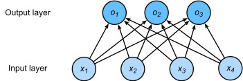
3.4. Softmax 회귀(regression) — Dive into Deep Learning documentation
ko.d2l.ai
Linear Regression 이 아닌 Softmax Regression에 대한 개념 설명을 하는 장
'Dive into Deep Learning > D2L Linear Neural Networks' 카테고리의 다른 글
| D2L - 4.3. The Base Classification Model (0) | 2023.06.26 |
|---|---|
| D2L - 4.2. The Image Classification Dataset (0) | 2023.06.26 |
| D2L 4.1. Softmax Regression (1) | 2023.06.26 |
| D2L - 4. Linear Neural Networks for Classification (0) | 2023.06.26 |
| D2L - Local Environment Setting (0) | 2023.06.26 |
| D2L - 3.5. Concise Implementation of Linear Regression, 이미지 분류 데이터 (Fashion-MNIST) (0) | 2023.06.22 |
| D2L - 3.3. Synthetic Regression Data (0) | 2023.06.22 |
| D2L 3.2. Object-Oriented Design for Implementation (0) | 2023.06.22 |
| D2L 3.2. 선형 회귀를 처음부터 구현하기 (0) | 2023.06.22 |
| D2L 3.1. Linear Regression (0) | 2023.06.20 |