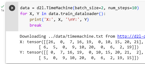
개발자로서 현장에서 일하면서 새로 접하는 기술들이나 알게된 정보 등을 정리하기 위한 블로그입니다. 운 좋게 미국에서 큰 회사들의 프로젝트에서 컬설턴트로 일하고 있어서 새로운 기술들을 접할 기회가 많이 있습니다. 미국의 IT 프로젝트에서 사용되는 툴들에 대해 많은 분들과 정보를 공유하고 싶습니다.
If you completed the exercises inSection 9.5, you would have seen that gradient clipping is vital to prevent the occasional massive gradients from destabilizing training. We hinted that the exploding gradients stem from backpropagating across long sequences. Before introducing a slew of modern RNN architectures, let’s take a closer look at howbackpropagationworks in sequence models in mathematical detail. Hopefully, this discussion will bring some precision to the notion ofvanishingandexplodinggradients. If you recall our discussion of forward and backward propagation through computational graphs when we introduced MLPs inSection 5.3, then forward propagation in RNNs should be relatively straightforward. Applying backpropagation in RNNs is calledbackpropagation through time(Werbos, 1990). This procedure requires us to expand (or unroll) the computational graph of an RNN one time step at a time. The unrolled RNN is essentially a feedforward neural network with the special property that the same parameters are repeated throughout the unrolled network, appearing at each time step. Then, just as in any feedforward neural network, we can apply the chain rule, backpropagating gradients through the unrolled net. The gradient with respect to each parameter must be summed across all places that the parameter occurs in the unrolled net. Handling such weight tying should be familiar from our chapters on convolutional neural networks.
섹션 9.5의 연습을 완료했다면 때때로 발생하는 대규모 기울기가 훈련을 불안정하게 만드는 것을 방지하기 위해 기울기 클리핑이 필수적이라는 것을 알았을 것입니다. 우리는 폭발하는 그래디언트가 긴 시퀀스에 걸쳐 역전파에서 비롯된다는 것을 암시했습니다. 수많은 최신 RNN 아키텍처를 소개하기 전에 시퀀스 모델에서 역전파가 수학적 세부 사항으로 작동하는 방식을 자세히 살펴보겠습니다. 바라건대, 이 논의가 그래디언트 소실 및 폭발의 개념에 어느 정도 정확성을 가져다 줄 것입니다. 섹션 5.3에서 MLP를 소개했을 때 계산 그래프를 통한 순방향 및 역방향 전파에 대한 논의를 기억한다면 RNN의 순방향 전파는 비교적 간단해야 합니다. RNN에서 역전파를 적용하는 것을 시간을 통한 역전파라고 합니다(Werbos, 1990). 이 절차에서는 한 번에 한 단계씩 RNN의 계산 그래프를 확장(또는 펼치기)해야 합니다. 언롤링된 RNN은 기본적으로 동일한 매개변수가 언롤링된 네트워크 전체에서 반복되어 각 시간 단계에 나타나는 특수 속성을 가진 피드포워드 신경망입니다. 그런 다음 피드포워드 신경망에서와 마찬가지로 체인 규칙을 적용하여 펼쳐진 그물을 통해 기울기를 역전파할 수 있습니다. 각 매개변수에 대한 기울기는 펼쳐진 그물에서 매개변수가 발생하는 모든 위치에서 합산되어야 합니다. 이러한 가중치 묶기를 처리하는 방법은 컨볼루션 신경망에 대한 장에서 익숙할 것입니다.
Complications arise because sequences can be rather long. It is not unusual to work with text sequences consisting of over a thousand tokens. Note that this poses problems both from a computational (too much memory) and optimization (numerical instability) standpoint. Input from the first step passes through over 1000 matrix products before arriving at the output, and another 1000 matrix products are required to compute the gradient. We now analyze what can go wrong and how to address it in practice.
시퀀스가 다소 길 수 있기 때문에 합병증이 발생합니다. 천 개가 넘는 토큰으로 구성된 텍스트 시퀀스로 작업하는 것은 드문 일이 아닙니다. 이는 계산(너무 많은 메모리) 및 최적화(수치적 불안정성) 관점에서 모두 문제를 제기합니다. 첫 번째 단계의 입력은 출력에 도달하기 전에 1000개 이상의 행렬 곱을 거치며 기울기를 계산하려면 또 다른 1000개의 행렬 곱이 필요합니다. 이제 무엇이 잘못될 수 있는지, 그리고 실제로 이를 해결하는 방법을 분석합니다.
9.7.1.Analysis of Gradients in RNNs
We start with a simplified model of how an RNN works. This model ignores details about the specifics of the hidden state and how it is updated. The mathematical notation here does not explicitly distinguish scalars, vectors, and matrices. We are just trying to develop some intuition. In this simplified model, we denoteℎtas the hidden state,xtas input, andotas output at time stept. Recall our discussions inSection 9.4.2that the input and the hidden state can be concatenated before being multiplied by one weight variable in the hidden layer. Thus, we usewℎandwoto indicate the weights of the hidden layer and the output layer, respectively. As a result, the hidden states and outputs at each time steps are
RNN 작동 방식에 대한 단순화된 모델부터 시작합니다. 이 모델은 숨겨진 상태의 세부 사항과 업데이트 방법에 대한 세부 정보를 무시합니다. 여기서 수학적 표기법은 스칼라, 벡터 및 행렬을 명시적으로 구분하지 않습니다. 우리는 직관을 개발하려고 노력하고 있습니다. 이 단순화된 모델에서 우리는 ℎt를 숨겨진 상태로, xt를 입력으로, ot를 시간 단계 t에서 출력으로 나타냅니다. 섹션 9.4.2에서 입력과 은닉 상태가 은닉층에서 하나의 가중치 변수에 의해 곱해지기 전에 연결될 수 있다는 논의를 상기하십시오. 따라서 wℎ와 wo를 사용하여 숨겨진 레이어와 출력 레이어의 가중치를 각각 나타냅니다. 결과적으로 각 시간 단계의 숨겨진 상태 및 출력은 다음과 같습니다.
wherefandgare transformations of the hidden layer and the output layer, respectively. Hence, we have a chain of values{…,(xt−1,ℎt−1,ot−1),(xt,ℎt,ot),…}that depend on each other via recurrent computation. The forward propagation is fairly straightforward. All we need is to loop through the(xt,ℎt,ot)triples one time step at a time. The discrepancy between output otand the desired targetytis then evaluated by an objective function across all theTtime steps as
여기서 f와 g는 각각 은닉층과 출력층의 변환입니다. 따라서 순환 계산을 통해 서로 의존하는 {...,(xt−1,ℎt−1,ot−1),(xt,ℎt,ot),...} 값 체인이 있습니다. 정방향 전파는 매우 간단합니다. 필요한 것은 한 번에 한 단계씩 (xt,ℎt,ot) 트리플을 반복하는 것입니다. 출력 ot와 원하는 목표 yt 사이의 불일치는 모든 T 시간 단계에서 목적 함수에 의해 다음과 같이 평가됩니다.
For backpropagation, matters are a bit trickier, especially when we compute the gradients with regard to the parameterswℎof the objective functionL. To be specific, by the chain rule,
역전파의 경우, 특히 목적 함수 L의 매개변수 wℎ에 대한 그래디언트를 계산할 때 문제가 좀 더 까다롭습니다. 구체적으로 체인 규칙에 따르면,
The first and the second factors of the product in(9.7.3)are easy to compute. The third factor∂ℎt/∂wℎis where things get tricky, since we need to recurrently compute the effect of the parameterwℎonℎt. According to the recurrent computation in(9.7.1),ℎtdepends on bothℎt−1andwℎ, where computation ofℎt−1also depends onwℎ. Thus, evaluating the total derivate ofℎtwith respect towℎusing the chain rule yields
(9.7.3)에서 제품의 첫 번째 및 두 번째 요소는 계산하기 쉽습니다. 세 번째 요소 ∂ℎt/∂wℎ는 ℎt에 대한 매개변수 wℎ의 효과를 반복적으로 계산해야 하기 때문에 상황이 까다로워집니다. (9.7.1)의 반복 계산에 따르면 ℎt는 ℎt-1과 wℎ 모두에 의존하며, 여기서 ℎt-1의 계산도 wℎ에 의존합니다. 따라서 체인 룰을 사용하여 wℎ에 대한 ℎt의 총 도함수를 평가하면 다음과 같습니다.
To derive the above gradient, assume that we have three sequences{at},{bt},{ct}satisfyinga0=0andat=bt+ctat−1fort=1,2,…. Then fort≥1, it is easy to show
위의 그래디언트를 도출하기 위해 t=1,2,…에 대해 a0=0 및 at=bt+ctat−1을 만족하는 세 개의 시퀀스 {at},{bt},{ct}가 있다고 가정합니다. 그런 다음 t≥1인 경우 표시하기 쉽습니다.
By substitutingat,bt, andctaccording to
다음에 따라 at, bt 및 ct를 대체하여
the gradient computation in(9.7.4)satisfiesat=bt+ctat−1. Thus, per(9.7.5), we can remove the recurrent computation in(9.7.4)with
(9.7.4)의 그래디언트 계산은 at=bt+ctat−1을 충족합니다. 따라서 (9.7.5)에 따라 (9.7.4)에서 반복 계산을 제거할 수 있습니다.
While we can use the chain rule to compute∂ℎt/∂wℎrecursively, this chain can get very long whenevertis large. Let’s discuss a number of strategies for dealing with this problem.
체인 규칙을 사용하여 ∂ℎt/∂wℎ를 재귀적으로 계산할 수 있지만 이 체인은 t가 클 때마다 매우 길어질 수 있습니다. 이 문제를 처리하기 위한 여러 가지 전략에 대해 논의해 봅시다.
9.7.1.1.Full Computation
One idea might be to compute the full sum in(9.7.7). However, this is very slow and gradients can blow up, since subtle changes in the initial conditions can potentially affect the outcome a lot. That is, we could see things similar to the butterfly effect, where minimal changes in the initial conditions lead to disproportionate changes in the outcome. This is generally undesirable. After all, we are looking for robust estimators that generalize well. Hence this strategy is almost never used in practice.
한 가지 아이디어는 (9.7.7)에서 전체 합계를 계산하는 것입니다. 그러나 초기 조건의 미묘한 변화가 잠재적으로 결과에 많은 영향을 미칠 수 있기 때문에 이것은 매우 느리고 기울기가 폭발할 수 있습니다. 즉, 초기 조건의 최소한의 변화가 결과에 불균형한 변화를 가져오는 나비 효과와 유사한 현상을 볼 수 있습니다. 이것은 일반적으로 바람직하지 않습니다. 결국, 우리는 잘 일반화되는 강력한 추정기를 찾고 있습니다. 따라서 이 전략은 실제로 거의 사용되지 않습니다.
9.7.1.2.Truncating Time Steps
Alternatively, we can truncate the sum in(9.7.7)afterτ steps. This is what we have been discussing so far. This leads to anapproximationof the true gradient, simply by terminating the sum at∂ℎt−τ/∂wℎ. In practice this works quite well. It is what is commonly referred to as truncated backpropgation through time(Jaeger, 2002). One of the consequences of this is that the model focuses primarily on short-term influence rather than long-term consequences. This is actuallydesirable, since it biases the estimate towards simpler and more stable models.
또는 τ 단계 후에 합계를 (9.7.7)에서 자를 수 있습니다. 이것이 우리가 지금까지 논의한 것입니다. 이것은 단순히 ∂ℎt−τ/∂wℎ에서 합계를 종료함으로써 실제 그래디언트의 근사치로 이어집니다. 실제로 이것은 꽤 잘 작동합니다. 이것은 일반적으로 시간에 따른 절단된 역전파(truncated backpropgation)라고 합니다(Jaeger, 2002). 이것의 결과 중 하나는 모델이 장기적인 결과보다는 주로 단기적인 영향에 초점을 맞추고 있다는 것입니다. 이것은 추정치를 더 간단하고 안정적인 모델로 편향시키기 때문에 실제로 바람직합니다.
9.7.1.3.Randomized Truncation
Last, we can replace∂ℎt/∂wℎby a random variable which is correct in expectation but truncates the sequence. This is achieved by using a sequence of ξtwith predefined0≤πt≤1, whereP(ξt=0)=1−πtandP(ξt=πt−1)=πt, thusE[ξt]=1. We use this to replace the gradient∂ℎt/∂wℎin(9.7.4)with
마지막으로, 우리는 ∂ℎt/∂wℎ를 예측에는 맞지만 시퀀스를 자르는 임의의 변수로 대체할 수 있습니다. 이것은 미리 정의된 0≤πt≤1을 갖는 ξt의 시퀀스를 사용하여 달성되며, 여기서 P(ξt=0)=1−πt 및 P(ξt=πt−1)=πt이므로 E[ξt]=1입니다. 이것을 사용하여 (9.7.4)의 기울기 ∂ℎt/∂wℎ를
It follows from the definition of ξtthatE[zt]=∂ℎt/∂wℎ. Wheneverξt=0the recurrent computation terminates at that time stept. This leads to a weighted sum of sequences of varying lengths, where long sequences are rare but appropriately overweighted. This idea was proposed byTallec and Ollivier (2017).
E[zt]=∂ℎt/∂wℎ는 ξt의 정의에 따른다. ξt=0일 때마다 순환 계산은 해당 시간 단계 t에서 종료됩니다. 이것은 긴 시퀀스가 드물지만 적절하게 과중한 다양한 길이의 시퀀스의 가중 합계로 이어집니다. 이 아이디어는 Tallec과 Ollivier(2017)가 제안했습니다.
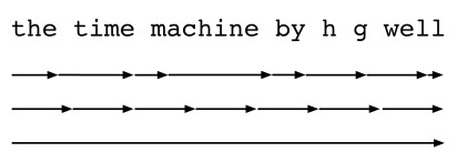
9.7.1.4.Comparing Strategies
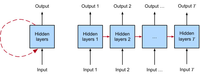
Fig. 9.7.1 Comparing strategies for computing gradients in RNNs. From top to bottom: randomized truncation, regular truncation, and full computation.
Fig. 9.7.1illustrates the three strategies when analyzing the first few characters ofThe Time Machineusing backpropagation through time for RNNs:
그림 9.7.1은 RNN에 대해 시간을 통한 역전파를 사용하여 The Time Machine의 처음 몇 문자를 분석할 때 세 가지 전략을 보여줍니다.
The first row is the randomized truncation that partitions the text into segments of varying lengths.
첫 번째 행은 텍스트를 다양한 길이의 세그먼트로 분할하는 임의 절단입니다.
The second row is the regular truncation that breaks the text into subsequences of the same length. This is what we have been doing in RNN experiments.
두 번째 행은 텍스트를 동일한 길이의 하위 시퀀스로 나누는 일반적인 잘림입니다. 이것이 우리가 RNN 실험에서 해온 것입니다.
The third row is the full backpropagation through time that leads to a computationally infeasible expression.
세 번째 행은 계산적으로 실현 불가능한 표현으로 이어지는 시간에 따른 전체 역전파입니다.
Unfortunately, while appealing in theory, randomized truncation does not work much better than regular truncation, most likely due to a number of factors. First, the effect of an observation after a number of backpropagation steps into the past is quite sufficient to capture dependencies in practice. Second, the increased variance counteracts the fact that the gradient is more accurate with more steps. Third, we actuallywantmodels that have only a short range of interactions. Hence, regularly truncated backpropagation through time has a slight regularizing effect that can be desirable.
불행하게도 이론적으로는 매력적이지만 임의 절단은 여러 가지 요인으로 인해 일반 절단보다 훨씬 더 잘 작동하지 않습니다. 첫째, 과거로의 여러 역전파 단계 후 관찰 효과는 실제로 종속성을 캡처하기에 충분합니다. 둘째, 증가된 분산은 그래디언트가 더 많은 단계로 더 정확하다는 사실을 상쇄합니다. 셋째, 우리는 실제로 짧은 범위의 상호 작용만 있는 모델을 원합니다. 따라서 시간에 따라 규칙적으로 절단된 역전파는 바람직할 수 있는 약간의 규칙화 효과를 갖습니다.
9.7.2.Backpropagation Through Time in Detail
After discussing the general principle, let’s discuss backpropagation through time in detail. Different from the analysis inSection 9.7.1, in the following we will show how to compute the gradients of the objective function with respect to all the decomposed model parameters. To keep things simple, we consider an RNN without bias parameters, whose activation function in the hidden layer uses the identity mapping (ϕ(x)=x). For time stept, let the single example input and the target bext∈ℝdandyt, respectively. The hidden stateℎt∈ℝℎand the outputot∈ℝqare computed as
일반적인 원칙을 논의한 후 시간에 따른 역전파에 대해 자세히 논의해 봅시다. 9.7.1절의 분석과 달리 다음에서는 분해된 모든 모델 매개변수에 대한 목적 함수의 기울기를 계산하는 방법을 보여줍니다. 단순함을 유지하기 위해 편향 매개변수가 없는 RNN을 고려합니다. 숨겨진 레이어의 활성화 함수는 ID 매핑(ϕ(x)=x)을 사용합니다. 시간 단계 t의 경우 단일 예제 입력과 대상을 각각 xt∈ℝd 및 yt로 둡니다. 숨겨진 상태 ℎt∈ℝℎ와 출력 ot∈ℝq는 다음과 같이 계산됩니다.
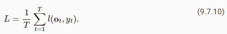
whereWℎx∈ℝℎ×d,Wℎℎ∈ℝℎ×ℎ, andWqℎ∈ℝq×ℎare the weight parameters. Denote byl(ot,yt)the loss at time stept. Our objective function, the loss overTtime steps from the beginning of the sequence is thus
여기서 Wℎx∈ℝℎ×d, Wℎℎ∈ℝℎ×ℎ 및 Wqℎ∈ℝq×ℎ는 가중치 매개변수입니다. l(ot,yt)는 시간 단계 t에서의 손실을 나타냅니다. 우리의 목적 함수, 시퀀스 시작부터 T 시간 단계에 걸친 손실은 다음과 같습니다.
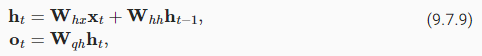
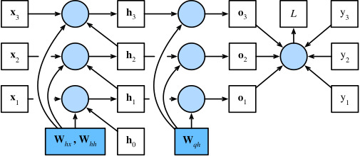
In order to visualize the dependencies among model variables and parameters during computation of the RNN, we can draw a computational graph for the model, as shown inFig. 9.7.2. For example, the computation of the hidden states of time step 3,ℎ3, depends on the model parametersWℎxandWℎℎ, the hidden state of the last time stepℎ2, and the input of the current time stepx3.
RNN을 계산하는 동안 모델 변수와 매개변수 간의 종속성을 시각화하기 위해 그림 9.7.2와 같이 모델에 대한 계산 그래프를 그릴 수 있습니다. 예를 들어, 시간 단계 3, ℎ3의 숨겨진 상태 계산은 모델 매개변수 Wℎx 및 Wℎℎ, 마지막 시간 단계 ℎ2의 숨겨진 상태 및 현재 시간 단계 x3의 입력에 따라 달라집니다.
Fig. 9.7.2 Computational graph showing dependencies for an RNN model with three time steps. Boxes represent variables (not shaded) or parameters (shaded) and circles represent operators.
As just mentioned, the model parameters inFig. 9.7.2areWℎx,Wℎℎ, andWqℎ. Generally, training this model requires gradient computation with respect to these parameters∂L/∂Wℎx,∂L/∂Wℎℎ, and∂L/∂Wqℎ. According to the dependencies inFig. 9.7.2, we can traverse in the opposite direction of the arrows to calculate and store the gradients in turn. To flexibly express the multiplication of matrices, vectors, and scalars of different shapes in the chain rule, we continue to use theprodoperator as described inSection 5.3.
방금 언급했듯이 그림 9.7.2의 모델 매개변수는 Wℎx, Wℎℎ 및 Wqℎ입니다. 일반적으로 이 모델을 훈련하려면 이러한 매개변수 ∂L/∂Wℎx, ∂L/∂Wℎℎ 및 ∂L/∂Wqℎ에 대한 그래디언트 계산이 필요합니다. 그림 9.7.2의 종속성에 따라 화살표의 반대 방향으로 순회하여 그래디언트를 차례로 계산하고 저장할 수 있습니다. 행렬, 벡터, 서로 다른 모양의 스칼라의 곱셈을 체인 룰에서 유연하게 표현하기 위해 섹션 5.3에서 설명한 대로 prod 연산자를 계속 사용합니다.
First of all, differentiating the objective function with respect to the model output at any time steptis fairly straightforward:
우선, 임의의 시간 단계 t에서 모델 출력과 관련하여 목적 함수를 미분하는 것은 매우 간단합니다.
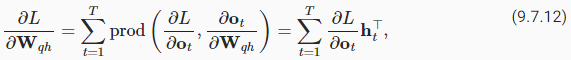
Now, we can calculate the gradient of the objective with respect to the parameterWqℎin the output layer:∂L/∂Wqℎ∈ℝq×ℎ. Based onFig. 9.7.2, the objectiveLdepends onWqℎviao1,…,oT. Using the chain rule yields where∂L//∂otis given by(9.7.11).
이제 출력 레이어의 매개변수 Wqℎ에 대한 목표 기울기를 계산할 수 있습니다: ∂L/∂Wqℎ∈ℝq×ℎ. 그림 9.7.2에 따라 목표 L은 o1,…,oT를 통해 Wqℎ에 따라 달라집니다. 체인 규칙을 사용하면 ∂L//∂ot가 (9.7.11)에 의해 제공됩니다.
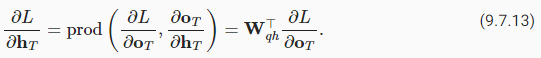
Next, as shown inFig. 9.7.2, at the final time stepT, the objective functionLdepends on the hidden stateℎTonly viaoT. Therefore, we can easily find the gradient ∂L/∂ℎt∈ℝℎusing the chain rule:
다음으로 그림 9.7.2에서와 같이 최종 시간 단계 T에서 목적 함수 L은 oT를 통해서만 숨겨진 상태 ℎT에 의존합니다. 따라서 체인 규칙을 사용하여 기울기 ∂L/∂ℎt∈ℝℎ를 쉽게 찾을 수 있습니다.
It gets trickier for any time stept<T, where the objective functionLdepends onℎtviaℎt+1andot. According to the chain rule, the gradient of the hidden state∂L/∂ℎt∈ℝℎat any time stept<Tcan be recurrently computed as:
목적 함수 L이 ℎt+1 및 ot를 통해 ℎt에 의존하는 임의의 시간 단계 t<T에 대해 더 까다로워집니다. 체인 규칙에 따라 임의의 시간 단계 t<T에서 숨겨진 상태 ∂L/ ∂ℎt∈ℝℎ의 기울기는 다음과 같이 반복적으로 계산할 수 있습니다.
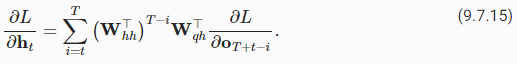
For analysis, expanding the recurrent computation for any time step1≤t≤Tgives
분석을 위해 임의의 시간 단계 1≤t≤T에 대한 반복 계산을 확장하면 다음이 제공됩니다.
We can see from(9.7.15)that this simple linear example already exhibits some key problems of long sequence models: it involves potentially very large powers ofWℎℎ⊤. In it, eigenvalues smaller than 1 vanish and eigenvalues larger than 1 diverge. This is numerically unstable, which manifests itself in the form of vanishing and exploding gradients. One way to address this is to truncate the time steps at a computationally convenient size as discussed inSection 9.7.1. In practice, this truncation can also be effected by detaching the gradient after a given number of time steps. Later on, we will see how more sophisticated sequence models such as long short-term memory can alleviate this further.
우리는 (9.7.15)에서 이 간단한 선형 예제가 이미 긴 시퀀스 모델의 몇 가지 주요 문제를 보여주고 있음을 알 수 있습니다. 잠재적으로 매우 큰 Wℎℎ⊤의 거듭제곱이 관련됩니다. 그 안에서 1보다 작은 고유값은 사라지고 1보다 큰 고유값은 발산한다. 이것은 수치적으로 불안정하며 기울기가 사라지고 폭발하는 형태로 나타납니다. 이 문제를 해결하는 한 가지 방법은 섹션 9.7.1에서 설명한 것처럼 계산상 편리한 크기로 시간 단계를 자르는 것입니다. 실제로 이 잘림은 주어진 시간 단계 수 후에 기울기를 분리하여 영향을 줄 수도 있습니다. 나중에 우리는 장단기 기억과 같은 더 정교한 시퀀스 모델이 이것을 어떻게 더 완화할 수 있는지 보게 될 것입니다.
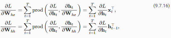
Finally,Fig. 9.7.2shows that the objective functionLdepends on model parametersWℎxandWℎℎin the hidden layer via hidden statesℎ1,…,ℎT. To compute gradients with respect to such parameters ∂L/∂Wℎx∈ℝℎ×dandL/∂Wℎℎ∈ℝℎ×ℎ, we apply the chain rule that gives
마지막으로 그림 9.7.2는 목적 함수 L이 숨겨진 상태 ℎ1,… 이러한 매개변수 ∂L/∂Wℎx∈ℝℎ×d 및 L/∂Wℎℎ∈ℝℎ×ℎ와 관련하여 기울기를 계산하기 위해 다음과 같은 체인 규칙을 적용합니다.
where∂L/∂ℎtthat is recurrently computed by(9.7.13)and(9.7.14)is the key quantity that affects the numerical stability.
여기서 (9.7.13)과 (9.7.14)에 의해 반복적으로 계산되는 ∂L/∂ℎt는 수치 안정성에 영향을 미치는 핵심 수량입니다.
Since backpropagation through time is the application of backpropagation in RNNs, as we have explained inSection 5.3, training RNNs alternates forward propagation with backpropagation through time. Besides, backpropagation through time computes and stores the above gradients in turn. Specifically, stored intermediate values are reused to avoid duplicate calculations, such as storing∂L/∂ℎtto be used in computation of both∂L/∂Wℎxand∂L/∂Wℎℎ.
시간을 통한 역전파는 RNN에서 역전파를 적용한 것이므로 섹션 5.3에서 설명한 것처럼 훈련 RNN은 순방향 전파와 시간을 통한 역전파를 번갈아 사용합니다. 게다가, 시간을 통한 역전파는 위의 그래디언트를 차례로 계산하고 저장합니다. 구체적으로, ∂L/∂Wℎx 및 ∂L/∂Wℎℎ의 계산에 사용되는 ∂L/∂ℎt를 저장하는 것과 같이, 저장된 중간 값은 중복 계산을 피하기 위해 재사용됩니다.
9.7.3.Summary
Backpropagation through time is merely an application of backpropagation to sequence models with a hidden state. Truncation is needed for computational convenience and numerical stability, such as regular truncation and randomized truncation. High powers of matrices can lead to divergent or vanishing eigenvalues. This manifests itself in the form of exploding or vanishing gradients. For efficient computation, intermediate values are cached during backpropagation through time.
시간에 따른 역전파는 은닉 상태의 시퀀스 모델에 역전파를 적용한 것일 뿐입니다. Truncation은 regular truncation, randomized truncation과 같이 계산의 편리성과 수치적 안정성을 위해 필요합니다. 행렬의 거듭제곱이 높으면 고유값이 발산하거나 사라질 수 있습니다. 이는 그라데이션이 폭발하거나 사라지는 형태로 나타납니다. 효율적인 계산을 위해 시간을 통해 역전파하는 동안 중간 값이 캐시됩니다.
9.6.Concise Implementation of Recurrent Neural Networks
Like most of our from-scratch implementations,Section 9.5was designed to provide insight into how each component works. But when you’re using RNNs every day or writing production code, you will want to rely more on libraries that cut down on both implementation time (by supplying library code for common models and functions) and computation time (by optimizing the heck out of these library implementations). This section will show you how to implement the same language model more efficiently using the high-level API provided by your deep learning framework. We begin, as before, by loadingThe Time Machinedataset.
대부분의 초기 구현과 마찬가지로 섹션 9.5는 각 구성 요소의 작동 방식에 대한 통찰력을 제공하도록 설계되었습니다. 그러나 매일 RNN을 사용하거나 프로덕션 코드를 작성할 때 구현 시간(공통 모델 및 함수에 대한 라이브러리 코드 제공)과 계산 시간(최적화를 통해)을 모두 줄이는 라이브러리에 더 의존하고 싶을 것입니다. 이러한 라이브러리 구현). 이 섹션에서는 딥 러닝 프레임워크에서 제공하는 고급 API를 사용하여 동일한 언어 모델을 보다 효율적으로 구현하는 방법을 보여줍니다. 이전과 마찬가지로 Time Machine 데이터 세트를 로드하여 시작합니다.
import torch
from torch import nn
from torch.nn import functional as F
from d2l import torch as d2l
9.6.1.Defining the Model
We define the following class using the RNN implemented by high-level APIs.
상위 수준 API에 의해 구현된 RNN을 사용하여 다음 클래스를 정의합니다.
class RNN(d2l.Module):  #@save
    """The RNN model implemented with high-level APIs."""
    def __init__(self, num_inputs, num_hiddens):
        super().__init__()
        self.save_hyperparameters()
        self.rnn = nn.RNN(num_inputs, num_hiddens)

    def forward(self, inputs, H=None):
        return self.rnn(inputs, H)
위 코드는 고수준 API를 사용하여 구현된 RNN(순환 신경망) 모델을 나타냅니다.
num_inputs: 입력 특성의 개수입니다.
num_hiddens: 은닉 상태의 차원 수입니다.
이 클래스의 __init__ 메서드는 다음과 같이 작동합니다:
num_inputs와 num_hiddens를 저장하고 부모 클래스인 d2l.Module의 생성자를 호출합니다.
nn.RNN을 사용하여 RNN 레이어를 생성합니다. 이 RNN 레이어는 입력의 크기가 num_inputs이고, 은닉 상태의 크기가 num_hiddens인 순환 신경망 레이어입니다.
forward 메서드는 다음과 같이 작동합니다:
inputs: 입력 데이터입니다. 시계열 데이터의 시간 스텝에 따른 특성들로 이루어진 3D 텐서입니다.
H: 초기 은닉 상태입니다. 기본값은 None이며, 필요한 경우 입력될 수 있습니다.
self.rnn을 통해 입력 데이터와 초기 은닉 상태를 RNN 레이어에 전달하여 순방향 계산을 수행합니다. 이 결과는 순방향 계산의 출력과 마지막 시간 스텝에서의 은닉 상태로 구성된 튜플로 반환됩니다.
이 코드는 고수준 API를 사용하여 간단한 RNN 모델을 구현하고 있습니다. RNN 모델은 순차 데이터를 처리하고 은닉 상태를 업데이트하는 데 사용될 수 있습니다.
torch.nn.RNN 클래스는 PyTorch에서 제공하는 순환 신경망(RNN) 레이어를 나타내는 클래스입니다. RNN은 시퀀스 데이터를 처리하는데 사용되며, 이전 단계의 출력이 다음 단계의 입력으로 사용되는 재귀 구조를 가집니다.
torch.nn.RNN 클래스는 다양한 매개변수를 통해 RNN 레이어의 동작을 구성할 수 있습니다. 주요 매개변수와 해당 역할은 다음과 같습니다:
input_size: 입력 특성의 크기입니다.
hidden_size: 은닉 상태의 크기입니다. RNN 레이어의 출력 및 은닉 상태의 크기가 됩니다.
num_layers: RNN의 층 수입니다. 디폴트 값은 1이며, 여러 층으로 쌓아 복잡한 모델을 만들 수 있습니다.
nonlinearity: 활성화 함수를 지정합니다. 디폴트는 'tanh'이며, 다른 옵션으로는 'relu' 등이 있습니다.
bias: 편향(bias)을 사용할지 여부를 결정합니다.
batch_first: True로 설정하면 입력 데이터의 shape를 (batch_size, seq_length, input_size)로 사용합니다.
dropout: 드롭아웃을 적용할 비율입니다.
bidirectional: 양방향 RNN을 사용할지 여부를 결정합니다.
이러한 매개변수를 설정하여 torch.nn.RNN 클래스로 RNN 레이어를 생성할 수 있으며, 이후 입력 데이터를 이 레이어에 전달하여 시퀀스 데이터의 처리를 수행할 수 있습니다.
Inheriting from theRNNLMScratchclass inSection 9.5, the followingRNNLMclass defines a complete RNN-based language model. Note that we need to create a separate fully connected output layer.
섹션 9.5의 RNNLMcratch 클래스에서 상속받은 다음 RNNLM 클래스는 완전한 RNN 기반 언어 모델을 정의합니다. 별도의 완전히 연결된 출력 계층을 만들어야 합니다.
class RNNLM(d2l.RNNLMScratch):  #@save
    """The RNN-based language model implemented with high-level APIs."""
    def init_params(self):
        self.linear = nn.LazyLinear(self.vocab_size)

    def output_layer(self, hiddens):
        return self.linear(hiddens).swapaxes(0, 1)
위 코드는 고수준 API를 사용하여 구현된 RNN 기반의 언어 모델인 RNNLM 클래스를 정의하고 있습니다.
이 클래스는 d2l.RNNLMScratch 클래스를 상속받습니다. RNNLMScratch 클래스는 이전 대화에서 고수준 API를 사용하여 구현된 RNN 언어 모델의 기본 구현을 포함하고 있습니다.
RNNLM 클래스의 init_params 메서드는 다음과 같이 작동합니다:
nn.LazyLinear를 사용하여 선형 레이어를 생성합니다. 이 레이어의 출력 크기는 어휘 크기(vocab_size)로 설정됩니다.
output_layer 메서드는 다음과 같이 작동합니다:
hiddens: RNN의 은닉 상태입니다. 각 시간 스텝마다의 은닉 상태들로 구성된 텐서입니다.
self.linear 레이어를 통해 은닉 상태를 선형 변환하여 언어 모델의 출력을 생성합니다. 출력 텐서의 크기는 (num_steps, batch_size, vocab_size)로 되며, 시간 스텝을 따라 텐서의 차원이 바뀌도록 swapaxes(0, 1) 메서드를 사용하여 차원을 바꿔줍니다.
이를 통해 RNNLM 클래스는 고수준 API를 사용하여 RNNLMScratch 클래스의 구현을 더 간결하고 편리하게 나타내고 있습니다.
9.6.2.Training and Predicting
Before training the model, let’s make a prediction with a model initialized with random weights. Given that we have not trained the network, it will generate nonsensical predictions.
모델을 훈련시키기 전에 임의의 가중치로 초기화된 모델로 예측을 해봅시다. 우리가 네트워크를 훈련시키지 않았다면 무의미한 예측을 생성할 것입니다.
data = d2l.TimeMachine(batch_size=1024, num_steps=32)
rnn = RNN(num_inputs=len(data.vocab), num_hiddens=32)
model = RNNLM(rnn, vocab_size=len(data.vocab), lr=1)
model.predict('it has', 20, data.vocab)
위 코드는 고수준 API를 사용하여 구현된 RNN 기반의 언어 모델인 RNNLM 클래스를 활용하여 예측하는 과정을 보여줍니다.
d2l.TimeMachine 클래스를 사용하여 데이터를 로드합니다. 이 데이터는 언어 모델 학습에 사용되는 텍스트 데이터입니다.
RNN 클래스를 인스턴스화하여 RNN 모델을 생성합니다. 이 클래스는 고수준 API를 사용하여 RNN 레이어를 포함하고 있습니다.
RNNLM 클래스를 인스턴스화하여 언어 모델을 생성합니다. 이 클래스는 RNN 클래스를 기반으로 하며, 모델의 출력 레이어로 nn.LazyLinear 레이어를 사용하여 언어 모델의 예측을 수행합니다.
model.predict 메서드를 사용하여 주어진 입력 문자열('it has')에 대한 모델의 예측을 생성합니다. 이 메서드는 주어진 입력 문자열 다음에 오는 문자들을 모델을 사용하여 예측합니다. 마지막 인자로는 어휘 사전(data.vocab)을 전달하여 예측된 정수값을 문자로 변환합니다.
이를 통해 고수준 API를 사용하여 구현된 RNN 언어 모델을 활용하여 주어진 입력에 대한 다음 문자 예측을 수행하는 과정을 보여줍니다.
'it hasgggggggggggggggggggg'
Next, we train our model, leveraging the high-level API.
d2l.Trainer 클래스를 인스턴스화하여 트레이너를 생성합니다. 이 클래스는 모델 학습에 관련된 설정을 지정할 수 있는 기능을 제공합니다. 여기서 max_epochs는 최대 에포크 수를, gradient_clip_val은 그래디언트 클리핑을 수행할 임계값을, num_gpus는 사용할 GPU 수를 나타냅니다.
trainer.fit 메서드를 사용하여 모델을 학습합니다. 첫 번째 인자로는 학습할 모델(model)을, 두 번째 인자로는 학습 데이터(data)를 전달합니다. 이 메서드는 지정한 최대 에포크 수(max_epochs) 동안 모델을 학습시킵니다. 학습 중에는 그래디언트 클리핑이 적용될 수 있습니다(gradient_clip_val에 지정한 임계값을 넘어서지 않도록 그래디언트를 조정).
이를 통해 d2l.Trainer를 사용하여 모델을 학습하는 방법을 보여줍니다.
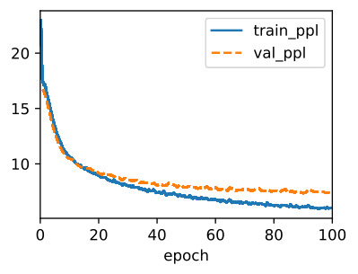
Compared withSection 9.5, this model achieves comparable perplexity, but runs faster due to the optimized implementations. As before, we can generate predicted tokens following the specified prefix string.
섹션 9.5와 비교하여 이 모델은 비슷한 복잡성을 달성하지만 최적화된 구현으로 인해 더 빠르게 실행됩니다. 이전과 마찬가지로 지정된 접두사 문자열 다음에 예측 토큰을 생성할 수 있습니다.
model.predict 메서드를 호출하여 텍스트를 생성합니다. 이 메서드는 생성하려는 텍스트의 시작 점인 prefix, 생성할 텍스트의 길이인 num_preds, 사용할 어휘 사전인 vocab, 그리고 어떤 디바이스(GPU 또는 CPU)에서 연산을 수행할지를 나타내는 device를 인자로 받습니다.
이 메서드는 outputs라는 리스트를 생성하고, 먼저 prefix의 첫 번째 단어를 outputs에 추가합니다. 그런 다음 생성된 텍스트의 길이인 num_preds만큼 반복문을 수행합니다.
각 반복에서 현재까지 생성된 텍스트를 바탕으로 다음 단어를 생성하고 outputs에 추가합니다. 이를 위해 현재 단어에 해당하는 인덱스를 X로 변환하고, 모델에 입력으로 넣어서 다음 단어를 예측합니다.
이렇게 생성된 텍스트의 인덱스를 outputs에 추가합니다.
모든 반복이 끝나면 outputs 리스트에 저장된 인덱스들을 어휘 사전을 이용해 실제 단어로 변환하여 결합하여 생성된 텍스트를 반환합니다.
즉, model.predict 메서드는 주어진 접두어(prefix)와 모델을 사용하여 주어진 길이(num_preds)만큼의 텍스트를 생성하는 기능을 수행합니다.
'it has and the time trave '
9.6.3.Summary
High-level APIs in deep learning frameworks provide implementations of standard RNNs. These libraries help you to avoid wasting time reimplementing standard models. Moreover, framework implementations are often highly optimized, leading to significant (computational) performance gains as compared to implementations from scratch.
딥 러닝 프레임워크의 고급 API는 표준 RNN 구현을 제공합니다. 이러한 라이브러리는 표준 모델을 다시 구현하는 데 시간을 낭비하지 않도록 도와줍니다. 또한 프레임워크 구현은 종종 고도로 최적화되어 처음부터 구현하는 것과 비교할 때 상당한 (계산) 성능 향상을 가져옵니다.
RNN High-Level API에 대해서...
In the context of deep learning frameworks like PyTorch, a high-level API for Recurrent Neural Networks (RNNs) refers to a set of pre-built and easy-to-use functions, classes, and modules that abstract away the low-level details of creating and training RNN models. This high-level API simplifies the process of working with RNNs by providing ready-to-use components, reducing the need for manual implementation and allowing practitioners to focus more on designing and experimenting with models.
딥 러닝 프레임워크인 PyTorch에서의 고수준 API란 사전에 구축된 함수, 클래스, 모듈 세트를 의미합니다. 이러한 API는 재귀 신경망(RNN) 모델을 생성하고 훈련시키는 저수준 세부 사항을 추상화하여 제공합니다. 이 고수준 API는 RNN 작업을 간단하게 만들어주며, 수동으로 구현할 필요성을 줄여주어 모델 디자인 및 실험에 집중할 수 있도록 도와줍니다.
The high-level API for RNNs often includes the following features:
고수준 RNN API는 일반적으로 다음과 같은 기능을 포함합니다:
Pre-built RNN Layers: High-level APIs provide pre-built RNN layer classes with configurable parameters, such as the number of hidden units, number of layers, dropout rates, and more. These classes encapsulate the underlying complexity of RNN cell creation and management.
미리 구축된 RNN 레이어: 고수준 API는 설정 가능한 매개변수(숨겨진 유닛 수, 레이어 수, 드롭아웃 비율 등)를 가진 미리 구축된 RNN 레이어 클래스를 제공합니다. 이러한 클래스는 RNN 셀 생성 및 관리의 기본 복잡성을 캡슐화합니다.
Sequence Handling: They offer convenient functions for dealing with sequences, such as padding, packing, and unpacking sequences, making it easier to work with variable-length inputs.
시퀀스 처리: 시퀀스(열) 처리와 관련된 편리한 기능을 제공하여 패딩, 언패킹 등의 작업을 간편하게 처리할 수 있도록 합니다. 이는 가변 길이 입력과 작업하는 데 도움이 됩니다.
Bidirectional RNNs: Many high-level APIs support bidirectional RNNs out of the box, allowing the model to capture information from both past and future time steps.
양방향 RNN: 많은 고수준 API가 양방향 RNN을 지원하며, 이로 인해 모델이 과거 및 미래 시간 단계의 정보를 모두 캡처할 수 있습니다.
Batch First: They often allow you to specify whether the input data should have the batch dimension as the first dimension, simplifying the handling of batched data.
배치 우선: 입력 데이터의 배치 차원을 첫 번째 차원으로 설정할 수 있도록 허용하여 배치 데이터 처리를 간편하게 할 수 있도록 합니다.
Model Building: High-level APIs offer simple ways to construct complex models using RNN layers. They typically allow for stacking multiple layers, adding other types of layers, and creating custom architectures.
모델 구축: 고수준 API는 RNN 레이어를 사용하여 복잡한 모델을 간단하게 구성하는 방법을 제공합니다. 여러 레이어를 쌓거나 다른 유형의 레이어를 추가하고 사용자 정의 아키텍처를 만드는 것이 일반적입니다.
Training Loop: These APIs often provide training loops that abstract away the gradient calculation, optimization steps, and loss calculation, making the training process more streamlined.
훈련 루프: 이러한 API는 경사 계산, 최적화 단계 및 손실 계산 등의 세부 사항을 추상화하는 훈련 루프를 제공하여 훈련 과정을 더 간단하게 만들어줍니다.
Model Saving and Loading: High-level APIs provide methods for saving and loading trained models, which is crucial for model deployment and further experimentation.
모델 저장 및 불러오기: 고수준 API는 훈련된 모델을 저장하고 불러오는 방법을 제공하여 모델 배포 및 추가 실험에 필요한 기능을 제공합니다.
Examples of high-level APIs for RNNs in PyTorch include nn.RNN, nn.LSTM, and nn.GRU modules. These modules encapsulate the functionality of RNN cells and provide a simpler interface for building and training RNN-based models.
PyTorch에서의 고수준 RNN API 예시로는 nn.RNN, nn.LSTM, nn.GRU 모듈이 있습니다. 이러한 모듈은 RNN 셀의 기능을 캡슐화하고 구축 및 훈련하기 위한 더 간단한 인터페이스를 제공합니다.
9.6.4.Exercises
Can you make the RNN model overfit using the high-level APIs?
Implement the autoregressive model ofSection 9.1using an RNN.
9.5.Recurrent Neural Network Implementation from Scratch
We are now ready to implement an RNN from scratch. In particular, we will train this RNN to function as a character-level language model (seeSection 9.4) and train it on a corpus consisting of the entire text of H. G. Wells’The Time Machine, following the data processing steps outlined inSection 9.2. We start by loading the dataset.
이제 처음부터 RNN을 구현할 준비가 되었습니다. 특히, 우리는 이 RNN이 문자 수준 언어 모델(섹션 9.4 참조)로 기능하도록 훈련하고 H. G. Wells의 The Time Machine의 전체 텍스트로 구성된 코퍼스에서 섹션 9.2에 설명된 데이터 처리 단계에 따라 훈련할 것입니다. . 데이터 세트를 로드하는 것으로 시작합니다.
%matplotlib inline
import math
import torch
from torch import nn
from torch.nn import functional as F
from d2l import torch as d2l
9.5.1.RNN Model
We begin by defining a class to implement the RNN model (Section 9.4.2). Note that the number of hidden unitsnum_hiddensis a tunable hyperparameter.
RNN 모델을 구현하기 위한 클래스를 정의하는 것으로 시작합니다(섹션 9.4.2). 은닉 유닛의 수 num_hiddens는 조정 가능한 하이퍼파라미터입니다.
위 코드는 PyTorch를 사용하여 구현된 간단한 RNN 모델을 나타냅니다. 이 코드는 스크래치에서 RNN을 구축하는 방법을 보여줍니다.
RNNScratch 클래스는 d2l.Module 클래스를 상속하여 정의되었습니다. 이 클래스는 RNN 모델의 구조와 가중치를 정의합니다.
__init__ 메서드: RNN 모델의 초기화를 담당합니다. 모델의 하이퍼파라미터(num_inputs, num_hiddens, sigma)를 저장하고, 입력과 숨겨진 상태 사이의 가중치 행렬 W_xh와 숨겨진 상태 간의 가중치 행렬 W_hh, 그리고 숨겨진 상태의 편향 b_h를 정의합니다. 이때 가중치 행렬과 편향은 무작위로 초기화되며, 초기화 값에는 sigma를 곱하여 스케일링합니다.
이렇게 정의된 RNNScratch 클래스는 스크래치에서 구현된 간단한 RNN 모델을 나타내며, 이 모델은 입력과 이전 숨겨진 상태를 활용하여 새로운 숨겨진 상태를 계산하는 역할을 합니다.
Theforwardmethod below defines how to compute the output and hidden state at any time step, given the current input and the state of the model at the previous time step. Note that the RNN model loops through the outermost dimension ofinputs, updating the hidden state one time step at a time. The model here uses atanhactivation function (Section 5.1.2.3).
아래의 전달 방법은 현재 입력과 이전 시간 단계에서 모델의 상태가 주어지면 임의의 시간 단계에서 출력 및 숨겨진 상태를 계산하는 방법을 정의합니다. RNN 모델은 한 번에 한 단계씩 숨겨진 상태를 업데이트하면서 입력의 가장 바깥쪽 차원을 반복합니다. 여기서 모델은 tanh 활성화 기능을 사용합니다(섹션 5.1.2.3).
@d2l.add_to_class(RNNScratch) #@save
def forward(self, inputs, state=None):
if state is None:
# Initial state with shape: (batch_size, num_hiddens)
state = torch.zeros((inputs.shape[1], self.num_hiddens),
device=inputs.device)
else:
state, = state
outputs = []
for X in inputs: # Shape of inputs: (num_steps, batch_size, num_inputs)
state = torch.tanh(torch.matmul(X, self.W_xh) +
torch.matmul(state, self.W_hh) + self.b_h)
outputs.append(state)
return outputs, state
위 코드는 앞서 정의한 RNNScratch 클래스에 forward 메서드를 추가하는 부분입니다. 이 메서드는 RNN 모델의 순전파(forward pass) 연산을 정의합니다.
forward 메서드: RNN 모델의 순전파 연산을 정의합니다. 이 메서드는 두 개의 입력을 받습니다. 첫 번째 입력 inputs는 시계열 데이터의 배치를 나타내는 텐서입니다. 두 번째 입력 state는 초기 숨겨진 상태로, 기본값은 None으로 지정되어 있습니다. 이 메서드는 RNN 모델이 입력 데이터를 처리하면서 각 시간 단계에서 숨겨진 상태를 계산합니다.
if state is None:: 초기 숨겨진 상태가 None인 경우에는 모든 배치에 대해 초기 숨겨진 상태를 0으로 설정합니다.
else:: 초기 숨겨진 상태가 None이 아닌 경우에는 입력으로 들어온 state 값을 사용합니다.
outputs = []: 각 시간 단계에서의 숨겨진 상태를 저장할 리스트를 초기화합니다.
for X in inputs:: 입력 데이터 inputs는 시간 단계별로 반복되는데, 이를 각 시간 단계에서 처리합니다. X는 현재 시간 단계의 입력 데이터를 나타냅니다.
state = torch.tanh(...): RNN의 숨겨진 상태 갱신을 위한 연산을 수행합니다. 입력 X와 이전 숨겨진 상태를 활용하여 새로운 숨겨진 상태를 계산합니다. 이때 활성화 함수로 tanh를 사용합니다.
outputs.append(state): 계산된 숨겨진 상태를 outputs 리스트에 추가합니다.
return outputs, state: 모든 시간 단계에 대한 숨겨진 상태 리스트 outputs와 마지막 숨겨진 상태 state를 반환합니다.
이렇게 정의된 forward 메서드는 RNN 모델의 순전파 연산을 구현한 것으로, 입력 데이터에 대한 순차적인 처리를 통해 시계열 데이터의 패턴을 학습합니다.
We can feed a minibatch of input sequences into an RNN model as follows.
위 코드는 RNNScratch 클래스를 사용하여 RNN 모델을 생성하고, 입력 데이터에 대한 순전파 연산을 수행하는 예제입니다.
batch_size, num_inputs, num_hiddens, num_steps: 각각 배치 크기, 입력 특성의 개수, 숨겨진 상태의 크기, 시간 단계 수를 지정합니다.
rnn = RNNScratch(num_inputs, num_hiddens): 위에서 정의한 RNNScratch 클래스를 생성합니다. 이 때 입력 특성의 개수 num_inputs와 숨겨진 상태의 크기 num_hiddens를 지정하여 모델을 초기화합니다.
X = torch.ones((num_steps, batch_size, num_inputs)): 시계열 데이터에 해당하는 입력 X를 생성합니다. 입력 데이터의 크기는 (num_steps, batch_size, num_inputs)입니다. 이때 각 시간 단계의 입력은 모두 1로 초기화되었습니다.
outputs, state = rnn(X): 생성한 RNN 모델을 사용하여 입력 데이터 X에 대한 순전파 연산을 수행합니다. 이를 통해 각 시간 단계에서의 숨겨진 상태 리스트 outputs와 마지막 숨겨진 상태 state가 반환됩니다.
즉, 위 코드는 시계열 데이터에 대한 입력 X를 사용하여 RNN 모델을 통해 각 시간 단계에서의 숨겨진 상태를 계산하는 예제입니다.
Let’s check whether the RNN model produces results of the correct shapes to ensure that the dimensionality of the hidden state remains unchanged.
숨겨진 상태의 차원이 변경되지 않도록 RNN 모델이 올바른 모양의 결과를 생성하는지 확인합시다.
def check_len(a, n): #@save
"""Check the length of a list."""
assert len(a) == n, f'list\'s length {len(a)} != expected length {n}'
def check_shape(a, shape): #@save
"""Check the shape of a tensor."""
assert a.shape == shape, \
f'tensor\'s shape {a.shape} != expected shape {shape}'
check_len(outputs, num_steps)
check_shape(outputs[0], (batch_size, num_hiddens))
check_shape(state, (batch_size, num_hiddens))
위 코드는 길이와 텐서의 형태를 확인하는 두 개의 함수 check_len과 check_shape를 정의하고, 이를 활용하여 연산 결과의 길이와 형태를 검증하는 예제입니다.
check_len(a, n): 리스트 a의 길이가 n과 일치하는지 확인하는 함수입니다. 만약 길이가 일치하지 않는다면 AssertionError를 발생시킵니다.
check_shape(a, shape): 텐서 a의 형태(shape)가 주어진 shape와 일치하는지 확인하는 함수입니다. 만약 형태가 일치하지 않는다면 AssertionError를 발생시킵니다.
그리고 마지막 부분에서는 위에서 계산한 outputs와 state의 길이 및 형태를 확인하는 작업을 수행합니다. 예를 들어 outputs는 RNN 모델의 출력이고, state는 마지막 숨겨진 상태입니다. num_steps는 시간 단계 수, batch_size는 배치 크기, num_hiddens는 숨겨진 상태의 크기입니다. 이 코드는 계산 결과의 정확성을 검증하기 위해 사용됩니다.
따라서 이 코드는 각 시간 단계에서의 숨겨진 상태 리스트와 마지막 숨겨진 상태의 형태와 길이를 검증하는 예제입니다.
9.5.2.RNN-based Language Model
The followingRNNLMScratchclass defines an RNN-based language model, where we pass in our RNN via thernnargument of the__init__method. When training language models, the inputs and outputs are from the same vocabulary. Hence, they have the same dimension, which is equal to the vocabulary size. Note that we use perplexity to evaluate the model. As discussed inSection 9.3.2, this ensures that sequences of different length are comparable.
다음 RNNLMScratch 클래스는 __init__ 메서드의 rnn 인수를 통해 RNN을 전달하는 RNN 기반 언어 모델을 정의합니다. 언어 모델을 훈련할 때 입력과 출력은 동일한 어휘에서 나옵니다. 따라서 그들은 어휘 크기와 동일한 차원을 가집니다. 우리는 perplexity를 사용하여 모델을 평가합니다. 섹션 9.3.2에서 논의된 바와 같이, 이것은 다른 길이의 시퀀스가 비교 가능하도록 보장합니다.
class RNNLMScratch(d2l.Classifier): #@save
"""The RNN-based language model implemented from scratch."""
def __init__(self, rnn, vocab_size, lr=0.01):
super().__init__()
self.save_hyperparameters()
self.init_params()
def init_params(self):
self.W_hq = nn.Parameter(
torch.randn(
self.rnn.num_hiddens, self.vocab_size) * self.rnn.sigma)
self.b_q = nn.Parameter(torch.zeros(self.vocab_size))
def training_step(self, batch):
l = self.loss(self(*batch[:-1]), batch[-1])
self.plot('ppl', torch.exp(l), train=True)
return l
def validation_step(self, batch):
l = self.loss(self(*batch[:-1]), batch[-1])
self.plot('ppl', torch.exp(l), train=False)
위 코드는 RNN 기반의 언어 모델인 RNNLMScratch 클래스를 정의하는 예제입니다.
RNNLMScratch 클래스는 d2l.Classifier 클래스를 상속받습니다. d2l은 Deep Learning for Coders 라이브러리로, 간단한 딥 러닝 모델을 쉽게 정의하고 학습하는 기능을 제공합니다.
__init__(self, rnn, vocab_size, lr=0.01): 생성자 메서드에서 모델을 초기화합니다. 인자로는 RNN 모델 (rnn), 어휘 크기 (vocab_size), 학습률 (lr)을 받습니다.
init_params(self): 파라미터를 초기화하는 메서드입니다. W_hq는 RNN의 숨겨진 상태와 어휘 크기에 대한 가중치 매트릭스이며, b_q는 편향입니다.
training_step(self, batch): 학습 단계를 수행하는 메서드입니다. 주어진 배치를 이용하여 모델의 예측과 실제 값 간의 손실을 계산하고, perplexity 값을 계산하여 시각화합니다.
validation_step(self, batch): 검증 단계를 수행하는 메서드로, 학습 단계와 비슷한 방식으로 손실과 perplexity 값을 계산하고 시각화합니다.
이 클래스는 RNN을 기반으로 한 언어 모델을 정의하고 학습과 검증 단계에서의 손실 값을 계산하여 모니터링하는 기능을 제공합니다.
9.5.2.1.One-Hot Encoding
Recall that each token is represented by a numerical index indicating the position in the vocabulary of the corresponding word/character/word-piece. You might be tempted to build a neural network with a single input node (at each time step), where the index could be fed in as a scalar value. This works when we are dealing with numerical inputs like price or temperature, where any two values sufficiently close together should be treated similarly. But this does not quite make sense. The45thand46thwords in our vocabulary happen to be “their” and “said”, whose meanings are not remotely similar.
각 토큰은 해당 단어/문자/단어 조각의 어휘에서 위치를 나타내는 숫자 색인으로 표시됩니다. 인덱스가 스칼라 값으로 공급될 수 있는 단일 입력 노드(각 시간 단계에서)가 있는 신경망을 구축하고 싶을 수 있습니다. 이는 가격이나 온도와 같은 숫자 입력을 처리할 때 작동하며, 여기서 충분히 가까운 두 값은 유사하게 처리되어야 합니다. 그러나 이것은 말이 되지 않습니다. 우리 어휘의 45번째와 46번째 단어는 우연히 "their"와 "said"인데, 그 의미는 거의 비슷하지 않습니다.
When dealing with such categorical data, the most common strategy is to represent each item by aone-hot encoding(recall fromSection 4.1.1). A one-hot encoding is a vector whose length is given by the size of the vocabularyN, where all entries are set to0, except for the entry corresponding to our token, which is set to1. For example, if the vocabulary had 5 elements, then the one-hot vectors corresponding to indices 0 and 2 would be the following.
이러한 범주형 데이터를 처리할 때 가장 일반적인 전략은 원-핫 인코딩으로 각 항목을 나타내는 것입니다(섹션 4.1.1 참조). 원-핫 인코딩은 1로 설정된 토큰에 해당하는 항목을 제외하고 모든 항목이 0으로 설정되는 어휘 N의 크기로 길이가 주어지는 벡터입니다. 요소가 5개이면 인덱스 0과 2에 해당하는 원-핫 벡터는 다음과 같습니다.
F.one_hot(torch.tensor([0, 2]), 5)
위 코드는 F.one_hot 함수를 사용하여 정수를 원-핫 벡터로 변환하는 예제입니다.
F.one_hot(indices, num_classes): 주어진 인덱스(indices)에 대한 원-핫 벡터를 생성합니다. num_classes는 클래스의 총 개수입니다.
여기서는 [0, 2] 라는 인덱스 배열에 대하여 num_classes가 5인 원-핫 벡터를 생성하고 있습니다. 결과는 다음과 같습니다:
tensor([[1, 0, 0, 0, 0],
[0, 0, 1, 0, 0]])
첫 번째 원-핫 벡터는 인덱스 0을 나타내며, 두 번째 원-핫 벡터는 인덱스 2를 나타냅니다.
One-Hot Encoding 이란?
"One-Hot Encoding"은 범주형 데이터를 다루는 데 사용되는 데이터 인코딩 기법 중 하나입니다. 이 기법은 범주형 변수를 이진 벡터로 변환하여 컴퓨터 알고리즘에서 처리할 수 있게 합니다.
예를 들어, 주어진 범주형 변수가 {빨강, 파랑, 녹색}과 같은 색상 카테고리를 가진다고 가정해보겠습니다. One-Hot Encoding을 사용하면 각 색상은 다음과 같이 표현될 수 있습니다:
빨강: [1, 0, 0]
파랑: [0, 1, 0]
녹색: [0, 0, 1]
즉, 각 카테고리에 대해 하나의 차원만 1이고 나머지 차원은 0으로 채워진 이진 벡터로 표현하는 것입니다. 이러한 표현은 해당 카테고리를 고유하게 식별하면서도 컴퓨터 알고리즘이 이해하기 쉬운 형태로 변환합니다.
One-Hot Encoding은 주로 분류 문제에서 사용되며, 범주형 변수를 수치 데이터로 변환하여 기계 학습 모델에 입력할 수 있게 합니다.
The minibatches that we sample at each iteration will take the shape (batch size, number of time steps). Once representing each input as a one-hot vector, we can think of each minibatch as a three-dimensional tensor, where the length along the third axis is given by the vocabulary size (len(vocab)). We often transpose the input so that we will obtain an output of shape (number of time steps, batch size, vocabulary size). This will allow us to more conveniently loop through the outermost dimension for updating hidden states of a minibatch, time step by time step (e.g., in the aboveforwardmethod).
각 반복에서 샘플링하는 미니 배치는 모양(배치 크기, 시간 단계 수)을 취합니다. 각 입력을 원-핫 벡터로 나타내면 각 미니배치를 3차원 텐서로 생각할 수 있습니다. 여기서 세 번째 축의 길이는 어휘 크기(len(vocab))로 지정됩니다. 우리는 종종 모양(시간 단계 수, 배치 크기, 어휘 크기)의 출력을 얻을 수 있도록 입력을 전치합니다. 이렇게 하면 미니배치의 숨겨진 상태를 시간 단계별로 업데이트하기 위해 가장 바깥쪽 차원을 통해 더 편리하게 루프를 돌 수 있습니다(예: 위의 전달 방법).
one_hot 메서드는 입력 데이터를 원-핫 벡터 형태로 변환하는 역할을 합니다. 입력 데이터 X는 정수로 이루어진 텐서이며, 각 정수는 단어의 인덱스를 나타냅니다.
F.one_hot(indices, num_classes): 주어진 인덱스(indices)에 대한 원-핫 벡터를 생성합니다. num_classes는 클래스의 총 개수입니다.
one_hot 메서드는 입력 데이터 X를 행렬 전치하여 정렬하고, 그에 대해 F.one_hot 함수를 적용한 결과를 반환합니다. 반환된 텐서의 크기는 (num_steps, batch_size, vocab_size)입니다. 이렇게 변환된 원-핫 벡터는 모델의 입력으로 사용됩니다.
9.5.2.2.Transforming RNN Outputs
The language model uses a fully connected output layer to transform RNN outputs into token predictions at each time step.
언어 모델은 완전히 연결된 출력 계층을 사용하여 각 단계에서 RNN 출력을 토큰 예측으로 변환합니다.
위 코드는 RNNLMScratch 클래스에 두 가지 메서드인 output_layer와 forward를 추가하는 예제입니다.
output_layer 메서드: 이 메서드는 RNN 모델의 출력을 받아서 각 시간 단계에서의 결과를 통해 최종 출력을 생성합니다. 각 시간 단계의 RNN 출력 rnn_outputs를 받아서 해당 출력을 가중치 행렬 W_hq와 절편 b_q로 선형 변환하여 최종 출력을 생성합니다. 이후 시간 단계의 출력을 리스트로 묶어 반환합니다.
forward 메서드: 이 메서드는 입력 시퀀스 X와 초기 상태 state를 받아서 RNNLM 모델의 순방향 전달(forward pass)을 수행합니다. 먼저 one_hot 메서드를 사용하여 입력 시퀀스 X를 원-핫 벡터 형태로 변환한 embs를 생성합니다. 이후 RNN 모델에 embs를 입력으로 전달하여 RNN 출력 rnn_outputs를 얻습니다. 마지막으로 이 rnn_outputs를 output_layer 메서드에 전달하여 최종 출력을 생성하고 반환합니다.
이렇게 구현된 output_layer와 forward 메서드는 RNN 기반의 언어 모델의 순방향 전달 과정을 정의하고 모델의 출력을 계산합니다.
Let’s check whether the forward computation produces outputs with the correct shape.
위 코드는 RNNLMScratch 클래스의 인스턴스를 생성하고, 해당 모델에 입력 데이터를 전달하여 출력 형태를 확인하는 예제입니다.
model = RNNLMScratch(rnn, num_inputs): 이 코드는 RNNLMScratch 클래스의 인스턴스를 생성합니다. rnn은 RNN 모델의 인스턴스이며, num_inputs는 어휘 크기입니다. 이를 기반으로 모델이 초기화됩니다.
outputs = model(torch.ones((batch_size, num_steps), dtype=torch.int64)): 이 코드는 생성한 model에 입력 데이터를 전달하여 출력을 얻습니다. 입력 데이터는 (batch_size, num_steps) 형태의 크기를 가진 텐서입니다. 이 입력 데이터를 모델에 전달하면 모델의 순방향 전달이 실행되어 출력 텐서 outputs를 반환합니다.
check_shape(outputs, (batch_size, num_steps, num_inputs)): 이 코드는 check_shape 함수를 사용하여 outputs의 형태가 (batch_size, num_steps, num_inputs)와 동일한지 확인합니다. 이를 통해 모델의 출력 형태를 검사합니다.
즉, 위 코드는 RNN 기반의 언어 모델인 RNNLMScratch의 인스턴스를 생성하고, 입력 데이터를 이 모델에 전달하여 출력의 형태를 검사하는 과정을 나타내는 예제입니다.
9.5.3.Gradient Clipping
While you are already used to thinking of neural networks as “deep” in the sense that many layers separate the input and output even within a single time step, the length of the sequence introduces a new notion of depth. In addition to the passing through the network in the input-to-output direction, inputs at the first time step must pass through a chain ofTlayers along the time steps in order to influence the output of the model at the final time step. Taking the backwards view, in each iteration, we backpropagate gradients through time, resulting in a chain of matrix-products with lengthO(T). As mentioned inSection 5.4, this can result in numerical instability, causing the gradients to either explode or vanish depending on the properties of the weight matrices.
단일 시간 단계 내에서도 많은 레이어가 입력과 출력을 분리한다는 의미에서 신경망을 "깊은" 것으로 생각하는 데 이미 익숙하지만, 시퀀스의 길이는 깊이에 대한 새로운 개념을 도입합니다. 입력-출력 방향으로 네트워크를 통과하는 것 외에도 첫 번째 단계의 입력은 마지막 단계에서 모델의 출력에 영향을 미치기 위해 시간 단계를 따라 T 레이어 체인을 통과해야 합니다. 거꾸로 보면 각 반복에서 기울기를 시간에 따라 역전파하여 길이가 O(T)인 행렬 곱 체인이 생성됩니다. 섹션 5.4에서 언급한 바와 같이, 이것은 가중치 매트릭스의 속성에 따라 그래디언트가 폭발하거나 사라지는 수치적 불안정성을 초래할 수 있습니다.
Dealing with vanishing and exploding gradients is a fundamental problem when designing RNNs and has inspired some of the biggest advances in modern neural network architectures. In the next chapter, we will talk about specialized architectures that were designed in hopes of mitigating the vanishing gradient problem. However, even modern RNNs still often suffer from exploding gradients. One inelegant but ubiquitous solution is to simply clip the gradients forcing the resulting “clipped” gradients to take smaller values.
기울기 소멸 및 폭발을 처리하는 것은 RNN을 설계할 때 근본적인 문제이며 현대 신경망 아키텍처의 가장 큰 발전에 영감을 주었습니다. 다음 장에서는 기울기 소멸 문제를 완화하기 위해 설계된 특수 아키텍처에 대해 이야기할 것입니다. 그러나 최신 RNN조차도 여전히 폭발적인 그래디언트 문제를 겪고 있습니다. 세련되지 않지만 보편적인 솔루션 중 하나는 그래디언트를 잘라내어 결과 "클리핑된" 그래디언트가 더 작은 값을 갖도록 강제하는 것입니다.
Generally speaking, when optimizing some objective by gradient descent, we iteratively update the parameter of interest, say a vectorx, but pushing it in the direction of the negative gradientg(in stochastic gradient descent, we calculate this gradient on a randomly sampled minibatch). For example, with learning raten>0, each update takes the formx←x−ng. Let’s further assume that the objective functionfis sufficiently smooth. Formally, we say that the objective isLipschitz continuouswith constantL, meaning that for anyxandy, we have
일반적으로 경사 하강법으로 일부 목표를 최적화할 때 벡터 x라고 하는 관심 매개변수를 반복적으로 업데이트하지만 음의 경사 방향 g(확률적 경사 하강법에서는 무작위로 샘플링된 미니배치에서 이 경사도를 계산합니다. ). 예를 들어 학습률 n>0인 경우 각 업데이트는 x←x−ng 형식을 취합니다. 목적 함수 f가 충분히 매끄럽다고 가정해 봅시다. 공식적으로 우리는 목표가 상수 L을 갖는 Lipschitz 연속이라고 말합니다. 즉, 임의의 x와 y에 대해
As you can see, when we update the parameter vector by subtractingng, the change in the value of the objective depends on the learning rate, the norm of the gradient andLas follows:
보시다시피 ng를 빼서 매개변수 벡터를 업데이트하면 목표 값의 변화는 다음과 같이 학습률, 기울기의 놈 및 L에 따라 달라집니다.
In other words, the objective cannot change by more thanLn‖g‖. Having a small value for this upper bound might be viewed as a good thing or a bad thing. On the downside, we are limiting the speed at which we can reduce the value of the objective. On the bright side, this limits just how much we can go wrong in any one gradient step.
즉, 목표는 Ln'g' 이상 변경할 수 없습니다. 이 상한선에 작은 값을 갖는 것은 좋은 것으로 또는 나쁜 것으로 볼 수 있습니다. 단점은 우리가 목표의 가치를 감소시킬 수 있는 속도를 제한하고 있다는 것입니다. 긍정적인 측면에서 이것은 하나의 그래디언트 단계에서 잘못될 수 있는 정도를 제한합니다.
When we say that gradients explode, we mean that‖g‖becomes excessively large. In this worst case, we might do so much damage in a single gradient step that we could undo all of the progress made over the course of thousands of training iterations. When gradients can be so large, neural network training often diverges, failing to reduce the value of the objective. At other times, training eventually converges but is unstable owing to massive spikes in the loss.
그래디언트가 폭발한다는 것은 'g'가 과도하게 커지는 것을 의미합니다. 이 최악의 경우 단일 기울기 단계에서 너무 많은 손상을 입혀 수천 번의 교육 반복 과정에서 이루어진 모든 진행 상황을 취소할 수 있습니다. 그래디언트가 너무 클 수 있는 경우 신경망 훈련은 종종 분기되어 목표 값을 줄이는 데 실패합니다. 다른 경우에는 교육이 결국 수렴되지만 손실이 크게 급증하여 불안정합니다.
One way to limit the size ofLn‖g‖is to shrink the learning ratento tiny values. One advantage here is that we do not bias the updates. But what if we onlyrarelyget large gradients? This drastic move slows down our progress at all steps, just to deal with the rare exploding gradient events. A popular alternative is to adopt agradient clippingheuristic projecting the gradientsgonto a ball of some given radiusθas follows:
Ln'g'의 크기를 제한하는 한 가지 방법은 학습률 n을 작은 값으로 줄이는 것입니다. 여기서 한 가지 장점은 업데이트를 편향하지 않는다는 것입니다. 하지만 큰 변화도를 거의 얻지 못한다면 어떨까요? 이 과감한 움직임은 드문 폭발 그라데이션 이벤트를 처리하기 위해 모든 단계에서 진행 속도를 늦춥니다. 인기 있는 대안은 다음과 같이 주어진 반지름 φ의 공에 그래디언트 g를 투영하는 그래디언트 클리핑 휴리스틱을 채택하는 것입니다.
This ensures that the gradient norm never exceedsθand that the updated gradient is entirely aligned with the original direction ofg. It also has the desirable side-effect of limiting the influence any given minibatch (and within it any given sample) can exert on the parameter vector. This bestows a certain degree of robustness to the model. To be clear, it is a hack. Gradient clipping means that we are not always following the true gradient and it is hard to reason analytically about the possible side effects. However, it is a very useful hack, and is widely adopted in RNN implementations in most deep learning frameworks.
이렇게 하면 그래디언트 규범이 θ를 초과하지 않고 업데이트된 그래디언트가 g의 원래 방향과 완전히 정렬됩니다. 또한 주어진 미니 배치(및 그 안에 있는 주어진 샘플)가 매개변수 벡터에 미칠 수 있는 영향을 제한하는 바람직한 부작용이 있습니다. 이는 모델에 어느 정도의 견고성을 부여합니다. 분명히 말하면 해킹입니다. 그래디언트 클리핑은 우리가 항상 실제 그래디언트를 따르지 않고 가능한 부작용에 대해 분석적으로 추론하기 어렵다는 것을 의미합니다. 그러나 이는 매우 유용한 해킹이며 대부분의 딥 러닝 프레임워크에서 RNN 구현에 널리 채택됩니다.
Below we define a method to clip gradients, which is invoked by thefit_epochmethod of thed2l.Trainerclass (seeSection 3.4). Note that when computing the gradient norm, we are concatenating all model parameters, treating them as a single giant parameter vector.
아래에서 d2l.Trainer 클래스의 fit_epoch 메서드에 의해 호출되는 그래디언트 클립 메서드를 정의합니다(섹션 3.4 참조). 기울기 규범을 계산할 때 모든 모델 매개변수를 연결하여 하나의 거대한 매개변수 벡터로 취급합니다.
@d2l.add_to_class(d2l.Trainer) #@save
def clip_gradients(self, grad_clip_val, model):
params = [p for p in model.parameters() if p.requires_grad]
norm = torch.sqrt(sum(torch.sum((p.grad ** 2)) for p in params))
if norm > grad_clip_val:
for param in params:
param.grad[:] *= grad_clip_val / norm
위 코드는 d2l.Trainer 클래스에 clip_gradients 메서드를 추가하여 그레디언트 클리핑을 수행하는 기능을 구현한 예제입니다.
@d2l.add_to_class(d2l.Trainer): 이 코드는 d2l.Trainer 클래스에 새로운 메서드를 추가하겠다는 데코레이터입니다. 이를 통해 clip_gradients 메서드를 d2l.Trainer 클래스에 추가할 것입니다.
def clip_gradients(self, grad_clip_val, model):: 이 코드는 clip_gradients 메서드를 정의합니다. 이 메서드는 세 개의 인자를 받습니다: self는 메서드를 호출한 Trainer 인스턴스를 나타냅니다. grad_clip_val은 그레디언트 클리핑의 임계값을 나타내며, model은 그레디언트를 클리핑할 모델을 나타냅니다.
params = [p for p in model.parameters() if p.requires_grad]: 이 코드는 model에서 그레디언트를 계산해야 하는 파라미터들을 가져옵니다. requires_grad 속성이 True인 파라미터만 가져옵니다.
norm = torch.sqrt(sum(torch.sum((p.grad ** 2)) for p in params)): 이 코드는 파라미터들의 그레디언트의 norm을 계산합니다. 각 파라미터의 그레디언트의 제곱을 더한 후, 제곱근을 계산하여 그레디언트의 norm을 얻습니다.
요약하면, 이 코드는 d2l.Trainer 클래스에 그레디언트 클리핑 기능을 추가한 clip_gradients 메서드를 정의한 예제입니다. 이 메서드는 주어진 모델의 파라미터들의 그레디언트를 계산하여 그레디언트의 노름이 지정된 임계값을 초과하는 경우 그레디언트를 임계값으로 스케일링하여 클리핑합니다.
Gradient Clipping이란?
"Gradient Clipping"은 딥러닝 모델에서 그래디언트(기울기) 값을 제한하는 기법입니다. 딥러닝 모델의 학습 중에 가중치 업데이트를 수행할 때, 그래디언트 값이 너무 크거나 작아서 발생하는 문제를 완화하기 위해 사용됩니다.
딥러닝 모델의 학습 과정에서 그래디언트 값이 크게 증가하면 "그래디언트 폭주" 문제가 발생할 수 있습니다. 이는 가중치 업데이트 시 매우 큰 변화가 일어나며, 모델이 불안정하게 수렴하거나 발산할 수 있습니다. 반대로 그래디언트 값이 지나치게 작아지면 "그래디언트 소실" 문제가 발생하여 모델의 학습이 느려지거나 성능이 저하될 수 있습니다.
Gradient Clipping은 이러한 문제를 해결하기 위해 그래디언트 값을 제한하는 방법입니다. 미리 설정한 임계값을 기준으로 그래디언트 값을 잘라내거나 스케일링하여 제한합니다. 이로 인해 그래디언트 값이 임계값을 초과하지 않도록 유지되며, 모델의 안정성과 학습 효율성을 향상시킬 수 있습니다.
Gradient Clipping은 주로 순환 신경망(RNN)과 같이 시퀀스 데이터를 다루는 모델에서 사용되며, 안정적인 학습을 도와줍니다.
9.5.4.Training
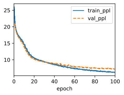
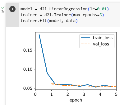
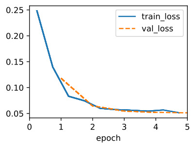
UsingThe Time Machinedataset (data), we train a character-level language model (model) based on the RNN (rnn) implemented from scratch. Note that we first calculate the gradients, then clip them, and finally update the model parameters using the clipped gradients.
Time Machine 데이터 세트(데이터)를 사용하여 처음부터 구현된 RNN(rnn)을 기반으로 문자 수준 언어 모델(모델)을 교육합니다. 먼저 그래디언트를 계산한 다음 클리핑하고 마지막으로 클리핑된 그래디언트를 사용하여 모델 매개변수를 업데이트합니다.
data = d2l.TimeMachine(batch_size=1024, num_steps=32)
rnn = RNNScratch(num_inputs=len(data.vocab), num_hiddens=32)
model = RNNLMScratch(rnn, vocab_size=len(data.vocab), lr=1)
trainer = d2l.Trainer(max_epochs=100, gradient_clip_val=1, num_gpus=1)
trainer.fit(model, data)
위 코드는 'Time Machine' 데이터셋을 사용하여 RNN 기반의 언어 모델을 학습하는 과정을 나타냅니다.
data = d2l.TimeMachine(batch_size=1024, num_steps=32): 이 코드는 'Time Machine' 데이터셋을 batch_size가 1024이고 num_steps가 32인 형태로 로드합니다. 이 데이터셋은 텍스트 데이터를 전처리하고 배치 형태로 구성하여 모델 학습에 사용될 준비를 합니다.
rnn = RNNScratch(num_inputs=len(data.vocab), num_hiddens=32): RNNScratch 클래스의 인스턴스인 rnn을 생성합니다. 이 RNN 모델은 입력 차원을 len(data.vocab)으로, 은닉 상태 차원을 32로 설정합니다.
model = RNNLMScratch(rnn, vocab_size=len(data.vocab), lr=1): RNNLMScratch 클래스의 인스턴스인 model을 생성합니다. 이 언어 모델은 앞서 생성한 rnn 모델을 기반으로 하며, 어휘 크기는 len(data.vocab)로 설정하고 학습률은 1로 설정합니다.
trainer = d2l.Trainer(max_epochs=100, gradient_clip_val=1, num_gpus=1): Trainer 클래스의 인스턴스인 trainer를 생성합니다. 이 트레이너는 최대 100 에포크 동안 학습을 수행하며, 그레디언트 클리핑 임계값을 1로 설정하고 GPU 1개를 사용하여 학습합니다.
trainer.fit(model, data): 생성한 trainer를 사용하여 모델 학습을 진행합니다. 학습 데이터는 data로 설정된 데이터셋을 사용하며, model이 학습됩니다.
요약하면, 위 코드는 'Time Machine' 데이터셋을 사용하여 RNN 기반의 언어 모델을 학습하는 과정을 나타내는 예제입니다.
9.5.5.Decoding
Once a language model has been learned, we can use it not only to predict the next token but to continue predicting each subsequent token, treating the previously predicted token as though it were the next token in the input. Sometimes we will just want to generate text as though we were starting at the beginning of a document. However, it is often useful to condition the language model on a user-supplied prefix. For example, if we were developing an autocomplete feature for search engine or to assist users in writing emails, we would want to feed in what they had written so far (the prefix), and then generate a likely continuation.
언어 모델이 학습되면 이를 사용하여 다음 토큰을 예측할 뿐만 아니라 각 후속 토큰을 계속 예측하여 이전에 예측한 토큰을 입력의 다음 토큰인 것처럼 처리할 수 있습니다. 때때로 우리는 문서의 시작 부분에서 시작하는 것처럼 텍스트를 생성하기를 원할 것입니다. 그러나 사용자가 제공한 접두사에서 언어 모델을 조건화하는 것이 종종 유용합니다. 예를 들어 검색 엔진용 자동 완성 기능을 개발하거나 사용자의 이메일 작성을 지원하는 경우 지금까지 작성한 내용(접두어)을 입력한 다음 가능성 있는 연속을 생성하려고 합니다.
The followingpredictmethod generates a continuation, one character at a time, after ingesting a user-providedprefix, When looping through the characters inprefix, we keep passing the hidden state to the next time step but do not generate any output. This is called thewarm-upperiod. After ingesting the prefix, we are now ready to begin emitting the subsequent characters, each of which will be fed back into the model as the input at the subsequent time step.
다음 예측 메서드는 사용자가 제공한 접두사를 수집한 후 한 번에 한 문자씩 연속을 생성합니다. 접두사의 문자를 통해 반복할 때 숨겨진 상태를 다음 단계로 계속 전달하지만 출력을 생성하지는 않습니다. 이것을 워밍업 기간이라고 합니다. 접두사를 수집한 후 이제 후속 문자를 방출할 준비가 되었습니다. 각 문자는 후속 시간 단계에서 입력으로 모델에 피드백됩니다.
@d2l.add_to_class(RNNLMScratch)  #@save
def predict(self, prefix, num_preds, vocab, device=None):
    state, outputs = None, [vocab[prefix[0]]]
    for i in range(len(prefix) + num_preds - 1):
        X = torch.tensor([[outputs[-1]]], device=device)
        embs = self.one_hot(X)
        rnn_outputs, state = self.rnn(embs, state)
        if i < len(prefix) - 1:  # Warm-up period
            outputs.append(vocab[prefix[i + 1]])
        else:  # Predict num_preds steps
            Y = self.output_layer(rnn_outputs)
            outputs.append(int(Y.argmax(axis=2).reshape(1)))
    return ''.join([vocab.idx_to_token[i] for i in outputs])
위 코드는 RNN 기반 언어 모델에서 주어진 접두사(prefix)와 함께 이어지는 텍스트를 생성하는 predict 메서드를 정의하는 부분입니다.
prefix: 초기 텍스트 접두사로, 이를 기반으로 이어지는 텍스트를 생성합니다.
num_preds: 생성할 텍스트의 길이를 지정합니다.
vocab: 사용할 어휘(단어 사전)를 나타냅니다.
device: 텐서 연산을 수행할 디바이스를 지정합니다. 기본값은 None으로 CPU를 사용합니다.
메서드 내부에서는 다음과 같은 절차를 수행합니다:
초기 상태(state)와 초기 출력(outputs) 리스트를 설정합니다.
주어진 접두사의 첫 번째 단어를 출력 리스트에 추가합니다.
주어진 접두사로 모델을 warm-up(사전 훈련) 시키며, 훈련된 상태와 출력을 갱신합니다.
prefix 이후로 텍스트를 생성합니다.
각 반복마다 이전 출력을 입력으로 사용하여 다음 단어를 예측합니다.
예측 결과에서 가장 높은 확률을 가진 단어를 선택하여 출력 리스트에 추가합니다.
최종적으로 출력 리스트에 추가된 단어들을 어휘의 인덱스로 변환하여 텍스트로 변환한 후 반환합니다.
이렇게 생성된 텍스트는 주어진 접두사와 모델의 예측을 조합하여 만들어진 것으로, 접두사 이후에 이어질 가능성이 높은 텍스트를 생성하는 역할을 합니다.
In the following, we specify the prefix and have it generate 20 additional characters.
위 코드는 주어진 모델을 사용하여 주어진 접두사("it has")를 기반으로 텍스트를 생성하는 과정을 수행하는 부분입니다.
model: 텍스트 생성에 사용할 RNN 기반 언어 모델입니다.
prefix: 초기 텍스트 접두사로, 이를 기반으로 이어지는 텍스트를 생성합니다.
num_preds: 생성할 텍스트의 길이를 지정합니다. 여기서는 20으로 설정되었습니다.
vocab: 사용할 어휘(단어 사전)를 나타냅니다.
device: 텐서 연산을 수행할 디바이스를 지정합니다.
이 메서드는 다음과 같이 작동합니다:
초기 상태와 출력 리스트를 설정합니다.
접두사의 각 단어를 입력으로 사용하여 초기 상태를 업데이트하고, 출력 리스트에 해당 단어를 추가합니다.
warm-up 기간 동안 입력과 초기 상태를 사용하여 모델을 훈련하고, 상태와 출력을 갱신합니다.
접두사 이후로 텍스트를 생성합니다. 각 반복마다 이전 출력을 입력으로 사용하여 다음 단어를 예측하고, 예측 결과의 가장 높은 확률을 가진 단어를 출력 리스트에 추가합니다.
출력 리스트에 있는 단어들을 어휘의 인덱스로 변환하여 생성된 텍스트를 완성합니다.
이렇게 생성된 텍스트는 주어진 접두사("it has")를 기반으로 모델이 예측한 결과로 이루어진 것입니다. 이를 통해 모델이 언어의 패턴을 이해하고, 주어진 접두사에 어울리는 텍스트를 생성하도록 학습되었음을 확인할 수 있습니다.
'it has of the the the the '
While implementing the above RNN model from scratch is instructive, it is not convenient. In the next section, we will see how to leverage deep learning frameworks to whip up RNNs using standard architectures, and to reap performance gains by relying on highly optimized library functions.
위의 RNN 모델을 처음부터 구현하는 것은 유익하지만 편리하지는 않습니다. 다음 섹션에서는 딥 러닝 프레임워크를 활용하여 표준 아키텍처를 사용하여 RNN을 강화하고 고도로 최적화된 라이브러리 기능에 의존하여 성능 향상을 얻는 방법을 살펴보겠습니다.
9.5.6.Summary
We can train RNN-based language models to generate text following the user-provided text prefix. A simple RNN language model consists of input encoding, RNN modeling, and output generation. During training, gradient clipping can mitigate the problem of exploding gradients but does not address the problem of vanishing gradients. In the experiment, we implemented a simple RNN language model and trained it with gradient clipping on sequences of text, tokenized at the character level. By conditioning on a prefix, we can use a language model to generate likely continuations, which proves useful in many applications, e.g., autocomplete features.
사용자가 제공한 텍스트 접두사 다음에 텍스트를 생성하도록 RNN 기반 언어 모델을 훈련할 수 있습니다. 간단한 RNN 언어 모델은 입력 인코딩, RNN 모델링 및 출력 생성으로 구성됩니다. 교육 중에 그래디언트 클리핑은 그래디언트 폭발 문제를 완화할 수 있지만 그래디언트 소실 문제는 해결하지 못합니다. 실험에서 간단한 RNN 언어 모델을 구현하고 문자 수준에서 토큰화된 텍스트 시퀀스에서 그래디언트 클리핑으로 학습했습니다. 접두사를 조건으로 하여 언어 모델을 사용하여 가능한 연속을 생성할 수 있으며, 이는 자동 완성 기능과 같은 많은 응용 프로그램에서 유용합니다.
9.5.7.Exercises
Does the implemented language model predict the next token based on all the past tokens up to the very first token inThe Time Machine?
Which hyperparameter controls the length of history used for prediction?
Show that one-hot encoding is equivalent to picking a different embedding for each object.
Adjust the hyperparameters (e.g., number of epochs, number of hidden units, number of time steps in a minibatch, and learning rate) to improve the perplexity. How low can you go while sticking with this simple architecture?
Replace one-hot encoding with learnable embeddings. Does this lead to better performance?
Conduct an experiment to determine how well this language model trained onThe Time Machineworks on other books by H. G. Wells, e.g.,The War of the Worlds.
Conduct another experiment to evaluate the perplexity of this model on books written by other authors.
InSection 9.3we described Markov models andn-grams for language modeling, where the conditional probability of tokenxtat time steptonly depends on then−1previous tokens. If we want to incorporate the possible effect of tokens earlier than time stept−(n−1)onxt, we need to increasen. However, the number of model parameters would also increase exponentially with it, as we need to store|V|nnumbers for a vocabulary setV. Hence, rather than modelingP(xt∣xt−1,…,xt−n+1)it is preferable to use a latent variable model:
섹션 9.3에서 우리는 언어 모델링을 위한 Markov 모델과 n-그램을 설명했습니다. 여기서 시간 단계 t에서 토큰 xt의 조건부 확률은 n-1 이전 토큰에만 의존합니다. xt에 대한 시간 단계 t-(n-1) 이전의 토큰의 가능한 효과를 통합하려면 n을 증가시켜야 합니다. 그러나 어휘 집합 V에 대해 |V|n 숫자를 저장해야 하므로 모델 매개변수의 수도 기하급수적으로 증가합니다. 따라서 P(xt∣xt−1,…,xt−n+1을 모델링하는 대신 ) 잠재 변수 모델을 사용하는 것이 바람직합니다.
whereℎt−1is ahidden statethat stores the sequence information up to time stept−1. In general, the hidden state at any time steptcould be computed based on both the current inputxtand the previous hidden stateℎt−1:
여기서 ℎt-1은 시간 단계 t-1까지의 시퀀스 정보를 저장하는 숨겨진 상태입니다. 일반적으로 t단계의 숨겨진 상태는 현재 입력 xt와 이전 숨겨진 상태 ℎt-1을 기반으로 계산할 수 있습니다.
For a sufficiently powerful functionfin(9.4.2), the latent variable model is not an approximation. After all,ℎtmay simply store all the data it has observed so far. However, it could potentially make both computation and storage expensive.
(9.4.2)의 충분히 강력한 함수 f의 경우 잠재 변수 모델은 근사치가 아닙니다. 결국 ℎt는 지금까지 관찰한 모든 데이터를 단순히 저장할 수 있습니다. 그러나 잠재적으로 계산과 저장 비용이 모두 비쌀 수 있습니다.
Recall that we have discussed hidden layers with hidden units inSection 5. It is noteworthy that hidden layers and hidden states refer to two very different concepts. Hidden layers are, as explained, layers that are hidden from view on the path from input to output. Hidden states are technically speakinginputsto whatever we do at a given step, and they can only be computed by looking at data at previous time steps.
섹션 5에서 은닉 유닛이 있는 은닉층에 대해 논의한 것을 상기하십시오. 은닉층과 은닉 상태는 매우 다른 두 가지 개념을 나타냅니다. 숨겨진 레이어는 설명된 대로 입력에서 출력까지의 경로에서 보기에서 숨겨진 레이어입니다. 숨겨진 상태는 기술적으로 주어진 단계에서 수행하는 모든 작업에 대한 입력이며 이전 시간 단계의 데이터를 확인해야만 계산할 수 있습니다.
Recurrent neural networks(RNNs) are neural networks with hidden states. Before introducing the RNN model, we first revisit the MLP model introduced inSection 5.1.
순환 신경망(RNN)은 숨겨진 상태가 있는 신경망입니다. RNN 모델을 소개하기 전에 먼저 섹션 5.1에서 소개한 MLP 모델을 다시 살펴보겠습니다.
import torch
from d2l import torch as d2l
9.4.1.Neural Networks without Hidden States
Let’s take a look at an MLP with a single hidden layer. Let the hidden layer’s activation function beϕ. Given a minibatch of examplesX∈Rn×dwith batch sizenanddinputs, the hidden layer outputH∈Rn×ℎis calculated as
단일 히든 레이어가 있는 MLP를 살펴보겠습니다. 은닉층의 활성화 함수를 φ라 하자. 배치 크기가 n이고 입력이 d인 예제 X∈Rn×d의 미니 배치가 주어지면 숨겨진 계층 출력 H∈Rn×ℎ는 다음과 같이 계산됩니다.
In(9.4.3), we have the weight parameterWxℎ∈Rd×ℎ, the bias parameterbℎ∈R1×ℎ, and the number of hidden unitsℎ, for the hidden layer. Thus, broadcasting (seeSection 2.1.4) is applied during the summation. Next, the hidden layer outputHis used as input of the output layer. The output layer is given by
(9.4.3)에서 은닉 계층에 대한 가중치 매개변수 Wxℎ∈Rd×ℎ, 편향 매개변수 bℎ∈R1×ℎ 및 은닉 유닛의 수 ℎ가 있습니다. 따라서 브로드캐스팅(섹션 2.1.4 참조)은 합산 중에 적용됩니다. 다음으로 숨겨진 레이어 출력 H는 출력 레이어의 입력으로 사용됩니다. 출력 레이어는 다음과 같이 지정됩니다.
whereO∈Rn×qis the output variable,Wℎq∈Rℎ×qis the weight parameter, andbq∈R1×qis the bias parameter of the output layer. If it is a classification problem, we can usesoftmax(O)to compute the probability distribution of the output categories.
여기서 O∈Rn×q는 출력 변수, Wℎq∈Rℎ×q는 가중치 매개변수, bq∈R1×q는 출력 레이어의 편향 매개변수입니다. 분류 문제인 경우 softmax(O)를 사용하여 출력 범주의 확률 분포를 계산할 수 있습니다.
This is entirely analogous to the regression problem we solved previously inSection 9.1, hence we omit details. Suffice it to say that we can pick feature-label pairs at random and learn the parameters of our network via automatic differentiation and stochastic gradient descent.
이것은 섹션 9.1에서 이전에 해결한 회귀 문제와 완전히 유사하므로 세부 사항을 생략합니다. 기능 레이블 쌍을 무작위로 선택하고 자동 미분 및 확률적 경사 하강법을 통해 네트워크의 매개변수를 학습할 수 있다고 말하는 것으로 충분합니다.
Hidden Layer와 Hidden State.
In the context of Recurrent Neural Networks (RNNs), both "hidden layer" and "hidden state" are terms that refer to specific concepts within the architecture of the network. However, they represent different aspects of how information is processed and propagated through the network.
RNN(순환 신경망)의 맥락에서 "은닉 레이어(hidden layer)"와 "은닉 상태(hidden state)"는 네트워크의 아키텍처 내에서 특정 개념을 나타내는 용어입니다. 그러나 이들은 정보가 어떻게 처리되고 전달되는지에 대한 다른 측면을 나타냅니다.
Hidden Layer: The term "hidden layer" in an RNN generally refers to the layer of neurons that exist between the input layer and the output layer. These neurons are responsible for capturing and transforming the input data into a format that is suitable for making predictions or generating outputs. In the case of an RNN, the hidden layer is the part of the network where the temporal or sequential information is captured. Each neuron in the hidden layer takes as input the data from the input layer and its own previous state, and produces an output that is then passed to the next time step. Essentially, the hidden layer processes input data and passes relevant information forward through time.
RNN의 "은닉 레이어"는 일반적으로 입력 레이어와 출력 레이어 사이에 있는 뉴런의 레이어를 가리킵니다. 이러한 뉴런은 입력 데이터를 적절한 형식으로 변환하고 변환하는 역할을 담당합니다. RNN의 경우 은닉 레이어는 시간적 또는 순차적 정보가 포착되는 부분입니다. 은닉 레이어의 각 뉴런은 입력 레이어의 데이터와 이전 상태를 입력으로 받아들이고 다음 시간 단계로 전달될 출력을 생성합니다. 기본적으로 은닉 레이어는 입력 데이터를 처리하고 관련 정보를 시간을 통해 전달합니다.
Hidden State: The "hidden state," on the other hand, refers specifically to the output that is generated by the hidden layer of an RNN at a particular time step. It contains the processed information that the RNN has learned from the sequence of inputs up to that point. This hidden state is then used as input for the next time step, along with the input data at that time step. In essence, the hidden state encapsulates the network's memory or understanding of the sequence up to the current time step.
반면에 "은닉 상태"는 특정 시간 단계에서 RNN의 은닉 레이어가 생성하는 출력을 지칭합니다. 이 은닉 상태는 해당 지점까지의 입력 시퀀스로부터 학습한 처리된 정보를 포함합니다. 이 은닉 상태는 다음 시간 단계의 입력과 함께 다음 시간 단계로 전달됩니다. 본질적으로 은닉 상태는 네트워크의 메모리 또는 현재 시간 단계까지의 시퀀스를 나타내며 다음 시간 단계의 입력 역할을 합니다.
In summary, the hidden layer is a conceptual layer within the architecture of the RNN that performs computations to process and transform input data over time, while the hidden state is the actual output or representation produced by the hidden layer at a specific time step, which serves as both the network's memory and input for the next time step.
요약하면, 은닉 레이어는 RNN 아키텍처 내에서 계산을 수행하여 시간에 따라 입력 데이터를 처리하고 변환하는 개념적인 레이어입니다. 반면 은닉 상태는 특정 시간 단계에서 은닉 레이어가 생성하는 실제 출력 또는 표현이며 네트워크의 메모리 역할과 다음 시간 단계의 입력 역할을 동시에 수행합니다.
9.4.2.Recurrent Neural Networks with Hidden States
Matters are entirely different when we have hidden states. Let’s look at the structure in some more detail.
숨겨진 상태가 있을 때는 문제가 완전히 다릅니다. 구조를 좀 더 자세히 살펴보겠습니다.
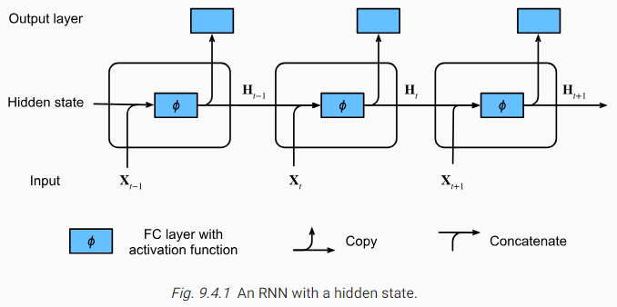
Assume that we have a minibatch of inputsXt∈Rn×dat time step t. In other words, for a minibatch ofnsequence examples, each row ofXtcorresponds to one example at time steptfrom the sequence. Next, denote byHt∈Rn×ℎthe hidden layer output of time stept. Unlike the MLP, here we save the hidden layer outputHt−1from the previous time step and introduce a new weight parameterWℎℎ∈Rℎ×ℎto describe how to use the hidden layer output of the previous time step in the current time step. Specifically, the calculation of the hidden layer output of the current time step is determined by the input of the current time step together with the hidden layer output of the previous time step:
시간 단계 t에서 입력 Xt∈Rn×d의 미니배치가 있다고 가정합니다. 다시 말해, n 시퀀스 예제의 미니배치에 대해 Xt의 각 행은 시퀀스의 시간 단계 t에서 하나의 예제에 해당합니다. 다음으로 시간 단계 t의 숨겨진 레이어 출력을 Ht∈Rn×ℎ로 표시합니다. MLP와 달리 여기서는 이전 시간 단계의 숨겨진 계층 출력 Ht-1을 저장하고 현재 시간 단계에서 이전 시간 단계의 숨겨진 계층 출력을 사용하는 방법을 설명하기 위해 새로운 가중치 매개변수 Wℎℎ∈Rℎ×ℎ를 도입합니다. 특히, 현재 시간 단계의 은닉층 출력 계산은 이전 시간 단계의 은닉층 출력과 함께 현재 시간 단계의 입력에 의해 결정됩니다.
Compared with(9.4.3),(9.4.5)adds one more termHt−1Wℎℎand thus instantiates(9.4.2). From the relationship between hidden layer outputsHtandHt−1of adjacent time steps, we know that these variables captured and retained the sequence’s historical information up to their current time step, just like the state or memory of the neural network’s current time step. Therefore, such a hidden layer output is called ahidden state. Since the hidden state uses the same definition of the previous time step in the current time step, the computation of(9.4.5)isrecurrent. Hence, as we said, neural networks with hidden states based on recurrent computation are namedrecurrent neural networks. Layers that perform the computation of(9.4.5)in RNNs are calledrecurrent layers.
(9.4.3)과 비교하여 (9.4.5)는 Ht−1Wℎℎ 항을 하나 더 추가하여 (9.4.2)를 인스턴스화합니다. 인접한 시간 단계의 숨겨진 레이어 출력 Ht와 Ht-1 사이의 관계에서 우리는 이러한 변수가 신경망의 현재 시간 단계의 상태 또는 메모리와 마찬가지로 현재 시간 단계까지 시퀀스의 과거 정보를 캡처하고 유지한다는 것을 알고 있습니다. 따라서 이러한 은닉층 출력을 은닉 상태(hidden state)라고 합니다. 숨겨진 상태는 현재 시간 단계에서 이전 시간 단계의 동일한 정의를 사용하므로 (9.4.5)의 계산이 반복됩니다. 따라서 우리가 말했듯이 순환 계산을 기반으로 하는 숨겨진 상태가 있는 신경망을 순환 신경망이라고 합니다. RNN에서 (9.4.5)의 계산을 수행하는 계층을 순환 계층이라고 합니다.
There are many different ways for constructing RNNs. RNNs with a hidden state defined by(9.4.5)are very common. For time stept, the output of the output layer is similar to the computation in the MLP:
RNN을 구성하는 방법에는 여러 가지가 있습니다. (9.4.5)로 정의된 숨겨진 상태가 있는 RNN은 매우 일반적입니다. 시간 단계 t의 경우 출력 계층의 출력은 MLP의 계산과 유사합니다.
Parameters of the RNN include the weightsWxℎ∈Rd×ℎ,Wℎℎ∈Rℎ×ℎ, and the biasbℎ∈R1×ℎof the hidden layer, together with the weightsWℎq∈Rℎ×qand the biasbq∈R1×qof the output layer. It is worth mentioning that even at different time steps, RNNs always use these model parameters. Therefore, the parameterization cost of an RNN does not grow as the number of time steps increases.
RNN의 파라미터에는 가중치 Wxℎ∈Rd×ℎ, Wℎℎ∈Rℎ×ℎ, 숨겨진 레이어의 바이어스 bℎ∈R1×ℎ, 가중치 Wℎq∈Rℎ×q 및 바이어스 bq∈R1×q가 포함됩니다. 출력 레이어. 다른 시간 단계에서도 RNN은 항상 이러한 모델 매개변수를 사용한다는 점을 언급할 가치가 있습니다. 따라서 RNN의 매개변수화 비용은 시간 단계가 증가해도 증가하지 않습니다.
Fig. 9.4.1illustrates the computational logic of an RNN at three adjacent time steps. At any time stept, the computation of the hidden state can be treated as: (i) concatenating the inputXtat the current time steptand the hidden stateHt−1at the previous time stept−1; (ii) feeding the concatenation result into a fully connected layer with the activation functionϕ. The output of such a fully connected layer is the hidden stateHtof the current time stept. In this case, the model parameters are the concatenation ofWxℎandWℎℎ, and a bias ofbℎ, all from(9.4.5). The hidden state of the current time stept,Ht, will participate in computing the hidden stateHt+1of the next time stept+1. What is more,Htwill also be fed into the fully connected output layer to compute the outputOtof the current time stept.
그림 9.4.1은 세 개의 인접한 시간 단계에서 RNN의 계산 논리를 보여줍니다. 임의의 시간 단계 t에서 숨겨진 상태의 계산은 다음과 같이 처리될 수 있습니다. (i) 현재 시간 단계 t의 입력 Xt와 이전 시간 단계 t-1의 숨겨진 상태 Ht-1을 연결합니다. (ii) 연결 결과를 활성화 함수 φ와 함께 완전히 연결된 레이어에 공급합니다. 이러한 완전 연결 계층의 출력은 현재 시간 단계 t의 숨겨진 상태 Ht입니다. 이 경우 모델 매개변수는 모두 (9.4.5)에서 Wxℎ와 Wℎℎ의 연결과 bℎ의 바이어스입니다. 현재 시간 단계 t의 은닉 상태인 Ht는 다음 시간 단계 t+1의 은닉 상태 Ht+1을 계산하는 데 참여합니다. 또한 Ht는 현재 시간 단계 t의 출력 Ot를 계산하기 위해 완전히 연결된 출력 계층에 공급됩니다.
We just mentioned that the calculation of XtWxℎ+Ht−1Wℎℎfor the hidden state is equivalent to matrix multiplication of concatenation ofXtandHt−1and concatenation ofWxℎandWℎℎ. Though this can be proven in mathematics, in the following we just use a simple code snippet to show this. To begin with, we define matricesX,W_xh,H, andW_hh, whose shapes are (3, 1), (1, 4), (3, 4), and (4, 4), respectively. MultiplyingXbyW_xh, andHbyW_hh, respectively, and then adding these two multiplications, we obtain a matrix of shape (3, 4).
은닉 상태에 대한 XtWxℎ+Ht−1Wℎℎ의 계산은 Xt와 Ht−1의 연결 및 Wxℎ와 Wℎℎ의 연결의 행렬 곱셈과 동일하다고 언급했습니다. 이것은 수학에서 증명될 수 있지만 다음에서는 이를 보여주기 위해 간단한 코드 스니펫을 사용합니다. 우선, 모양이 각각 (3, 1), (1, 4), (3, 4) 및 (4, 4)인 행렬 X, W_xh, H 및 W_hh를 정의합니다. X에 W_xh를 곱하고 H에 W_hh를 각각 곱한 다음 이 두 곱을 더하면 모양이 (3, 4)인 행렬을 얻습니다.
Now we concatenate the matricesXandHalong columns (axis 1), and the matricesW_xhandW_hhalong rows (axis 0). These two concatenations result in matrices of shape (3, 5) and of shape (5, 4), respectively. Multiplying these two concatenated matrices, we obtain the same output matrix of shape (3, 4) as above.
이제 열(축 1)을 따라 행렬 X와 H를 연결하고 행(축 0)을 따라 행렬 W_xh와 W_hh를 연결합니다. 이 두 연결은 각각 형태 (3, 5) 및 형태 (5, 4)의 행렬을 생성합니다. 이 두 개의 연결된 행렬을 곱하면 위와 같은 (3, 4) 모양의 동일한 출력 행렬을 얻습니다.
위 코드는 두 개의 입력을 연결하고 이에 대해 가중치 행렬의 곱을 계산하는 과정을 나타냅니다. 이 코드는 순환 신경망(RNN)에서 입력과 이전 숨겨진 상태를 함께 고려하여 새로운 숨겨진 상태를 계산하는 것을 표현합니다.
여기서 X는 입력 벡터, H는 현재 숨겨진 상태 벡터입니다. 두 개의 행렬을 각각 가로 방향으로 연결하고, 연결된 행렬에 가중치 행렬의 곱을 수행합니다.
torch.cat((X, H), 1)은 입력 벡터 X와 현재 숨겨진 상태 벡터 H를 가로 방향으로 연결한 행렬을 생성합니다. 마찬가지로, torch.cat((W_xh, W_hh), 0)은 입력에서 숨겨진 상태로의 가중치 행렬 W_xh와 숨겨진 상태에서 다음 숨겨진 상태로의 가중치 행렬 W_hh를 세로 방향으로 연결한 행렬을 생성합니다.
연결된 입력과 가중치 행렬을 곱하면, 입력과 이전 숨겨진 상태를 고려한 새로운 숨겨진 상태가 계산됩니다. 이러한 과정은 RNN에서 시퀀스 데이터를 처리하고 이전 상태의 정보를 유지하는 데 사용됩니다.
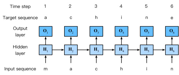
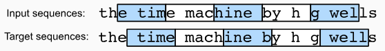
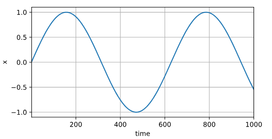
Recall that for language modeling inSection 9.3, we aim to predict the next token based on the current and past tokens, thus we shift the original sequence by one token as the targets (labels).Bengioet al.(2003)first proposed to use a neural network for language modeling. In the following we illustrate how RNNs can be used to build a language model. Let the minibatch size be one, and the sequence of the text be “machine”. To simplify training in subsequent sections, we tokenize text into characters rather than words and consider acharacter-level language model.Fig. 9.4.2demonstrates how to predict the next character based on the current and previous characters via an RNN for character-level language modeling.
섹션 9.3의 언어 모델링의 경우 현재 및 과거 토큰을 기반으로 다음 토큰을 예측하는 것을 목표로 하므로 원래 시퀀스를 대상(레이블)으로 한 토큰만큼 이동합니다. Bengioet al. (2003)은 언어 모델링을 위해 신경망을 사용하는 것을 처음 제안했습니다. 다음에서는 RNN을 사용하여 언어 모델을 구축하는 방법을 설명합니다. 미니 배치 크기를 1로 하고 텍스트의 순서를 "machine"로 설정합니다. 후속 섹션에서 교육을 단순화하기 위해 텍스트를 단어가 아닌 문자로 토큰화하고 문자 수준 언어 모델을 고려합니다. 그림 9.4.2는 문자 수준 언어 모델링을 위해 RNN을 통해 현재 및 이전 문자를 기반으로 다음 문자를 예측하는 방법을 보여줍니다.
Fig. 9.4.2 A character-level language model based on the RNN. The input and target sequences are “machin” and “achine”, respectively.
During the training process, we run a softmax operation on the output from the output layer for each time step, and then use the cross-entropy loss to compute the error between the model output and the target. Due to the recurrent computation of the hidden state in the hidden layer, the output of time step 3 inFig. 9.4.2,O3, is determined by the text sequence “m”, “a”, and “c”. Since the next character of the sequence in the training data is “h”, the loss of time step 3 will depend on the probability distribution of the next character generated based on the feature sequence “m”, “a”, “c” and the target “h” of this time step.
training 프로세스 중에 각 시간 단계에 대해 출력 레이어의 출력에 대해 소프트맥스 작업을 실행한 다음 교차 엔트로피 손실을 사용하여 모델 출력과 대상 간의 오류를 계산합니다. 은닉층에서 은닉 상태의 반복 계산으로 인해 그림 9.4.2의 시간 단계 3인 O3의 출력은 텍스트 시퀀스 "m", "a" 및 "c"에 의해 결정됩니다. 학습 데이터에서 시퀀스의 다음 문자가 "h"이므로 시간 단계 3의 손실은 특징 시퀀스 "m", "a", "c" 및 이 시간 단계의 목표 "h".
In practice, each token is represented by ad-dimensional vector, and we use a batch sizen>1. Therefore, the inputXtat time steptwill be an×dmatrix, which is identical to what we discussed inSection 9.4.2.
실제로 각 토큰은 d차원 벡터로 표현되며 배치 크기 n>1을 사용합니다. 따라서 시간 단계 t에서의 입력 Xt는 n×d 행렬이 될 것이며 이는 섹션 9.4.2에서 논의한 것과 동일합니다.
In the following sections, we will implement RNNs for character-level language models.
다음 섹션에서는 문자 수준 언어 모델을 위한 RNN을 구현합니다.
9.4.4.Summary
A neural network that uses recurrent computation for hidden states is called a recurrent neural network (RNN). The hidden state of an RNN can capture historical information of the sequence up to the current time step. With recurrent computation, the number of RNN model parameters does not grow as the number of time steps increases. As for applications, an RNN can be used to create character-level language models.
은닉 상태에 대해 반복 계산을 사용하는 신경망을 순환 신경망(RNN)이라고 합니다. RNN의 숨겨진 상태는 현재 시간 단계까지 시퀀스의 과거 정보를 캡처할 수 있습니다. 반복 계산을 사용하면 RNN 모델 매개변수의 수는 시간 단계의 수가 증가해도 증가하지 않습니다. 애플리케이션의 경우 RNN을 사용하여 문자 수준 언어 모델을 만들 수 있습니다.
9.4.5.Exercises
If we use an RNN to predict the next character in a text sequence, what is the required dimension for any output?
Why can RNNs express the conditional probability of a token at some time step based on all the previous tokens in the text sequence?
What happens to the gradient if you backpropagate through a long sequence?
What are some of the problems associated with the language model described in this section?
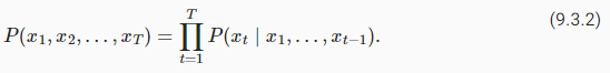
InSection 9.2, we see how to map text sequences into tokens, where these tokens can be viewed as a sequence of discrete observations, such as words or characters. Assume that the tokens in a text sequence of lengthTare in turnx1,x2,…,xT. The goal oflanguage modelsis to estimate the joint probability of the whole sequence:
섹션 9.2에서는 텍스트 시퀀스를 토큰으로 매핑하는 방법을 살펴봅니다. 여기서 이러한 토큰은 단어나 문자와 같은 개별 관찰 시퀀스로 볼 수 있습니다. 길이가 T인 텍스트 시퀀스의 토큰이 차례로 x1,x2,…,xT라고 가정합니다. 언어 모델의 목표는 전체 시퀀스의 결합 확률을 추정하는 것입니다.
where statistical tools inSection 9.1can be applied.
섹션 9.1의 통계 도구를 적용할 수 있습니다.
Language models are incredibly useful. For instance, an ideal language model would be able to generate natural text just on its own, simply by drawing one token at a time xt∼P(xt∣xt−1,…,x1). Quite unlike the monkey using a typewriter, all text emerging from such a model would pass as natural language, e.g., English text. Furthermore, it would be sufficient for generating a meaningful dialog, simply by conditioning the text on previous dialog fragments. Clearly we are still very far from designing such a system, since it would need tounderstandthe text rather than just generate grammatically sensible content.
언어 모델은 매우 유용합니다. 예를 들어, 이상적인 언어 모델은 한 번에 하나의 토큰 xt∼P(xt∣xt−1,…,x1)을 그리는 것만으로 자체적으로 자연 텍스트를 생성할 수 있습니다. 타자기를 사용하는 원숭이와는 달리 이러한 모델에서 나오는 모든 텍스트는 자연어(예: 영어 텍스트)로 전달됩니다. 또한 이전 대화 조각에서 텍스트를 조건화하는 것만으로 의미 있는 대화를 생성하는 데 충분합니다. 분명히 우리는 그러한 시스템을 설계하는 것과는 거리가 멀다. 문법적으로 의미 있는 콘텐츠를 생성하는 것보다 텍스트를 이해해야 하기 때문이다.
Nonetheless, language models are of great service even in their limited form. For instance, the phrases “to recognize speech” and “to wreck a nice beach” sound very similar. This can cause ambiguity in speech recognition, which is easily resolved through a language model that rejects the second translation as outlandish. Likewise, in a document summarization algorithm it is worthwhile knowing that “dog bites man” is much more frequent than “man bites dog”, or that “I want to eat grandma” is a rather disturbing statement, whereas “I want to eat, grandma” is much more benign.
그럼에도 불구하고 언어 모델은 제한된 형식에서도 훌륭한 서비스를 제공합니다. 예를 들어, "to recognize speech"와 "to wreck a nice beach"라는 문구는 매우 비슷하게 들립니다. 이로 인해 음성 인식에서 모호성이 발생할 수 있으며, 두 번째 번역을 이상하다고 거부하는 언어 모델을 통해 쉽게 해결됩니다. 마찬가지로 문서 요약 알고리즘에서 "dog bites man"가 "man bites dog"보다 훨씬 더 자주 발생하거나 "I want to eat grandma"는 다소 불안한 진술인 반면 "I want to eat, grandma”가 훨씬 더 온화합니다.
import torch
from d2l import torch as d2l
9.3.1.Learning Language Models
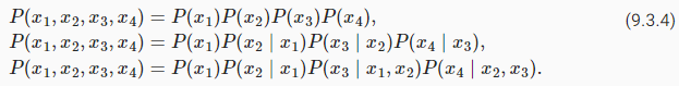
The obvious question is how we should model a document, or even a sequence of tokens. Suppose that we tokenize text data at the word level. Let’s start by applying basic probability rules:
분명한 질문은 어떻게 문서 또는 일련의 토큰을 모델링하는가 하는겁니다. 단어 수준에서 텍스트 데이터를 토큰화한다고 가정합니다. 기본 확률 규칙을 적용하여 시작하겠습니다.
For example, the probability of a text sequence containing four words would be given as:
예를 들어, 4개의 단어를 포함하는 텍스트 시퀀스의 확률은 다음과 같이 주어집니다.
9.3.1.1.Markov Models and n-grams
Among those sequence model analysis inSection 9.1, let’s apply Markov models to language modeling. A distribution over sequences satisfies the Markov property of first order ifP(xt+1∣xt,…,x1)=P(xt+1∣xt). Higher orders correspond to longer dependencies. This leads to a number of approximations that we could apply to model a sequence:
9.1절의 시퀀스 모델 분석 중 Markov 모델을 언어 모델링에 적용해 보자. 시퀀스에 대한 분포는 P(xt+1∣xt,…,x1)=P(xt+1∣xt)인 경우 1차 Markov 속성을 만족합니다. 더 높은 차수는 더 긴 종속성에 해당합니다. 이는 시퀀스를 모델링하는 데 적용할 수 있는 여러 가지 근사치로 이어집니다.
The probability formulae that involve one, two, and three variables are typically referred to asunigram,bigram, andtrigrammodels, respectively. In order to compute the language model, we need to calculate the probability of words and the conditional probability of a word given the previous few words. Note that such probabilities are language model parameters.
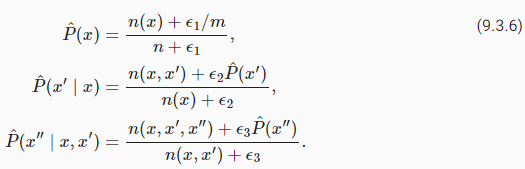
1개, 2개 및 3개의 변수를 포함하는 확률 공식은 일반적으로 각각 유니그램, 바이그램 및 트라이그램 모델이라고 합니다. 언어 모델을 계산하기 위해서는 단어의 확률과 이전 몇 단어가 주어진 단어의 조건부 확률을 계산해야 합니다. 이러한 확률은 언어 모델 매개변수입니다.
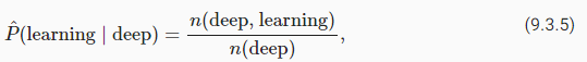
9.3.1.2.Word Frequency
Here, we assume that the training dataset is a large text corpus, such as all Wikipedia entries,Project Gutenberg, and all text posted on the Web. The probability of words can be calculated from the relative word frequency of a given word in the training dataset. For example, the estimateP^(deep)can be calculated as the probability of any sentence starting with the word “deep”. A slightly less accurate approach would be to count all occurrences of the word “deep” and divide it by the total number of words in the corpus. This works fairly well, particularly for frequent words. Moving on, we could attempt to estimate wheren(x)andn(x,x′)are the number of occurrences of singletons and consecutive word pairs, respectively.
여기서는 교육 데이터 세트가 모든 Wikipedia 항목, Project Gutenberg 및 웹에 게시된 모든 텍스트와 같은 대규모 텍스트 코퍼스라고 가정합니다. 단어의 확률은 훈련 데이터 세트에서 주어진 단어의 상대적인 단어 빈도에서 계산할 수 있습니다. 예를 들어 추정치 P^(deep)는 "deep"이라는 단어로 시작하는 문장의 확률로 계산할 수 있습니다. 약간 덜 정확한 접근 방식은 "deep"이라는 단어의 모든 발생을 세고 이를 말뭉치의 총 단어 수로 나누는 것입니다. 이것은 특히 빈번한 단어에 대해 상당히 잘 작동합니다. 계속해서 n(x) 및 n(x,x′)가 각각 싱글톤 및 연속 단어 쌍의 발생 횟수인 추정을 시도할 수 있습니다.
Unfortunately, estimating the probability of a word pair is somewhat more difficult, since the occurrences of “deep learning” are a lot less frequent. In particular, for some unusual word combinations it may be tricky to find enough occurrences to get accurate estimates. As suggested by the empirical results inSection 9.2.5, things take a turn for the worse for three-word combinations and beyond. There will be many plausible three-word combinations that we likely will not see in our dataset. Unless we provide some solution to assign such word combinations nonzero count, we will not be able to use them in a language model. If the dataset is small or if the words are very rare, we might not find even a single one of them.
불행히도 "딥 러닝"의 발생 빈도가 훨씬 적기 때문에 단어 쌍의 확률을 추정하는 것은 다소 어렵습니다. 특히 일부 비정상적인 단어 조합의 경우 정확한 추정치를 얻기에 충분한 항목을 찾는 것이 까다로울 수 있습니다. 섹션 9.2.5의 실증적 결과에서 제안한 것처럼 세 단어 조합 이상에서는 상황이 악화됩니다. 데이터 세트에서 볼 수 없는 그럴듯한 3단어 조합이 많이 있을 것입니다. 이러한 단어 조합을 0이 아닌 개수로 지정하는 솔루션을 제공하지 않는 한 언어 모델에서 사용할 수 없습니다. 데이터 세트가 작거나 단어가 매우 드문 경우 하나도 찾지 못할 수 있습니다.
9.3.1.3.Laplace Smoothing
A common strategy is to perform some form ofLaplace smoothing. The solution is to add a small constant to all counts. Denote bynthe total number of words in the training set andmthe number of unique words. This solution helps with singletons, e.g., via
일반적인 전략은 어떤 형태의 Laplace smoothing을 수행하는 것입니다. 해결책은 모든 카운트에 작은 상수를 추가하는 것입니다. 훈련 세트의 총 단어 수를 n으로 표시하고 고유 단어 수를 m으로 표시합니다. 이 솔루션은 예를 들어 다음을 통해 싱글톤에 도움이 됩니다.
Hereϵ1,ϵ2, andϵ3are hyperparameters. Takeϵ1as an example: whenϵ1=0, no smoothing is applied; whenϵ1approaches positive infinity,P^(x)approaches the uniform probability1/m. The above is a rather primitive variant of what other techniques can accomplish(Woodet al., 2011).
여기서 ϵ1, ϵ2 및 ϵ3은 하이퍼파라미터입니다. ϵ1을 예로 들어 보겠습니다. ϵ1=0이면 스무딩이 적용되지 않습니다. ϵ1이 양의 무한대에 접근하면 P^(x)는 균일 확률 1/m에 접근합니다. 위의 내용은 다른 기술이 수행할 수 있는 것의 다소 원시적인 변형입니다(Wood et al., 2011).
Unfortunately, models like this get unwieldy rather quickly for the following reasons. First, as discussed inSection 9.2.5, manyn-grams occur very rarely, making Laplace smoothing rather unsuitable for language modeling. Second, we need to store all counts. Third, this entirely ignores the meaning of the words. For instance, “cat” and “feline” should occur in related contexts. It is quite difficult to adjust such models to additional contexts, whereas, deep learning based language models are well suited to take this into account. Last, long word sequences are almost certain to be novel, hence a model that simply counts the frequency of previously seen word sequences is bound to perform poorly there. Therefore, we focus on using neural networks for language modeling in the rest of the chapter.
불행하게도 이와 같은 모델은 다음과 같은 이유로 다소 빨리 다루기 어려워집니다. 첫째, 섹션 9.2.5에서 논의한 것처럼 많은 n-gram이 매우 드물게 발생하므로 Laplace smoothing는 언어 모델링에 적합하지 않습니다. 둘째, 모든 카운트를 저장해야 합니다. 셋째, 이것은 단어의 의미를 완전히 무시합니다. 예를 들어, "cat"과 "feline"은 관련 문맥에서 발생해야 합니다. 이러한 모델을 추가 컨텍스트에 맞게 조정하는 것은 매우 어려운 반면 딥 러닝 기반 언어 모델은 이를 고려하는 데 적합합니다. 마지막으로, 긴 단어 시퀀스는 새로운 것이 거의 확실하므로 이전에 본 단어 시퀀스의 빈도를 단순히 세는 모델은 성능이 좋지 않을 수 밖에 없습니다. 따라서 나머지 장에서는 언어 모델링을 위해 신경망을 사용하는 데 중점을 둡니다.
9.3.2.Perplexity
Next, let’s discuss about how to measure the language model quality, which will be used to evaluate our models in the subsequent sections. One way is to check how surprising the text is. A good language model is able to predict with high-accuracy tokens that what we will see next. Consider the following continuations of the phrase “It is raining”, as proposed by different language models:
다음으로, 후속 섹션에서 모델을 평가하는 데 사용될 언어 모델 품질을 측정하는 방법에 대해 논의하겠습니다. 한 가지 방법은 텍스트가 얼마나 놀라운지 확인하는 것입니다. 좋은 언어 모델은 우리가 다음에 보게 될 것을 높은 정확도의 토큰으로 예측할 수 있습니다. 다른 언어 모델에서 제안한 대로 "It is raining"이라는 구문의 다음 연속을 고려하십시오.
“It is raining outside”
“It is raining banana tree”
“It is raining piouw;kcj pwepoiut”
In terms of quality, example 1 is clearly the best. The words are sensible and logically coherent. While it might not quite accurately reflect which word follows semantically (“in San Francisco” and “in winter” would have been perfectly reasonable extensions), the model is able to capture which kind of word follows. Example 2 is considerably worse by producing a nonsensical extension. Nonetheless, at least the model has learned how to spell words and some degree of correlation between words. Last, example 3 indicates a poorly trained model that does not fit data properly.
품질면에서는 예제 1이 확실히 최고입니다. 단어가 합리적이고 논리적으로 일관성이 있습니다. 어떤 단어가 의미론적으로 뒤따르는지 정확히 반영하지 못할 수도 있지만("in San Francisco"와 "in winter"는 완벽하게 합리적인 확장이었을 것입니다), 모델은 어떤 종류의 단어가 뒤에 오는지 캡처할 수 있습니다. 예제 2는 무의미한 확장을 생성하여 상당히 더 나쁩니다. 그럼에도 불구하고 적어도 모델은 단어의 철자와 단어 간의 상관 관계를 어느 정도 배웠습니다. 마지막으로 예제 3은 데이터를 제대로 맞추지 못하는 제대로 훈련되지 않은 모델을 나타냅니다.
We might measure the quality of the model by computing the likelihood of the sequence. Unfortunately this is a number that is hard to understand and difficult to compare. After all, shorter sequences are much more likely to occur than the longer ones, hence evaluating the model on Tolstoy’s magnum opusWar and Peacewill inevitably produce a much smaller likelihood than, say, on Saint-Exupery’s novellaThe Little Prince. What is missing is the equivalent of an average.
시퀀스의 우도를 계산하여 모델의 품질을 측정할 수 있습니다. 불행히도 이것은 이해하기 어렵고 비교하기 어려운 숫자입니다. 결국 짧은 시퀀스는 긴 시퀀스보다 발생할 가능성이 훨씬 더 높으므로 Tolstoy의 대작 전쟁과 평화에 대한 모델을 평가하면 필연적으로 Saint-Exupery의 소설 어린 왕자보다 훨씬 더 작은 가능성이 생성됩니다. 빠진 것은 평균과 같습니다.
Information theory comes handy here. We have defined entropy, surprisal, and cross-entropy when we introduced the softmax regression (Section 4.1.3). If we want to compress text, we can ask about predicting the next token given the current set of tokens. A better language model should allow us to predict the next token more accurately. Thus, it should allow us to spend fewer bits in compressing the sequence. So we can measure it by the cross-entropy loss averaged over all thentokens of a sequence:
정보 이론이 여기에 유용합니다. 우리는 소프트맥스 회귀를 소개할 때 엔트로피, surprisal, 교차 엔트로피를 정의했습니다(섹션 4.1.3). 텍스트를 압축하려는 경우 현재 토큰 세트가 주어지면 다음 토큰을 예측하는 것에 대해 물어볼 수 있습니다. 더 나은 언어 모델을 사용하면 다음 토큰을 더 정확하게 예측할 수 있습니다. 따라서 시퀀스를 압축하는 데 더 적은 비트를 사용할 수 있습니다. 따라서 시퀀스의 모든 n 토큰에 대해 평균화된 교차 엔트로피 손실로 측정할 수 있습니다.
wherePis given by a language model andxtis the actual token observed at time steptfrom the sequence. This makes the performance on documents of different lengths comparable. For historical reasons, scientists in natural language processing prefer to use a quantity calledperplexity. In a nutshell, it is the exponential of(9.3.7):
여기서 P는 언어 모델에 의해 제공되고 xt는 시퀀스의 시간 단계 t에서 관찰된 실제 토큰입니다. 이것은 서로 다른 길이의 문서에 대한 성능을 비교할 수 있게 합니다. 역사적인 이유로 자연어 처리 과학자들은 당혹감이라는 양을 선호합니다. 간단히 말해서 (9.3.7)의 지수입니다.
Perplexity can be best understood as the geometric mean of the number of real choices that we have when deciding which token to pick next. Let’s look at a number of cases:
Perplexity는 다음에 선택할 토큰을 결정할 때 우리가 가진 실제 선택 수의 기하 평균으로 가장 잘 이해할 수 있습니다. 여러 가지 경우를 살펴보겠습니다.
In the best case scenario, the model always perfectly estimates the probability of the target token as 1. In this case the perplexity of the model is 1.
최상의 시나리오에서 모델은 항상 대상 토큰의 확률을 1로 완벽하게 추정합니다. 이 경우 모델의 perplexity는 1입니다.
In the worst case scenario, the model always predicts the probability of the target token as 0. In this situation, the perplexity is positive infinity.
최악의 시나리오에서 모델은 항상 대상 토큰의 확률을 0으로 예측합니다. 이 상황에서 perplexity는 양의 무한대입니다.
At the baseline, the model predicts a uniform distribution over all the available tokens of the vocabulary. In this case, the perplexity equals the number of unique tokens of the vocabulary. In fact, if we were to store the sequence without any compression, this would be the best we could do to encode it. Hence, this provides a nontrivial upper bound that any useful model must beat.
기준선에서 모델은 사용 가능한 모든 어휘 토큰에 대해 균일한 분포를 예측합니다. 이 경우 당도는 어휘의 고유 토큰 수와 같습니다. 사실, 압축 없이 시퀀스를 저장한다면 이것이 인코딩을 위해 할 수 있는 최선일 것입니다. 따라서 이것은 유용한 모델이 이겨야 하는 사소하지 않은 상한을 제공합니다.
Perplexity 란?
RNN에서의 퍼플렉서티(Perplexity)는 언어 모델의 성능을 평가하기 위한 지표입니다. 언어 모델은 텍스트 데이터의 다음 단어를 예측하는 작업을 수행하는데, 이때 퍼플렉서티는 모델이 텍스트 데이터 내의 다음 단어를 얼마나 잘 예측하는지를 나타내는 값입니다.
퍼플렉서티는 정보 이론에서 비용 함수(cost function)로서 사용되며, 텍스트 데이터 내의 다음 단어를 예측할 때 모델의 예측 분포와 실제 데이터의 분포 간의 차이를 측정합니다. 퍼플렉서티가 낮을수록 모델은 텍스트 데이터의 다음 단어를 더 잘 예측하고 있음을 나타냅니다.
수학적으로 퍼플렉서티는 다음과 같이 정의됩니다:
여기서:
N은 텍스트 데이터의 총 단어 수를 나타냅니다.
xi는 실제 데이터의 i번째 단어를 나타냅니다.
P(xi)는 모델이 예측한 xi의 확률을 나타냅니다.
퍼플렉서티 값은 일반적으로 1보다 큰 값으로 나타나며, 낮을수록 모델의 예측 능력이 좋아진다고 판단할 수 있습니다. 따라서 RNN 언어 모델의 훈련 과정에서 퍼플렉서티를 낮추는 것이 중요한 목표 중 하나입니다.
9.3.3.Partitioning Sequences
We will design language models using neural networks and use perplexity to evaluate how good the model is at predicting the next token given the current set of tokens in text sequences. Before introducing the model, let’s assume that it processes a minibatch of sequences with predefined length at a time. Now the question is how to read minibatches of input sequences and target sequences at random.
우리는 신경망을 사용하여 언어 모델을 설계하고 perplexity를 사용하여 텍스트 시퀀스의 현재 토큰 세트가 주어진 다음 토큰을 모델이 얼마나 잘 예측하는지 평가합니다. 모델을 도입하기 전에 한 번에 미리 정의된 길이의 시퀀스 미니배치를 처리한다고 가정해 보겠습니다. 이제 문제는 입력 시퀀스와 대상 시퀀스의 미니배치를 무작위로 읽는 방법입니다.
Suppose that the dataset takes the form of a sequence ofTtoken indices incorpus. We will partition it into subsequences, where each subsequence hasntokens (time steps). To iterate over (almost) all the tokens of the entire dataset for each epoch and obtain all possible length-nsubsequences, we can introduce randomness. More concretely, at the beginning of each epoch, discard the firstdtokens, whered∈[0,n)is uniformly sampled at random. The rest of the sequence is then partitioned intom=⌊(T−d)/n⌋subsequences. Denote byxt=[xt,…,xt+n−1]the length-nsubsequence starting from tokenxtat time stept. The resultingmpartitioned subsequences arexd,xd+n,…,xd+n(m−1).Each subsequence will be used as an input sequence into the language model.
데이터 세트가 코퍼스의 T 토큰 인덱스 시퀀스 형식을 취한다고 가정합니다. 각 하위 시퀀스에는 n개의 토큰(시간 단계)이 있는 하위 시퀀스로 분할합니다. 각 시대에 대한 전체 데이터 세트의 (거의) 모든 토큰을 반복하고 가능한 모든 길이 n 하위 시퀀스를 얻기 위해 임의성을 도입할 수 있습니다. 보다 구체적으로, 각 에포크가 시작될 때 첫 번째 d 토큰을 폐기합니다. 여기서 d∈[0,n)은 무작위로 균일하게 샘플링됩니다. 나머지 시퀀스는 m=⌊(T−d)/n⌋ 하위 시퀀스로 분할됩니다. xt=[xt,…,xt+n−1]로 표시하면 시간 단계 t에서 토큰 xt에서 시작하는 길이 n 하위 시퀀스입니다. 그 결과 m개의 분할된 서브시퀀스는 xd,xd+n,…,xd+n(m−1)입니다. 각 하위 시퀀스는 언어 모델에 대한 입력 시퀀스로 사용됩니다.
For language modeling, the goal is to predict the next token based on what tokens we have seen so far, hence the targets (labels) are the original sequence, shifted by one token. The target sequence for any input sequencextisxt+1with lengthn.
언어 모델링의 경우 목표는 지금까지 본 토큰을 기반으로 다음 토큰을 예측하는 것이므로 대상(레이블)은 하나의 토큰만큼 이동된 원래 시퀀스입니다. 임의의 입력 시퀀스 xt에 대한 대상 시퀀스는 길이가 n인 xt+1입니다.
Fig. 9.3.1 Obtaining 5 pairs of input sequences and target sequences from partitioned length-5 subsequences.
Fig. 9.3.1shows an example of obtaining 5 pairs of input sequences and target sequences withn=5andd=2.
그림 9.3.1은 n=5, d=2로 5쌍의 입력 시퀀스와 타겟 시퀀스를 얻은 예를 보여준다.
@d2l.add_to_class(d2l.TimeMachine)  #@save
def __init__(self, batch_size, num_steps, num_train=10000, num_val=5000):
    super(d2l.TimeMachine, self).__init__()
    self.save_hyperparameters()
    corpus, self.vocab = self.build(self._download())
    array = torch.tensor([corpus[i:i+num_steps+1]
                        for i in range(len(corpus)-num_steps)])
    self.X, self.Y = array[:,:-1], array[:,1:]
위의 코드는 TimeMachine 데이터 클래스의 __init__ 메서드를 오버라이딩하여 초기화하는 과정을 설명합니다.
self.save_hyperparameters(): 클래스의 하이퍼파라미터를 저장합니다. 이는 모델을 학습할 때 설정한 하이퍼파라미터들을 추후에도 쉽게 참조할 수 있도록 하는 역할을 합니다.
corpus, self.vocab = self.build(self._download()): self._download() 함수를 사용하여 Time Machine 데이터를 다운로드하고, 이를 _preprocess와 _tokenize 함수를 이용하여 전처리하고 토큰화하여 어휘를 만듭니다. 이렇게 생성된 corpus와 self.vocab은 언어 모델 학습에 필요한 데이터와 어휘 정보를 담고 있습니다.
array = torch.tensor([corpus[i:i+num_steps+1] for i in range(len(corpus)-num_steps)]): 생성된 corpus 데이터를 이용하여 데이터 샘플을 생성합니다. num_steps만큼의 토큰으로 구성된 입력 시퀀스(X)와 그 다음의 토큰으로 구성된 출력 시퀀스(Y)를 만들어내는 과정입니다.
self.X, self.Y = array[:,:-1], array[:,1:]: 생성된 데이터 샘플을 입력과 출력으로 나누어 저장합니다. X는 입력 시퀀스이며, 맨 마지막 토큰을 제외한 부분(array[:,:-1])을 저장하고, Y는 출력 시퀀스이며, 맨 처음 토큰을 제외한 부분(array[:,1:])을 저장합니다.
이렇게 생성된 self.X와 self.Y 데이터는 언어 모델의 학습 데이터로 사용되며, self.vocab은 학습 데이터에 포함된 토큰들에 대한 어휘 정보를 담고 있습니다.
To train language models, we will randomly sample pairs of input sequences and target sequences in minibatches. The following data loader randomly generates a minibatch from the dataset each time. The argumentbatch_sizespecifies the number of subsequence examples in each minibatch andnum_stepsis the subsequence length in tokens.
언어 모델을 훈련하기 위해 미니배치에서 입력 시퀀스와 대상 시퀀스 쌍을 무작위로 샘플링합니다. 다음 데이터 로더는 매번 데이터 세트에서 미니배치를 무작위로 생성합니다. 인수 batch_size는 각 미니 배치의 하위 시퀀스 예제 수를 지정하고 num_steps는 토큰의 하위 시퀀스 길이입니다.
위의 코드는 TimeMachine 데이터 클래스의 get_dataloader 메서드를 오버라이딩하여 데이터 로더를 생성하는 과정을 설명합니다.
idx = slice(0, self.num_train) if train else slice(self.num_train, self.num_train + self.num_val): train이 True인 경우에는 처음부터 self.num_train까지의 인덱스를 가져오고, False인 경우에는 self.num_train부터 self.num_train + self.num_val까지의 인덱스를 가져옵니다. 이로써 학습 데이터와 검증 데이터의 인덱스를 구분할 수 있습니다.
self.get_tensorloader([self.X, self.Y], train, idx): get_tensorloader 메서드를 사용하여 데이터 샘플(self.X와 self.Y)과 인덱스를 이용하여 데이터 로더를 생성합니다. 이로써 학습 데이터와 검증 데이터에 대한 데이터 로더를 생성하게 됩니다.
이렇게 생성된 데이터 로더는 학습 데이터와 검증 데이터에 해당하는 배치를 불러올 수 있게 해주며, 언어 모델의 학습에 사용됩니다.
As we can see in the following, a minibatch of target sequences can be obtained by shifting the input sequences by one token.
다음에서 볼 수 있듯이 입력 시퀀스를 하나의 토큰으로 이동하여 대상 시퀀스의 미니 배치를 얻을 수 있습니다.
data = d2l.TimeMachine(batch_size=2, num_steps=10)
for X, Y in data.train_dataloader():
    print('X:', X, '\nY:', Y)
    break
위의 코드는 TimeMachine 데이터 클래스를 사용하여 학습 데이터의 데이터 로더를 생성하고, 첫 번째 배치를 출력하는 과정을 설명합니다.
data = d2l.TimeMachine(batch_size=2, num_steps=10): TimeMachine 클래스의 인스턴스를 생성하고, batch_size를 2로, num_steps를 10으로 설정하여 데이터 로더를 준비합니다.
for X, Y in data.train_dataloader():: 학습 데이터에 대한 데이터 로더를 순회하면서 각 배치를 가져옵니다.
print('X:', X, '\nY:', Y): 각 배치의 입력 데이터 X와 대응하는 레이블 데이터 Y를 출력합니다.
break: 첫 번째 배치만 출력하고 루프를 중단합니다.
이렇게 출력된 데이터는 언어 모델 학습에 사용되며, batch_size에 따라 한 번에 몇 개의 데이터 샘플이 처리되는지 확인할 수 있습니다. 배치의 크기가 2이기 때문에 첫 번째 배치에서 X와 Y는 각각 크기가 (2, 10)인 텐서로 출력됩니다.
Language models estimate the joint probability of a text sequence. For long sequences,n-grams provide a convenient model by truncating the dependence. However, there is a lot of structure but not enough frequency to deal with infrequent word combinations efficiently via Laplace smoothing. Thus, we will focus on neural language modeling in subsequent sections. To train language models, we can randomly sample pairs of input sequences and target sequences in minibatches. After training, we will use perplexity to measure the language model quality.
언어 모델은 텍스트 시퀀스의 공동 확률을 추정합니다. 긴 시퀀스의 경우 n-gram은 종속성을 잘라서 편리한 모델을 제공합니다. 그러나 Laplace smoothing을 통해 드물게 사용되는 단어 조합을 효율적으로 처리하기에는 구조가 많지만 빈도가 충분하지 않습니다. 따라서 후속 섹션에서 신경 언어 모델링에 중점을 둘 것입니다. 언어 모델을 훈련하기 위해 미니배치에서 입력 시퀀스와 대상 시퀀스 쌍을 무작위로 샘플링할 수 있습니다. 훈련 후에는 perplexity를 사용하여 언어 모델 품질을 측정합니다.
Language models can be scaled up with increased data size, model size, and amount in training compute. Large language models can perform desired tasks by predicting output text given input text instructions. As we will discuss later (e.g.,Section 11.9), at the present moment, large language models form the basis of state-of-the-art systems across diverse tasks.
언어 모델은 증가된 데이터 크기, 모델 크기 및 교육 컴퓨팅의 양으로 확장할 수 있습니다. 대규모 언어 모델은 입력 텍스트 명령이 주어지면 출력 텍스트를 예측하여 원하는 작업을 수행할 수 있습니다. 나중에 논의하겠지만(예: 섹션 11.9) 현재 대규모 언어 모델은 다양한 작업에서 최신 시스템의 기반을 형성합니다.
Laplace smoothing 이란?
Laplace smoothing, also known as add-one smoothing or additive smoothing, is a technique used in probability and statistics to smooth the probability estimates of events that have not been observed in a given dataset. In situations where there are zero-frequency events (i.e., events that did not occur in the training data), traditional maximum likelihood estimation fails because the estimated probability for such events would be zero.
Laplace smoothing(라플라스 스무딩)은 확률 및 통계에서 사용되는 기법으로, 주어진 데이터셋에서 관측되지 않은 사건들에 대한 확률 추정치를 완화하는데 사용됩니다. 만약 학습 데이터에서 발생하지 않은 사건들이 존재하는 상황에서, 전통적인 최대 우도 추정은 해당 사건들에 대한 확률을 0으로 추정하게 되어 문제가 발생합니다.
Laplace smoothing addresses this issue by adding a small constant (usually 1) to the observed counts of each event and also adding a multiple of this constant to the denominator when calculating the probabilities. This ensures that all events have non-zero probabilities, even if they were not observed in the training data.
라플라스 스무딩은 이러한 문제를 해결하기 위해 각 사건의 관측된 빈도에 작은 상수(보통 1)를 더하고, 확률 계산시 분모에 이 상수의 배수를 더함으로써 처리합니다. 이로 인해 모든 사건들이 학습 데이터에 관계 없이 확률이 0이 아닌 값을 갖도록 보장됩니다.
Mathematically, the smoothed probability of an event is calculated as:
P_smooth = (사건 발생 횟수 + k) / (전체 사건 수 + k * 고유 사건 수)
Where:
count(event) is the number of times the event occurred in the training data,
사건 발생 횟수는 학습 데이터에서 해당 사건이 발생한 횟수,
total_count is the total number of events in the training data,
전체 사건 수는 학습 데이터의 전체 사건 수,
num_events is the total number of distinct events, and
고유 사건 수는 모든 서로 다른 사건의 수,
k is the smoothing parameter (usually set to 1).
k는 스무딩 파라미터(보통 1로 설정) 입니다.
Laplace smoothing helps prevent overfitting and improves the generalization performance of probabilistic models, especially in situations where the training data is sparse or when dealing with small datasets. It is commonly used in various natural language processing tasks and other applications involving probability estimation from limited data.
라플라스 스무딩은 과적합을 방지하고, 특히 학습 데이터가 희소하거나 작은 데이터셋을 다루는 경우에 확률적 모델의 일반화 성능을 향상시키는데 도움이 됩니다. 이는 자연어 처리 작업과 확률 추정을 다루는 다양한 응용 분야에서 흔히 사용되는 기법입니다.
9.3.5.Exercises
Suppose there are100,000words in the training dataset. How much word frequency and multi-word adjacent frequency does a four-gram need to store?
How would you model a dialogue?
What other methods can you think of for reading long sequence data?
Consider our method for discarding a uniformly random number of the first few tokens at the beginning of each epoch.
Does it really lead to a perfectly uniform distribution over the sequences on the document?
What would you have to do to make things even more uniform?
If we want a sequence example to be a complete sentence, what kind of problem does this introduce in minibatch sampling? How can we fix the problem?
Throughout this book, we will often work with text data represented as sequences of words, characters, or word-pieces. To get going, we will need some basic tools for converting raw text into sequences of the appropriate form. Typical preprocessing pipelines execute the following steps:
이 책 전체에서 단어, 문자 또는 단어 조각의 시퀀스로 표현된 텍스트 데이터로 작업하는 경우가 많습니다. 시작하려면 원시 텍스트를 적절한 형식의 시퀀스로 변환하기 위한 몇 가지 기본 도구가 필요합니다. 일반적인 사전 처리 파이프라인은 다음 단계를 실행합니다.
Load text as strings into memory. 텍스트를 문자열로 메모리에 로드합니다.
Split the strings into tokens (e.g., words or characters). 문자열을 토큰(예: 단어 또는 문자)으로 분할합니다.
Build a vocabulary dictionary to associate each vocabulary element with a numerical index. 각 어휘 요소를 숫자 인덱스와 연결하는 어휘 사전을 구축합니다.
Convert the text into sequences of numerical indices. 텍스트를 일련의 숫자 인덱스로 변환합니다.
import collections
import random
import re
import torch
from d2l import torch as d2l
해당 코드는 파이썬으로 구현된 Deep Learning for Natural Language Processing 책의 d2l (Dive into Deep Learning) 라이브러리의 일부분을 임포트하는 코드입니다. 이 라이브러리는 딥 러닝과 관련하여 다양한 기능과 도구를 제공합니다.
import collections: 파이썬의 collections 모듈을 임포트합니다. 이 모듈은 특수한 컨테이너 데이터 타입과 유용한 데이터 구조를 제공합니다.
import random: 파이썬의 random 모듈을 임포트합니다. 이 모듈은 난수 생성과 관련된 함수를 제공합니다.
import re: 파이썬의 re (Regular Expression) 모듈을 임포트합니다. 이 모듈은 정규 표현식을 사용하여 문자열을 처리하는 함수를 제공합니다.
import torch: 파이토치 라이브러리를 임포트합니다. 파이토치는 딥 러닝을 위한 오픈 소스 라이브러리로, 텐서 연산과 딥 러닝 모델 구축에 사용됩니다.
from d2l import torch as d2l: d2l 라이브러리로부터 torch 모듈을 임포트합니다. d2l 라이브러리는 딥 러닝을 배우고 구현하는 데 도움이 되는 도구와 함수들을 포함하고 있습니다.
이 코드는 d2l 라이브러리를 사용하여 딥 러닝 모델을 구현하고 훈련하는 데 사용될 수 있습니다. 딥 러닝과 자연어 처리와 관련하여 더 자세한 내용은 해당 라이브러리와 책을 참고하시면 됩니다.
9.2.1.Reading the Dataset
Here, we will work with H. G. Wells’The Time Machine, a book containing just over 30000 words. While real applications will typically involve significantly larger datasets, this is sufficient to demonstrate the preprocessing pipeline. The following_downloadmethod reads the raw text into a string.
여기에서 우리는 H. G. Wells의 30000 단어가 조금 넘는 책인 The Time Machine과 함께 작업할 것입니다. 실제 애플리케이션에는 일반적으로 훨씬 더 큰 데이터 세트가 포함되지만 전처리 파이프라인을 보여주기에는 충분합니다. 다음 _download 메서드는 원시 텍스트를 문자열로 읽습니다.
class TimeMachine(d2l.DataModule): #@save
    """The Time Machine dataset."""
    def _download(self):
        fname = d2l.download(d2l.DATA_URL + 'timemachine.txt', self.root,
                             '090b5e7e70c295757f55df93cb0a180b9691891a')
        with open(fname) as f:
            return f.read()

data = TimeMachine()
raw_text = data._download()
raw_text[:60]
해당 코드는 딥 러닝 라이브러리인 d2l(Data to Learning)의 DataModule 클래스를 상속하여 TimeMachine 데이터셋을 정의하는 코드입니다.
class TimeMachine(d2l.DataModule):: TimeMachine 클래스를 정의하며, d2l의 DataModule 클래스를 상속합니다. DataModule 클래스는 데이터셋을 관리하고 전처리하는 기능을 제공합니다.
def _download(self):: 데이터셋을 다운로드하는 내부 함수를 정의합니다.
fname = d2l.download(d2l.DATA_URL + 'timemachine.txt', self.root, '090b5e7e70c295757f55df93cb0a180b9691891a'): d2l의 download 함수를 사용하여 TimeMachine 데이터셋의 파일을 다운로드합니다. 해당 함수는 URL, 저장 경로(self.root), 그리고 다운로드한 파일의 해시 값 등을 인자로 받습니다.
with open(fname) as f: return f.read(): 다운로드한 파일을 읽어와서 raw_text 변수에 저장합니다. 이 변수에는 타임 머신 소설의 텍스트 데이터가 담겨 있습니다.
data = TimeMachine(): TimeMachine 클래스의 인스턴스를 생성하여 data 변수에 저장합니다.
raw_text = data._download(): data 인스턴스의 _download() 메서드를 호출하여 raw_text 변수에 타임 머신 소설의 텍스트 데이터를 다운로드합니다.
raw_text[:60]: raw_text 변수의 처음 60개 문자를 출력합니다. 이는 타임 머신 소설의 일부분을 보여주는 것입니다. (실행 결과에 따라 출력 내용이 달라질 수 있습니다.)
이 코드는 TimeMachine 데이터셋을 다운로드하여 텍스트 데이터를 읽어오는 예제입니다. 이후 해당 텍스트 데이터를 활용하여 자연어 처리나 딥 러닝 모델 훈련 등에 사용할 수 있습니다.
'The Time Machine, by H. G. Wells [1898]nnnnnInnnThe Time Tra'
For simplicity, we ignore punctuation and capitalization when preprocessing the raw text.
'the time machine by h g wells i the time traveller for so it'
9.2.2.Tokenization
Tokensare the atomic (indivisible) units of text. Each time step corresponds to 1 token, but what precisely constitutes a token is a design choice. For example, we could represent the sentence “Baby needs a new pair of shoes” as a sequence of 7 words, where the set of all words comprise a large vocabulary (typically tens or hundreds of thousands of words). Or we would represent the same sentence as a much longer sequence of 30 characters, using a much smaller vocabulary (there are only 256 distinct ASCII characters). Below, we tokenize our preprocessed text into a sequence of characters.
토큰은 텍스트의 원자(분할 불가) 단위입니다. 각 시간 단계는 1 토큰에 해당하지만 정확히 토큰을 구성하는 것은 디자인 선택입니다. 예를 들어 "Baby needs a new pair of shoes"라는 문장을 7개의 단어 시퀀스로 나타낼 수 있습니다. 여기서 모든 단어 집합은 큰 어휘(일반적으로 수만 또는 수십만 단어)로 구성됩니다. 또는 훨씬 더 작은 어휘(256개의 개별 ASCII 문자만 있음)를 사용하여 동일한 문장을 훨씬 더 긴 30자 시퀀스로 나타낼 수 있습니다. 아래에서는 사전 처리된 텍스트를 일련의 문자로 토큰화합니다.
해당 코드는 TimeMachine 데이터셋의 전처리된 텍스트 데이터를 토큰화하는 _tokenize 메서드를 추가하는 코드입니다.
@d2l.add_to_class(TimeMachine): TimeMachine 클래스에 새로운 메서드를 추가하기 위해 d2l 라이브러리의 add_to_class 데코레이터를 사용합니다.
def _tokenize(self, text):: _tokenize 메서드를 정의합니다. 이 메서드는 전처리된 텍스트 데이터를 토큰화하는 역할을 합니다.
return list(text): 텍스트 데이터를 문자 단위로 토큰화하여 리스트로 반환합니다. 이렇게 하면 각 문자가 리스트의 원소로 들어가게 됩니다.
tokens = data._tokenize(text): _tokenize 메서드를 사용하여 전처리된 텍스트 데이터인 text를 토큰화한 뒤, tokens 변수에 저장합니다.
','.join(tokens[:30]): 토큰화된 리스트 tokens의 처음 30개 토큰을 쉼표로 구분하여 문자열로 변환합니다. 이는 토큰화된 텍스트 데이터의 일부분을 보여주는 것입니다. (실행 결과에 따라 출력 내용이 달라질 수 있습니다.)
토큰화란, 텍스트 데이터를 작은 단위로 나누는 과정을 말합니다. 일반적으로 텍스트를 단어 단위나 문자 단위로 토큰화하여 컴퓨터가 이해할 수 있는 형태로 변환합니다. 이후 토큰화된 데이터를 활용하여 자연어 처리 모델을 학습하거나 다양한 자연어 처리 작업에 활용할 수 있습니다.
9.2.3.Vocabulary
These tokens are still strings. However, the inputs to our models must ultimately consist of numerical inputs. Next, we introduce a class for constructingvocabularies, i.e., objects that associate each distinct token value with a unique index. First, we determine the set of unique tokens in our trainingcorpus. We then assign a numerical index to each unique token.
이러한 토큰은 여전히 문자열입니다. 그러나 모델에 대한 입력은 궁극적으로 숫자 입력으로 구성되어야 합니다. 다음으로 우리는 어휘를 구성하기 위한 클래스, 즉 각각의 고유한 토큰 값을 고유한 인덱스와 연결하는 개체를 소개합니다. 먼저 훈련 코퍼스에서 고유한 토큰 세트를 결정합니다. 그런 다음 각 고유 토큰에 숫자 인덱스를 할당합니다.
Rare vocabulary elements are often dropped for convenience. Whenever we encounter a token at training or test time that had not been previously seen or was dropped from the vocabulary, we represent it by a special “<unk>” token, signifying that this is anunknownvalue.
희귀 어휘 요소는 편의를 위해 종종 삭제됩니다. 교육 또는 테스트 시간에 이전에 본 적이 없거나 어휘에서 삭제된 토큰을 만날 때마다 우리는 이를 알 수 없는 값임을 나타내는 특수한 "<unk>" 토큰으로 나타냅니다.
class Vocab:  #@save
    """Vocabulary for text."""
    def __init__(self, tokens=[], min_freq=0, reserved_tokens=[]):
        # Flatten a 2D list if needed
        if tokens and isinstance(tokens[0], list):
            tokens = [token for line in tokens for token in line]
        # Count token frequencies
        counter = collections.Counter(tokens)
        self.token_freqs = sorted(counter.items(), key=lambda x: x[1],
                                  reverse=True)
        # The list of unique tokens
        self.idx_to_token = list(sorted(set(['<unk>'] + reserved_tokens + [
            token for token, freq in self.token_freqs if freq >= min_freq])))
        self.token_to_idx = {token: idx
                             for idx, token in enumerate(self.idx_to_token)}

    def __len__(self):
        return len(self.idx_to_token)

    def __getitem__(self, tokens):
        if not isinstance(tokens, (list, tuple)):
            return self.token_to_idx.get(tokens, self.unk)
        return [self.__getitem__(token) for token in tokens]

    def to_tokens(self, indices):
        if hasattr(indices, '__len__') and len(indices) > 1:
            return [self.idx_to_token[int(index)] for index in indices]
        return self.idx_to_token[indices]

    @property
    def unk(self):  # Index for the unknown token
        return self.token_to_idx['<unk>']
해당 코드는 텍스트의 어휘(Vocabulary)를 처리하는 Vocab 클래스를 정의하는 코드입니다.
class Vocab:: Vocab 클래스를 정의합니다. 이 클래스는 텍스트의 어휘를 다루는 기능들을 제공합니다.
def __init__(self, tokens=[], min_freq=0, reserved_tokens=[]):: Vocab 클래스의 생성자(constructor)입니다. 이 메서드는 어휘를 초기화하는 역할을 합니다.
self.token_freqs = sorted(counter.items(), key=lambda x: x[1], reverse=True): 토큰들을 빈도순으로 정렬합니다. self.token_freqs에는 토큰과 그 빈도가 튜플 형태로 저장됩니다.
self.idx_to_token = list(sorted(set(['<unk>'] + reserved_tokens + [token for token, freq in self.token_freqs if freq >= min_freq]))): 고유한 토큰들을 정렬하여 리스트로 저장합니다. 미리 정의된 특별한 토큰들과 최소 빈도 이상으로 등장한 토큰들을 포함합니다.
self.token_to_idx = {token: idx for idx, token in enumerate(self.idx_to_token)}: 토큰과 인덱스 사이의 매핑을 만듭니다. self.token_to_idx는 토큰을 인덱스로 변환할 때 사용하는 딕셔너리입니다.
def __len__(self):: 어휘의 크기를 반환하는 메서드입니다. 어휘에 포함된 고유한 토큰의 수를 반환합니다.
def __getitem__(self, tokens):: 토큰에 해당하는 인덱스를 반환하는 메서드입니다. 단일 토큰 또는 토큰들의 리스트/튜플을 입력으로 받아서 해당하는 인덱스 또는 인덱스들의 리스트를 반환합니다.
def to_tokens(self, indices):: 인덱스에 해당하는 토큰을 반환하는 메서드입니다. 단일 인덱스 또는 인덱스들의 리스트를 입력으로 받아서 해당하는 토큰 또는 토큰들의 리스트를 반환합니다.
@property: unk 메서드를 프로퍼티로 설정합니다.
def unk(self):: <unk> 토큰에 해당하는 인덱스를 반환하는 메서드입니다. <unk> 토큰은 어휘에 등록되지 않은 토큰을 대체하는데 사용됩니다.
We now construct a vocabulary for our dataset, converting the sequence of strings into a list of numerical indices. Note that we have not lost any information and can easily convert our dataset back to its original (string) representation.
이제 문자열 시퀀스를 숫자 인덱스 목록으로 변환하여 데이터 세트에 대한 어휘를 구성합니다. 어떤 정보도 손실되지 않았으며 데이터 세트를 원래(문자열) 표현으로 쉽게 다시 변환할 수 있습니다.
vocab = Vocab(tokens)
indices = vocab[tokens[:10]]
print('indices:', indices)
print('words:', vocab.to_tokens(indices))
해당 코드는 어휘(Vocabulary)를 생성하고, 토큰들을 인덱스로 변환하여 다시 토큰으로 변환하는 과정을 설명합니다.
vocab = Vocab(tokens): Vocab 클래스를 사용하여 tokens 리스트를 기반으로 어휘(Vocabulary)를 생성합니다. tokens 리스트에는 텍스트를 토큰화한 결과가 담겨 있어야 합니다.
indices = vocab[tokens[:10]]: 생성된 어휘를 사용하여 tokens 리스트의 처음 10개 토큰을 인덱스로 변환합니다. vocab 객체의 __getitem__ 메서드를 호출하여 토큰들을 인덱스로 변환한 결과를 indices 변수에 저장합니다.
print('indices:', indices): 인덱스로 변환된 결과를 출력합니다. indices 변수에는 토큰들에 해당하는 정수 인덱스들이 리스트 형태로 저장되어 있습니다.
print('words:', vocab.to_tokens(indices)): 인덱스들을 다시 원래의 토큰으로 변환하여 출력합니다. vocab 객체의 to_tokens 메서드를 사용하여 정수 인덱스들을 토큰들로 변환한 결과를 출력합니다.
즉, 위 코드는 텍스트 데이터를 어휘로 변환하고, 토큰들을 인덱스로 변환하여 어휘 내에서의 고유한 인덱스를 얻은 뒤, 다시 원래의 토큰으로 변환하는 과정을 보여줍니다. 이를 통해 텍스트 데이터를 토큰화하고 인덱스로 변환하여 모델 입력으로 사용할 수 있게 됩니다.
Using the above classes and methods, we package everything into the followingbuildmethod of theTimeMachineclass, which returnscorpus, a list of token indices, andvocab, the vocabulary ofThe Time Machinecorpus. The modifications we did here are: (i) we tokenize text into characters, not words, to simplify the training in later sections; (ii)corpusis a single list, not a list of token lists, since each text line inThe Time Machinedataset is not necessarily a sentence or paragraph.
위의 클래스와 메서드를 사용하여 토큰 인덱스 목록인 말뭉치와 The Time Machine 말뭉치의 어휘인 vocab을 반환하는 다음과 같은 TimeMachine 클래스의 빌드 방법으로 모든 것을 패키징합니다. 여기에서 수정한 내용은 다음과 같습니다. (i) 이후 섹션에서 교육을 단순화하기 위해 텍스트를 단어가 아닌 문자로 토큰화합니다. (ii) 말뭉치는 토큰 목록이 아닌 단일 목록입니다. Time Machine 데이터 세트의 각 텍스트 라인이 반드시 문장이나 단락일 필요는 없기 때문입니다.
@d2l.add_to_class(TimeMachine)  #@save
def build(self, raw_text, vocab=None):
    tokens = self._tokenize(self._preprocess(raw_text))
    if vocab is None: vocab = Vocab(tokens)
    corpus = [vocab[token] for token in tokens]
    return corpus, vocab

corpus, vocab = data.build(raw_text)
len(corpus), len(vocab)
해당 코드는 TimeMachine 클래스에 build 메서드를 추가하여 데이터를 전처리하고 어휘를 생성하는 과정을 설명합니다.
tokens = self._tokenize(self._preprocess(raw_text)): raw_text를 전처리하고 토큰화하여 tokens 리스트로 변환합니다. 이를 통해 텍스트 데이터를 전처리한 후 각 단어를 토큰화한 결과가 tokens에 저장됩니다.
if vocab is None: vocab = Vocab(tokens): vocab이 None인 경우, Vocab 클래스를 사용하여 tokens 리스트를 기반으로 어휘(Vocabulary)를 생성합니다. 이렇게 생성된 어휘 객체를 vocab 변수에 저장합니다.
corpus = [vocab[token] for token in tokens]: 어휘를 사용하여 토큰들을 인덱스로 변환하여 corpus 리스트로 만듭니다. 이는 데이터를 모델의 입력으로 사용하기 위해 텍스트 데이터를 인덱스 형태로 변환하는 과정입니다.
return corpus, vocab: 인덱스로 변환된 corpus와 생성된 어휘 vocab을 반환합니다.
따라서, 위 코드는 텍스트 데이터를 전처리하고 어휘를 생성하여 텍스트 데이터를 인덱스로 변환하는 과정을 보여줍니다. 이렇게 처리된 데이터는 자연어 처리 모델을 훈련시키거나 평가하는 데 사용될 수 있습니다. 마지막으로 len(corpus)는 corpus에 포함된 인덱스의 개수를, len(vocab)은 어휘 내의 고유한 토큰 수를 출력합니다.
(173428, 28)
corpus : 글자 하나 하나 별 빈도수 나타냄
vocab : 각 알파벳별로 정리함
9.2.5.Exploratory Language Statistics
Using the real corpus and theVocabclass defined over words, we can inspect basic statistics concerning word use in our corpus. Below, we construct a vocabulary from words used inThe Time Machineand print the 10 most frequently occurring words.
실제 말뭉치와 단어에 대해 정의된 Vocab 클래스를 사용하여 말뭉치에서 단어 사용에 관한 기본 통계를 검사할 수 있습니다. 아래에서는 The Time Machine에서 사용된 단어로 어휘를 구성하고 가장 자주 나오는 10개의 단어를 인쇄합니다.
words = text.split()
vocab = Vocab(words)
vocab.token_freqs[:10]
해당 코드는 주어진 텍스트 데이터를 단어 단위로 분리하여 어휘(Vocabulary)를 생성하고, 어휘 내에서 가장 빈도가 높은 단어 10개를 출력하는 과정을 설명합니다.
words = text.split(): 주어진 텍스트를 공백을 기준으로 단어들로 분리하여 words 리스트로 변환합니다. 이를 통해 텍스트 데이터가 공백으로 구분된 단어들로 분리되어 words에 저장됩니다.
vocab = Vocab(words): Vocab 클래스를 사용하여 words 리스트를 기반으로 어휘(Vocabulary)를 생성합니다. 이는 텍스트 데이터 내에서 고유한 단어들을 찾아내어 인덱스를 부여하는 과정입니다. 어휘 객체는 vocab 변수에 저장됩니다.
vocab.token_freqs[:10]: 생성된 어휘 객체인 vocab의 token_freqs 속성을 통해 어휘 내의 각 단어와 해당 단어의 빈도를 포함하는 리스트를 얻습니다. 이 코드에서는 가장 빈도가 높은 단어 10개를 출력하고 있습니다.
따라서, 위 코드는 주어진 텍스트 데이터를 단어 단위로 분리하고 어휘를 생성하여 어휘 내에서 가장 빈도가 높은 단어 10개를 출력하는 과정을 보여줍니다. 이렇게 생성된 어휘는 자연어 처리 모델의 입력으로 사용되거나 텍스트 데이터를 인덱스로 변환하는 데 활용될 수 있습니다.
Note that the ten most frequent words are not all that descriptive. You might even imagine that we might see a very similar list if we had chosen any book at random. Articles like “the” and “a”, pronouns like “i” and “my”, and prepositions like “of”, “to”, and “in” occur often because they serve common syntactic roles. Such words that are at once common but particularly descriptive are often calledstop wordsand, in previous generations of text classifiers based on bag-of-words representations, they were most often filtered out. However, they carry meaning and it is not necessary to filter them out when working with modern RNN- and Transformer-based neural models. If you look further down the list, you will notice that word frequency decays quickly. The10thmost frequent word is less than1/5as common as the most popular. Word frequency tends to follow a power law distribution (specifically the Zipfian) as we go down the ranks. To get a better idea, we plot the figure of the word frequency.
가장 자주 사용되는 10개의 단어가 모든 것을 설명하는 것은 아닙니다. 임의의 책을 선택했다면 매우 유사한 목록이 표시될 수 있다고 상상할 수도 있습니다. "the" 및 "a"와 같은 관사, "i" 및 "my"와 같은 대명사, "of", "to" 및 "in"과 같은 전치사는 일반적인 구문 역할을 수행하기 때문에 자주 사용됩니다. 한 번에 일반적이지만 특히 설명적인 이러한 단어는 종종 불용어라고 하며 단어 모음 표현을 기반으로 하는 이전 세대의 텍스트 분류기에서는 가장 자주 필터링되었습니다. 그러나 이들은 의미를 지니며 최신 RNN 및 Transformer 기반 신경 모델로 작업할 때 필터링할 필요가 없습니다. 목록을 더 자세히 살펴보면 단어 빈도가 빠르게 감소하는 것을 알 수 있습니다. 10번째로 자주 사용되는 단어는 가장 인기 있는 단어의 1/5 미만입니다. 단어 빈도는 순위가 내려갈 때 멱법칙 분포(특히 Zipfian)를 따르는 경향이 있습니다. 더 나은 아이디어를 얻기 위해 단어 빈도의 수치를 플로팅합니다.
freqs = [freq for token, freq in vocab.token_freqs]
d2l.plot(freqs, xlabel='token: x', ylabel='frequency: n(x)',
         xscale='log', yscale='log')
해당 코드는 어휘(Vocabulary) 객체에서 단어 빈도를 추출하여 이를 시각화하는 과정을 설명합니다.
freqs = [freq for token, freq in vocab.token_freqs]: 어휘 객체(vocab)의 token_freqs 속성은 단어와 해당 단어의 빈도를 튜플 형태로 저장한 리스트입니다. 이 코드에서는 vocab의 모든 단어의 빈도만을 추출하여 freqs 리스트에 저장합니다.
d2l.plot(...): d2l 라이브러리의 plot 함수를 사용하여 데이터를 시각화합니다. freqs 리스트는 단어들의 빈도를 나타내므로, 이를 시각화하면 단어 빈도 분포를 파악할 수 있습니다.
xscale='log': x축의 스케일을 로그 스케일로 지정합니다. 이로 인해 단어들의 빈도 분포가 더 잘 보여지게 됩니다.
yscale='log': y축의 스케일을 로그 스케일로 지정합니다. 이로 인해 단어들의 빈도 분포가 더 잘 보여지게 됩니다.
이렇게 시각화된 그래프는 어휘 내 단어들의 빈도 분포를 로그 스케일로 나타내어 자주 등장하는 단어들과 드물게 등장하는 단어들의 차이를 시각적으로 확인할 수 있게 해줍니다.
After dealing with the first few words as exceptions, all the remaining words roughly follow a straight line on a log-log plot. This phenomena is captured byZipf’s law, which states that the frequencyniof thei thmost frequent word is:
처음 몇 단어를 예외로 처리한 후 나머지 모든 단어는 대략 로그-로그 플롯에서 직선을 따릅니다. 이 현상은 i 번째로 가장 자주 사용되는 단어의 빈도 ni가 다음과 같다는 Zipf의 법칙에 의해 포착됩니다.
which is equivalent to
whereαis the exponent that characterizes the distribution andcis a constant. This should already give us pause if we want to model words by counting statistics. After all, we will significantly overestimate the frequency of the tail, also known as the infrequent words. But what about the other word combinations, such as two consecutive words (bigrams), three consecutive words (trigrams), and beyond? Let’s see whether the bigram frequency behaves in the same manner as the single word (unigram) frequency.
여기서 α는 분포를 특징짓는 지수이고 c는 상수입니다. 통계를 계산하여 단어를 모델링하려는 경우 이미 일시 중지해야 합니다. 결국 우리는 흔하지 않은 단어라고도 알려진 꼬리의 빈도를 상당히 과대 평가할 것입니다. 그러나 두 개의 연속 단어(bigrams), 세 개의 연속 단어(trigrams) 및 그 이상과 같은 다른 단어 조합은 어떻습니까? 바이그램 빈도가 단일 단어(유니그램) 빈도와 동일한 방식으로 작동하는지 살펴보겠습니다.
bigram_tokens = ['--'.join(pair) for pair in zip(words[:-1], words[1:])]
bigram_vocab = Vocab(bigram_tokens)
bigram_vocab.token_freqs[:10]
해당 코드는 단어 리스트를 이용하여 bigram(바이그램) 어휘(Vocabulary)를 만들고, 그 어휘 내에서 bigram들의 빈도를 추출하는 과정을 설명합니다.
bigram_tokens = ['--'.join(pair) for pair in zip(words[:-1], words[1:])]: 입력된 words 리스트는 텍스트를 단어 단위로 분할한 결과입니다. 이 코드에서는 zip 함수를 사용하여 words의 각 단어들을 두 개씩 묶어서 bigram 형태로 만듭니다. --로 두 단어를 구분하여 결합한 결과가 bigram_tokens 리스트에 저장됩니다.
bigram_vocab = Vocab(bigram_tokens): 앞서 생성한 bigram_tokens 리스트를 이용하여 bigram 어휘 객체를 생성합니다. 즉, bigram 어휘 객체는 bigram들과 해당 bigram들의 빈도 정보를 저장합니다.
bigram_vocab.token_freqs[:10]: bigram_vocab의 token_freqs 속성은 bigram과 해당 bigram의 빈도를 튜플 형태로 저장한 리스트입니다. 이 코드에서는 bigram_vocab에 포함된 bigram들 중 가장 빈도가 높은 상위 10개를 출력합니다.
이렇게 만들어진 bigram_vocab 객체는 주어진 텍스트 데이터에서 bigram들을 추출하고, 이들의 빈도 정보를 가지고 있습니다. 이를 통해 텍스트 데이터 내에서 자주 등장하는 bigram들을 파악할 수 있습니다. 바이그램은 문장 내 단어들 간의 순서 정보를 간단하게 표현하는 방법으로 널리 활용됩니다.
One thing is notable here. Out of the ten most frequent word pairs, nine are composed of both stop words and only one is relevant to the actual book—“the time”. Furthermore, let’s see whether the trigram frequency behaves in the same manner.
여기서 한 가지 주목할 만한 것이 있습니다. 10개의 가장 빈번한 단어 쌍 중 9개는 두 불용어로 구성되어 있으며 실제 책과 관련이 있는 것은 "시간"입니다. 또한 트라이그램 주파수가 동일한 방식으로 동작하는지 살펴보겠습니다.
trigram_tokens = ['--'.join(triple) for triple in zip(
    words[:-2], words[1:-1], words[2:])]
trigram_vocab = Vocab(trigram_tokens)
trigram_vocab.token_freqs[:10]
해당 코드는 단어 리스트를 이용하여 trigram(트라이그램) 어휘(Vocabulary)를 만들고, 그 어휘 내에서 trigram들의 빈도를 추출하는 과정을 설명합니다.
trigram_tokens = ['--'.join(triple) for triple in zip(words[:-2], words[1:-1], words[2:])]: 입력된 words 리스트는 텍스트를 단어 단위로 분할한 결과입니다. 이 코드에서는 zip 함수를 사용하여 words의 단어들을 세 개씩 묶어서 trigram 형태로 만듭니다. --로 세 단어를 구분하여 결합한 결과가 trigram_tokens 리스트에 저장됩니다.
trigram_vocab = Vocab(trigram_tokens): 앞서 생성한 trigram_tokens 리스트를 이용하여 trigram 어휘 객체를 생성합니다. 즉, trigram 어휘 객체는 trigram들과 해당 trigram들의 빈도 정보를 저장합니다.
trigram_vocab.token_freqs[:10]: trigram_vocab의 token_freqs 속성은 trigram과 해당 trigram의 빈도를 튜플 형태로 저장한 리스트입니다. 이 코드에서는 trigram_vocab에 포함된 trigram들 중 가장 빈도가 높은 상위 10개를 출력합니다.
이렇게 만들어진 trigram_vocab 객체는 주어진 텍스트 데이터에서 trigram들을 추출하고, 이들의 빈도 정보를 가지고 있습니다. 트라이그램은 문장 내 단어들 간의 순서 정보를 더 포함하는 방법으로 널리 활용되며, 바이그램보다 조금 더 복잡한 문맥 정보를 파악할 수 있습니다.
Last, let’s visualize the token frequency among these three models: unigrams, bigrams, and trigrams.
마지막으로 유니그램, 바이그램, 트라이그램의 세 가지 모델 간의 토큰 빈도를 시각화해 보겠습니다.
bigram_freqs = [freq for token, freq in bigram_vocab.token_freqs]
trigram_freqs = [freq for token, freq in trigram_vocab.token_freqs]
d2l.plot([freqs, bigram_freqs, trigram_freqs], xlabel='token: x',
         ylabel='frequency: n(x)', xscale='log', yscale='log',
         legend=['unigram', 'bigram', 'trigram'])
해당 코드는 언어 모델에서 사용되는 단어들의 빈도 정보를 비교하여 그래프로 표현하는 과정을 설명합니다.
bigram_freqs = [freq for token, freq in bigram_vocab.token_freqs]: bigram_vocab에 포함된 bigram들과 해당 bigram들의 빈도 정보를 추출하여 bigram_freqs 리스트에 저장합니다. 이 리스트는 bigram 어휘에 포함된 각 bigram의 빈도를 순서대로 저장하고 있습니다.
trigram_freqs = [freq for token, freq in trigram_vocab.token_freqs]: trigram_vocab에 포함된 trigram들과 해당 trigram들의 빈도 정보를 추출하여 trigram_freqs 리스트에 저장합니다. 이 리스트는 trigram 어휘에 포함된 각 trigram의 빈도를 순서대로 저장하고 있습니다.
d2l.plot([freqs, bigram_freqs, trigram_freqs], xlabel='token: x', ylabel='frequency: n(x)', xscale='log', yscale='log', legend=['unigram', 'bigram', 'trigram']): d2l.plot 함수를 사용하여 세 개의 빈도 리스트(freqs, bigram_freqs, trigram_freqs)를 이용하여 그래프를 그립니다. xscale='log'와 yscale='log'로 설정하여 x축과 y축을 로그 스케일로 표시하고, xlabel과 ylabel로 각 축의 레이블을 설정합니다. legend 파라미터를 사용하여 그래프의 범례를 지정합니다. 이 경우, "unigram", "bigram", "trigram"에 해당하는 빈도 정보를 비교하는 세 개의 라인 그래프를 출력합니다.
이렇게 그려진 그래프는 unigram, bigram, trigram 단위로 단어들의 빈도 정보를 비교하여 언어 모델에서 단어들의 중요성과 사용 빈도를 파악하는 데 도움을 줍니다
This figure is quite exciting. First, beyond unigram words, sequences of words also appear to be following Zipf’s law, albeit with a smaller exponentαin(9.2.1), depending on the sequence length. Second, the number of distinct n-grams is not that large. This gives us hope that there is quite a lot of structure in language. Third, manyn-grams occur very rarely. This makes certain methods unsuitable for language modeling and motivates the use of deep learning models. We will discuss this in the next section.
이 수치는 매우 흥미 롭습니다. 첫째, 유니그램 단어 외에 단어 시퀀스도 Zipf의 법칙을 따르는 것으로 보이지만 시퀀스 길이에 따라 (9.2.1)의 지수 α가 더 작습니다. 둘째, 고유한 n-gram의 수가 그리 많지 않습니다. 이것은 우리에게 언어에 꽤 많은 구조가 있다는 희망을 줍니다. 셋째, 많은 n-gram이 매우 드물게 발생합니다. 이것은 특정 방법을 언어 모델링에 부적합하게 만들고 딥 러닝 모델을 사용하도록 동기를 부여합니다. 다음 섹션에서 이에 대해 논의할 것입니다.
Zipf's law 란?
Zipf's law is a statistical principle that describes the distribution of frequencies of elements in a dataset. Specifically, it states that the frequency of any element is inversely proportional to its rank in the frequency table. In other words, the second most common element appears half as often as the most common one, the third most common element appears one-third as often, and so on. This law is often used to describe the distribution of word frequencies in natural language texts, where a small number of words (like "the," "and," "is") occur very frequently, while the majority of words occur much less often.
지프의 법칙(Zipf's law)은 데이터셋 내 요소들의 분포를 설명하는 통계적 원리입니다. 구체적으로, 이 법칙은 어떤 요소의 빈도가 해당 요소의 빈도 테이블에서의 순위에 반비례한다는 원리를 나타냅니다. 다시 말해, 두 번째로 흔한 요소는 첫 번째로 흔한 것의 절반 정도 등장하며, 세 번째로 흔한 요소는 1/3 정도로 등장하는 식입니다. 이 법칙은 자연어 텍스트 내 단어 빈도의 분포를 설명하는 데 자주 사용되며, "the," "and," "is"와 같은 소수의 단어가 빈번히 등장하고 나머지 대다수의 단어는 훨씬 덜 등장하는 특징을 나타냅니다.
In mathematical terms, Zipf's law can be expressed as:
수학적으로는 지프의 법칙을 다음과 같이 표현할 수 있습니다:
Where:
f(r) is the frequency of the element ranked r in the frequency table.
f(r)은 빈도 테이블에서 순위 r의 요소의 빈도입니다.
r is the rank of the element in the frequency table.
r은 빈도 테이블에서의 요소 순위입니다.
C is a constant.
C는 상수입니다.
s is the scaling exponent, which determines how quickly the frequencies decrease with increasing rank.
s는 스케일링 지수로, 순위가 증가함에 따라 빈도가 얼마나 빠르게 감소하는지를 결정합니다.
Zipf's law is observed in various domains beyond language, including city populations, wealth distribution, and web page visits. It's important to note that while Zipf's law provides a useful description of the distribution of elements in some datasets, not all datasets follow this law exactly.
지프의 법칙은 언어 외에도 도시 인구, 부의 분포, 웹 페이지 방문 등 다양한 영역에서 관찰됩니다. 하지만 지프의 법칙이 모든 데이터셋에 정확하게 적용되는 것은 아니라는 점을 기억해야 합니다.
9.2.6.Summary
Text is among the most common forms of sequence data encountered in deep learning. Common choices for what constitutes a token are characters, words, and word pieces. To preprocess text, we usually (i) split text into tokens; (ii) build a vocabulary to map token strings to numerical indices; and (iii) convert text data into token indices for models to manipulate. In practice, the frequency of words tends to follow Zipf’s law. This is true not just for individual words (unigrams), but also forn-grams.
텍스트는 딥 러닝에서 접할 수 있는 가장 일반적인 형태의 시퀀스 데이터 중 하나입니다. 토큰을 구성하는 항목에 대한 일반적인 선택은 문자, 단어 및 단어 조각입니다. 텍스트를 사전 처리하기 위해 일반적으로 (i) 텍스트를 토큰으로 분할합니다. (ii) 토큰 문자열을 숫자 인덱스에 매핑하기 위한 어휘를 구축합니다. (iii) 모델이 조작할 수 있도록 텍스트 데이터를 토큰 인덱스로 변환합니다. 실제로 단어의 빈도는 Zipf의 법칙을 따르는 경향이 있습니다. 이는 개별 단어(유니그램)뿐만 아니라 n-그램에도 해당됩니다.
9.2.7.Exercises
In the experiment of this section, tokenize text into words and vary themin_freqargument value of theVocabinstance. Qualitatively characterize how changes inmin_freqimpact the size of the resulting vocabulary.
Estimate the exponent of Zipfian distribution for unigrams, bigrams, and trigrams in this corpus.
Find some other sources of data (download a standard machine learning dataset, pick another public domain book, scrape a website, etc). For each, tokenize the data at both the word and character levels. How do the vocabulary sizes compare withThe Time Machinecorpus at equivalent values ofmin_freq. Estimate the exponent of the Zipfian distribution corresponding to the unigram and bigram distributions for these corpora. How do they compare with the values that you observed forThe Time Machinecorpus?
Up until now, we have focused on models whose inputs consisted of a single feature vectorx∈Rd. The main change of perspective when developing models capable of processing sequences is that we now focus on inputs that consist of an ordered list of feature vectorsx1,…,xt, where each feature vectorxtindexed by a time stept∈Z+lies inRd.
지금까지 입력이 단일 특징 벡터 x∈Rd로 구성된 모델에 중점을 두었습니다. 시퀀스를 처리할 수 있는 모델을 개발할 때 관점의 주요 변경 사항은 이제 특징 벡터 x,...,xt의 정렬된 목록으로 구성된 입력에 초점을 맞추는 것입니다. 여기서 시간 단계 t∈Z+로 인덱스된 각 특징 벡터 xt는 Rd에 있습니다.
Some datasets consist of a single massive sequence. Consider, for example, the extremely long streams of sensor readings that might be available to climate scientists. In such cases, we might create training datasets by randomly sampling subsequences of some predetermined length. More often, our data arrives as a collection of sequences. Consider the following examples: (i) a collection of documents, each represented as its own sequence of words, and each having its own lengthTi; (ii) sequence representation of patient stays in the hospital, where each stay consists of a number of events and the sequence length depends roughly on the length of the stay.
일부 데이터 세트는 단일 대규모 시퀀스로 구성됩니다. 예를 들어 기후 과학자가 사용할 수 있는 extremely long streams of sensor을 고려하십시오. 이러한 경우 some predetermined length의 subsequences를 randomly로 샘플링하여 교육 데이터 세트를 만들 수 있습니다. (너무 긴 데이터가 입력 값일 경우 미리 정해진 길이의 입력 값만 사용하겠다고 계획할 수 있고 그 정해진 길이는 무작위로 샘플링 할 수 있다는 말임) 더 자주, 우리의 데이터는 collection of sequences가 됩니다. 다음 예를 고려하십시오. (i) 각각 고유한 sequence of words로 표현되고 고유한 길이 Ti를 갖는 collection of documents. (ii) 환자가 병원에 머무르는 sequence representation, 여기서 각 stay는 여러 이벤트로 구성되고 sequence length는 대략 length of the stay에 따라 달라집니다.
Previously, when dealing with individual inputs, we assumed that they were sampled independently from the same underlying distribution P(X). While we still assume that entire sequences (e.g., entire documents or patient trajectories) are sampled independently, we cannot assume that the data arriving at each time step are independent of each other. For example, what words are likely to appear later in a document depends heavily on what words occurred earlier in the document. What medicine a patient is likely to receive on the 10th day of a hospital visit depends heavily on what transpired in the previous nine days.
이전에는 개별 입력을 처리할 때 동일한 underlying distribution P(X)에서 독립적으로 샘플링되었다고 가정했습니다. 여전히 전체 시퀀스(예: 전체 문서 또는 환자 궤적)가 독립적으로 샘플링된다고 가정하지만 각 시간 단계에 도착하는 데이터가 서로 독립적이라고 가정할 수는 없습니다. 예를 들어 문서에서 나중에 나타날 가능성이 있는 단어는 문서에서 이전에 발생한 단어에 따라 크게 달라집니다. 환자가 병원 방문 10일째에 받을 가능성이 있는 약은 이전 9일 동안 발생한 일에 크게 좌우됩니다.
This should come as no surprise. If we did not believe that the elements in a sequence were related, we would not have bothered to model them as a sequence in the first place. Consider the usefulness of the auto-fill features that are popular on search tools and modern email clients. They are useful precisely because it is often possible to predict (imperfectly, but better than random guessing) what likely continuations of a sequence might be, given some initial prefix. For most sequence models, we do not require independence, or even stationarity, of our sequences. Instead, we require only that the sequences themselves are sampled from some fixed underlying distribution over entire sequences.
이는 놀라운 일이 아닙니다. 시퀀스의 요소가 관련되어 있다고 믿지 않았다면 처음부터 시퀀스로 모델링하지 않았을 것입니다. 검색 도구 및 최신 이메일 클라이언트에서 널리 사용되는 자동 채우기 기능의 유용성을 고려하십시오. 초기 접두어가 주어지면 시퀀스의 연속이 무엇인지 예측하는 것이 종종 가능하기 때문에(불완전하지만 무작위 추측보다 낫습니다) 유용합니다. 대부분의 시퀀스 모델의 경우 시퀀스의 독립성(independence) 또는 정상성(stationarity)이 필요하지 않습니다. 대신 시퀀스 자체가 전체 시퀀스에 대한 일부 고정된 기본 분포에서 샘플링되도록 요구합니다.
This flexible approach, allows for such phenomena as (i) documents looking significantly different at the beginning than at the end, or (ii) patient status evolving either towards recovery or towards death over the course of a hospital stay; and (iii) customer taste evolving in predictable ways over course of continued interaction with a recommender system.
이러한 유연한 접근 방식을 통해 (i) 문서가 처음과 마지막에 상당히 다르게 보이거나 (ii) 입원 기간 동안 환자 상태가 회복 또는 사망으로 발전하는 것과 같은 현상을 허용합니다. (iii) 또한 추천 시스템에서 지속적인 상호작용 과정에서 예측 가능한 방법으로 진화하는 고객 취향 예측과 관련된 작업도 가능하게 합니다.
We sometimes wish to predict a fixed targetygiven sequentially structured input (e.g., sentiment classification based on a movie review). At other times, we wish to predict a sequentially structured target (y1,…,yt) given a fixed input (e.g., image captioning). Still other times, our goal is to predict sequentially structured targets based on sequentially structured inputs (e.g., machine translation or video captioning). Such sequence-to-sequence tasks take two forms: (i)aligned: where the input at each time step aligns with a corresponding target (e.g., part of speech tagging); (ii)unaligned: where the input and target do not necessarily exhibit a step-for-step correspondence (e.g., machine translation).
때때로 순차적으로 구조화된 입력(equentially structured input)(예: 영화 리뷰를 기반으로 한 감정 분류)이 주어지면 fixed targety를 예측하고자 합니다. 다른 경우에는 고정된 입력(예: 이미지 캡션)이 주어지면 순차적으로 구조화된 대상(sequentially structured target)(y1,…,yt)을 예측하려고 합니다. 또 다른 경우에는 순차적으로 구조화된 입력(예: 기계 번역 또는 비디오 캡션)을 기반으로 순차적으로 구조화된 대상을 예측하는 것이 우리의 목표입니다. 이러한 시퀀스-시퀀스 작업은 두 가지 형태를 취합니다. (i) 정렬됨: 각 시간 단계에서의 입력이 상응하는 target과 align되는 경우. (예를 들어, speech tagging의 일부); (ii) 정렬되지 않음: 입력과 대상이 반드시 단계별 대응을 나타내지 않는 경우(예: 기계 번역).
Before we worry about handling targets of any kind, we can tackle the most straightforward problem: unsupervised density modeling (also calledsequence modeling). Here, given a collection of sequences, our goal is to estimate the probability mass function that tells us how likely we are to see any given sequence, i.e., p(x1,…,xt).
모든 종류의 대상 처리에 대해 걱정하기 전에 가장 간단한 문제인 감독되지 않은 밀도 모델링(unsupervised density modeling)(sequence modeling이라고도 함)을 해결할 수 있습니다. 여기서 시퀀스 모음이 주어지면 우리의 목표는 주어진 시퀀스, 즉 p(x1,…,xt)를 볼 가능성이 얼마나 되는지 알려주는 확률 질량 함수(probability mass function)를 추정하는 것입니다.
%matplotlib inline
import torch
from torch import nn
from d2l import torch as d2l
9.1.1.Autoregressive Models
Autoregressive Models 란?
Autoregressive models are a class of statistical models used to predict a sequence of data points based on previous data points in the same sequence. In these models, each data point in the sequence is modeled as a function of the previous data points, and the order of the sequence matters. Autoregressive models are widely used in various fields, including time series analysis, natural language processing, and image generation.
자기회귀 모델은 이전 데이터 포인트를 기반으로 시퀀스의 다음 데이터 포인트를 예측하는 데 사용되는 통계 모델 클래스입니다. 이 모델에서는 시퀀스의 각 데이터 포인트가 이전 데이터 포인트의 함수로 모델링되며, 시퀀스의 순서가 중요합니다. 자기회귀 모델은 시계열 분석, 자연어 처리, 이미지 생성 등 다양한 분야에서 널리 사용됩니다.
In the context of time series analysis, autoregressive models are commonly used to forecast future values based on past observations. The most basic form of autoregressive model is the AR (AutoRegressive) model, where each data point in the sequence is predicted as a linear combination of its previous data points with some coefficients.
시계열 분석의 경우, 자기회귀 모델은 과거 관측치를 기반으로 미래 값을 예측하는 데 자주 사용됩니다. 가장 기본적인 자기회귀 모델은 AR (자기회귀) 모델로, 시퀀스의 각 데이터 포인트가 이전 데이터 포인트의 선형 결합으로 예측됩니다.
In natural language processing, autoregressive models are used for language generation tasks, such as text generation or machine translation. Here, the model generates one word or token at a time, considering the context of the previously generated words.
자연어 처리에서는 자기회귀 모델이 언어 생성 작업, 예를 들면 텍스트 생성이나 기계 번역과 같은 작업에 사용됩니다. 이러한 경우 모델은 이전에 생성된 단어나 토큰을 고려하여 한 번에 하나씩 단어나 토큰을 생성합니다.
In image generation, autoregressive models, like PixelCNN, generate an image one pixel at a time, taking into account the previously generated pixels.
이미지 생성에서는 PixelCNN과 같은 자기회귀 모델이 이미지를 한 픽셀씩 생성하면서 이전에 생성된 픽셀들을 고려합니다.
Autoregressive models are powerful and flexible for modeling sequential data and have been widely studied and applied in various domains due to their ability to capture temporal dependencies and generate coherent and contextually meaningful sequences.
자기회귀 모델은 순차적인 데이터 모델링에 강력하고 유연한 기법으로서 시간적 의존성을 포착하고 일관된, 문맥적으로 의미 있는 시퀀스를 생성하는 능력으로 인해 다양한 분야에서 널리 연구되고 적용되고 있습니다.
Before introducing specialized neural networks designed to handle sequentially structured data, let’s take a look at some actual sequence data and build up some basic intuitions and statistical tools. In particular, we will focus on stock price data from the FTSE 100 index (Fig. 9.1.1). At eachtime stept∈Z+, we observe the price of the index at that time, denoted byxy.
순차적으로 구조화된 데이터를 처리하도록 설계된 특수 신경망을 소개하기 전에 실제 시퀀스 데이터를 살펴보고 기본적인 직관(intuitions)과 통계(statistical) 도구를 구축해 보겠습니다. 특히 FTSE 100 지수의 주가 데이터에 초점을 맞출 것입니다(그림 9.1.1). 각 단계 t∈Z+에서 xy로 표시되는 해당 시점의 지수 가격을 관찰합니다.
Fig. 9.1.1 FTSE 100 index over about 30 years.
Now suppose that a trader would like to make short term trades, strategically getting into or out of the index, depending on whether they believe that it will rise or decline in the subsequent time step. Absent any other features (news, financial reporting data, etc.), the only available signal for predicting the subsequent value is the history of prices to date. The trader is thus interested in knowing the probability distribution over prices that the index might take in the subsequent time step.
이제 거래자가 후속 단계(subsequent time step)에서 지수가 상승 또는 하락할 것이라고 믿는지 여부에 따라 전략적으로 지수에 진입하거나 지수에서 빠져나가는 단기 거래를 원한다고 가정합니다. 다른 기능(뉴스, 재무 보고 데이터 등)이 없으면 후속 가치를 예측하는 데 사용할 수 있는 유일한 신호는 현재까지의 가격 기록입니다. 따라서 거래자는 지수가 후속 시간 단계(subsequent time step)에서 취할 수 있는 가격에 대한 확률 분포(probability distribution)를 아는 데 관심이 있습니다.
While estimating the entire distribution over a continuous-valued random variable can be difficult, the trader would be happy to focus on a few key statistics of the distribution, particularly the expected value and the variance. One simple strategy for estimating the conditional expectation would be to apply a linear regression model (recallSection 3.1).
연속 값 임의 변수(continuous-valued random variable)에 대한 전체 분포(entire distribution)를 추정(estimating)하는 것은 어려울 수 있지만 거래자는 분포의 몇 가지 주요 통계, 특히 기대값과 분산(variance)에 초점을 맞추면 기뻐할 것입니다. 조건부 기대치를 추정하기 위한 간단한 전략 중 하나는 선형 회귀(linear regression) 모델을 적용하는 것입니다(섹션 3.1 참조).
Such models that regress the value of a signal on the previous values of that same signal are naturally calledautoregressive models. There is just one major problem: the number of inputs, xt−1,…,x1varies, depending ont. Namely, the number of inputs increases with the amount of data that we encounter. Thus if we want to treat our historical data as a training set, we are left with the problem that each example has a different number of features. Much of what follows in this chapter will revolve around techniques for overcoming these challenges when engaging in suchautoregressivemodeling problems where the object of interest isP(xt∣xt−1,…,x1)or some statistic(s) of this distribution.
동일한 신호의 이전 값에서 신호 값을 회귀하는 이러한 모델을 자연스럽게 자동 회귀 모델(autoregressive models)이라고 합니다. 여기에는 하나의 주요 문제가 있습니다. 입력 수 xt−1,…,x1은 t에 따라 다릅니다. 즉, (주가는 계속 변하고 그 변한 모든 값들이 예측에 input으로 사용되기 때문에 input 값들은 계속 증가하게 된다.). 따라서 과거 데이터를 훈련 세트로 취급하려는 경우 각 example 별로 different number of features가 있다는 문제가 남습니다. 이 장에서 이어지는 내용의 대부분은 관심 대상이 P(xt∣xt−1,…,x1) 또는 이 분포의 일부 통계인 autoregressivemodeling 문제에 관여할 때 이러한 문제를 극복하기 위한 기술을 중심으로 전개됩니다.
(주가는 계속 변하고 그 변한 모든 값들이 예측에 input으로 사용되기 때문에 input 값들은 계속 증가하게 된다.)
A few strategies recur frequently. First of all, we might believe that although long sequencesxt−1,…,x1are available, it may not be necessary to look back so far in the history when predicting the near future. In this case we might content ourselves to condition on some window of length τ and only use xt−1,…,xt−τ observations. The immediate benefit is that now the number of arguments is always the same, at least for t>τ. This allows us to train any linear model or deep network that requires fixed-length vectors as inputs. Second, we might develop models that maintain some summary ℎt of the past observations (see Fig. 9.1.2) and at the same time update ℎt in addition to the prediction x^t. This leads to models that estimate xt with x^t=P(xt∣ℎt) and moreover updates of the form ℎt=g(ℎt−1,xt−1). Since ℎt is never observed, these models are also called latent autoregressive models.
여기에 대해 몇 가지 전략이 자주 반복됩니다. 우선, 우리는 긴 시퀀스 xt−1,...,x1을 사용할 수 있지만 가까운 미래를 예측할 때 지금까지의 역사를 되돌아볼 필요가 없다고 믿을 수 있습니다. 이 경우 길이 τ의 일부 창에 대한 조건에 만족하고 xt−1,,xt−τ 관측만 사용할 수 있습니다. 즉각적인 이점은 이제 인수(arguments)의 수가 적어도 t>τ에 대해 항상 동일하다는 것입니다. 이를 통해 고정 길이 벡터가 입력으로 필요한 모든 선형 모델 또는 심층 네트워크를 훈련할 수 있습니다. 둘째, 우리는 과거 관찰의 일부 요약 ℎt를 유지하고(그림 9.1.2 참조) 동시에 예측 x^t에 추가하여 ℎt를 업데이트하는 모델을 개발할 수 있습니다. 이로 인해 x^t=P(xt∣ℎt)로 xt를 추정하는 모델과 ℎt=g(ℎt−1,xt−1) 형식의 업데이트가 생성됩니다. ℎt는 관찰되지 않기 때문에 이러한 모델은 잠재 자기회귀 모델(latent autoregressive models)이라고도 합니다.
Fig. 9.1.2 A latent autoregressive model.
To construct training data from historical data, one typically creates examples by sampling windows randomly. In general, we do not expect time to stand still. However, we often assume that while the specific values of xtmight change, the dynamics according to which each subsequent observation is generated given the previous observations do not. Statisticians call dynamics that do not changestationary.
기록 데이터(historical data)에서 교육 데이터(raining data)를 구성하려면 일반적으로 창을 무작위로 샘플링하여 예제를 만드는 겁니다. 일반적으로 우리는 시간이 멈출 것이라고 기대하지 않습니다. 그러나 우리는 종종 xt의 특정 값이 변경될 수 있지만 이전 관찰이 주어진 경우 각 후속 관찰이 생성되는 역학은 그렇지 않다고 가정합니다. 통계학자들은 그 고정된 상태로 변하지 않는 역학을 찾는 겁니다.
9.1.2.Sequence Models
Sometimes, especially when working with language, we wish to estimate the joint probability of an entire sequence. This is a common task when working with sequences composed of discretetokens, such as words. Generally, these estimated functions are calledsequence modelsand for natural language data, they are calledlanguage models. The field of sequence modeling has been driven so much by natural language processing, that we often describe sequence models as “language models”, even when dealing with non-language data. Language models prove useful for all sorts of reasons. Sometimes we want to evaluate the likelihood of sentences. For example, we might wish to compare the naturalness of two candidate outputs generated by a machine translation system or by a speech recognition system. But language modeling gives us not only the capacity toevaluatelikelihood, but the ability tosamplesequences, and even to optimize for the most likely sequences.
때때로, 특히 언어로 작업할 때 전체 시퀀스의 결합 확률(joint probability)을 추정하려고 합니다. 이는 단어와 같은 개별 토큰으로 구성된 시퀀스로 작업할 때 일반적인 작업입니다. 일반적으로 이러한 추정 함수를 시퀀스 모델이라고 하고 자연어 데이터의 경우 언어 모델(language models)이라고 합니다. 시퀀스 모델링 분야는 자연어 처리에 의해 많이 구동되어 비언어 데이터를 처리할 때에도 시퀀스 모델을 "언어 모델"로 설명하는 경우가 많습니다. 언어 모델은 여러 가지 이유로 유용합니다. 때때로 우리는 문장의 가능성을 평가하기를 원합니다. 예를 들어 기계 번역 시스템 또는 음성 인식 시스템에서 생성된 두 후보 output 중 어느것이 더 자연스러운지 비교하고자 할 수 있습니다. 언어 모델링은 evaluatelikelihood 능력뿐만 아니라 시퀀스를 샘플링하고 가장 가능성이 높은 시퀀스를 최적화할 수 있는 능력도 제공합니다.
While language modeling might not look, at first glance, like an autoregressive problem, we can reduce language modeling to autoregressive prediction by decomposing the joint density of a sequencep(xt∣x1,…,xT)into the product of conditional densities in a left-to-right fashion by applying the chain rule of probability:
언뜻 보기에 언어 모델링이 자동회귀 문제처럼 보이지 않을 수도 있지만 시퀀스 p(xt∣x1,…,xT)의 결합 밀도를 조건부 밀도의 곱으로 분해하여 언어 모델링을 자동회귀 예측으로 줄일 수 있습니다. 확률의 연쇄 법칙을 적용하여 왼쪽에서 오른쪽으로:
Note that if we are working with discrete signals like words, then the autoregressive model must be a probabilistic classifier, outputting a full probability distribution over the vocabulary for what word will come next, given the leftwards context.
단어와 같은 불연속 신호로 작업하는 경우 자동 회귀 모델은 주어진 왼쪽 컨텍스트에서 단어가 다음에 올 것인지에 대한 전체 확률 분포를 어휘에 대해 출력하는 확률적 분류기여야 합니다.
Sequence Model or Language Model 이란?
Sequence models, also known as language models, are a class of statistical models used to predict or generate sequences of data. In the context of natural language processing (NLP), language models specifically focus on predicting or generating sequences of words or tokens in a language. These models are designed to understand the structure and patterns in the sequence of words and capture the dependencies between different words in the text.
시퀀스 모델 또는 언어 모델은 데이터의 시퀀스를 예측하거나 생성하는 데 사용되는 통계적 모델의 한 유형입니다. 자연어 처리(NLP)의 맥락에서 특히 언어 모델은 언어 내 단어 또는 토큰의 시퀀스를 예측하거나 생성하는 데 초점을 맞춥니다. 이러한 모델은 텍스트 내 단어 시퀀스의 구조와 패턴을 이해하고 단어들 사이의 의존성을 파악하는 데 사용됩니다.
Language models are essential in various NLP tasks, such as text generation, machine translation, speech recognition, sentiment analysis, and more. They can be trained on large amounts of text data to learn the probabilities of word sequences and their context in a language. With this knowledge, language models can generate coherent and contextually relevant text, given a starting word or sentence.
언어 모델은 텍스트 생성, 기계 번역, 음성 인식, 감성 분석 등 다양한 NLP 작업에서 중요한 역할을 합니다. 이러한 모델은 대량의 텍스트 데이터를 학습하여 단어 시퀀스와 언어 내 문맥의 확률을 학습합니다. 이러한 지식을 활용하여 언어 모델은 시작 단어나 문장을 기준으로 논리적이고 문맥에 맞는 텍스트를 생성할 수 있습니다.
One of the key components of language models is the ability to consider the context of a word by looking at the preceding words, which is often referred to as autoregressive behavior. This context helps the model make more accurate predictions and generate meaningful text. There are various architectures and techniques used to build language models, including Recurrent Neural Networks (RNNs), Long Short-Term Memory (LSTM) networks, and Transformer-based models like GPT (Generative Pre-trained Transformer).
언어 모델의 중요한 구성 요소 중 하나는 단어의 문맥을 고려하여 이전 단어들을 살펴보는 능력입니다. 이를 자기회귀적 특성이라고도 합니다. 이러한 문맥은 모델이 보다 정확한 예측을 수행하고 의미 있는 텍스트를 생성하는 데 도움을 줍니다. RNN(순환 신경망), LSTM(장단기 메모리) 네트워크, GPT(생성적 사전 훈련 트랜스포머)과 같은 트랜스포머 기반 모델 등 다양한 아키텍처와 기법이 언어 모델 구축에 사용됩니다.
Overall, sequence models or language models play a crucial role in natural language processing and have revolutionized many NLP applications by enabling computers to understand and generate human-like language.
전반적으로 시퀀스 모델 또는 언어 모델은 자연어 처리에 핵심적인 역할을 하며, 컴퓨터가 인간과 유사한 언어를 이해하고 생성할 수 있도록 여러 NLP 응용 프로그램을 혁신적으로 바꾸어 놓았습니다.
9.1.2.1.Markov Models
Now suppose that we wish to employ the strategy mentioned above, where we condition only on theτprevious time steps, i.e., xt−1,…,xt−τ, rather than the entire sequence historyxt−1,…,x1. Whenever we can throw away the history beyond the preciousτsteps without any loss in predictive power, we say that the sequence satisfies aMarkov condition, i.e.,that the future is conditionally independent of the past, given the recent history. Whenτ=1, we say that the data is characterized by afirst-order Markov model, and whenτ=k, we say that the data is characterized by ak-th order Markov model. For when the first-order Markov condition holds (τ=1) the factorization of our joint probability becomes a product of probabilities of each word given the previousword:
이제 전체 시퀀스 히스토리 xt-1,...,x1이 아니라 τ 이전 시간 단계, 즉 xt-1,...,xt-τ에 대해서만 조건을 지정하는 위에서 언급한 전략을 사용하려고 한다고 가정합니다. 예측력의 손실 없이 귀중한 τ 단계를 넘어선 history를 버릴 수 있을 때마다 우리는 시퀀스가 Markov condition을 충족한다고 말합니다. τ=1이면 데이터가 1차 Markov 모델로 특징지어진다고 하고 τ=k이면 데이터가 k차 Markov 모델로 특징지어진다고 합니다. 1차 Markov 조건이 유지될 때(τ=1) 결합 확률의 분해는 이전 단어가 주어진 각 단어의 product of probabilities이 됩니다.
We often find it useful to work with models that proceed as though a Markov condition were satisfied, even when we know that this is onlyapproximatelytrue. With real text documents we continue to gain information as we include more and more leftwards context. But these gains diminish rapidly. Thus, sometimes we compromise, obviating computational and statistical difficulties by training models whose validity depends on ak-th order Markov condition. Even today’s massive RNN- and Transformer-based language models seldom incorporate more than thousands of words of context.
Markov 조건이 만족된 것처럼 진행되는 모델로 작업하는 것이 유용하다는 것을 종종 알게 됩니다. 이것이 거의 사실이라는 것을 알고 있을 때도 마찬가지입니다. 실제 텍스트 문서를 통해 우리는 점점 더 왼쪽 컨텍스트를 포함함에 따라 정보를 계속 얻습니다. 그러나 이러한 이득은 빠르게 감소합니다. 따라서 때때로 우리는 타당성이 k차 마르코프 조건에 의존하는 훈련 모델을 통해 계산 및 통계적 어려움을 없애 타협합니다. 오늘날의 대규모 RNN 및 Transformer 기반 언어 모델도 수천 단어 이상의 컨텍스트를 통합하는 경우는 거의 없습니다.
With discrete data, a true Markov model simply counts the number of times that each word has occurred in each context, producing the relative frequency estimate ofP(xt∣xt−1). Whenever the data assumes only discrete values (as in language), the most likely sequence of words can be computed efficiently using dynamic programming.
불연속 데이터를 사용하는 진정한 Markov 모델은 단순히 각 단어가 각 컨텍스트에서 발생한 횟수를 계산하여 P(xt∣xt−1)의 상대 빈도 추정치(relative frequency estimate)를 생성합니다. 데이터가 이산 값(discrete values)(언어에서와 같이)만 가정할 때마다 동적 프로그래밍을 사용하여 가장 가능성이 높은 단어 시퀀스를 효율적으로 계산할 수 있습니다.
Markov Model 이란?
Markov Models, named after the Russian mathematician Andrey Markov, are a class of probabilistic models that capture the dependencies between a sequence of random events. These models assume that the probability of a future event depends only on the current state and is independent of the history of past events. In other words, they exhibit the Markov property, which states that the future is conditionally independent of the past given the present state.
마르코프 모델은 러시아의 수학자 앤드리 마르코프에 따라 이름 붙여진 확률적 모델의 한 종류로, 일련의 무작위 사건들 간의 의존성을 포착합니다. 이 모델은 미래 사건의 확률이 현재 상태에만 의존하며 과거 사건의 히스토리와는 독립적이라고 가정합니다. 즉, 마르코프 모델은 현재 상태가 주어진다면 미래가 과거에 대해 조건부 독립적이라는 마르코프 속성을 나타냅니다.
Markov Models are widely used in various fields, including natural language processing, speech recognition, finance, and bioinformatics. They have applications in language modeling, part-of-speech tagging, hidden Markov models for speech recognition, and more. The key components of Markov Models are the state space, transition probabilities, and initial state probabilities, which define how the model moves from one state to another.
마르코프 모델은 자연어 처리, 음성 인식, 금융, 생물 정보학 등 다양한 분야에서 널리 사용됩니다. 이들은 언어 모델링, 품사 태깅, 음성 인식을 위한 숨겨진 마르코프 모델 등에 적용됩니다. 마르코프 모델의 주요 구성 요소는 상태 공간, 전이 확률 및 초기 상태 확률이며, 이들은 모델이 한 상태에서 다른 상태로 이동하는 방식을 정의합니다.
9.1.2.2.The Order of Decoding
You might be wondering, why did we have to represent the factorization of a text sequence P(x1,…,xT)as a left-to-right chain of conditional probabilities. Why not right-to-left or some other, seemingly random order? In principle, there is nothing wrong with unfoldingP(x1,…,xT)in reverse order. The result is a valid factorization:
텍스트 시퀀스 P(x1,…,xT)의 분해를 조건부 확률(conditional probabilities)의 왼쪽에서 오른쪽 체인으로 표현해야 하는 이유가 궁금할 수 있습니다. 오른쪽에서 왼쪽으로 또는 다른 무작위 순서로 표시되지 않는 이유는 무엇입니까? 원칙적으로 P(x1,…,xT)를 역순으로 펼치는 것은 잘못된 것이 아닙니다. 결과는 유효한 인수분해입니다.
However, there are many reasons why factorizing text in the same directions as we read it (left-to-right for most languages, but right-to-left for Arabic and Hebrew) is preferred for the task of language modeling. First, this is just a more natural direction for us to think about. After all we all read text every day, and this process is guided by our ability to anticipate what words and phrases are likely to come next. Just think of how many times you have completed someone else’s sentence. Thus, even if we had no other reason to prefer such in-order decodings, they would be useful if only because we have better intuitions for what should be likely when predicting in this order.
그러나 우리가 읽는 것과 같은 방향(대부분의 언어에서는 왼쪽에서 오른쪽으로, 아랍어와 히브리어에서는 오른쪽에서 왼쪽으로)으로 텍스트를 분해하는 것이 언어 모델링 작업에 선호되는 데는 여러 가지 이유가 있습니다. 첫째, 이것은 우리가 생각하기에 더 자연스러운 방향일 뿐입니다. 결국 우리 모두는 매일 텍스트를 읽고 이 프로세스는 다음에 올 단어와 구문을 예상하는 능력에 따라 결정됩니다. 다른 사람의 문장을 몇 번이나 완성했는지 생각해 보십시오. 따라서 우리가 이러한 순차 디코딩을 선호할 다른 이유가 없더라도 이 순서로 예측할 때 발생할 수 있는 일에 대해 더 나은 직관을 가지고 있기 때문에 유용할 것입니다.
Second, by factorizing in order, we can assign probabilities to arbitrarily long sequences using the same language model. To convert a probability over steps1throughtinto one that extends to wordt+1we simply multiply by the conditional probability of the additional token given the previous ones:P(xt+1,…,x1)=P(xt,…,x1)⋅P(xt+1∣xt,…,x1).
둘째, 순서대로 분해함으로써 동일한 언어 모델을 사용하여 임의의 긴 시퀀스에 확률을 할당할 수 있습니다. 1단계에서 t단계까지의 확률을 단어 t+1로 확장되는 확률로 변환하려면 이전 토큰에 주어진 추가 토큰의 조건부 확률을 곱하기만 하면 됩니다. P(xt+1,…,x1)=P(xt,… ,x1)⋅P(xt+1∣xt,…,x1).
Third, we have stronger predictive models for predicting adjacent words versus words at arbitrary other locations. While all orders of factorization are valid, they do not necessarily all represent equally easy predictive modeling problems. This is true not only for language, but for other kinds of data as well, e.g., when the data is causally structured. For example, we believe that future events cannot influence the past. Hence, if we changext, we may be able to influence what happens forxt+1going forward but not the converse. That is, if we changext, the distribution over past events will not change. In some contexts, this makes it easier to predictP(xt+1∣xt)than to predictP(xt∣xt+1). For instance, in some cases, we can findxt+1=f(xt)+ϵfor some additive noiseϵ, whereas the converse is not true(Hoyeret al., 2009). This is great news, since it is typically the forward direction that we are interested in estimating. The book byPeterset al.(2017)has explained more on this topic. We are barely scratching the surface of it.
셋째, 임의의 다른 위치에 있는 단어에 비해 인접 단어를 예측하기 위한 더 강력한 예측 모델이 있습니다. 모든 분해 순서가 유효하지만 모두 똑같이 쉬운 예측 모델링 문제를 나타내는 것은 아닙니다. 이것은 언어뿐만 아니라 다른 종류의 데이터(예: 데이터가 인과적으로 구조화된 경우)에도 해당됩니다. 예를 들어, 우리는 미래의 사건이 과거에 영향을 미칠 수 없다고 믿습니다. 따라서 xt를 변경하면 앞으로 xt+1에 대해 어떤 일이 발생하는지에 영향을 미칠 수 있지만 그 반대의 경우에는 영향을 미치지 않습니다. 즉, xt를 변경하면 과거 이벤트에 대한 분포가 변경되지 않습니다. 어떤 상황에서는 P(xt∣xt+1)를 예측하는 것보다 P(xt+1∣xt)를 예측하는 것이 더 쉽습니다. 예를 들어 어떤 경우에는 일부 추가 노이즈 ϵ에 대해 xt+1=f(xt)+ϵ를 찾을 수 있지만 그 반대는 사실이 아닙니다(Hoyer et al., 2009). 이것은 일반적으로 우리가 추정하는 데 관심이 있는 전방 방향이기 때문에 좋은 소식입니다. Peters et al(2017)의 저서에서 이 주제에 대해 자세히 설명했습니다. 우리는 그것의 표면을 간신히 긁고 있습니다.
9.1.3.Training
Before we focus our attention on text data, let’s first try this out with some continuous-valued synthetic data.
텍스트 데이터에 집중하기 전에 먼저 연속 값 합성 데이터로 시도해 보겠습니다.
Here, our 1000 synthetic data will follow the trigonometricsinfunction, applied to 0.01 times the time step. To make the problem a little more interesting, we corrupt each sample with additive noise. From this sequence we extract training examples, each consisting of features and a label.
여기에서 1000개의 합성 데이터는 시간 단계의 0.01배에 적용된 삼각 함수(trigonometricsinfunction)를 따릅니다. 문제를 좀 더 흥미롭게 만들기 위해 추가 노이즈로 각 샘플을 손상시킵니다. 이 시퀀스에서 각각 기능과 레이블로 구성된 훈련 예제를 추출합니다.
위 코드는 Data라는 클래스를 정의하는 코드입니다. Data 클래스는 d2l.DataModule을 상속하여 만들어졌습니다. 클래스 내부에서는 다양한 매개변수들을 설정하고, 시계열 데이터를 생성하는 로직이 포함되어 있습니다.
Data 클래스의 생성자(__init__)에서는 다음과 같은 매개변수들을 받습니다:
batch_size: 배치 크기를 지정하는 매개변수로, 기본값은 16입니다.
T: 시계열 데이터의 길이를 지정하는 매개변수로, 기본값은 1000입니다.
num_train: 훈련 데이터의 개수를 지정하는 매개변수로, 기본값은 600입니다.
tau: 생성된 시계열 데이터에 노이즈를 추가할 때 사용되는 시간 스케일을 지정하는 매개변수로, 기본값은 4입니다.
Data 클래스의 주요 기능은 time과 x라는 두 개의 텐서를 생성하는 것입니다. time 텐서는 1부터 T까지의 시간값을 포함하고 있으며, x 텐서는 이 시간값에 대한 사인 함수와 노이즈를 추가한 결과를 저장합니다.
마지막으로 d2l.plot 함수를 사용하여 시계열 데이터를 그래프로 표시합니다. data.time은 시간값을, data.x는 해당 시간값에 대한 신호값을 나타냅니다. 그래프는 time을 x축으로, x를 y축으로하여 그려집니다. xlim=[1, 1000]은 x축의 범위를 1부터 1000까지로 지정하며, figsize=(6, 3)은 그래프의 크기를 지정합니다.
x를 구할 때 torch.randn(T) * 0.2 를 없앨 경우
To begin, we try a model that acts as though the data satisfied aτ-order Markov condition, and thus predicts xtusing only the pastτobservations. Thus for each time step we have an example with labely=xtand featuresxt=[xt−τ,…,xt−1]. The astute reader might have noticed that this results in1000−τexamples, since we lack sufficient history fory1,…,yτ. While we could pad the firstτsequences with zeros, to keep things simple, we drop them for now. The resulting dataset containsT−τexamples, where each input to the model has sequence lengthτ. We create a data iterator on the first 600 examples, covering a period of the sin function.
시작하려면 데이터가 τ-order Markov 조건을 충족하는 것처럼 작동하는 모델을 시도하여 과거 τ 관측값만 사용하여 xt를 예측합니다. 따라서 각 시간 단계에 대해 레이블 y=xt 및 feature xt=[xt−τ,…,xt−1]이 있는 예가 있습니다. 기민한 독자라면 y1,...,yτ에 대한 충분한 이력이 부족하기 때문에 이것이 1000−τ 예가 된다는 것을 알아차렸을 것입니다. 첫 번째 τ 시퀀스를 0으로 채울 수 있지만 간단하게 유지하기 위해 지금은 삭제합니다. 결과 데이터 세트에는 모델에 대한 각 입력의 시퀀스 길이 τ가 있는 T−τ 예제가 포함됩니다. sin 함수의 기간을 포함하는 처음 600개의 예제에 대한 데이터 반복자를 만듭니다.
@d2l.add_to_class(Data)
def get_dataloader(self, train):
    features = [self.x[i : self.T-self.tau+i] for i in range(self.tau)]
    self.features = torch.stack(features, 1)
    self.labels = self.x[self.tau:].reshape((-1, 1))
    i = slice(0, self.num_train) if train else slice(self.num_train, None)
    return self.get_tensorloader([self.features, self.labels], train, i)
위 코드는 Data 클래스에 새로운 메서드인 get_dataloader를 추가하는 코드입니다. 이 메서드는 데이터로더를 생성하여 반환하는 역할을 합니다.
get_dataloader 메서드는 다음과 같은 인자들을 받습니다:
self: 현재 클래스 객체를 나타내는 매개변수입니다.
train: 데이터 로더를 훈련용으로 생성할지 테스트용으로 생성할지를 결정하는 불리언 매개변수입니다.
이 메서드의 주요 기능은 다음과 같습니다:
시계열 데이터 self.x를 입력으로 받아서, self.tau 값에 따라 시계열 데이터를 tau 길이의 텐서 슬라이딩 윈도우로 분할합니다. 분할된 각 시계열 데이터는 특성으로 사용될 것입니다.
생성된 특성(features)과 레이블(labels) 데이터를 각각 torch.stack을 사용하여 텐서로 변환합니다.
훈련용 데이터와 테스트용 데이터를 구분하여 데이터 로더를 생성하고 반환합니다.
구체적으로, features는 길이가 tau인 시계열 데이터의 슬라이딩 윈도우로, labels는 시계열 데이터의 tau 이후 값들을 나타냅니다. 훈련용 데이터는 0부터 num_train까지의 범위로, 테스트용 데이터는 num_train부터 끝까지로 나누어집니다.
즉, get_dataloader 메서드는 시계열 데이터를 특성과 레이블로 분할하고, 이를 기반으로 훈련용과 테스트용 데이터 로더를 생성하여 반환합니다.
In this example our model will be a standard linear regression.
이 예에서 모델은 표준 선형 회귀입니다.
model = d2l.LinearRegression(lr=0.01)
trainer = d2l.Trainer(max_epochs=5)
trainer.fit(model, data)
위 코드는 선형 회귀 모델을 정의하고, 이를 훈련하는 코드입니다.
d2l.LinearRegression(lr=0.01): d2l 라이브러리의 LinearRegression 클래스를 사용하여 선형 회귀 모델을 정의합니다. 이 모델은 입력과 가중치를 곱하고 편향을 더한 선형 연산을 수행하는 간단한 선형 모델입니다. lr=0.01은 학습률(learning rate)을 나타내며, 경사 하강법(gradient descent)에서 가중치 업데이트 시 사용되는 스케일링 비율을 의미합니다.
trainer = d2l.Trainer(max_epochs=5): d2l 라이브러리의 Trainer 클래스를 사용하여 훈련을 관리하는 객체 trainer를 생성합니다. max_epochs=5는 최대 에포크(epoch) 수를 의미하며, 훈련 데이터를 5회 반복하여 모델을 업데이트하는 것을 의미합니다.
trainer.fit(model, data): trainer 객체를 사용하여 정의된 선형 회귀 모델(model)을 주어진 데이터(data)에 대해 훈련합니다. 이를 위해 경사 하강법 알고리즘을 사용하여 모델의 가중치를 조정하고, 주어진 훈련 데이터를 활용하여 모델을 훈련합니다.
즉, 위 코드는 주어진 데이터를 활용하여 선형 회귀 모델을 훈련하는 과정을 나타냅니다.
9.1.4.Prediction
To evaluate our model, we first check how well our model performs at one-step-ahead prediction.
모델을 평가하기 위해 먼저 모델이 one-step-ahead prediction에서 얼마나 잘 수행되는지 확인합니다.
위 코드는 훈련된 선형 회귀 모델을 사용하여 1단계 예측을 수행하고, 이를 시각화하는 과정을 나타냅니다.
onestep_preds = model(data.features).detach().numpy(): 훈련된 선형 회귀 모델(model)을 주어진 입력 데이터 data.features에 적용하여 1단계 예측값(onestep_preds)을 얻습니다. detach() 함수는 연산 그래프로부터 분리하여 예측값을 얻고, numpy() 함수는 PyTorch 텐서를 NumPy 배열로 변환합니다.
d2l.plot(data.time[data.tau:], [data.labels, onestep_preds], 'time', 'x', legend=['labels', '1-step preds'], figsize=(6, 3)): d2l 라이브러리의 plot 함수를 사용하여 시간(time)에 따른 실제 레이블(data.labels)과 1단계 예측값(onestep_preds)을 시각화합니다. data.time[data.tau:]은 입력 데이터의 시간을 뜻하며, legend 인자를 사용하여 범례를 설정합니다. figsize는 그림의 크기를 지정하는 인자입니다.
즉, 위 코드는 훈련된 선형 회귀 모델을 이용하여 시간에 따른 데이터에 대해 1단계 예측을 수행하고, 이를 실제 레이블과 함께 그래프로 시각화하는 과정을 나타냅니다.
The one-step-ahead predictions look good, even near the endt=1000.
one-step-ahead predictions은 t=1000의 끝 근처에서도 좋아 보입니다.
Now consider, what if we only observed sequence data up until time step 604 (n_train+tau) but wished to make predictions several steps into the future. Unfortunately, we cannot directly compute the one-step-ahead prediction for time step 609, because we do not know the corresponding inputs, having seen only up tox604. We can address this problem by plugging in our earlier predictions as inputs to our model for making subsequent predictions, projecting forward, one step at a time, until reaching the desired time step:
이제 우리가 시간 단계 604(n_train + tau)까지만 시퀀스 데이터를 관찰했지만 미래의 여러 단계를 예측하고자 한다면 어떻게 될까요? 불행히도 x604까지만 보았기 때문에 해당 입력을 모르기 때문에 시간 단계 609에 대한 한 단계 앞선 예측을 직접 계산할 수 없습니다. 원하는 시간 단계에 도달할 때까지 한 번에 한 단계 앞으로 예측하여 후속 예측을 하기 위한 모델에 대한 입력으로 이전 예측을 연결하여 이 문제를 해결할 수 있습니다.
Generally, for an observed sequencex1,…,xt, its predicted outputx^t+kat time stept+kis called thek-step-ahead prediction. Since we have observed up tox604, itsk-step-ahead prediction isx^604+k. In other words, we will have to keep on using our own predictions to make multistep-ahead predictions. Let’s see how well this goes.
일반적으로 관찰된 시퀀스 x1,...,xt의 경우 시간 단계 t+k에서 예측된 출력 x^t+k를 k-step-ahead 예측이라고 합니다. x604까지 관찰했기 때문에 k-step-ahead 예측은 x^604+k입니다. 다시 말해, 우리는 다단계 예측을 하기 위해 우리 자신의 예측을 계속 사용해야 할 것입니다. 이것이 얼마나 잘되는지 봅시다.
위 코드는 훈련된 선형 회귀 모델을 사용하여 다중 단계 예측을 수행하고, 이를 시각화하는 과정을 나타냅니다.
multistep_preds = torch.zeros(data.T): 다중 단계 예측 값을 저장할 텐서 multistep_preds를 생성하고, 모든 값을 0으로 초기화합니다. 이 텐서는 모델을 사용하여 예측한 결과를 저장하는 용도로 사용됩니다.
multistep_preds[:] = data.x: multistep_preds의 첫 부분은 입력 데이터의 첫 부분(data.x)과 동일하게 초기화합니다.
for i in range(data.num_train + data.tau, data.T):: 훈련 데이터 이후부터 시작하여 data.T까지 반복하며 다중 단계 예측을 수행합니다.
multistep_preds[i] = model(multistep_preds[i - data.tau:i].reshape((1, -1))): i 시점 이전의 값을 입력으로 사용하여 모델(model)을 통해 i 시점의 다중 단계 예측값을 얻습니다. reshape 함수를 사용하여 입력 데이터의 차원을 조정합니다.
multistep_preds = multistep_preds.detach().numpy(): 최종적으로 다중 단계 예측 결과를 PyTorch 텐서에서 NumPy 배열로 변환합니다.
d2l.plot([data.time[data.tau:], data.time[data.num_train+data.tau:]], [onestep_preds, multistep_preds[data.num_train+data.tau:]], 'time', 'x', legend=['1-step preds', 'multistep preds'], figsize=(6, 3)): d2l 라이브러리의 plot 함수를 사용하여 시간(time)에 따른 1단계 예측값과 다중 단계 예측값을 시각화합니다. data.time[data.tau:]은 입력 데이터의 시간을 뜻하며, legend 인자를 사용하여 범례를 설정합니다. figsize는 그림의 크기를 지정하는 인자입니다.
즉, 위 코드는 훈련된 선형 회귀 모델을 이용하여 다중 단계 예측을 수행하고, 이를 시간에 따라 그래프로 시각화하는 과정을 나타냅니다. 다중 단계 예측은 훈련 데이터 이후의 값을 이용하여 미래 시점의 값을 예측하는 방식으로 이루어집니다.
Unfortunately, in this case we fail spectacularly. The predictions decay to a constant pretty quickly after a few prediction steps. Why did the algorithm perform so much worse when predicting further into the future? Ultimately, this owes to the fact that errors build up. Let’s say that after step 1 we have some errorϵ1=ϵ¯. Now theinputfor step 2 is perturbed byϵ1, hence we suffer some error in the order ofϵ2=ϵ¯+cϵ1for some constantc, and so on. The predictions can diverge rapidly from the true observations. You may already be familiar with this common phenomenon. For instance, weather forecasts for the next 24 hours tend to be pretty accurate but beyond that, accuracy declines rapidly. We will discuss methods for improving this throughout this chapter and beyond.
불행하게도 이 경우 우리는 극적으로 실패합니다. 예측은 몇 가지 예측 단계 후에 매우 빠르게 상수로 감소합니다. 더 먼 미래를 예측할 때 알고리즘의 성능이 훨씬 더 나빠진 이유는 무엇입니까? 궁극적으로 이것은 오류가 누적된다는 사실에 기인합니다. 1단계 이후에 오류 ϵ1=ϵ¯가 발생했다고 가정해 보겠습니다. 이제 2단계의 입력은 ϵ1에 의해 교란되므로 일부 상수 c에 대해 ϵ2=ϵ+cϵ1의 순서로 약간의 오류가 발생합니다. 예측은 실제 관찰과 빠르게 다를 수 있습니다. 이 일반적인 현상에 이미 익숙할 수 있습니다. 예를 들어, 다음 24시간 동안의 일기 예보는 꽤 정확한 경향이 있지만 그 이상으로 정확도가 급격히 떨어집니다. 이 장과 그 이후에 이를 개선하는 방법에 대해 논의할 것입니다.
Let’s take a closer look at the difficulties ink-step-ahead predictions by computing predictions on the entire sequence fork=1,4,16,64.
k=1,4,16,64에 대한 전체 시퀀스에 대한 예측을 계산하여 k-step-ahead 예측의 어려움을 자세히 살펴보겠습니다.
def k_step_pred(k):
    features = []
    for i in range(data.tau):
        features.append(data.x[i : i+data.T-data.tau-k+1])
    # The (i+tau)-th element stores the (i+1)-step-ahead predictions
    for i in range(k):
        preds = model(torch.stack(features[i : i+data.tau], 1))
        features.append(preds.reshape(-1))
    return features[data.tau:]

steps = (1, 4, 16, 64)
preds = k_step_pred(steps[-1])
d2l.plot(data.time[data.tau+steps[-1]-1:],
         [preds[k - 1].detach().numpy() for k in steps], 'time', 'x',
         legend=[f'{k}-step preds' for k in steps], figsize=(6, 3))
위 코드는 k_step_pred라는 함수를 정의하고, 이를 사용하여 다양한 단계의 다음 예측값을 계산하고 시각화하는 과정을 나타냅니다.
def k_step_pred(k):: k_step_pred라는 함수를 정의합니다. 이 함수는 인자 k를 받아 다음 k 단계의 예측값을 계산합니다.
for i in range(data.tau):: data.tau까지 반복하며 features라는 리스트에 입력 데이터의 부분 시퀀스를 추가합니다. 이를 통해 다음 예측을 위한 입력 데이터를 구성합니다.
for i in range(k):: k 값 만큼 반복하며 다음 예측값을 계산합니다.
preds = model(torch.stack(features[i : i+data.tau], 1)): 모델(model)을 사용하여 다음 k 단계의 예측값(preds)을 계산합니다. 입력 데이터는 features 리스트의 부분 시퀀스를 사용하여 구성되며, torch.stack 함수를 사용하여 데이터를 적절히 변형합니다.
features.append(preds.reshape(-1)): 계산한 다음 예측값을 features 리스트에 추가합니다. 이를 통해 다음 예측에 필요한 입력 데이터를 구성합니다.
return features[data.tau:]: 예측값을 담고 있는 features 리스트를 data.tau 이후의 값들만 반환합니다. 이는 처음 data.tau 개의 입력 데이터가 예측에 사용되었기 때문에 처음 data.tau 개의 예측값은 제외하고 반환하는 것입니다.
steps = (1, 4, 16, 64): 다음 예측에 사용할 단계들을 정의합니다. steps에는 1, 4, 16, 64가 저장되어 있습니다.
preds = k_step_pred(steps[-1]): k_step_pred 함수를 사용하여 64단계 다음의 예측값들을 계산하고, preds에 저장합니다.
d2l.plot(data.time[data.tau+steps[-1]-1:], [preds[k - 1].detach().numpy() for k in steps], 'time', 'x', legend=[f'{k}-step preds' for k in steps], figsize=(6, 3)): d2l 라이브러리의 plot 함수를 사용하여 시간(time)에 따른 1, 4, 16, 64 단계 다음의 예측값들을 시각화합니다. 각 단계에 해당하는 예측값은 preds에서 가져오며, legend 인자를 사용하여 범례를 설정합니다. figsize는 그림의 크기를 지정하는 인자입니다.
즉, 위 코드는 다음 k 단계의 예측값들을 계산하고 이를 시간에 따라 그래프로 시각화하는 과정을 나타냅니다. k_step_pred 함수는 입력 데이터를 이용하여 다음 k 단계의 예측값을 계산하며, d2l.plot 함수를 사용하여 시각화를 수행합니다. 예측값들은 각각 1, 4, 16, 64 단계 뒤의 값을 예측하는 것으로 구성되어 있습니다.
This clearly illustrates how the quality of the prediction changes as we try to predict further into the future. While the 4-step-ahead predictions still look good, anything beyond that is almost useless.
이것은 우리가 더 먼 미래를 예측하려고 할 때 예측의 품질이 어떻게 변하는지를 명확하게 보여줍니다. 4단계 예측은 여전히 좋아 보이지만 그 이상은 거의 쓸모가 없습니다.
9.1.5.Summary
There is quite a difference in difficulty between interpolation and extrapolation. Consequently, if you have a sequence, always respect the temporal order of the data when training, i.e., never train on future data. Given this kind of data, sequence models require specialized statistical tools for estimation. Two popular choices are autoregressive models and latent-variable autoregressive models. For causal models (e.g., time going forward), estimating the forward direction is typically a lot easier than the reverse direction. For an observed sequence up to time step t, its predicted output at time stept+kis thek-step-ahead prediction. As we predict further in time by increasingk, the errors accumulate and the quality of the prediction degrades, often dramatically.
보간(interpolation,삽입,내삽)과 외삽(extrapolation,외삽,추정,연장) 사이에는 난이도에 상당한 차이가 있습니다. 결과적으로 시퀀스가 있는 경우 훈련할 때 항상 데이터의 시간적 순서(temporal order)를 존중하십시오. 즉, 미래 데이터에 대해 훈련하지 마십시오. 이러한 종류의 데이터가 주어지면 시퀀스 모델에는 추정을 위한 특수한 통계 도구가 필요합니다. 인기 있는 두 가지 선택은 자동회귀 모델과 잠재 변수 자동회귀 모델입니다. 인과 관계 모델-causal models-(예: 시간 진행)의 경우 일반적으로 정방향을 추정하는 것이 역방향보다 훨씬 쉽습니다. 시간 단계 t까지 관찰된 시퀀스의 경우 시간 단계 t+k에서 예측된 출력은 k-step-ahead 예측입니다. k를 증가시켜 더 많은 시간을 예측하면 오류가 누적되고 예측 품질이 종종 급격하게 저하됩니다.
latent-variable autoregressive models 란?
Latent-variable autoregressive models are a class of probabilistic models that combine autoregressive modeling with the inclusion of latent (hidden) variables. Autoregressive models are a type of sequence model where each element in the sequence is predicted based on the previous elements. In the context of time series data, autoregressive models predict future values based on past observations.
잠재 변수 자기회귀 모델은 자기회귀 모델에 잠재 (숨겨진) 변수를 포함시킨 확률 모델의 한 종류입니다. 자기회귀 모델은 각 시퀀스 요소가 이전 요소들을 기반으로 예측되는 시퀀스 모델의 한 유형입니다. 시계열 데이터의 경우, 자기회귀 모델은 과거 관측치를 기반으로 미래 값을 예측합니다.
In latent-variable autoregressive models, the key idea is to introduce latent variables that capture hidden or unobservable factors that influence the observed data. These latent variables are used to model dependencies and capture complex patterns in the data that cannot be fully explained by the observed variables alone.
잠재 변수 자기회귀 모델에서 중요한 아이디어는 관찰 가능한 데이터만으로 완전히 설명할 수 없는 복잡한 패턴을 포착하는 데 사용되는 숨겨진 변수를 도입하는 것입니다. 이러한 잠재 변수는 데이터의 의존성을 모델링하고, 관찰 변수만으로 설명할 수 없는 복잡한 패턴을 포착하는 데 사용됩니다.
The incorporation of latent variables in autoregressive models enables them to handle more complicated and structured data patterns. These models are widely used in various applications such as natural language processing, speech recognition, finance, and other time series analysis tasks, where the underlying data dependencies may not be directly observable but can be inferred through the latent variables.
잠재 변수가 포함된 자기회귀 모델을 사용하면 더 복잡하고 구조화된 데이터 패턴을 다룰 수 있습니다. 이러한 모델은 자연어 처리, 음성 인식, 금융 및 기타 시계열 분석 작업과 같은 다양한 응용 분야에서 널리 사용됩니다. 이러한 응용 분야에서는 관찰할 수 없는 데이터 의존성을 잠재 변수를 통해 추론할 수 있습니다.
Latent-variable autoregressive models often involve probabilistic inference, where the goal is to learn the distribution of the latent variables conditioned on the observed data. This allows the models to not only make predictions but also estimate uncertainty in their predictions, which is crucial in many real-world scenarios.
잠재 변수 자기회귀 모델은 확률적 추론을 포함하며, 목표는 관찰 데이터에 조건을 걸고 잠재 변수의 분포를 학습하는 것입니다. 이렇게 함으로써 모델은 예측뿐만 아니라 예측의 불확실성을 추정하는 데에도 사용됩니다. 이는 많은 실제 상황에서 중요합니다.
In summary, latent-variable autoregressive models are a powerful class of models that combine autoregressive modeling with the introduction of hidden variables to capture complex dependencies and provide a probabilistic framework for making predictions and handling uncertainty.
요약하면, 잠재 변수 자기회귀 모델은 자기회귀 모델을 확장하여 복잡한 의존성을 포착하고 예측을 수행하며 불확실성을 다루기 위한 확률적 프레임워크를 제공하는 강력한 모델의 한 유형입니다.
9.1.6.Exercises
Improve the model in the experiment of this section.
Incorporate more than the past 4 observations? How many do you really need?
How many past observations would you need if there was no noise? Hint: you can writesinandcosas a differential equation.
Can you incorporate older observations while keeping the total number of features constant? Does this improve accuracy? Why?
Change the neural network architecture and evaluate the performance. You may train the new model with more epochs. What do you observe?
An investor wants to find a good security to buy. He looks at past returns to decide which one is likely to do well. What could possibly go wrong with this strategy?
Does causality also apply to text? To which extent?
Give an example for when a latent autoregressive model might be needed to capture the dynamic of the data.
Up until now, we have focused primarily on fixed-length data. When introducing linear and logistic regression inSection 3andSection 4and multilayer perceptrons inSection 5, we were happy to assume that each feature vectorx1consisted of a fixed number of componentsx1,…,xd, where each numerical featuredjcorresponded to a particular attribute. These datasets are sometimes calledtabular, because they can be arranged in tables, where each exampleigets its own row, and each attribute gets its own column. Crucially, with tabular data, we seldom assume any particular structure over the columns.
지금까지는 주로 fixed-length data에 중점을 두었습니다. 섹션 3과 섹션 4에서 선형 및 로지스틱 회귀를 소개하고 섹션 5에서 다층 퍼셉트론을 소개할 때 각 특징 벡터 x1이 고정된 수의 구성 요소 x1,....,xd로 구성되어 있다고 가정하게 되어 happy 했습니다. 여기서 각 수치 특징 xj는 특정 속성에 해당합니다. . 이러한 데이터 세트는 테이블로 정렬할 수 있기 때문에 테이블 형식이라고도 합니다. 여기서 각 example i는 고유한 행을 갖고 각 속성은 고유한 열을 갖습니다. 결정적으로 테이블 형식 데이터의 경우 열에 대한 특정 구조를 거의 가정하지 않습니다.
Subsequently, inSection 7, we moved on to image data, where inputs consist of the raw pixel values at each coordinate in an image. Image data hardly fit the bill of a protypical tabular dataset. There, we needed to call upon convolutional neural networks (CNNs) to handle the hierarchical structure and invariances. However, our data were still of fixed length. Every Fashion-MNIST image is represented as a28×28grid of pixel values. Moreover, our goal was to develop a model that looked at just one image and then output a single prediction. But what should we do when faced with a sequence of images, as in a video, or when tasked with producing a sequentially structured prediction, as in the case of image captioning?
이어서 섹션 7에서 입력이 이미지의 각 좌표에서 원시 픽셀 값으로 구성되는 이미지 데이터로 이동했습니다. 이미지 데이터는 원형 테이블 형식 데이터 세트의 계산서에 거의 맞지 않습니다. 그곳에서 우리는 계층적 구조와 불변성을 처리하기 위해 CNN(컨볼루션 신경망)을 호출해야 했습니다. 그러나 데이터는 여전히 고정 길이였습니다. 모든 Fashion-MNIST 이미지는 픽셀 값의 28×28 그리드로 표현됩니다. 또한 우리의 목표는 단 하나의 이미지를 보고 단일 예측을 출력하는 모델을 개발하는 것이었습니다. 그러나 비디오에서와 같이 일련의 이미지에 직면하거나 이미지 캡션의 경우에서와 같이 순차적으로 구조화된 예측을 생성해야 하는 경우 어떻게 해야 합니까?
Countless learning tasks require dealing with sequential data. Image captioning, speech synthesis, and music generation all require that models produce outputs consisting of sequences. In other domains, such as time series prediction, video analysis, and musical information retrieval, a model must learn from inputs that are sequences. These demands often arise simultaneously: tasks such as translating passages of text from one natural language to another, engaging in dialogue, or controlling a robot, demand that models both ingest and output sequentially-structured data.
수많은 학습 작업에는 sequential 데이터를 처리해야 합니다. 이미지 캡션, 음성 합성 및 음악 생성은 모두 모델이 시퀀스로 구성된 출력을 생성해야 합니다. 시계열 예측, 비디오 분석 및 음악 정보 검색과 같은 다른 영역에서 모델은 시퀀스인 입력에서 학습해야 합니다. 이러한 요구 사항은 종종 동시에 발생합니다. 하나의 자연 언어에서 다른 자연 언어로 텍스트 구절을 번역하거나, 대화에 참여하거나, 로봇을 제어하는 것과 같은 작업은 순차적으로 구조화된 데이터를 수집하고 출력하는 모델을 요구합니다.
Recurrent neural networks (RNNs) are deep learning models that capture the dynamics of sequences viarecurrentconnections, which can be thought of as cycles in the network of nodes. This might seem counterintuitive at first. After all, it is the feedforward nature of neural networks that makes the order of computation unambiguous. However, recurrent edges are defined in a precise way that ensures that no such ambiguity can arise. Recurrent neural networks areunrolledacross time steps (or sequence steps), with thesameunderlying parameters applied at each step. While the standard connections are appliedsynchronouslyto propagate each layer’s activations to the subsequent layerat the same time step, the recurrent connections aredynamic, passing information across adjacent time steps. As the unfolded view inFig. 9.1reveals, RNNs can be thought of as feedforward neural networks where each layer’s parameters (both conventional and recurrent) are shared across time steps.
순환 신경망(RNN)은 노드 네트워크의 주기로 생각할 수 있는 recurrent 연결을 통해 시퀀스의 역학을 캡처하는 딥 러닝 모델입니다. 이것은 처음에는 직관에 반하는 것처럼 보일 수 있습니다. 결국 계산 순서를 모호하지 않게 만드는 것은 신경망의 feedforward 특성입니다. 그러나 recurrent edges는 그러한 모호성이 발생하지 않도록 하는 정확한 방식으로 정의됩니다. 순환 신경망은 시간 단계(또는 시퀀스 단계)에 걸쳐 전개되며 각 단계에서 동일한 기본 매개변수가 적용됩니다. standard connections은 동기식(synchronously)으로 적용되어 각 계층의 활성화를 at the same time step에서 후속 계층으로 전파하는 반면, recurrent connections은 dynamic이며 인접한 시간 단계에 걸쳐 정보를 전달합니다. 그림 9.1의 펼쳐진 보기에서 알 수 있듯이 RNN은 각 계층의 매개변수(기존 및 순환 모두)가 시간 단계에 걸쳐 공유되는 feedforward 신경망으로 생각할 수 있습니다.
Fig. 9.1 On the left recurrent connections are depicted via cyclic edges. On the right, we unfold the RNN over time steps. Here, recurrent edges span adjacent time steps, while conventional connections are computed synchronously.
Like neural networks more broadly, RNNs have a long discipline-spanning history, originating as models of the brain popularized by cognitive scientists and subsequently adopted as practical modeling tools employed by the machine learning community. As with deep learning more broadly, this book adopts the machine learning perspective, focusing on RNNs as practical tools which rose to popularity in the 2010s owing to breakthrough results on such diverse tasks as handwriting recognition(Graveset al., 2008), machine translation(Sutskeveret al., 2014), and recognizing medical diagnoses(Liptonet al., 2016). We point the reader interested in more background material to a publicly available comprehensive review(Liptonet al., 2015). We also note that sequentiality is not unique to RNNs. For example, the CNNs that we already introduced can be adapted to handle data of varying length, e.g., images of varying resolution. Moreover, RNNs have recently ceded considerable market share to Transformer models, which will be covered inSection 11. However, RNNs rose to prominence as the default models for handling complex sequential structure in deep learning, and remain staple models for sequential modeling to this day. The stories of RNNs and of sequence modeling are inextricably linked, and this is as much a chapter about the ABCs of sequence modeling problems as it is a chapter about RNNs.
보다 광범위하게 신경망과 마찬가지로 RNN은 인지 과학자들이 대중화한 후 기계 학습 커뮤니티에서 사용하는 실용적인 모델링 도구로 채택된 뇌 모델에서 비롯된 긴 학문 분야에 걸친 역사를 가지고 있습니다. 더 넓은 범위에서 딥 러닝과 마찬가지로 이 책은 기계 학습 관점을 채택하고 필기 인식(Graves et al., 2008), 기계 번역과 같은 다양한 작업에 대한 획기적인 결과로 인해 2010년대에 인기를 얻은 실용적인 도구인 RNN에 초점을 맞춥니다. (Sutskever et al., 2014), 의학적 진단 인식(Lipton et al., 2016). 우리는 더 많은 배경 자료에 관심이 있는 독자에게 공개적으로 이용 가능한 포괄적인 리뷰를 알려줍니다(Lipton et al., 2015). 또한 순차성은 RNN에 고유하지 않습니다. 예를 들어 이미 소개한 CNN은 다양한 길이의 데이터(예: 다양한 해상도의 이미지)를 처리하도록 조정할 수 있습니다. 또한 RNN은 최근 Transformer 모델에 상당한 시장 점유율을 양도했으며 이에 대해서는 섹션 11에서 다룰 것입니다. 그러나 RNN은 딥 러닝에서 복잡한 순차 구조를 처리하기 위한 기본 모델로 유명해졌으며 오늘날까지 순차 모델링의 주요 모델로 남아 있습니다. . RNN과 시퀀스 모델링의 이야기는 뗄래야 뗄 수 없이 연결되어 있으며, 이것은 RNN에 대한 챕터인 만큼 시퀀스 모델링 문제의 ABC에 대한 챕터입니다.
One key insight paved the way for a revolution in sequence modeling. While the inputs and targets for many fundamental tasks in machine learning cannot easily be represented as fixed length vectors, they can often nevertheless be represented as varying-length sequences of fixed length vectors. For example, documents can be represented as sequences of words. Medical records can often be represented as sequences of events (encounters, medications, procedures, lab tests, diagnoses). Videos can be represented as varying-length sequences of still images.
한 가지 핵심 통찰력은 시퀀스 모델링의 혁명을 위한 길을 열었습니다. 기계 학습의 많은 기본 작업에 대한 입력 및 목표는 고정 길이 벡터로 쉽게 표현할 수 없지만 그럼에도 불구하고 종종 고정 길이 벡터의 가변 길이 시퀀스로 표현할 수 있습니다. 예를 들어 문서는 일련의 단어로 나타낼 수 있습니다. 의료 기록은 종종 일련의 사건(만남, 투약, 절차, 실험실 테스트, 진단)으로 표현될 수 있습니다. 비디오는 스틸 이미지의 가변 길이 시퀀스로 나타낼 수 있습니다.
While sequence models have popped up in countless application areas, basic research in the area has been driven predominantly by advances on core tasks in natural language processing. Thus, throughout this chapter, we will focus our exposition and examples on text data. If you get the hang of these examples, then applying these models to other data modalities should be relatively straightforward. In the next few sections, we introduce basic notation for sequences and some evaluation measures for assessing the quality of sequentially structured model outputs. Next, we discuss basic concepts of a language model and use this discussion to motivate our first RNN models. Finally, we describe the method for calculating gradients when backpropagating through RNNs and explore some challenges that are often encountered when training such networks, motivating the modern RNN architectures that will follow inSection 10.
시퀀스 모델이 무수한 응용 분야에서 나타났지만 해당 분야의 기본 연구는 주로 자연어 처리의 핵심 작업에 대한 발전에 의해 주도되었습니다. 따라서 이 장 전체에서 설명과 예제는 텍스트 데이터에 중점을 둘 것입니다. 이러한 예에 익숙해지면 이러한 모델을 다른 데이터 양식에 적용하는 것이 상대적으로 간단해야 합니다. 다음 몇 섹션에서는 시퀀스에 대한 기본 표기법과 순차적으로 구조화된 모델 출력의 품질을 평가하기 위한 몇 가지 평가 방법을 소개합니다. 다음으로 언어 모델의 기본 개념에 대해 논의하고 이 논의를 사용하여 첫 번째 RNN 모델에 동기를 부여합니다. 마지막으로, 우리는 RNN을 통해 역전파할 때 그래디언트를 계산하는 방법을 설명하고 그러한 네트워크를 훈련할 때 종종 직면하는 몇 가지 문제를 탐구하여 섹션 10에서 뒤따를 최신 RNN 아키텍처에 동기를 부여합니다.