
https://d2l.ai/chapter_recurrent-neural-networks/sequence.html
9.1. Working with Sequences — Dive into Deep Learning 1.0.0-beta0 documentation
d2l.ai
9.1. Working with Sequences
Up until now, we have focused on models whose inputs consisted of a single feature vector x∈Rd. The main change of perspective when developing models capable of processing sequences is that we now focus on inputs that consist of an ordered list of feature vectors x1,…,xt, where each feature vector xt indexed by a time step t∈Z+ lies in Rd.
지금까지 입력이 단일 특징 벡터 x∈Rd로 구성된 모델에 중점을 두었습니다. 시퀀스를 처리할 수 있는 모델을 개발할 때 관점의 주요 변경 사항은 이제 특징 벡터 x,...,xt의 정렬된 목록으로 구성된 입력에 초점을 맞추는 것입니다. 여기서 시간 단계 t∈Z+로 인덱스된 각 특징 벡터 xt는 Rd에 있습니다.
Some datasets consist of a single massive sequence. Consider, for example, the extremely long streams of sensor readings that might be available to climate scientists. In such cases, we might create training datasets by randomly sampling subsequences of some predetermined length. More often, our data arrives as a collection of sequences. Consider the following examples: (i) a collection of documents, each represented as its own sequence of words, and each having its own length Ti; (ii) sequence representation of patient stays in the hospital, where each stay consists of a number of events and the sequence length depends roughly on the length of the stay.
일부 데이터 세트는 단일 대규모 시퀀스로 구성됩니다. 예를 들어 기후 과학자가 사용할 수 있는 extremely long streams of sensor을 고려하십시오. 이러한 경우 some predetermined length의 subsequences 를 randomly 로 샘플링하여 교육 데이터 세트를 만들 수 있습니다. (너무 긴 데이터가 입력 값일 경우 미리 정해진 길이의 입력 값만 사용하겠다고 계획할 수 있고 그 정해진 길이는 무작위로 샘플링 할 수 있다는 말임) 더 자주, 우리의 데이터는 collection of sequences가 됩니다. 다음 예를 고려하십시오. (i) 각각 고유한 sequence of words로 표현되고 고유한 길이 Ti를 갖는 collection of documents. (ii) 환자가 병원에 머무르는 sequence representation , 여기서 각 stay 는 여러 이벤트로 구성되고 sequence length는 대략 length of the stay에 따라 달라집니다.
Previously, when dealing with individual inputs, we assumed that they were sampled independently from the same underlying distribution P(X). While we still assume that entire sequences (e.g., entire documents or patient trajectories) are sampled independently, we cannot assume that the data arriving at each time step are independent of each other. For example, what words are likely to appear later in a document depends heavily on what words occurred earlier in the document. What medicine a patient is likely to receive on the 10th day of a hospital visit depends heavily on what transpired in the previous nine days.
이전에는 개별 입력을 처리할 때 동일한 underlying distribution P(X)에서 독립적으로 샘플링되었다고 가정했습니다. 여전히 전체 시퀀스(예: 전체 문서 또는 환자 궤적)가 독립적으로 샘플링된다고 가정하지만 각 시간 단계에 도착하는 데이터가 서로 독립적이라고 가정할 수는 없습니다. 예를 들어 문서에서 나중에 나타날 가능성이 있는 단어는 문서에서 이전에 발생한 단어에 따라 크게 달라집니다. 환자가 병원 방문 10일째에 받을 가능성이 있는 약은 이전 9일 동안 발생한 일에 크게 좌우됩니다.
This should come as no surprise. If we did not believe that the elements in a sequence were related, we would not have bothered to model them as a sequence in the first place. Consider the usefulness of the auto-fill features that are popular on search tools and modern email clients. They are useful precisely because it is often possible to predict (imperfectly, but better than random guessing) what likely continuations of a sequence might be, given some initial prefix. For most sequence models, we do not require independence, or even stationarity, of our sequences. Instead, we require only that the sequences themselves are sampled from some fixed underlying distribution over entire sequences.
이는 놀라운 일이 아닙니다. 시퀀스의 요소가 관련되어 있다고 믿지 않았다면 처음부터 시퀀스로 모델링하지 않았을 것입니다. 검색 도구 및 최신 이메일 클라이언트에서 널리 사용되는 자동 채우기 기능의 유용성을 고려하십시오. 초기 접두어가 주어지면 시퀀스의 연속이 무엇인지 예측하는 것이 종종 가능하기 때문에(불완전하지만 무작위 추측보다 낫습니다) 유용합니다. 대부분의 시퀀스 모델의 경우 시퀀스의 독립성(independence) 또는 정상성(stationarity)이 필요하지 않습니다. 대신 시퀀스 자체가 전체 시퀀스에 대한 일부 고정된 기본 분포에서 샘플링되도록 요구합니다.
This flexible approach, allows for such phenomena as (i) documents looking significantly different at the beginning than at the end, or (ii) patient status evolving either towards recovery or towards death over the course of a hospital stay; and (iii) customer taste evolving in predictable ways over course of continued interaction with a recommender system.
이러한 유연한 접근 방식을 통해 (i) 문서가 처음과 마지막에 상당히 다르게 보이거나 (ii) 입원 기간 동안 환자 상태가 회복 또는 사망으로 발전하는 것과 같은 현상을 허용합니다. (iii) 또한 추천 시스템에서 지속적인 상호작용 과정에서 예측 가능한 방법으로 진화하는 고객 취향 예측과 관련된 작업도 가능하게 합니다.
We sometimes wish to predict a fixed target y given sequentially structured input (e.g., sentiment classification based on a movie review). At other times, we wish to predict a sequentially structured target (y1,…,yt) given a fixed input (e.g., image captioning). Still other times, our goal is to predict sequentially structured targets based on sequentially structured inputs (e.g., machine translation or video captioning). Such sequence-to-sequence tasks take two forms: (i) aligned: where the input at each time step aligns with a corresponding target (e.g., part of speech tagging); (ii) unaligned: where the input and target do not necessarily exhibit a step-for-step correspondence (e.g., machine translation).
때때로 순차적으로 구조화된 입력(equentially structured input)(예: 영화 리뷰를 기반으로 한 감정 분류)이 주어지면 fixed target y를 예측하고자 합니다. 다른 경우에는 고정된 입력(예: 이미지 캡션)이 주어지면 순차적으로 구조화된 대상(sequentially structured target)(y1,…,yt)을 예측하려고 합니다. 또 다른 경우에는 순차적으로 구조화된 입력(예: 기계 번역 또는 비디오 캡션)을 기반으로 순차적으로 구조화된 대상을 예측하는 것이 우리의 목표입니다. 이러한 시퀀스-시퀀스 작업은 두 가지 형태를 취합니다. (i) 정렬됨: 각 시간 단계에서의 입력이 상응하는 target과 align되는 경우. (예를 들어, speech tagging의 일부); (ii) 정렬되지 않음: 입력과 대상이 반드시 단계별 대응을 나타내지 않는 경우(예: 기계 번역).
Before we worry about handling targets of any kind, we can tackle the most straightforward problem: unsupervised density modeling (also called sequence modeling). Here, given a collection of sequences, our goal is to estimate the probability mass function that tells us how likely we are to see any given sequence, i.e., p(x1,…,xt).
모든 종류의 대상 처리에 대해 걱정하기 전에 가장 간단한 문제인 감독되지 않은 밀도 모델링(unsupervised density modeling)(sequence modeling이라고도 함)을 해결할 수 있습니다. 여기서 시퀀스 모음이 주어지면 우리의 목표는 주어진 시퀀스, 즉 p(x1,…,xt)를 볼 가능성이 얼마나 되는지 알려주는 확률 질량 함수(probability mass function)를 추정하는 것입니다.
%matplotlib inline
import torch
from torch import nn
from d2l import torch as d2l
9.1.1. Autoregressive Models
Autoregressive Models 란?
Autoregressive models are a class of statistical models used to predict a sequence of data points based on previous data points in the same sequence. In these models, each data point in the sequence is modeled as a function of the previous data points, and the order of the sequence matters. Autoregressive models are widely used in various fields, including time series analysis, natural language processing, and image generation.
자기회귀 모델은 이전 데이터 포인트를 기반으로 시퀀스의 다음 데이터 포인트를 예측하는 데 사용되는 통계 모델 클래스입니다. 이 모델에서는 시퀀스의 각 데이터 포인트가 이전 데이터 포인트의 함수로 모델링되며, 시퀀스의 순서가 중요합니다. 자기회귀 모델은 시계열 분석, 자연어 처리, 이미지 생성 등 다양한 분야에서 널리 사용됩니다.
In the context of time series analysis, autoregressive models are commonly used to forecast future values based on past observations. The most basic form of autoregressive model is the AR (AutoRegressive) model, where each data point in the sequence is predicted as a linear combination of its previous data points with some coefficients.
시계열 분석의 경우, 자기회귀 모델은 과거 관측치를 기반으로 미래 값을 예측하는 데 자주 사용됩니다. 가장 기본적인 자기회귀 모델은 AR (자기회귀) 모델로, 시퀀스의 각 데이터 포인트가 이전 데이터 포인트의 선형 결합으로 예측됩니다.
In natural language processing, autoregressive models are used for language generation tasks, such as text generation or machine translation. Here, the model generates one word or token at a time, considering the context of the previously generated words.
자연어 처리에서는 자기회귀 모델이 언어 생성 작업, 예를 들면 텍스트 생성이나 기계 번역과 같은 작업에 사용됩니다. 이러한 경우 모델은 이전에 생성된 단어나 토큰을 고려하여 한 번에 하나씩 단어나 토큰을 생성합니다.
In image generation, autoregressive models, like PixelCNN, generate an image one pixel at a time, taking into account the previously generated pixels.
이미지 생성에서는 PixelCNN과 같은 자기회귀 모델이 이미지를 한 픽셀씩 생성하면서 이전에 생성된 픽셀들을 고려합니다.
Autoregressive models are powerful and flexible for modeling sequential data and have been widely studied and applied in various domains due to their ability to capture temporal dependencies and generate coherent and contextually meaningful sequences.
자기회귀 모델은 순차적인 데이터 모델링에 강력하고 유연한 기법으로서 시간적 의존성을 포착하고 일관된, 문맥적으로 의미 있는 시퀀스를 생성하는 능력으로 인해 다양한 분야에서 널리 연구되고 적용되고 있습니다.
Before introducing specialized neural networks designed to handle sequentially structured data, let’s take a look at some actual sequence data and build up some basic intuitions and statistical tools. In particular, we will focus on stock price data from the FTSE 100 index (Fig. 9.1.1). At each time step t∈Z+, we observe the price of the index at that time, denoted by xy.
순차적으로 구조화된 데이터를 처리하도록 설계된 특수 신경망을 소개하기 전에 실제 시퀀스 데이터를 살펴보고 기본적인 직관(intuitions )과 통계(statistical ) 도구를 구축해 보겠습니다. 특히 FTSE 100 지수의 주가 데이터에 초점을 맞출 것입니다(그림 9.1.1). 각 단계 t∈Z+에서 xy로 표시되는 해당 시점의 지수 가격을 관찰합니다.

Now suppose that a trader would like to make short term trades, strategically getting into or out of the index, depending on whether they believe that it will rise or decline in the subsequent time step. Absent any other features (news, financial reporting data, etc.), the only available signal for predicting the subsequent value is the history of prices to date. The trader is thus interested in knowing the probability distribution over prices that the index might take in the subsequent time step.
이제 거래자가 후속 단계(subsequent time step)에서 지수가 상승 또는 하락할 것이라고 믿는지 여부에 따라 전략적으로 지수에 진입하거나 지수에서 빠져나가는 단기 거래를 원한다고 가정합니다. 다른 기능(뉴스, 재무 보고 데이터 등)이 없으면 후속 가치를 예측하는 데 사용할 수 있는 유일한 신호는 현재까지의 가격 기록입니다. 따라서 거래자는 지수가 후속 시간 단계(subsequent time step)에서 취할 수 있는 가격에 대한 확률 분포(probability distribution)를 아는 데 관심이 있습니다.
While estimating the entire distribution over a continuous-valued random variable can be difficult, the trader would be happy to focus on a few key statistics of the distribution, particularly the expected value and the variance. One simple strategy for estimating the conditional expectation would be to apply a linear regression model (recall Section 3.1).
연속 값 임의 변수(continuous-valued random variable)에 대한 전체 분포(entire distribution)를 추정(estimating )하는 것은 어려울 수 있지만 거래자는 분포의 몇 가지 주요 통계, 특히 기대값과 분산(variance)에 초점을 맞추면 기뻐할 것입니다. 조건부 기대치를 추정하기 위한 간단한 전략 중 하나는 선형 회귀( linear regression ) 모델을 적용하는 것입니다(섹션 3.1 참조).

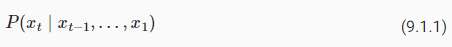
Such models that regress the value of a signal on the previous values of that same signal are naturally called autoregressive models. There is just one major problem: the number of inputs, xt−1,…,x1 varies, depending on t. Namely, the number of inputs increases with the amount of data that we encounter. Thus if we want to treat our historical data as a training set, we are left with the problem that each example has a different number of features. Much of what follows in this chapter will revolve around techniques for overcoming these challenges when engaging in such autoregressive modeling problems where the object of interest is P(xt∣xt−1,…,x1) or some statistic(s) of this distribution.
동일한 신호의 이전 값에서 신호 값을 회귀하는 이러한 모델을 자연스럽게 자동 회귀 모델(autoregressive models)이라고 합니다. 여기에는 하나의 주요 문제가 있습니다. 입력 수 xt−1,…,x1은 t에 따라 다릅니다. 즉, (주가는 계속 변하고 그 변한 모든 값들이 예측에 input으로 사용되기 때문에 input 값들은 계속 증가하게 된다.). 따라서 과거 데이터를 훈련 세트로 취급하려는 경우 각 example 별로 different number of features가 있다는 문제가 남습니다. 이 장에서 이어지는 내용의 대부분은 관심 대상이 P(xt∣xt−1,…,x1) 또는 이 분포의 일부 통계인 autoregressive modeling 문제에 관여할 때 이러한 문제를 극복하기 위한 기술을 중심으로 전개됩니다.
(주가는 계속 변하고 그 변한 모든 값들이 예측에 input으로 사용되기 때문에 input 값들은 계속 증가하게 된다.)
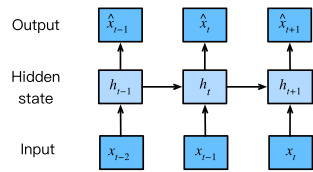
A few strategies recur frequently. First of all, we might believe that although long sequences xt−1,…,x1 are available, it may not be necessary to look back so far in the history when predicting the near future. In this case we might content ourselves to condition on some window of length τ and only use xt−1,…,xt−τ observations. The immediate benefit is that now the number of arguments is always the same, at least for t>τ. This allows us to train any linear model or deep network that requires fixed-length vectors as inputs. Second, we might develop models that maintain some summary ℎt of the past observations (see Fig. 9.1.2) and at the same time update ℎt in addition to the prediction x^t. This leads to models that estimate xt with x^t=P(xt∣ℎt) and moreover updates of the form ℎt=g(ℎt−1,xt−1). Since ℎt is never observed, these models are also called latent autoregressive models.
여기에 대해 몇 가지 전략이 자주 반복됩니다. 우선, 우리는 긴 시퀀스 xt−1,...,x1을 사용할 수 있지만 가까운 미래를 예측할 때 지금까지의 역사를 되돌아볼 필요가 없다고 믿을 수 있습니다. 이 경우 길이 τ의 일부 창에 대한 조건에 만족하고 xt−1,,xt−τ 관측만 사용할 수 있습니다. 즉각적인 이점은 이제 인수(arguments)의 수가 적어도 t>τ에 대해 항상 동일하다는 것입니다. 이를 통해 고정 길이 벡터가 입력으로 필요한 모든 선형 모델 또는 심층 네트워크를 훈련할 수 있습니다. 둘째, 우리는 과거 관찰의 일부 요약 ℎt를 유지하고(그림 9.1.2 참조) 동시에 예측 x^t에 추가하여 ℎt를 업데이트하는 모델을 개발할 수 있습니다. 이로 인해 x^t=P(xt∣ℎt)로 xt를 추정하는 모델과 ℎt=g(ℎt−1,xt−1) 형식의 업데이트가 생성됩니다. ℎt는 관찰되지 않기 때문에 이러한 모델은 잠재 자기회귀 모델(latent autoregressive models)이라고도 합니다.
To construct training data from historical data, one typically creates examples by sampling windows randomly. In general, we do not expect time to stand still. However, we often assume that while the specific values of xt might change, the dynamics according to which each subsequent observation is generated given the previous observations do not. Statisticians call dynamics that do not change stationary.
기록 데이터(historical data)에서 교육 데이터(raining data)를 구성하려면 일반적으로 창을 무작위로 샘플링하여 예제를 만드는 겁니다. 일반적으로 우리는 시간이 멈출 것이라고 기대하지 않습니다. 그러나 우리는 종종 xt의 특정 값이 변경될 수 있지만 이전 관찰이 주어진 경우 각 후속 관찰이 생성되는 역학은 그렇지 않다고 가정합니다. 통계학자들은 그 고정된 상태로 변하지 않는 역학을 찾는 겁니다.
9.1.2. Sequence Models
Sometimes, especially when working with language, we wish to estimate the joint probability of an entire sequence. This is a common task when working with sequences composed of discrete tokens, such as words. Generally, these estimated functions are called sequence models and for natural language data, they are called language models. The field of sequence modeling has been driven so much by natural language processing, that we often describe sequence models as “language models”, even when dealing with non-language data. Language models prove useful for all sorts of reasons. Sometimes we want to evaluate the likelihood of sentences. For example, we might wish to compare the naturalness of two candidate outputs generated by a machine translation system or by a speech recognition system. But language modeling gives us not only the capacity to evaluate likelihood, but the ability to sample sequences, and even to optimize for the most likely sequences.
때때로, 특히 언어로 작업할 때 전체 시퀀스의 결합 확률(joint probability)을 추정하려고 합니다. 이는 단어와 같은 개별 토큰으로 구성된 시퀀스로 작업할 때 일반적인 작업입니다. 일반적으로 이러한 추정 함수를 시퀀스 모델이라고 하고 자연어 데이터의 경우 언어 모델(language models)이라고 합니다. 시퀀스 모델링 분야는 자연어 처리에 의해 많이 구동되어 비언어 데이터를 처리할 때에도 시퀀스 모델을 "언어 모델"로 설명하는 경우가 많습니다. 언어 모델은 여러 가지 이유로 유용합니다. 때때로 우리는 문장의 가능성을 평가하기를 원합니다. 예를 들어 기계 번역 시스템 또는 음성 인식 시스템에서 생성된 두 후보 output 중 어느것이 더 자연스러운지 비교하고자 할 수 있습니다. 언어 모델링은 evaluate likelihood 능력뿐만 아니라 시퀀스를 샘플링하고 가장 가능성이 높은 시퀀스를 최적화할 수 있는 능력도 제공합니다.
While language modeling might not look, at first glance, like an autoregressive problem, we can reduce language modeling to autoregressive prediction by decomposing the joint density of a sequence p(xt∣x1,…,xT) into the product of conditional densities in a left-to-right fashion by applying the chain rule of probability:
언뜻 보기에 언어 모델링이 자동회귀 문제처럼 보이지 않을 수도 있지만 시퀀스 p(xt∣x1,…,xT)의 결합 밀도를 조건부 밀도의 곱으로 분해하여 언어 모델링을 자동회귀 예측으로 줄일 수 있습니다. 확률의 연쇄 법칙을 적용하여 왼쪽에서 오른쪽으로:

Note that if we are working with discrete signals like words, then the autoregressive model must be a probabilistic classifier, outputting a full probability distribution over the vocabulary for what word will come next, given the leftwards context.
단어와 같은 불연속 신호로 작업하는 경우 자동 회귀 모델은 주어진 왼쪽 컨텍스트에서 단어가 다음에 올 것인지에 대한 전체 확률 분포를 어휘에 대해 출력하는 확률적 분류기여야 합니다.
Sequence Model or Language Model 이란?
Sequence models, also known as language models, are a class of statistical models used to predict or generate sequences of data. In the context of natural language processing (NLP), language models specifically focus on predicting or generating sequences of words or tokens in a language. These models are designed to understand the structure and patterns in the sequence of words and capture the dependencies between different words in the text.
시퀀스 모델 또는 언어 모델은 데이터의 시퀀스를 예측하거나 생성하는 데 사용되는 통계적 모델의 한 유형입니다. 자연어 처리(NLP)의 맥락에서 특히 언어 모델은 언어 내 단어 또는 토큰의 시퀀스를 예측하거나 생성하는 데 초점을 맞춥니다. 이러한 모델은 텍스트 내 단어 시퀀스의 구조와 패턴을 이해하고 단어들 사이의 의존성을 파악하는 데 사용됩니다.
Language models are essential in various NLP tasks, such as text generation, machine translation, speech recognition, sentiment analysis, and more. They can be trained on large amounts of text data to learn the probabilities of word sequences and their context in a language. With this knowledge, language models can generate coherent and contextually relevant text, given a starting word or sentence.
언어 모델은 텍스트 생성, 기계 번역, 음성 인식, 감성 분석 등 다양한 NLP 작업에서 중요한 역할을 합니다. 이러한 모델은 대량의 텍스트 데이터를 학습하여 단어 시퀀스와 언어 내 문맥의 확률을 학습합니다. 이러한 지식을 활용하여 언어 모델은 시작 단어나 문장을 기준으로 논리적이고 문맥에 맞는 텍스트를 생성할 수 있습니다.
One of the key components of language models is the ability to consider the context of a word by looking at the preceding words, which is often referred to as autoregressive behavior. This context helps the model make more accurate predictions and generate meaningful text. There are various architectures and techniques used to build language models, including Recurrent Neural Networks (RNNs), Long Short-Term Memory (LSTM) networks, and Transformer-based models like GPT (Generative Pre-trained Transformer).
언어 모델의 중요한 구성 요소 중 하나는 단어의 문맥을 고려하여 이전 단어들을 살펴보는 능력입니다. 이를 자기회귀적 특성이라고도 합니다. 이러한 문맥은 모델이 보다 정확한 예측을 수행하고 의미 있는 텍스트를 생성하는 데 도움을 줍니다. RNN(순환 신경망), LSTM(장단기 메모리) 네트워크, GPT(생성적 사전 훈련 트랜스포머)과 같은 트랜스포머 기반 모델 등 다양한 아키텍처와 기법이 언어 모델 구축에 사용됩니다.
Overall, sequence models or language models play a crucial role in natural language processing and have revolutionized many NLP applications by enabling computers to understand and generate human-like language.
전반적으로 시퀀스 모델 또는 언어 모델은 자연어 처리에 핵심적인 역할을 하며, 컴퓨터가 인간과 유사한 언어를 이해하고 생성할 수 있도록 여러 NLP 응용 프로그램을 혁신적으로 바꾸어 놓았습니다.
9.1.2.1. Markov Models
Now suppose that we wish to employ the strategy mentioned above, where we condition only on the τ previous time steps, i.e., xt−1,…,xt−τ, rather than the entire sequence history xt−1,…,x1. Whenever we can throw away the history beyond the precious τ steps without any loss in predictive power, we say that the sequence satisfies a Markov condition, i.e., that the future is conditionally independent of the past, given the recent history. When τ=1, we say that the data is characterized by a first-order Markov model, and when τ=k, we say that the data is characterized by a k-th order Markov model. For when the first-order Markov condition holds (τ=1) the factorization of our joint probability becomes a product of probabilities of each word given the previous word:
이제 전체 시퀀스 히스토리 xt-1,...,x1이 아니라 τ 이전 시간 단계, 즉 xt-1,...,xt-τ에 대해서만 조건을 지정하는 위에서 언급한 전략을 사용하려고 한다고 가정합니다. 예측력의 손실 없이 귀중한 τ 단계를 넘어선 history를 버릴 수 있을 때마다 우리는 시퀀스가 Markov condition을 충족한다고 말합니다. τ=1이면 데이터가 1차 Markov 모델로 특징지어진다고 하고 τ=k이면 데이터가 k차 Markov 모델로 특징지어진다고 합니다. 1차 Markov 조건이 유지될 때(τ=1) 결합 확률의 분해는 이전 단어가 주어진 각 단어의 product of probabilities이 됩니다.

We often find it useful to work with models that proceed as though a Markov condition were satisfied, even when we know that this is only approximately true. With real text documents we continue to gain information as we include more and more leftwards context. But these gains diminish rapidly. Thus, sometimes we compromise, obviating computational and statistical difficulties by training models whose validity depends on a k-th order Markov condition. Even today’s massive RNN- and Transformer-based language models seldom incorporate more than thousands of words of context.
Markov 조건이 만족된 것처럼 진행되는 모델로 작업하는 것이 유용하다는 것을 종종 알게 됩니다. 이것이 거의 사실이라는 것을 알고 있을 때도 마찬가지입니다. 실제 텍스트 문서를 통해 우리는 점점 더 왼쪽 컨텍스트를 포함함에 따라 정보를 계속 얻습니다. 그러나 이러한 이득은 빠르게 감소합니다. 따라서 때때로 우리는 타당성이 k차 마르코프 조건에 의존하는 훈련 모델을 통해 계산 및 통계적 어려움을 없애 타협합니다. 오늘날의 대규모 RNN 및 Transformer 기반 언어 모델도 수천 단어 이상의 컨텍스트를 통합하는 경우는 거의 없습니다.
With discrete data, a true Markov model simply counts the number of times that each word has occurred in each context, producing the relative frequency estimate of P(xt∣xt−1). Whenever the data assumes only discrete values (as in language), the most likely sequence of words can be computed efficiently using dynamic programming.
불연속 데이터를 사용하는 진정한 Markov 모델은 단순히 각 단어가 각 컨텍스트에서 발생한 횟수를 계산하여 P(xt∣xt−1)의 상대 빈도 추정치(relative frequency estimate)를 생성합니다. 데이터가 이산 값(discrete values)(언어에서와 같이)만 가정할 때마다 동적 프로그래밍을 사용하여 가장 가능성이 높은 단어 시퀀스를 효율적으로 계산할 수 있습니다.
Markov Model 이란?
Markov Models, named after the Russian mathematician Andrey Markov, are a class of probabilistic models that capture the dependencies between a sequence of random events. These models assume that the probability of a future event depends only on the current state and is independent of the history of past events. In other words, they exhibit the Markov property, which states that the future is conditionally independent of the past given the present state.
마르코프 모델은 러시아의 수학자 앤드리 마르코프에 따라 이름 붙여진 확률적 모델의 한 종류로, 일련의 무작위 사건들 간의 의존성을 포착합니다. 이 모델은 미래 사건의 확률이 현재 상태에만 의존하며 과거 사건의 히스토리와는 독립적이라고 가정합니다. 즉, 마르코프 모델은 현재 상태가 주어진다면 미래가 과거에 대해 조건부 독립적이라는 마르코프 속성을 나타냅니다.
Markov Models are widely used in various fields, including natural language processing, speech recognition, finance, and bioinformatics. They have applications in language modeling, part-of-speech tagging, hidden Markov models for speech recognition, and more. The key components of Markov Models are the state space, transition probabilities, and initial state probabilities, which define how the model moves from one state to another.
마르코프 모델은 자연어 처리, 음성 인식, 금융, 생물 정보학 등 다양한 분야에서 널리 사용됩니다. 이들은 언어 모델링, 품사 태깅, 음성 인식을 위한 숨겨진 마르코프 모델 등에 적용됩니다. 마르코프 모델의 주요 구성 요소는 상태 공간, 전이 확률 및 초기 상태 확률이며, 이들은 모델이 한 상태에서 다른 상태로 이동하는 방식을 정의합니다.
9.1.2.2. The Order of Decoding
You might be wondering, why did we have to represent the factorization of a text sequence P(x1,…,xT) as a left-to-right chain of conditional probabilities. Why not right-to-left or some other, seemingly random order? In principle, there is nothing wrong with unfolding P(x1,…,xT) in reverse order. The result is a valid factorization:
텍스트 시퀀스 P(x1,…,xT)의 분해를 조건부 확률(conditional probabilities)의 왼쪽에서 오른쪽 체인으로 표현해야 하는 이유가 궁금할 수 있습니다. 오른쪽에서 왼쪽으로 또는 다른 무작위 순서로 표시되지 않는 이유는 무엇입니까? 원칙적으로 P(x1,…,xT)를 역순으로 펼치는 것은 잘못된 것이 아닙니다. 결과는 유효한 인수분해입니다.

However, there are many reasons why factorizing text in the same directions as we read it (left-to-right for most languages, but right-to-left for Arabic and Hebrew) is preferred for the task of language modeling. First, this is just a more natural direction for us to think about. After all we all read text every day, and this process is guided by our ability to anticipate what words and phrases are likely to come next. Just think of how many times you have completed someone else’s sentence. Thus, even if we had no other reason to prefer such in-order decodings, they would be useful if only because we have better intuitions for what should be likely when predicting in this order.
그러나 우리가 읽는 것과 같은 방향(대부분의 언어에서는 왼쪽에서 오른쪽으로, 아랍어와 히브리어에서는 오른쪽에서 왼쪽으로)으로 텍스트를 분해하는 것이 언어 모델링 작업에 선호되는 데는 여러 가지 이유가 있습니다. 첫째, 이것은 우리가 생각하기에 더 자연스러운 방향일 뿐입니다. 결국 우리 모두는 매일 텍스트를 읽고 이 프로세스는 다음에 올 단어와 구문을 예상하는 능력에 따라 결정됩니다. 다른 사람의 문장을 몇 번이나 완성했는지 생각해 보십시오. 따라서 우리가 이러한 순차 디코딩을 선호할 다른 이유가 없더라도 이 순서로 예측할 때 발생할 수 있는 일에 대해 더 나은 직관을 가지고 있기 때문에 유용할 것입니다.
Second, by factorizing in order, we can assign probabilities to arbitrarily long sequences using the same language model. To convert a probability over steps 1 through t into one that extends to word t+1 we simply multiply by the conditional probability of the additional token given the previous ones: P(xt+1,…,x1)=P(xt,…,x1)⋅P(xt+1∣xt,…,x1).
둘째, 순서대로 분해함으로써 동일한 언어 모델을 사용하여 임의의 긴 시퀀스에 확률을 할당할 수 있습니다. 1단계에서 t단계까지의 확률을 단어 t+1로 확장되는 확률로 변환하려면 이전 토큰에 주어진 추가 토큰의 조건부 확률을 곱하기만 하면 됩니다. P(xt+1,…,x1)=P(xt,… ,x1)⋅P(xt+1∣xt,…,x1).
Third, we have stronger predictive models for predicting adjacent words versus words at arbitrary other locations. While all orders of factorization are valid, they do not necessarily all represent equally easy predictive modeling problems. This is true not only for language, but for other kinds of data as well, e.g., when the data is causally structured. For example, we believe that future events cannot influence the past. Hence, if we change xt, we may be able to influence what happens for xt+1 going forward but not the converse. That is, if we change xt, the distribution over past events will not change. In some contexts, this makes it easier to predict P(xt+1∣xt) than to predict P(xt∣xt+1). For instance, in some cases, we can find xt+1=f(xt)+ϵ for some additive noise ϵ, whereas the converse is not true (Hoyer et al., 2009). This is great news, since it is typically the forward direction that we are interested in estimating. The book by Peters et al. (2017) has explained more on this topic. We are barely scratching the surface of it.
셋째, 임의의 다른 위치에 있는 단어에 비해 인접 단어를 예측하기 위한 더 강력한 예측 모델이 있습니다. 모든 분해 순서가 유효하지만 모두 똑같이 쉬운 예측 모델링 문제를 나타내는 것은 아닙니다. 이것은 언어뿐만 아니라 다른 종류의 데이터(예: 데이터가 인과적으로 구조화된 경우)에도 해당됩니다. 예를 들어, 우리는 미래의 사건이 과거에 영향을 미칠 수 없다고 믿습니다. 따라서 xt를 변경하면 앞으로 xt+1에 대해 어떤 일이 발생하는지에 영향을 미칠 수 있지만 그 반대의 경우에는 영향을 미치지 않습니다. 즉, xt를 변경하면 과거 이벤트에 대한 분포가 변경되지 않습니다. 어떤 상황에서는 P(xt∣xt+1)를 예측하는 것보다 P(xt+1∣xt)를 예측하는 것이 더 쉽습니다. 예를 들어 어떤 경우에는 일부 추가 노이즈 ϵ에 대해 xt+1=f(xt)+ϵ를 찾을 수 있지만 그 반대는 사실이 아닙니다(Hoyer et al., 2009). 이것은 일반적으로 우리가 추정하는 데 관심이 있는 전방 방향이기 때문에 좋은 소식입니다. Peters et al(2017)의 저서에서 이 주제에 대해 자세히 설명했습니다. 우리는 그것의 표면을 간신히 긁고 있습니다.
9.1.3. Training
Before we focus our attention on text data, let’s first try this out with some continuous-valued synthetic data.
텍스트 데이터에 집중하기 전에 먼저 연속 값 합성 데이터로 시도해 보겠습니다.
Here, our 1000 synthetic data will follow the trigonometric sin function, applied to 0.01 times the time step. To make the problem a little more interesting, we corrupt each sample with additive noise. From this sequence we extract training examples, each consisting of features and a label.
여기에서 1000개의 합성 데이터는 시간 단계의 0.01배에 적용된 삼각 함수(trigonometric sin function)를 따릅니다. 문제를 좀 더 흥미롭게 만들기 위해 추가 노이즈로 각 샘플을 손상시킵니다. 이 시퀀스에서 각각 기능과 레이블로 구성된 훈련 예제를 추출합니다.
class Data(d2l.DataModule):
    def __init__(self, batch_size=16, T=1000, num_train=600, tau=4):
        self.save_hyperparameters()
        self.time = torch.arange(1, T + 1, dtype=torch.float32)
        self.x = torch.sin(0.01 * self.time) + torch.randn(T) * 0.2

data = Data()
d2l.plot(data.time, data.x, 'time', 'x', xlim=[1, 1000], figsize=(6, 3))
위 코드는 Data라는 클래스를 정의하는 코드입니다. Data 클래스는 d2l.DataModule을 상속하여 만들어졌습니다. 클래스 내부에서는 다양한 매개변수들을 설정하고, 시계열 데이터를 생성하는 로직이 포함되어 있습니다.
Data 클래스의 생성자(__init__)에서는 다음과 같은 매개변수들을 받습니다:
- batch_size: 배치 크기를 지정하는 매개변수로, 기본값은 16입니다.
- T: 시계열 데이터의 길이를 지정하는 매개변수로, 기본값은 1000입니다.
- num_train: 훈련 데이터의 개수를 지정하는 매개변수로, 기본값은 600입니다.
- tau: 생성된 시계열 데이터에 노이즈를 추가할 때 사용되는 시간 스케일을 지정하는 매개변수로, 기본값은 4입니다.
Data 클래스의 주요 기능은 time과 x라는 두 개의 텐서를 생성하는 것입니다. time 텐서는 1부터 T까지의 시간값을 포함하고 있으며, x 텐서는 이 시간값에 대한 사인 함수와 노이즈를 추가한 결과를 저장합니다.
마지막으로 d2l.plot 함수를 사용하여 시계열 데이터를 그래프로 표시합니다. data.time은 시간값을, data.x는 해당 시간값에 대한 신호값을 나타냅니다. 그래프는 time을 x축으로, x를 y축으로하여 그려집니다. xlim=[1, 1000]은 x축의 범위를 1부터 1000까지로 지정하며, figsize=(6, 3)은 그래프의 크기를 지정합니다.


To begin, we try a model that acts as though the data satisfied a τ-order Markov condition, and thus predicts xt using only the past τ observations. Thus for each time step we have an example with label y=xt and features xt=[xt−τ,…,xt−1]. The astute reader might have noticed that this results in 1000−τ examples, since we lack sufficient history for y1,…,yτ. While we could pad the first τ sequences with zeros, to keep things simple, we drop them for now. The resulting dataset contains T−τ examples, where each input to the model has sequence length τ. We create a data iterator on the first 600 examples, covering a period of the sin function.
시작하려면 데이터가 τ-order Markov 조건을 충족하는 것처럼 작동하는 모델을 시도하여 과거 τ 관측값만 사용하여 xt를 예측합니다. 따라서 각 시간 단계에 대해 레이블 y=xt 및 feature xt=[xt−τ,…,xt−1]이 있는 예가 있습니다. 기민한 독자라면 y1,...,yτ에 대한 충분한 이력이 부족하기 때문에 이것이 1000−τ 예가 된다는 것을 알아차렸을 것입니다. 첫 번째 τ 시퀀스를 0으로 채울 수 있지만 간단하게 유지하기 위해 지금은 삭제합니다. 결과 데이터 세트에는 모델에 대한 각 입력의 시퀀스 길이 τ가 있는 T−τ 예제가 포함됩니다. sin 함수의 기간을 포함하는 처음 600개의 예제에 대한 데이터 반복자를 만듭니다.
@d2l.add_to_class(Data)
def get_dataloader(self, train):
    features = [self.x[i : self.T-self.tau+i] for i in range(self.tau)]
    self.features = torch.stack(features, 1)
    self.labels = self.x[self.tau:].reshape((-1, 1))
    i = slice(0, self.num_train) if train else slice(self.num_train, None)
    return self.get_tensorloader([self.features, self.labels], train, i)
위 코드는 Data 클래스에 새로운 메서드인 get_dataloader를 추가하는 코드입니다. 이 메서드는 데이터로더를 생성하여 반환하는 역할을 합니다.
get_dataloader 메서드는 다음과 같은 인자들을 받습니다:
- self: 현재 클래스 객체를 나타내는 매개변수입니다.
- train: 데이터 로더를 훈련용으로 생성할지 테스트용으로 생성할지를 결정하는 불리언 매개변수입니다.
이 메서드의 주요 기능은 다음과 같습니다:
- 시계열 데이터 self.x를 입력으로 받아서, self.tau 값에 따라 시계열 데이터를 tau 길이의 텐서 슬라이딩 윈도우로 분할합니다. 분할된 각 시계열 데이터는 특성으로 사용될 것입니다.
- 생성된 특성(features)과 레이블(labels) 데이터를 각각 torch.stack을 사용하여 텐서로 변환합니다.
- 훈련용 데이터와 테스트용 데이터를 구분하여 데이터 로더를 생성하고 반환합니다.
구체적으로, features는 길이가 tau인 시계열 데이터의 슬라이딩 윈도우로, labels는 시계열 데이터의 tau 이후 값들을 나타냅니다. 훈련용 데이터는 0부터 num_train까지의 범위로, 테스트용 데이터는 num_train부터 끝까지로 나누어집니다.
즉, get_dataloader 메서드는 시계열 데이터를 특성과 레이블로 분할하고, 이를 기반으로 훈련용과 테스트용 데이터 로더를 생성하여 반환합니다.
In this example our model will be a standard linear regression.
이 예에서 모델은 표준 선형 회귀입니다.
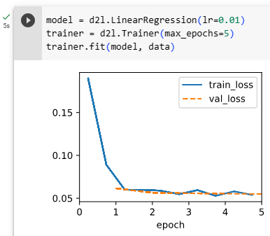
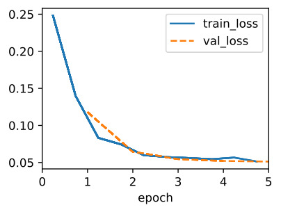
model = d2l.LinearRegression(lr=0.01)
trainer = d2l.Trainer(max_epochs=5)
trainer.fit(model, data)
위 코드는 선형 회귀 모델을 정의하고, 이를 훈련하는 코드입니다.
- d2l.LinearRegression(lr=0.01): d2l 라이브러리의 LinearRegression 클래스를 사용하여 선형 회귀 모델을 정의합니다. 이 모델은 입력과 가중치를 곱하고 편향을 더한 선형 연산을 수행하는 간단한 선형 모델입니다. lr=0.01은 학습률(learning rate)을 나타내며, 경사 하강법(gradient descent)에서 가중치 업데이트 시 사용되는 스케일링 비율을 의미합니다.
- trainer = d2l.Trainer(max_epochs=5): d2l 라이브러리의 Trainer 클래스를 사용하여 훈련을 관리하는 객체 trainer를 생성합니다. max_epochs=5는 최대 에포크(epoch) 수를 의미하며, 훈련 데이터를 5회 반복하여 모델을 업데이트하는 것을 의미합니다.
- trainer.fit(model, data): trainer 객체를 사용하여 정의된 선형 회귀 모델(model)을 주어진 데이터(data)에 대해 훈련합니다. 이를 위해 경사 하강법 알고리즘을 사용하여 모델의 가중치를 조정하고, 주어진 훈련 데이터를 활용하여 모델을 훈련합니다.
즉, 위 코드는 주어진 데이터를 활용하여 선형 회귀 모델을 훈련하는 과정을 나타냅니다.
9.1.4. Prediction
To evaluate our model, we first check how well our model performs at one-step-ahead prediction.
모델을 평가하기 위해 먼저 모델이 one-step-ahead prediction에서 얼마나 잘 수행되는지 확인합니다.
onestep_preds = model(data.features).detach().numpy()
d2l.plot(data.time[data.tau:], [data.labels, onestep_preds], 'time', 'x',
         legend=['labels', '1-step preds'], figsize=(6, 3))
위 코드는 훈련된 선형 회귀 모델을 사용하여 1단계 예측을 수행하고, 이를 시각화하는 과정을 나타냅니다.
- onestep_preds = model(data.features).detach().numpy(): 훈련된 선형 회귀 모델(model)을 주어진 입력 데이터 data.features에 적용하여 1단계 예측값(onestep_preds)을 얻습니다. detach() 함수는 연산 그래프로부터 분리하여 예측값을 얻고, numpy() 함수는 PyTorch 텐서를 NumPy 배열로 변환합니다.
- d2l.plot(data.time[data.tau:], [data.labels, onestep_preds], 'time', 'x', legend=['labels', '1-step preds'], figsize=(6, 3)): d2l 라이브러리의 plot 함수를 사용하여 시간(time)에 따른 실제 레이블(data.labels)과 1단계 예측값(onestep_preds)을 시각화합니다. data.time[data.tau:]은 입력 데이터의 시간을 뜻하며, legend 인자를 사용하여 범례를 설정합니다. figsize는 그림의 크기를 지정하는 인자입니다.
즉, 위 코드는 훈련된 선형 회귀 모델을 이용하여 시간에 따른 데이터에 대해 1단계 예측을 수행하고, 이를 실제 레이블과 함께 그래프로 시각화하는 과정을 나타냅니다.

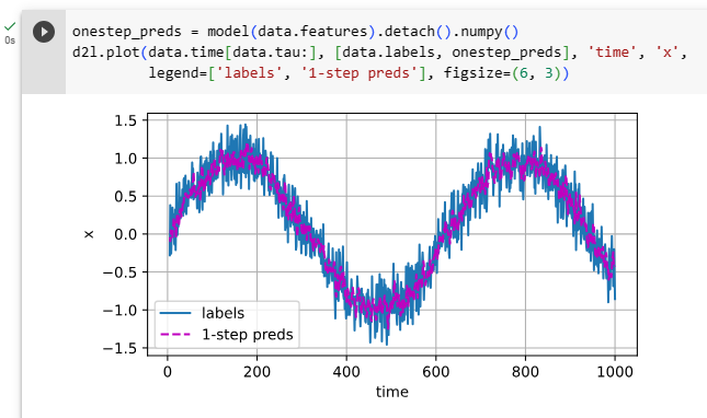
The one-step-ahead predictions look good, even near the end t=1000.
one-step-ahead predictions은 t=1000의 끝 근처에서도 좋아 보입니다.
Now consider, what if we only observed sequence data up until time step 604 (n_train + tau) but wished to make predictions several steps into the future. Unfortunately, we cannot directly compute the one-step-ahead prediction for time step 609, because we do not know the corresponding inputs, having seen only up to x604. We can address this problem by plugging in our earlier predictions as inputs to our model for making subsequent predictions, projecting forward, one step at a time, until reaching the desired time step:
이제 우리가 시간 단계 604(n_train + tau)까지만 시퀀스 데이터를 관찰했지만 미래의 여러 단계를 예측하고자 한다면 어떻게 될까요? 불행히도 x604까지만 보았기 때문에 해당 입력을 모르기 때문에 시간 단계 609에 대한 한 단계 앞선 예측을 직접 계산할 수 없습니다. 원하는 시간 단계에 도달할 때까지 한 번에 한 단계 앞으로 예측하여 후속 예측을 하기 위한 모델에 대한 입력으로 이전 예측을 연결하여 이 문제를 해결할 수 있습니다.

Generally, for an observed sequence x1,…,xt, its predicted output x^t+k at time step t+k is called the k-step-ahead prediction. Since we have observed up to x604, its k-step-ahead prediction is x^604+k. In other words, we will have to keep on using our own predictions to make multistep-ahead predictions. Let’s see how well this goes.
일반적으로 관찰된 시퀀스 x1,...,xt의 경우 시간 단계 t+k에서 예측된 출력 x^t+k를 k-step-ahead 예측이라고 합니다. x604까지 관찰했기 때문에 k-step-ahead 예측은 x^604+k입니다. 다시 말해, 우리는 다단계 예측을 하기 위해 우리 자신의 예측을 계속 사용해야 할 것입니다. 이것이 얼마나 잘되는지 봅시다.
multistep_preds = torch.zeros(data.T)
multistep_preds[:] = data.x
for i in range(data.num_train + data.tau, data.T):
    multistep_preds[i] = model(
        multistep_preds[i - data.tau:i].reshape((1, -1)))
multistep_preds = multistep_preds.detach().numpy()

d2l.plot([data.time[data.tau:], data.time[data.num_train+data.tau:]],
         [onestep_preds, multistep_preds[data.num_train+data.tau:]], 'time',
         'x', legend=['1-step preds', 'multistep preds'], figsize=(6, 3))
위 코드는 훈련된 선형 회귀 모델을 사용하여 다중 단계 예측을 수행하고, 이를 시각화하는 과정을 나타냅니다.
- multistep_preds = torch.zeros(data.T): 다중 단계 예측 값을 저장할 텐서 multistep_preds를 생성하고, 모든 값을 0으로 초기화합니다. 이 텐서는 모델을 사용하여 예측한 결과를 저장하는 용도로 사용됩니다.
- multistep_preds[:] = data.x: multistep_preds의 첫 부분은 입력 데이터의 첫 부분(data.x)과 동일하게 초기화합니다.
- for i in range(data.num_train + data.tau, data.T):: 훈련 데이터 이후부터 시작하여 data.T까지 반복하며 다중 단계 예측을 수행합니다.
- multistep_preds[i] = model(multistep_preds[i - data.tau:i].reshape((1, -1))): i 시점 이전의 값을 입력으로 사용하여 모델(model)을 통해 i 시점의 다중 단계 예측값을 얻습니다. reshape 함수를 사용하여 입력 데이터의 차원을 조정합니다.
- multistep_preds = multistep_preds.detach().numpy(): 최종적으로 다중 단계 예측 결과를 PyTorch 텐서에서 NumPy 배열로 변환합니다.
- d2l.plot([data.time[data.tau:], data.time[data.num_train+data.tau:]], [onestep_preds, multistep_preds[data.num_train+data.tau:]], 'time', 'x', legend=['1-step preds', 'multistep preds'], figsize=(6, 3)): d2l 라이브러리의 plot 함수를 사용하여 시간(time)에 따른 1단계 예측값과 다중 단계 예측값을 시각화합니다. data.time[data.tau:]은 입력 데이터의 시간을 뜻하며, legend 인자를 사용하여 범례를 설정합니다. figsize는 그림의 크기를 지정하는 인자입니다.
즉, 위 코드는 훈련된 선형 회귀 모델을 이용하여 다중 단계 예측을 수행하고, 이를 시간에 따라 그래프로 시각화하는 과정을 나타냅니다. 다중 단계 예측은 훈련 데이터 이후의 값을 이용하여 미래 시점의 값을 예측하는 방식으로 이루어집니다.
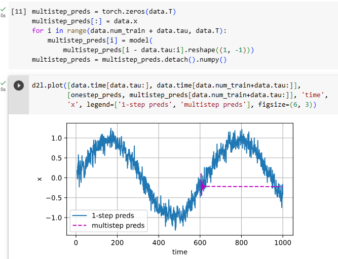
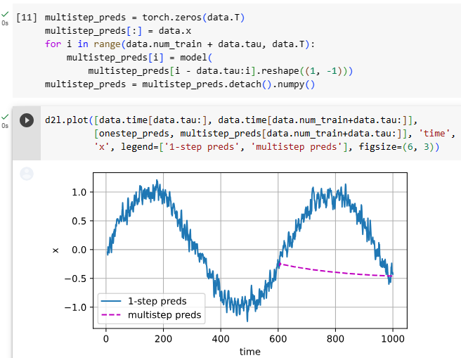

Unfortunately, in this case we fail spectacularly. The predictions decay to a constant pretty quickly after a few prediction steps. Why did the algorithm perform so much worse when predicting further into the future? Ultimately, this owes to the fact that errors build up. Let’s say that after step 1 we have some error ϵ1=ϵ¯. Now the input for step 2 is perturbed by ϵ1, hence we suffer some error in the order of ϵ2=ϵ¯+cϵ1 for some constant c, and so on. The predictions can diverge rapidly from the true observations. You may already be familiar with this common phenomenon. For instance, weather forecasts for the next 24 hours tend to be pretty accurate but beyond that, accuracy declines rapidly. We will discuss methods for improving this throughout this chapter and beyond.
불행하게도 이 경우 우리는 극적으로 실패합니다. 예측은 몇 가지 예측 단계 후에 매우 빠르게 상수로 감소합니다. 더 먼 미래를 예측할 때 알고리즘의 성능이 훨씬 더 나빠진 이유는 무엇입니까? 궁극적으로 이것은 오류가 누적된다는 사실에 기인합니다. 1단계 이후에 오류 ϵ1=ϵ¯가 발생했다고 가정해 보겠습니다. 이제 2단계의 입력은 ϵ1에 의해 교란되므로 일부 상수 c에 대해 ϵ2=ϵ+cϵ1의 순서로 약간의 오류가 발생합니다. 예측은 실제 관찰과 빠르게 다를 수 있습니다. 이 일반적인 현상에 이미 익숙할 수 있습니다. 예를 들어, 다음 24시간 동안의 일기 예보는 꽤 정확한 경향이 있지만 그 이상으로 정확도가 급격히 떨어집니다. 이 장과 그 이후에 이를 개선하는 방법에 대해 논의할 것입니다.
Let’s take a closer look at the difficulties in k-step-ahead predictions by computing predictions on the entire sequence for k=1,4,16,64.
k=1,4,16,64에 대한 전체 시퀀스에 대한 예측을 계산하여 k-step-ahead 예측의 어려움을 자세히 살펴보겠습니다.
def k_step_pred(k):
    features = []
    for i in range(data.tau):
        features.append(data.x[i : i+data.T-data.tau-k+1])
    # The (i+tau)-th element stores the (i+1)-step-ahead predictions
    for i in range(k):
        preds = model(torch.stack(features[i : i+data.tau], 1))
        features.append(preds.reshape(-1))
    return features[data.tau:]

steps = (1, 4, 16, 64)
preds = k_step_pred(steps[-1])
d2l.plot(data.time[data.tau+steps[-1]-1:],
         [preds[k - 1].detach().numpy() for k in steps], 'time', 'x',
         legend=[f'{k}-step preds' for k in steps], figsize=(6, 3))
위 코드는 k_step_pred라는 함수를 정의하고, 이를 사용하여 다양한 단계의 다음 예측값을 계산하고 시각화하는 과정을 나타냅니다.
- def k_step_pred(k):: k_step_pred라는 함수를 정의합니다. 이 함수는 인자 k를 받아 다음 k 단계의 예측값을 계산합니다.
- for i in range(data.tau):: data.tau까지 반복하며 features라는 리스트에 입력 데이터의 부분 시퀀스를 추가합니다. 이를 통해 다음 예측을 위한 입력 데이터를 구성합니다.
- for i in range(k):: k 값 만큼 반복하며 다음 예측값을 계산합니다.
- preds = model(torch.stack(features[i : i+data.tau], 1)): 모델(model)을 사용하여 다음 k 단계의 예측값(preds)을 계산합니다. 입력 데이터는 features 리스트의 부분 시퀀스를 사용하여 구성되며, torch.stack 함수를 사용하여 데이터를 적절히 변형합니다.
- features.append(preds.reshape(-1)): 계산한 다음 예측값을 features 리스트에 추가합니다. 이를 통해 다음 예측에 필요한 입력 데이터를 구성합니다.
- return features[data.tau:]: 예측값을 담고 있는 features 리스트를 data.tau 이후의 값들만 반환합니다. 이는 처음 data.tau 개의 입력 데이터가 예측에 사용되었기 때문에 처음 data.tau 개의 예측값은 제외하고 반환하는 것입니다.
- steps = (1, 4, 16, 64): 다음 예측에 사용할 단계들을 정의합니다. steps에는 1, 4, 16, 64가 저장되어 있습니다.
- preds = k_step_pred(steps[-1]): k_step_pred 함수를 사용하여 64단계 다음의 예측값들을 계산하고, preds에 저장합니다.
- d2l.plot(data.time[data.tau+steps[-1]-1:], [preds[k - 1].detach().numpy() for k in steps], 'time', 'x', legend=[f'{k}-step preds' for k in steps], figsize=(6, 3)): d2l 라이브러리의 plot 함수를 사용하여 시간(time)에 따른 1, 4, 16, 64 단계 다음의 예측값들을 시각화합니다. 각 단계에 해당하는 예측값은 preds에서 가져오며, legend 인자를 사용하여 범례를 설정합니다. figsize는 그림의 크기를 지정하는 인자입니다.
즉, 위 코드는 다음 k 단계의 예측값들을 계산하고 이를 시간에 따라 그래프로 시각화하는 과정을 나타냅니다. k_step_pred 함수는 입력 데이터를 이용하여 다음 k 단계의 예측값을 계산하며, d2l.plot 함수를 사용하여 시각화를 수행합니다. 예측값들은 각각 1, 4, 16, 64 단계 뒤의 값을 예측하는 것으로 구성되어 있습니다.


This clearly illustrates how the quality of the prediction changes as we try to predict further into the future. While the 4-step-ahead predictions still look good, anything beyond that is almost useless.
이것은 우리가 더 먼 미래를 예측하려고 할 때 예측의 품질이 어떻게 변하는지를 명확하게 보여줍니다. 4단계 예측은 여전히 좋아 보이지만 그 이상은 거의 쓸모가 없습니다.
9.1.5. Summary
There is quite a difference in difficulty between interpolation and extrapolation. Consequently, if you have a sequence, always respect the temporal order of the data when training, i.e., never train on future data. Given this kind of data, sequence models require specialized statistical tools for estimation. Two popular choices are autoregressive models and latent-variable autoregressive models. For causal models (e.g., time going forward), estimating the forward direction is typically a lot easier than the reverse direction. For an observed sequence up to time step t, its predicted output at time step t+k is the k-step-ahead prediction. As we predict further in time by increasing k, the errors accumulate and the quality of the prediction degrades, often dramatically.
보간(interpolation,삽입,내삽 )과 외삽(extrapolation,외삽,추정,연장) 사이에는 난이도에 상당한 차이가 있습니다. 결과적으로 시퀀스가 있는 경우 훈련할 때 항상 데이터의 시간적 순서(temporal order)를 존중하십시오. 즉, 미래 데이터에 대해 훈련하지 마십시오. 이러한 종류의 데이터가 주어지면 시퀀스 모델에는 추정을 위한 특수한 통계 도구가 필요합니다. 인기 있는 두 가지 선택은 자동회귀 모델과 잠재 변수 자동회귀 모델입니다. 인과 관계 모델-causal models-(예: 시간 진행)의 경우 일반적으로 정방향을 추정하는 것이 역방향보다 훨씬 쉽습니다. 시간 단계 t까지 관찰된 시퀀스의 경우 시간 단계 t+k에서 예측된 출력은 k-step-ahead 예측입니다. k를 증가시켜 더 많은 시간을 예측하면 오류가 누적되고 예측 품질이 종종 급격하게 저하됩니다.
latent-variable autoregressive models 란?
Latent-variable autoregressive models are a class of probabilistic models that combine autoregressive modeling with the inclusion of latent (hidden) variables. Autoregressive models are a type of sequence model where each element in the sequence is predicted based on the previous elements. In the context of time series data, autoregressive models predict future values based on past observations.
잠재 변수 자기회귀 모델은 자기회귀 모델에 잠재 (숨겨진) 변수를 포함시킨 확률 모델의 한 종류입니다. 자기회귀 모델은 각 시퀀스 요소가 이전 요소들을 기반으로 예측되는 시퀀스 모델의 한 유형입니다. 시계열 데이터의 경우, 자기회귀 모델은 과거 관측치를 기반으로 미래 값을 예측합니다.
In latent-variable autoregressive models, the key idea is to introduce latent variables that capture hidden or unobservable factors that influence the observed data. These latent variables are used to model dependencies and capture complex patterns in the data that cannot be fully explained by the observed variables alone.
잠재 변수 자기회귀 모델에서 중요한 아이디어는 관찰 가능한 데이터만으로 완전히 설명할 수 없는 복잡한 패턴을 포착하는 데 사용되는 숨겨진 변수를 도입하는 것입니다. 이러한 잠재 변수는 데이터의 의존성을 모델링하고, 관찰 변수만으로 설명할 수 없는 복잡한 패턴을 포착하는 데 사용됩니다.
The incorporation of latent variables in autoregressive models enables them to handle more complicated and structured data patterns. These models are widely used in various applications such as natural language processing, speech recognition, finance, and other time series analysis tasks, where the underlying data dependencies may not be directly observable but can be inferred through the latent variables.
잠재 변수가 포함된 자기회귀 모델을 사용하면 더 복잡하고 구조화된 데이터 패턴을 다룰 수 있습니다. 이러한 모델은 자연어 처리, 음성 인식, 금융 및 기타 시계열 분석 작업과 같은 다양한 응용 분야에서 널리 사용됩니다. 이러한 응용 분야에서는 관찰할 수 없는 데이터 의존성을 잠재 변수를 통해 추론할 수 있습니다.
Latent-variable autoregressive models often involve probabilistic inference, where the goal is to learn the distribution of the latent variables conditioned on the observed data. This allows the models to not only make predictions but also estimate uncertainty in their predictions, which is crucial in many real-world scenarios.
잠재 변수 자기회귀 모델은 확률적 추론을 포함하며, 목표는 관찰 데이터에 조건을 걸고 잠재 변수의 분포를 학습하는 것입니다. 이렇게 함으로써 모델은 예측뿐만 아니라 예측의 불확실성을 추정하는 데에도 사용됩니다. 이는 많은 실제 상황에서 중요합니다.
In summary, latent-variable autoregressive models are a powerful class of models that combine autoregressive modeling with the introduction of hidden variables to capture complex dependencies and provide a probabilistic framework for making predictions and handling uncertainty.
요약하면, 잠재 변수 자기회귀 모델은 자기회귀 모델을 확장하여 복잡한 의존성을 포착하고 예측을 수행하며 불확실성을 다루기 위한 확률적 프레임워크를 제공하는 강력한 모델의 한 유형입니다.
9.1.6. Exercises
- Improve the model in the experiment of this section.
- Incorporate more than the past 4 observations? How many do you really need?
- How many past observations would you need if there was no noise? Hint: you can write sin and cos as a differential equation.
- Can you incorporate older observations while keeping the total number of features constant? Does this improve accuracy? Why?
- Change the neural network architecture and evaluate the performance. You may train the new model with more epochs. What do you observe?
- An investor wants to find a good security to buy. He looks at past returns to decide which one is likely to do well. What could possibly go wrong with this strategy?
- Does causality also apply to text? To which extent?
- Give an example for when a latent autoregressive model might be needed to capture the dynamic of the data.
'Dive into Deep Learning > D2L Recurrent Neural Networks (RNN)' 카테고리의 다른 글
| D2L - 9.7. Backpropagation Through Time (0) | 2023.08.02 |
|---|---|
| D2L - 9.6. Concise Implementation of Recurrent Neural Networks (0) | 2023.08.02 |
| D2L - 9.5. Recurrent Neural Network Implementation from Scratch (0) | 2023.08.02 |
| D2L - 9.4. Recurrent Neural Networks (0) | 2023.08.02 |
| D2L - 9.3. Language Models (0) | 2023.08.02 |
| D2L - 9.2. Converting Raw Text into Sequence Data (0) | 2023.08.01 |
| D2L - 9. Recurrent Neural Networks (0) | 2023.07.31 |