

https://d2l.ai/chapter_recurrent-neural-networks/rnn-scratch.html
9.5. Recurrent Neural Network Implementation from Scratch — Dive into Deep Learning 1.0.0-beta0 documentation
d2l.ai
9.5. Recurrent Neural Network Implementation from Scratch
We are now ready to implement an RNN from scratch. In particular, we will train this RNN to function as a character-level language model (see Section 9.4) and train it on a corpus consisting of the entire text of H. G. Wells’ The Time Machine, following the data processing steps outlined in Section 9.2. We start by loading the dataset.
이제 처음부터 RNN을 구현할 준비가 되었습니다. 특히, 우리는 이 RNN이 문자 수준 언어 모델(섹션 9.4 참조)로 기능하도록 훈련하고 H. G. Wells의 The Time Machine의 전체 텍스트로 구성된 코퍼스에서 섹션 9.2에 설명된 데이터 처리 단계에 따라 훈련할 것입니다. . 데이터 세트를 로드하는 것으로 시작합니다.
%matplotlib inline
import math
import torch
from torch import nn
from torch.nn import functional as F
from d2l import torch as d2l
9.5.1. RNN Model
We begin by defining a class to implement the RNN model (Section 9.4.2). Note that the number of hidden units num_hiddens is a tunable hyperparameter.
RNN 모델을 구현하기 위한 클래스를 정의하는 것으로 시작합니다(섹션 9.4.2). 은닉 유닛의 수 num_hiddens는 조정 가능한 하이퍼파라미터입니다.
class RNNScratch(d2l.Module):  #@save
    """The RNN model implemented from scratch."""
    def __init__(self, num_inputs, num_hiddens, sigma=0.01):
        super().__init__()
        self.save_hyperparameters()
        self.W_xh = nn.Parameter(
            torch.randn(num_inputs, num_hiddens) * sigma)
        self.W_hh = nn.Parameter(
            torch.randn(num_hiddens, num_hiddens) * sigma)
        self.b_h = nn.Parameter(torch.zeros(num_hiddens))
위 코드는 PyTorch를 사용하여 구현된 간단한 RNN 모델을 나타냅니다. 이 코드는 스크래치에서 RNN을 구축하는 방법을 보여줍니다.
RNNScratch 클래스는 d2l.Module 클래스를 상속하여 정의되었습니다. 이 클래스는 RNN 모델의 구조와 가중치를 정의합니다.
- __init__ 메서드: RNN 모델의 초기화를 담당합니다. 모델의 하이퍼파라미터(num_inputs, num_hiddens, sigma)를 저장하고, 입력과 숨겨진 상태 사이의 가중치 행렬 W_xh와 숨겨진 상태 간의 가중치 행렬 W_hh, 그리고 숨겨진 상태의 편향 b_h를 정의합니다. 이때 가중치 행렬과 편향은 무작위로 초기화되며, 초기화 값에는 sigma를 곱하여 스케일링합니다.
이렇게 정의된 RNNScratch 클래스는 스크래치에서 구현된 간단한 RNN 모델을 나타내며, 이 모델은 입력과 이전 숨겨진 상태를 활용하여 새로운 숨겨진 상태를 계산하는 역할을 합니다.
The forward method below defines how to compute the output and hidden state at any time step, given the current input and the state of the model at the previous time step. Note that the RNN model loops through the outermost dimension of inputs, updating the hidden state one time step at a time. The model here uses a tanh activation function (Section 5.1.2.3).
아래의 전달 방법은 현재 입력과 이전 시간 단계에서 모델의 상태가 주어지면 임의의 시간 단계에서 출력 및 숨겨진 상태를 계산하는 방법을 정의합니다. RNN 모델은 한 번에 한 단계씩 숨겨진 상태를 업데이트하면서 입력의 가장 바깥쪽 차원을 반복합니다. 여기서 모델은 tanh 활성화 기능을 사용합니다(섹션 5.1.2.3).
@d2l.add_to_class(RNNScratch)  #@save
def forward(self, inputs, state=None):
    if state is None:
        # Initial state with shape: (batch_size, num_hiddens)
        state = torch.zeros((inputs.shape[1], self.num_hiddens),
                          device=inputs.device)
    else:
        state, = state
    outputs = []
    for X in inputs:  # Shape of inputs: (num_steps, batch_size, num_inputs)
        state = torch.tanh(torch.matmul(X, self.W_xh) +
                         torch.matmul(state, self.W_hh) + self.b_h)
        outputs.append(state)
    return outputs, state
위 코드는 앞서 정의한 RNNScratch 클래스에 forward 메서드를 추가하는 부분입니다. 이 메서드는 RNN 모델의 순전파(forward pass) 연산을 정의합니다.
- forward 메서드: RNN 모델의 순전파 연산을 정의합니다. 이 메서드는 두 개의 입력을 받습니다. 첫 번째 입력 inputs는 시계열 데이터의 배치를 나타내는 텐서입니다. 두 번째 입력 state는 초기 숨겨진 상태로, 기본값은 None으로 지정되어 있습니다. 이 메서드는 RNN 모델이 입력 데이터를 처리하면서 각 시간 단계에서 숨겨진 상태를 계산합니다.
- if state is None:: 초기 숨겨진 상태가 None인 경우에는 모든 배치에 대해 초기 숨겨진 상태를 0으로 설정합니다.
- else:: 초기 숨겨진 상태가 None이 아닌 경우에는 입력으로 들어온 state 값을 사용합니다.
- outputs = []: 각 시간 단계에서의 숨겨진 상태를 저장할 리스트를 초기화합니다.
- for X in inputs:: 입력 데이터 inputs는 시간 단계별로 반복되는데, 이를 각 시간 단계에서 처리합니다. X는 현재 시간 단계의 입력 데이터를 나타냅니다.
- state = torch.tanh(...): RNN의 숨겨진 상태 갱신을 위한 연산을 수행합니다. 입력 X와 이전 숨겨진 상태를 활용하여 새로운 숨겨진 상태를 계산합니다. 이때 활성화 함수로 tanh를 사용합니다.
- outputs.append(state): 계산된 숨겨진 상태를 outputs 리스트에 추가합니다.
- return outputs, state: 모든 시간 단계에 대한 숨겨진 상태 리스트 outputs와 마지막 숨겨진 상태 state를 반환합니다.
이렇게 정의된 forward 메서드는 RNN 모델의 순전파 연산을 구현한 것으로, 입력 데이터에 대한 순차적인 처리를 통해 시계열 데이터의 패턴을 학습합니다.
We can feed a minibatch of input sequences into an RNN model as follows.
다음과 같이 입력 시퀀스의 미니 배치를 RNN 모델에 공급할 수 있습니다.
batch_size, num_inputs, num_hiddens, num_steps = 2, 16, 32, 100
rnn = RNNScratch(num_inputs, num_hiddens)
X = torch.ones((num_steps, batch_size, num_inputs))
outputs, state = rnn(X)
위 코드는 RNNScratch 클래스를 사용하여 RNN 모델을 생성하고, 입력 데이터에 대한 순전파 연산을 수행하는 예제입니다.
- batch_size, num_inputs, num_hiddens, num_steps: 각각 배치 크기, 입력 특성의 개수, 숨겨진 상태의 크기, 시간 단계 수를 지정합니다.
- rnn = RNNScratch(num_inputs, num_hiddens): 위에서 정의한 RNNScratch 클래스를 생성합니다. 이 때 입력 특성의 개수 num_inputs와 숨겨진 상태의 크기 num_hiddens를 지정하여 모델을 초기화합니다.
- X = torch.ones((num_steps, batch_size, num_inputs)): 시계열 데이터에 해당하는 입력 X를 생성합니다. 입력 데이터의 크기는 (num_steps, batch_size, num_inputs)입니다. 이때 각 시간 단계의 입력은 모두 1로 초기화되었습니다.
- outputs, state = rnn(X): 생성한 RNN 모델을 사용하여 입력 데이터 X에 대한 순전파 연산을 수행합니다. 이를 통해 각 시간 단계에서의 숨겨진 상태 리스트 outputs와 마지막 숨겨진 상태 state가 반환됩니다.
즉, 위 코드는 시계열 데이터에 대한 입력 X를 사용하여 RNN 모델을 통해 각 시간 단계에서의 숨겨진 상태를 계산하는 예제입니다.
Let’s check whether the RNN model produces results of the correct shapes to ensure that the dimensionality of the hidden state remains unchanged.
숨겨진 상태의 차원이 변경되지 않도록 RNN 모델이 올바른 모양의 결과를 생성하는지 확인합시다.
def check_len(a, n):  #@save
    """Check the length of a list."""
    assert len(a) == n, f'list\'s length {len(a)} != expected length {n}'

def check_shape(a, shape):  #@save
    """Check the shape of a tensor."""
    assert a.shape == shape, \
            f'tensor\'s shape {a.shape} != expected shape {shape}'

check_len(outputs, num_steps)
check_shape(outputs[0], (batch_size, num_hiddens))
check_shape(state, (batch_size, num_hiddens))
위 코드는 길이와 텐서의 형태를 확인하는 두 개의 함수 check_len과 check_shape를 정의하고, 이를 활용하여 연산 결과의 길이와 형태를 검증하는 예제입니다.
- check_len(a, n): 리스트 a의 길이가 n과 일치하는지 확인하는 함수입니다. 만약 길이가 일치하지 않는다면 AssertionError를 발생시킵니다.
- check_shape(a, shape): 텐서 a의 형태(shape)가 주어진 shape와 일치하는지 확인하는 함수입니다. 만약 형태가 일치하지 않는다면 AssertionError를 발생시킵니다.
그리고 마지막 부분에서는 위에서 계산한 outputs와 state의 길이 및 형태를 확인하는 작업을 수행합니다. 예를 들어 outputs는 RNN 모델의 출력이고, state는 마지막 숨겨진 상태입니다. num_steps는 시간 단계 수, batch_size는 배치 크기, num_hiddens는 숨겨진 상태의 크기입니다. 이 코드는 계산 결과의 정확성을 검증하기 위해 사용됩니다.
따라서 이 코드는 각 시간 단계에서의 숨겨진 상태 리스트와 마지막 숨겨진 상태의 형태와 길이를 검증하는 예제입니다.
9.5.2. RNN-based Language Model
The following RNNLMScratch class defines an RNN-based language model, where we pass in our RNN via the rnn argument of the __init__ method. When training language models, the inputs and outputs are from the same vocabulary. Hence, they have the same dimension, which is equal to the vocabulary size. Note that we use perplexity to evaluate the model. As discussed in Section 9.3.2, this ensures that sequences of different length are comparable.
9.3. Language Models — Dive into Deep Learning 1.0.0-beta0 documentation
d2l.ai
다음 RNNLMScratch 클래스는 __init__ 메서드의 rnn 인수를 통해 RNN을 전달하는 RNN 기반 언어 모델을 정의합니다. 언어 모델을 훈련할 때 입력과 출력은 동일한 어휘에서 나옵니다. 따라서 그들은 어휘 크기와 동일한 차원을 가집니다. 우리는 perplexity를 사용하여 모델을 평가합니다. 섹션 9.3.2에서 논의된 바와 같이, 이것은 다른 길이의 시퀀스가 비교 가능하도록 보장합니다.
class RNNLMScratch(d2l.Classifier):  #@save
    """The RNN-based language model implemented from scratch."""
    def __init__(self, rnn, vocab_size, lr=0.01):
        super().__init__()
        self.save_hyperparameters()
        self.init_params()

    def init_params(self):
        self.W_hq = nn.Parameter(
            torch.randn(
                self.rnn.num_hiddens, self.vocab_size) * self.rnn.sigma)
        self.b_q = nn.Parameter(torch.zeros(self.vocab_size))

    def training_step(self, batch):
        l = self.loss(self(*batch[:-1]), batch[-1])
        self.plot('ppl', torch.exp(l), train=True)
        return l

    def validation_step(self, batch):
        l = self.loss(self(*batch[:-1]), batch[-1])
        self.plot('ppl', torch.exp(l), train=False)
위 코드는 RNN 기반의 언어 모델인 RNNLMScratch 클래스를 정의하는 예제입니다.
- RNNLMScratch 클래스는 d2l.Classifier 클래스를 상속받습니다. d2l은 Deep Learning for Coders 라이브러리로, 간단한 딥 러닝 모델을 쉽게 정의하고 학습하는 기능을 제공합니다.
- __init__(self, rnn, vocab_size, lr=0.01): 생성자 메서드에서 모델을 초기화합니다. 인자로는 RNN 모델 (rnn), 어휘 크기 (vocab_size), 학습률 (lr)을 받습니다.
- init_params(self): 파라미터를 초기화하는 메서드입니다. W_hq는 RNN의 숨겨진 상태와 어휘 크기에 대한 가중치 매트릭스이며, b_q는 편향입니다.
- training_step(self, batch): 학습 단계를 수행하는 메서드입니다. 주어진 배치를 이용하여 모델의 예측과 실제 값 간의 손실을 계산하고, perplexity 값을 계산하여 시각화합니다.
- validation_step(self, batch): 검증 단계를 수행하는 메서드로, 학습 단계와 비슷한 방식으로 손실과 perplexity 값을 계산하고 시각화합니다.
이 클래스는 RNN을 기반으로 한 언어 모델을 정의하고 학습과 검증 단계에서의 손실 값을 계산하여 모니터링하는 기능을 제공합니다.
9.5.2.1. One-Hot Encoding
Recall that each token is represented by a numerical index indicating the position in the vocabulary of the corresponding word/character/word-piece. You might be tempted to build a neural network with a single input node (at each time step), where the index could be fed in as a scalar value. This works when we are dealing with numerical inputs like price or temperature, where any two values sufficiently close together should be treated similarly. But this does not quite make sense. The 45th and 46th words in our vocabulary happen to be “their” and “said”, whose meanings are not remotely similar.
각 토큰은 해당 단어/문자/단어 조각의 어휘에서 위치를 나타내는 숫자 색인으로 표시됩니다. 인덱스가 스칼라 값으로 공급될 수 있는 단일 입력 노드(각 시간 단계에서)가 있는 신경망을 구축하고 싶을 수 있습니다. 이는 가격이나 온도와 같은 숫자 입력을 처리할 때 작동하며, 여기서 충분히 가까운 두 값은 유사하게 처리되어야 합니다. 그러나 이것은 말이 되지 않습니다. 우리 어휘의 45번째와 46번째 단어는 우연히 "their"와 "said"인데, 그 의미는 거의 비슷하지 않습니다.
When dealing with such categorical data, the most common strategy is to represent each item by a one-hot encoding (recall from Section 4.1.1). A one-hot encoding is a vector whose length is given by the size of the vocabulary N, where all entries are set to 0, except for the entry corresponding to our token, which is set to 1. For example, if the vocabulary had 5 elements, then the one-hot vectors corresponding to indices 0 and 2 would be the following.
이러한 범주형 데이터를 처리할 때 가장 일반적인 전략은 원-핫 인코딩으로 각 항목을 나타내는 것입니다(섹션 4.1.1 참조). 원-핫 인코딩은 1로 설정된 토큰에 해당하는 항목을 제외하고 모든 항목이 0으로 설정되는 어휘 N의 크기로 길이가 주어지는 벡터입니다. 요소가 5개이면 인덱스 0과 2에 해당하는 원-핫 벡터는 다음과 같습니다.
F.one_hot(torch.tensor([0, 2]), 5)위 코드는 F.one_hot 함수를 사용하여 정수를 원-핫 벡터로 변환하는 예제입니다.
- F.one_hot(indices, num_classes): 주어진 인덱스(indices)에 대한 원-핫 벡터를 생성합니다. num_classes는 클래스의 총 개수입니다.
여기서는 [0, 2] 라는 인덱스 배열에 대하여 num_classes가 5인 원-핫 벡터를 생성하고 있습니다. 결과는 다음과 같습니다:
tensor([[1, 0, 0, 0, 0],
        [0, 0, 1, 0, 0]])
첫 번째 원-핫 벡터는 인덱스 0을 나타내며, 두 번째 원-핫 벡터는 인덱스 2를 나타냅니다.
One-Hot Encoding 이란?
"One-Hot Encoding"은 범주형 데이터를 다루는 데 사용되는 데이터 인코딩 기법 중 하나입니다. 이 기법은 범주형 변수를 이진 벡터로 변환하여 컴퓨터 알고리즘에서 처리할 수 있게 합니다.
예를 들어, 주어진 범주형 변수가 {빨강, 파랑, 녹색}과 같은 색상 카테고리를 가진다고 가정해보겠습니다. One-Hot Encoding을 사용하면 각 색상은 다음과 같이 표현될 수 있습니다:
- 빨강: [1, 0, 0]
- 파랑: [0, 1, 0]
- 녹색: [0, 0, 1]
즉, 각 카테고리에 대해 하나의 차원만 1이고 나머지 차원은 0으로 채워진 이진 벡터로 표현하는 것입니다. 이러한 표현은 해당 카테고리를 고유하게 식별하면서도 컴퓨터 알고리즘이 이해하기 쉬운 형태로 변환합니다.
One-Hot Encoding은 주로 분류 문제에서 사용되며, 범주형 변수를 수치 데이터로 변환하여 기계 학습 모델에 입력할 수 있게 합니다.
The minibatches that we sample at each iteration will take the shape (batch size, number of time steps). Once representing each input as a one-hot vector, we can think of each minibatch as a three-dimensional tensor, where the length along the third axis is given by the vocabulary size (len(vocab)). We often transpose the input so that we will obtain an output of shape (number of time steps, batch size, vocabulary size). This will allow us to more conveniently loop through the outermost dimension for updating hidden states of a minibatch, time step by time step (e.g., in the above forward method).
각 반복에서 샘플링하는 미니 배치는 모양(배치 크기, 시간 단계 수)을 취합니다. 각 입력을 원-핫 벡터로 나타내면 각 미니배치를 3차원 텐서로 생각할 수 있습니다. 여기서 세 번째 축의 길이는 어휘 크기(len(vocab))로 지정됩니다. 우리는 종종 모양(시간 단계 수, 배치 크기, 어휘 크기)의 출력을 얻을 수 있도록 입력을 전치합니다. 이렇게 하면 미니배치의 숨겨진 상태를 시간 단계별로 업데이트하기 위해 가장 바깥쪽 차원을 통해 더 편리하게 루프를 돌 수 있습니다(예: 위의 전달 방법).
@d2l.add_to_class(RNNLMScratch)  #@save
def one_hot(self, X):
    # Output shape: (num_steps, batch_size, vocab_size)
    return F.one_hot(X.T, self.vocab_size).type(torch.float32)
위 코드는 RNNLMScratch 클래스에 one_hot 메서드를 추가하는 예제입니다.
one_hot 메서드는 입력 데이터를 원-핫 벡터 형태로 변환하는 역할을 합니다. 입력 데이터 X는 정수로 이루어진 텐서이며, 각 정수는 단어의 인덱스를 나타냅니다.
- F.one_hot(indices, num_classes): 주어진 인덱스(indices)에 대한 원-핫 벡터를 생성합니다. num_classes는 클래스의 총 개수입니다.
one_hot 메서드는 입력 데이터 X를 행렬 전치하여 정렬하고, 그에 대해 F.one_hot 함수를 적용한 결과를 반환합니다. 반환된 텐서의 크기는 (num_steps, batch_size, vocab_size)입니다. 이렇게 변환된 원-핫 벡터는 모델의 입력으로 사용됩니다.
9.5.2.2. Transforming RNN Outputs
The language model uses a fully connected output layer to transform RNN outputs into token predictions at each time step.
언어 모델은 완전히 연결된 출력 계층을 사용하여 각 단계에서 RNN 출력을 토큰 예측으로 변환합니다.
@d2l.add_to_class(RNNLMScratch)  #@save
def output_layer(self, rnn_outputs):
    outputs = [torch.matmul(H, self.W_hq) + self.b_q for H in rnn_outputs]
    return torch.stack(outputs, 1)

@d2l.add_to_class(RNNLMScratch)  #@save
def forward(self, X, state=None):
    embs = self.one_hot(X)
    rnn_outputs, _ = self.rnn(embs, state)
    return self.output_layer(rnn_outputs)
위 코드는 RNNLMScratch 클래스에 두 가지 메서드인 output_layer와 forward를 추가하는 예제입니다.
- output_layer 메서드: 이 메서드는 RNN 모델의 출력을 받아서 각 시간 단계에서의 결과를 통해 최종 출력을 생성합니다. 각 시간 단계의 RNN 출력 rnn_outputs를 받아서 해당 출력을 가중치 행렬 W_hq와 절편 b_q로 선형 변환하여 최종 출력을 생성합니다. 이후 시간 단계의 출력을 리스트로 묶어 반환합니다.
- forward 메서드: 이 메서드는 입력 시퀀스 X와 초기 상태 state를 받아서 RNNLM 모델의 순방향 전달(forward pass)을 수행합니다. 먼저 one_hot 메서드를 사용하여 입력 시퀀스 X를 원-핫 벡터 형태로 변환한 embs를 생성합니다. 이후 RNN 모델에 embs를 입력으로 전달하여 RNN 출력 rnn_outputs를 얻습니다. 마지막으로 이 rnn_outputs를 output_layer 메서드에 전달하여 최종 출력을 생성하고 반환합니다.
이렇게 구현된 output_layer와 forward 메서드는 RNN 기반의 언어 모델의 순방향 전달 과정을 정의하고 모델의 출력을 계산합니다.
Let’s check whether the forward computation produces outputs with the correct shape.
순방향 계산이 올바른 형태의 출력을 생성하는지 확인합시다.
model = RNNLMScratch(rnn, num_inputs)
outputs = model(torch.ones((batch_size, num_steps), dtype=torch.int64))
check_shape(outputs, (batch_size, num_steps, num_inputs))
위 코드는 RNNLMScratch 클래스의 인스턴스를 생성하고, 해당 모델에 입력 데이터를 전달하여 출력 형태를 확인하는 예제입니다.
- model = RNNLMScratch(rnn, num_inputs): 이 코드는 RNNLMScratch 클래스의 인스턴스를 생성합니다. rnn은 RNN 모델의 인스턴스이며, num_inputs는 어휘 크기입니다. 이를 기반으로 모델이 초기화됩니다.
- outputs = model(torch.ones((batch_size, num_steps), dtype=torch.int64)): 이 코드는 생성한 model에 입력 데이터를 전달하여 출력을 얻습니다. 입력 데이터는 (batch_size, num_steps) 형태의 크기를 가진 텐서입니다. 이 입력 데이터를 모델에 전달하면 모델의 순방향 전달이 실행되어 출력 텐서 outputs를 반환합니다.
- check_shape(outputs, (batch_size, num_steps, num_inputs)): 이 코드는 check_shape 함수를 사용하여 outputs의 형태가 (batch_size, num_steps, num_inputs)와 동일한지 확인합니다. 이를 통해 모델의 출력 형태를 검사합니다.
즉, 위 코드는 RNN 기반의 언어 모델인 RNNLMScratch의 인스턴스를 생성하고, 입력 데이터를 이 모델에 전달하여 출력의 형태를 검사하는 과정을 나타내는 예제입니다.
9.5.3. Gradient Clipping
While you are already used to thinking of neural networks as “deep” in the sense that many layers separate the input and output even within a single time step, the length of the sequence introduces a new notion of depth. In addition to the passing through the network in the input-to-output direction, inputs at the first time step must pass through a chain of T layers along the time steps in order to influence the output of the model at the final time step. Taking the backwards view, in each iteration, we backpropagate gradients through time, resulting in a chain of matrix-products with length O(T). As mentioned in Section 5.4, this can result in numerical instability, causing the gradients to either explode or vanish depending on the properties of the weight matrices.
단일 시간 단계 내에서도 많은 레이어가 입력과 출력을 분리한다는 의미에서 신경망을 "깊은" 것으로 생각하는 데 이미 익숙하지만, 시퀀스의 길이는 깊이에 대한 새로운 개념을 도입합니다. 입력-출력 방향으로 네트워크를 통과하는 것 외에도 첫 번째 단계의 입력은 마지막 단계에서 모델의 출력에 영향을 미치기 위해 시간 단계를 따라 T 레이어 체인을 통과해야 합니다. 거꾸로 보면 각 반복에서 기울기를 시간에 따라 역전파하여 길이가 O(T)인 행렬 곱 체인이 생성됩니다. 섹션 5.4에서 언급한 바와 같이, 이것은 가중치 매트릭스의 속성에 따라 그래디언트가 폭발하거나 사라지는 수치적 불안정성을 초래할 수 있습니다.
Dealing with vanishing and exploding gradients is a fundamental problem when designing RNNs and has inspired some of the biggest advances in modern neural network architectures. In the next chapter, we will talk about specialized architectures that were designed in hopes of mitigating the vanishing gradient problem. However, even modern RNNs still often suffer from exploding gradients. One inelegant but ubiquitous solution is to simply clip the gradients forcing the resulting “clipped” gradients to take smaller values.
기울기 소멸 및 폭발을 처리하는 것은 RNN을 설계할 때 근본적인 문제이며 현대 신경망 아키텍처의 가장 큰 발전에 영감을 주었습니다. 다음 장에서는 기울기 소멸 문제를 완화하기 위해 설계된 특수 아키텍처에 대해 이야기할 것입니다. 그러나 최신 RNN조차도 여전히 폭발적인 그래디언트 문제를 겪고 있습니다. 세련되지 않지만 보편적인 솔루션 중 하나는 그래디언트를 잘라내어 결과 "클리핑된" 그래디언트가 더 작은 값을 갖도록 강제하는 것입니다.
Generally speaking, when optimizing some objective by gradient descent, we iteratively update the parameter of interest, say a vector x, but pushing it in the direction of the negative gradient g (in stochastic gradient descent, we calculate this gradient on a randomly sampled minibatch). For example, with learning rate n>0, each update takes the form x←x−ng. Let’s further assume that the objective function f is sufficiently smooth. Formally, we say that the objective is Lipschitz continuous with constant L, meaning that for any x and y, we have
일반적으로 경사 하강법으로 일부 목표를 최적화할 때 벡터 x라고 하는 관심 매개변수를 반복적으로 업데이트하지만 음의 경사 방향 g(확률적 경사 하강법에서는 무작위로 샘플링된 미니배치에서 이 경사도를 계산합니다. ). 예를 들어 학습률 n>0인 경우 각 업데이트는 x←x−ng 형식을 취합니다. 목적 함수 f가 충분히 매끄럽다고 가정해 봅시다. 공식적으로 우리는 목표가 상수 L을 갖는 Lipschitz 연속이라고 말합니다. 즉, 임의의 x와 y에 대해

As you can see, when we update the parameter vector by subtracting ng, the change in the value of the objective depends on the learning rate, the norm of the gradient and L as follows:
보시다시피 ng를 빼서 매개변수 벡터를 업데이트하면 목표 값의 변화는 다음과 같이 학습률, 기울기의 놈 및 L에 따라 달라집니다.

In other words, the objective cannot change by more than Ln‖g‖. Having a small value for this upper bound might be viewed as a good thing or a bad thing. On the downside, we are limiting the speed at which we can reduce the value of the objective. On the bright side, this limits just how much we can go wrong in any one gradient step.
즉, 목표는 Ln'g' 이상 변경할 수 없습니다. 이 상한선에 작은 값을 갖는 것은 좋은 것으로 또는 나쁜 것으로 볼 수 있습니다. 단점은 우리가 목표의 가치를 감소시킬 수 있는 속도를 제한하고 있다는 것입니다. 긍정적인 측면에서 이것은 하나의 그래디언트 단계에서 잘못될 수 있는 정도를 제한합니다.
When we say that gradients explode, we mean that ‖g‖ becomes excessively large. In this worst case, we might do so much damage in a single gradient step that we could undo all of the progress made over the course of thousands of training iterations. When gradients can be so large, neural network training often diverges, failing to reduce the value of the objective. At other times, training eventually converges but is unstable owing to massive spikes in the loss.
그래디언트가 폭발한다는 것은 'g'가 과도하게 커지는 것을 의미합니다. 이 최악의 경우 단일 기울기 단계에서 너무 많은 손상을 입혀 수천 번의 교육 반복 과정에서 이루어진 모든 진행 상황을 취소할 수 있습니다. 그래디언트가 너무 클 수 있는 경우 신경망 훈련은 종종 분기되어 목표 값을 줄이는 데 실패합니다. 다른 경우에는 교육이 결국 수렴되지만 손실이 크게 급증하여 불안정합니다.
One way to limit the size of Ln‖g‖ is to shrink the learning rate n to tiny values. One advantage here is that we do not bias the updates. But what if we only rarely get large gradients? This drastic move slows down our progress at all steps, just to deal with the rare exploding gradient events. A popular alternative is to adopt a gradient clipping heuristic projecting the gradients g onto a ball of some given radius θ as follows:
Ln'g'의 크기를 제한하는 한 가지 방법은 학습률 n을 작은 값으로 줄이는 것입니다. 여기서 한 가지 장점은 업데이트를 편향하지 않는다는 것입니다. 하지만 큰 변화도를 거의 얻지 못한다면 어떨까요? 이 과감한 움직임은 드문 폭발 그라데이션 이벤트를 처리하기 위해 모든 단계에서 진행 속도를 늦춥니다. 인기 있는 대안은 다음과 같이 주어진 반지름 φ의 공에 그래디언트 g를 투영하는 그래디언트 클리핑 휴리스틱을 채택하는 것입니다.

This ensures that the gradient norm never exceeds θ and that the updated gradient is entirely aligned with the original direction of g. It also has the desirable side-effect of limiting the influence any given minibatch (and within it any given sample) can exert on the parameter vector. This bestows a certain degree of robustness to the model. To be clear, it is a hack. Gradient clipping means that we are not always following the true gradient and it is hard to reason analytically about the possible side effects. However, it is a very useful hack, and is widely adopted in RNN implementations in most deep learning frameworks.
이렇게 하면 그래디언트 규범이 θ를 초과하지 않고 업데이트된 그래디언트가 g의 원래 방향과 완전히 정렬됩니다. 또한 주어진 미니 배치(및 그 안에 있는 주어진 샘플)가 매개변수 벡터에 미칠 수 있는 영향을 제한하는 바람직한 부작용이 있습니다. 이는 모델에 어느 정도의 견고성을 부여합니다. 분명히 말하면 해킹입니다. 그래디언트 클리핑은 우리가 항상 실제 그래디언트를 따르지 않고 가능한 부작용에 대해 분석적으로 추론하기 어렵다는 것을 의미합니다. 그러나 이는 매우 유용한 해킹이며 대부분의 딥 러닝 프레임워크에서 RNN 구현에 널리 채택됩니다.
Below we define a method to clip gradients, which is invoked by the fit_epoch method of the d2l.Trainer class (see Section 3.4). Note that when computing the gradient norm, we are concatenating all model parameters, treating them as a single giant parameter vector.
아래에서 d2l.Trainer 클래스의 fit_epoch 메서드에 의해 호출되는 그래디언트 클립 메서드를 정의합니다(섹션 3.4 참조). 기울기 규범을 계산할 때 모든 모델 매개변수를 연결하여 하나의 거대한 매개변수 벡터로 취급합니다.
@d2l.add_to_class(d2l.Trainer)  #@save
def clip_gradients(self, grad_clip_val, model):
    params = [p for p in model.parameters() if p.requires_grad]
    norm = torch.sqrt(sum(torch.sum((p.grad ** 2)) for p in params))
    if norm > grad_clip_val:
        for param in params:
            param.grad[:] *= grad_clip_val / norm
위 코드는 d2l.Trainer 클래스에 clip_gradients 메서드를 추가하여 그레디언트 클리핑을 수행하는 기능을 구현한 예제입니다.
- @d2l.add_to_class(d2l.Trainer): 이 코드는 d2l.Trainer 클래스에 새로운 메서드를 추가하겠다는 데코레이터입니다. 이를 통해 clip_gradients 메서드를 d2l.Trainer 클래스에 추가할 것입니다.
- def clip_gradients(self, grad_clip_val, model):: 이 코드는 clip_gradients 메서드를 정의합니다. 이 메서드는 세 개의 인자를 받습니다: self는 메서드를 호출한 Trainer 인스턴스를 나타냅니다. grad_clip_val은 그레디언트 클리핑의 임계값을 나타내며, model은 그레디언트를 클리핑할 모델을 나타냅니다.
- params = [p for p in model.parameters() if p.requires_grad]: 이 코드는 model에서 그레디언트를 계산해야 하는 파라미터들을 가져옵니다. requires_grad 속성이 True인 파라미터만 가져옵니다.
- norm = torch.sqrt(sum(torch.sum((p.grad ** 2)) for p in params)): 이 코드는 파라미터들의 그레디언트의 norm을 계산합니다. 각 파라미터의 그레디언트의 제곱을 더한 후, 제곱근을 계산하여 그레디언트의 norm을 얻습니다.
- if norm > grad_clip_val:: 계산한 그레디언트 노름이 클리핑 임계값보다 큰지 확인합니다.
- for param in params:: 그레디언트를 클리핑할 파라미터들에 대해 반복합니다.
- param.grad[:] *= grad_clip_val / norm: 해당 파라미터의 그레디언트를 클리핑합니다. 그레디언트의 노름이 임계값보다 크면, 그레디언트를 임계값으로 스케일링하여 클리핑합니다.
요약하면, 이 코드는 d2l.Trainer 클래스에 그레디언트 클리핑 기능을 추가한 clip_gradients 메서드를 정의한 예제입니다. 이 메서드는 주어진 모델의 파라미터들의 그레디언트를 계산하여 그레디언트의 노름이 지정된 임계값을 초과하는 경우 그레디언트를 임계값으로 스케일링하여 클리핑합니다.
Gradient Clipping이란?
"Gradient Clipping"은 딥러닝 모델에서 그래디언트(기울기) 값을 제한하는 기법입니다. 딥러닝 모델의 학습 중에 가중치 업데이트를 수행할 때, 그래디언트 값이 너무 크거나 작아서 발생하는 문제를 완화하기 위해 사용됩니다.
딥러닝 모델의 학습 과정에서 그래디언트 값이 크게 증가하면 "그래디언트 폭주" 문제가 발생할 수 있습니다. 이는 가중치 업데이트 시 매우 큰 변화가 일어나며, 모델이 불안정하게 수렴하거나 발산할 수 있습니다. 반대로 그래디언트 값이 지나치게 작아지면 "그래디언트 소실" 문제가 발생하여 모델의 학습이 느려지거나 성능이 저하될 수 있습니다.
Gradient Clipping은 이러한 문제를 해결하기 위해 그래디언트 값을 제한하는 방법입니다. 미리 설정한 임계값을 기준으로 그래디언트 값을 잘라내거나 스케일링하여 제한합니다. 이로 인해 그래디언트 값이 임계값을 초과하지 않도록 유지되며, 모델의 안정성과 학습 효율성을 향상시킬 수 있습니다.
Gradient Clipping은 주로 순환 신경망(RNN)과 같이 시퀀스 데이터를 다루는 모델에서 사용되며, 안정적인 학습을 도와줍니다.
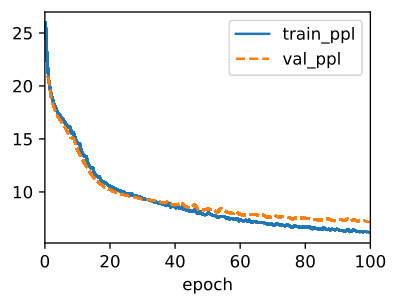
9.5.4. Training
Using The Time Machine dataset (data), we train a character-level language model (model) based on the RNN (rnn) implemented from scratch. Note that we first calculate the gradients, then clip them, and finally update the model parameters using the clipped gradients.
Time Machine 데이터 세트(데이터)를 사용하여 처음부터 구현된 RNN(rnn)을 기반으로 문자 수준 언어 모델(모델)을 교육합니다. 먼저 그래디언트를 계산한 다음 클리핑하고 마지막으로 클리핑된 그래디언트를 사용하여 모델 매개변수를 업데이트합니다.
data = d2l.TimeMachine(batch_size=1024, num_steps=32)
rnn = RNNScratch(num_inputs=len(data.vocab), num_hiddens=32)
model = RNNLMScratch(rnn, vocab_size=len(data.vocab), lr=1)
trainer = d2l.Trainer(max_epochs=100, gradient_clip_val=1, num_gpus=1)
trainer.fit(model, data)
위 코드는 'Time Machine' 데이터셋을 사용하여 RNN 기반의 언어 모델을 학습하는 과정을 나타냅니다.
- data = d2l.TimeMachine(batch_size=1024, num_steps=32): 이 코드는 'Time Machine' 데이터셋을 batch_size가 1024이고 num_steps가 32인 형태로 로드합니다. 이 데이터셋은 텍스트 데이터를 전처리하고 배치 형태로 구성하여 모델 학습에 사용될 준비를 합니다.
- rnn = RNNScratch(num_inputs=len(data.vocab), num_hiddens=32): RNNScratch 클래스의 인스턴스인 rnn을 생성합니다. 이 RNN 모델은 입력 차원을 len(data.vocab)으로, 은닉 상태 차원을 32로 설정합니다.
- model = RNNLMScratch(rnn, vocab_size=len(data.vocab), lr=1): RNNLMScratch 클래스의 인스턴스인 model을 생성합니다. 이 언어 모델은 앞서 생성한 rnn 모델을 기반으로 하며, 어휘 크기는 len(data.vocab)로 설정하고 학습률은 1로 설정합니다.
- trainer = d2l.Trainer(max_epochs=100, gradient_clip_val=1, num_gpus=1): Trainer 클래스의 인스턴스인 trainer를 생성합니다. 이 트레이너는 최대 100 에포크 동안 학습을 수행하며, 그레디언트 클리핑 임계값을 1로 설정하고 GPU 1개를 사용하여 학습합니다.
- trainer.fit(model, data): 생성한 trainer를 사용하여 모델 학습을 진행합니다. 학습 데이터는 data로 설정된 데이터셋을 사용하며, model이 학습됩니다.
요약하면, 위 코드는 'Time Machine' 데이터셋을 사용하여 RNN 기반의 언어 모델을 학습하는 과정을 나타내는 예제입니다.
9.5.5. Decoding
Once a language model has been learned, we can use it not only to predict the next token but to continue predicting each subsequent token, treating the previously predicted token as though it were the next token in the input. Sometimes we will just want to generate text as though we were starting at the beginning of a document. However, it is often useful to condition the language model on a user-supplied prefix. For example, if we were developing an autocomplete feature for search engine or to assist users in writing emails, we would want to feed in what they had written so far (the prefix), and then generate a likely continuation.
언어 모델이 학습되면 이를 사용하여 다음 토큰을 예측할 뿐만 아니라 각 후속 토큰을 계속 예측하여 이전에 예측한 토큰을 입력의 다음 토큰인 것처럼 처리할 수 있습니다. 때때로 우리는 문서의 시작 부분에서 시작하는 것처럼 텍스트를 생성하기를 원할 것입니다. 그러나 사용자가 제공한 접두사에서 언어 모델을 조건화하는 것이 종종 유용합니다. 예를 들어 검색 엔진용 자동 완성 기능을 개발하거나 사용자의 이메일 작성을 지원하는 경우 지금까지 작성한 내용(접두어)을 입력한 다음 가능성 있는 연속을 생성하려고 합니다.
The following predict method generates a continuation, one character at a time, after ingesting a user-provided prefix, When looping through the characters in prefix, we keep passing the hidden state to the next time step but do not generate any output. This is called the warm-up period. After ingesting the prefix, we are now ready to begin emitting the subsequent characters, each of which will be fed back into the model as the input at the subsequent time step.
다음 예측 메서드는 사용자가 제공한 접두사를 수집한 후 한 번에 한 문자씩 연속을 생성합니다. 접두사의 문자를 통해 반복할 때 숨겨진 상태를 다음 단계로 계속 전달하지만 출력을 생성하지는 않습니다. 이것을 워밍업 기간이라고 합니다. 접두사를 수집한 후 이제 후속 문자를 방출할 준비가 되었습니다. 각 문자는 후속 시간 단계에서 입력으로 모델에 피드백됩니다.
@d2l.add_to_class(RNNLMScratch)  #@save
def predict(self, prefix, num_preds, vocab, device=None):
    state, outputs = None, [vocab[prefix[0]]]
    for i in range(len(prefix) + num_preds - 1):
        X = torch.tensor([[outputs[-1]]], device=device)
        embs = self.one_hot(X)
        rnn_outputs, state = self.rnn(embs, state)
        if i < len(prefix) - 1:  # Warm-up period
            outputs.append(vocab[prefix[i + 1]])
        else:  # Predict num_preds steps
            Y = self.output_layer(rnn_outputs)
            outputs.append(int(Y.argmax(axis=2).reshape(1)))
    return ''.join([vocab.idx_to_token[i] for i in outputs])
위 코드는 RNN 기반 언어 모델에서 주어진 접두사(prefix)와 함께 이어지는 텍스트를 생성하는 predict 메서드를 정의하는 부분입니다.
- prefix: 초기 텍스트 접두사로, 이를 기반으로 이어지는 텍스트를 생성합니다.
- num_preds: 생성할 텍스트의 길이를 지정합니다.
- vocab: 사용할 어휘(단어 사전)를 나타냅니다.
- device: 텐서 연산을 수행할 디바이스를 지정합니다. 기본값은 None으로 CPU를 사용합니다.
메서드 내부에서는 다음과 같은 절차를 수행합니다:
- 초기 상태(state)와 초기 출력(outputs) 리스트를 설정합니다.
- 주어진 접두사의 첫 번째 단어를 출력 리스트에 추가합니다.
- 주어진 접두사로 모델을 warm-up(사전 훈련) 시키며, 훈련된 상태와 출력을 갱신합니다.
- prefix 이후로 텍스트를 생성합니다.
- 각 반복마다 이전 출력을 입력으로 사용하여 다음 단어를 예측합니다.
- 예측 결과에서 가장 높은 확률을 가진 단어를 선택하여 출력 리스트에 추가합니다.
- 최종적으로 출력 리스트에 추가된 단어들을 어휘의 인덱스로 변환하여 텍스트로 변환한 후 반환합니다.
이렇게 생성된 텍스트는 주어진 접두사와 모델의 예측을 조합하여 만들어진 것으로, 접두사 이후에 이어질 가능성이 높은 텍스트를 생성하는 역할을 합니다.
In the following, we specify the prefix and have it generate 20 additional characters.
다음에서는 접두사를 지정하고 20개의 추가 문자를 생성하도록 합니다.
model.predict('it has', 20, data.vocab, d2l.try_gpu())위 코드는 주어진 모델을 사용하여 주어진 접두사("it has")를 기반으로 텍스트를 생성하는 과정을 수행하는 부분입니다.
- model: 텍스트 생성에 사용할 RNN 기반 언어 모델입니다.
- prefix: 초기 텍스트 접두사로, 이를 기반으로 이어지는 텍스트를 생성합니다.
- num_preds: 생성할 텍스트의 길이를 지정합니다. 여기서는 20으로 설정되었습니다.
- vocab: 사용할 어휘(단어 사전)를 나타냅니다.
- device: 텐서 연산을 수행할 디바이스를 지정합니다.
이 메서드는 다음과 같이 작동합니다:
- 초기 상태와 출력 리스트를 설정합니다.
- 접두사의 각 단어를 입력으로 사용하여 초기 상태를 업데이트하고, 출력 리스트에 해당 단어를 추가합니다.
- warm-up 기간 동안 입력과 초기 상태를 사용하여 모델을 훈련하고, 상태와 출력을 갱신합니다.
- 접두사 이후로 텍스트를 생성합니다. 각 반복마다 이전 출력을 입력으로 사용하여 다음 단어를 예측하고, 예측 결과의 가장 높은 확률을 가진 단어를 출력 리스트에 추가합니다.
- 출력 리스트에 있는 단어들을 어휘의 인덱스로 변환하여 생성된 텍스트를 완성합니다.
이렇게 생성된 텍스트는 주어진 접두사("it has")를 기반으로 모델이 예측한 결과로 이루어진 것입니다. 이를 통해 모델이 언어의 패턴을 이해하고, 주어진 접두사에 어울리는 텍스트를 생성하도록 학습되었음을 확인할 수 있습니다.
'it has of the the the the '
While implementing the above RNN model from scratch is instructive, it is not convenient. In the next section, we will see how to leverage deep learning frameworks to whip up RNNs using standard architectures, and to reap performance gains by relying on highly optimized library functions.
위의 RNN 모델을 처음부터 구현하는 것은 유익하지만 편리하지는 않습니다. 다음 섹션에서는 딥 러닝 프레임워크를 활용하여 표준 아키텍처를 사용하여 RNN을 강화하고 고도로 최적화된 라이브러리 기능에 의존하여 성능 향상을 얻는 방법을 살펴보겠습니다.
9.5.6. Summary
We can train RNN-based language models to generate text following the user-provided text prefix. A simple RNN language model consists of input encoding, RNN modeling, and output generation. During training, gradient clipping can mitigate the problem of exploding gradients but does not address the problem of vanishing gradients. In the experiment, we implemented a simple RNN language model and trained it with gradient clipping on sequences of text, tokenized at the character level. By conditioning on a prefix, we can use a language model to generate likely continuations, which proves useful in many applications, e.g., autocomplete features.
사용자가 제공한 텍스트 접두사 다음에 텍스트를 생성하도록 RNN 기반 언어 모델을 훈련할 수 있습니다. 간단한 RNN 언어 모델은 입력 인코딩, RNN 모델링 및 출력 생성으로 구성됩니다. 교육 중에 그래디언트 클리핑은 그래디언트 폭발 문제를 완화할 수 있지만 그래디언트 소실 문제는 해결하지 못합니다. 실험에서 간단한 RNN 언어 모델을 구현하고 문자 수준에서 토큰화된 텍스트 시퀀스에서 그래디언트 클리핑으로 학습했습니다. 접두사를 조건으로 하여 언어 모델을 사용하여 가능한 연속을 생성할 수 있으며, 이는 자동 완성 기능과 같은 많은 응용 프로그램에서 유용합니다.
9.5.7. Exercises
- Does the implemented language model predict the next token based on all the past tokens up to the very first token in The Time Machine?
- Which hyperparameter controls the length of history used for prediction?
- Show that one-hot encoding is equivalent to picking a different embedding for each object.
- Adjust the hyperparameters (e.g., number of epochs, number of hidden units, number of time steps in a minibatch, and learning rate) to improve the perplexity. How low can you go while sticking with this simple architecture?
- Replace one-hot encoding with learnable embeddings. Does this lead to better performance?
- Conduct an experiment to determine how well this language model trained on The Time Machine works on other books by H. G. Wells, e.g., The War of the Worlds.
- Conduct another experiment to evaluate the perplexity of this model on books written by other authors.
'Dive into Deep Learning > D2L Recurrent Neural Networks (RNN)' 카테고리의 다른 글
| D2L - 9.7. Backpropagation Through Time (0) | 2023.08.02 |
|---|---|
| D2L - 9.6. Concise Implementation of Recurrent Neural Networks (0) | 2023.08.02 |
| D2L - 9.4. Recurrent Neural Networks (0) | 2023.08.02 |
| D2L - 9.3. Language Models (0) | 2023.08.02 |
| D2L - 9.2. Converting Raw Text into Sequence Data (0) | 2023.08.01 |
| D2L - 9.1. Working with Sequences (0) | 2023.08.01 |
| D2L - 9. Recurrent Neural Networks (0) | 2023.07.31 |