
3.5. Concise Implementation of Linear Regression
Deep learning has witnessed a sort of Cambrian explosion over the past decade. The sheer number of techniques, applications and algorithms by far surpasses the progress of previous decades. This is due to a fortuitous combination of multiple factors, one of which is the powerful free tools offered by a number of open-source deep learning frameworks. Theano (Bergstra et al., 2010), DistBelief (Dean et al., 2012), and Caffe (Jia et al., 2014) arguably represent the first generation of such models that found widespread adoption. In contrast to earlier (seminal) works like SN2 (Simulateur Neuristique) (Bottou and Le Cun, 1988), which provided a Lisp-like programming experience, modern frameworks offer automatic differentiation and the convenience of Python. These frameworks allow us to automate and modularize the repetitive work of implementing gradient-based learning algorithms.
딥러닝은 지난 10년 동안 일종의 캄브리아기 폭발을 목격했습니다. 기술, 응용 프로그램 및 알고리즘의 수는 지난 수십 년 동안의 발전을 훨씬 능가합니다. 이는 여러 요소의 우연한 조합으로 인해 발생하며, 그 중 하나는 수많은 오픈 소스 딥 러닝 프레임워크에서 제공하는 강력한 무료 도구입니다. Theano(Bergstra et al., 2010), DistBelief(Dean et al., 2012) 및 Caffe(Jia et al., 2014)는 틀림없이 널리 채택된 이러한 모델의 1세대를 대표합니다. Lisp와 같은 프로그래밍 경험을 제공한 SN2(Simulateur Neuristique)(Bottou and Le Cun, 1988)와 같은 이전(세미널) 작업과 달리 현대 프레임워크는 자동 차별화와 Python의 편리함을 제공합니다. 이러한 프레임워크를 사용하면 경사 기반 학습 알고리즘을 구현하는 반복적인 작업을 자동화하고 모듈화할 수 있습니다.
In Section 3.4, we relied only on (i) tensors for data storage and linear algebra; and (ii) automatic differentiation for calculating gradients. In practice, because data iterators, loss functions, optimizers, and neural network layers are so common, modern libraries implement these components for us as well. In this section, we will show you how to implement the linear regression model from Section 3.4 concisely by using high-level APIs of deep learning frameworks.
섹션 3.4에서는 (i) 데이터 저장 및 선형 대수학을 위한 텐서; (ii) 기울기 계산을 위한 자동 미분. 실제로 데이터 반복기, 손실 함수, 최적화 프로그램 및 신경망 계층은 매우 일반적이기 때문에 최신 라이브러리에서는 이러한 구성 요소도 구현합니다. 이번 섹션에서는 딥러닝 프레임워크의 고급 API를 사용하여 3.4절의 선형 회귀 모델을 간결하게 구현하는 방법을 보여드리겠습니다.
import numpy as np
import torch
from torch import nn
from d2l import torch as d2l
3.5.1. Defining the Model
When we implemented linear regression from scratch in Section 3.4, we defined our model parameters explicitly and coded up the calculations to produce output using basic linear algebra operations. You should know how to do this. But once your models get more complex, and once you have to do this nearly every day, you will be glad of the assistance. The situation is similar to coding up your own blog from scratch. Doing it once or twice is rewarding and instructive, but you would be a lousy web developer if you spent a month reinventing the wheel.
섹션 3.4에서 선형 회귀를 처음부터 구현했을 때 모델 매개변수를 명시적으로 정의하고 계산을 코딩하여 기본 선형 대수 연산을 사용하여 출력을 생성했습니다. 이 작업을 수행하는 방법을 알아야 합니다. 그러나 모델이 더욱 복잡해지고 거의 매일 이 작업을 수행해야 한다면 도움을 받게 되어 기쁠 것입니다. 상황은 처음부터 자신의 블로그를 코딩하는 것과 유사합니다. 한두 번 하는 것은 보람 있고 유익하지만 한 달 동안 바퀴를 재발명하는 데 소비한다면 당신은 형편없는 웹 개발자가 될 것입니다.
For standard operations, we can use a framework’s predefined layers, which allow us to focus on the layers used to construct the model rather than worrying about their implementation. Recall the architecture of a single-layer network as described in Fig. 3.1.2. The layer is called fully connected, since each of its inputs is connected to each of its outputs by means of a matrix–vector multiplication.
표준 작업의 경우 프레임워크의 사전 정의된 레이어를 사용할 수 있습니다. 이를 통해 구현에 대해 걱정하는 대신 모델을 구성하는 데 사용되는 레이어에 집중할 수 있습니다. 그림 3.1.2에 설명된 단일 계층 네트워크의 아키텍처를 떠올려보세요. 각 입력이 행렬-벡터 곱셈을 통해 각 출력에 연결되므로 이 레이어를 완전 연결이라고 합니다.
In PyTorch, the fully connected layer is defined in Linear and LazyLinear classes (available since version 1.8.0). The latter allows users to specify merely the output dimension, while the former additionally asks for how many inputs go into this layer. Specifying input shapes is inconvenient and may require nontrivial calculations (such as in convolutional layers). Thus, for simplicity, we will use such “lazy” layers whenever we can.
PyTorch에서 완전 연결 계층은 Linear 및 LazyLinear 클래스(버전 1.8.0부터 사용 가능)에 정의됩니다. 후자를 사용하면 사용자가 출력 차원만 지정할 수 있는 반면, 전자는 이 레이어에 들어가는 입력 수를 추가로 묻습니다. 입력 모양을 지정하는 것은 불편하며 컨볼루셔널 레이어와 같은 중요한 계산이 필요할 수 있습니다. 따라서 단순화를 위해 가능할 때마다 이러한 "게으른" 레이어를 사용하겠습니다.
class LinearRegression(d2l.Module):  #@save
    """The linear regression model implemented with high-level APIs."""
    def __init__(self, lr):
        super().__init__()
        self.save_hyperparameters()
        self.net = nn.LazyLinear(1)
        self.net.weight.data.normal_(0, 0.01)
        self.net.bias.data.fill_(0)
In the forward method we just invoke the built-in __call__ method of the predefined layers to compute the outputs.
전달 방법에서는 미리 정의된 레이어의 내장 __call__ 방법을 호출하여 출력을 계산합니다.
@d2l.add_to_class(LinearRegression)  #@save
def forward(self, X):
    return self.net(X)
3.5.2. Defining the Loss Function
The MSELoss class computes the mean squared error (without the 1/2 factor in (3.1.5)). By default, MSELoss returns the average loss over examples. It is faster (and easier to use) than implementing our own.
MSELoss 클래스는 평균 제곱 오차를 계산합니다((3.1.5)의 요소 없이). 기본적으로 MSELoss는 예제에 대한 평균 손실을 반환합니다. 자체적으로 구현하는 것보다 더 빠르고 사용하기 쉽습니다.
@d2l.add_to_class(LinearRegression)  #@save
def loss(self, y_hat, y):
    fn = nn.MSELoss()
    return fn(y_hat, y)
3.5.3. Defining the Optimization Algorithm
Minibatch SGD is a standard tool for optimizing neural networks and thus PyTorch supports it alongside a number of variations on this algorithm in the optim module. When we instantiate an SGD instance, we specify the parameters to optimize over, obtainable from our model via self.parameters(), and the learning rate (self.lr) required by our optimization algorithm.
Minibatch SGD는 신경망 최적화를 위한 표준 도구이므로 PyTorch는 최적화 모듈에서 이 알고리즘의 다양한 변형과 함께 이를 지원합니다. SGD 인스턴스를 인스턴스화할 때 최적화할 매개변수(self.parameters()를 통해 모델에서 얻을 수 있음)와 최적화 알고리즘에 필요한 학습 속도(self.lr)를 지정합니다.
@d2l.add_to_class(LinearRegression)  #@save
def configure_optimizers(self):
    return torch.optim.SGD(self.parameters(), self.lr)
3.5.4. Training
You might have noticed that expressing our model through high-level APIs of a deep learning framework requires fewer lines of code. We did not have to allocate parameters individually, define our loss function, or implement minibatch SGD. Once we start working with much more complex models, the advantages of the high-level API will grow considerably.
딥 러닝 프레임워크의 고급 API를 통해 모델을 표현하는 데 더 적은 코드 줄이 필요하다는 점을 눈치채셨을 것입니다. 매개변수를 개별적으로 할당하거나, 손실 함수를 정의하거나, 미니배치 SGD를 구현할 필요가 없었습니다. 훨씬 더 복잡한 모델로 작업을 시작하면 고급 API의 장점이 상당히 커질 것입니다.
Now that we have all the basic pieces in place, the training loop itself is the same as the one we implemented from scratch. So we just call the fit method (introduced in Section 3.2.4), which relies on the implementation of the fit_epoch method in Section 3.4, to train our model.
이제 모든 기본 부분이 준비되었으므로 훈련 루프 자체는 처음부터 구현한 것과 동일합니다. 따라서 우리는 모델을 훈련시키기 위해 섹션 3.4의 fit_epoch 메소드 구현에 의존하는 fit 메소드(섹션 3.2.4에 소개됨)를 호출합니다.
model = LinearRegression(lr=0.03)
data = d2l.SyntheticRegressionData(w=torch.tensor([2, -3.4]), b=4.2)
trainer = d2l.Trainer(max_epochs=3)
trainer.fit(model, data)

Below, we compare the model parameters learned by training on finite data and the actual parameters that generated our dataset. To access parameters, we access the weights and bias of the layer that we need. As in our implementation from scratch, note that our estimated parameters are close to their true counterparts.
아래에서는 유한 데이터를 훈련하여 학습한 모델 매개변수와 데이터세트를 생성한 실제 매개변수를 비교합니다. 매개변수에 액세스하려면 필요한 레이어의 가중치와 편향에 액세스합니다. 처음부터 구현하는 것처럼 추정된 매개변수는 실제 매개변수와 가깝습니다.
@d2l.add_to_class(LinearRegression)  #@save
def get_w_b(self):
    return (self.net.weight.data, self.net.bias.data)
w, b = model.get_w_b()

print(f'error in estimating w: {data.w - w.reshape(data.w.shape)}')
print(f'error in estimating b: {data.b - b}')
error in estimating w: tensor([ 0.0094, -0.0030])
error in estimating b: tensor([0.0137])
3.5.5. Summary
This section contains the first implementation of a deep network (in this book) to tap into the conveniences afforded by modern deep learning frameworks, such as MXNet (Chen et al., 2015), JAX (Frostig et al., 2018), PyTorch (Paszke et al., 2019), and Tensorflow (Abadi et al., 2016). We used framework defaults for loading data, defining a layer, a loss function, an optimizer and a training loop. Whenever the framework provides all necessary features, it is generally a good idea to use them, since the library implementations of these components tend to be heavily optimized for performance and properly tested for reliability. At the same time, try not to forget that these modules can be implemented directly. This is especially important for aspiring researchers who wish to live on the leading edge of model development, where you will be inventing new components that cannot possibly exist in any current library.
이 섹션에는 MXNet(Chen et al., 2015), JAX(Frostig et al., 2018), PyTorch와 같은 최신 딥 러닝 프레임워크가 제공하는 편리함을 활용하기 위한 딥 네트워크(이 책)의 첫 번째 구현이 포함되어 있습니다. (Paszke 외, 2019) 및 Tensorflow(Abadi 외, 2016). 데이터 로드, 레이어 정의, 손실 함수, 최적화 프로그램 및 훈련 루프에 프레임워크 기본값을 사용했습니다. 프레임워크가 필요한 모든 기능을 제공할 때마다 일반적으로 이를 사용하는 것이 좋습니다. 이러한 구성 요소의 라이브러리 구현은 성능에 대해 크게 최적화되고 안정성에 대해 적절하게 테스트되는 경향이 있기 때문입니다. 동시에 이러한 모듈을 직접 구현할 수 있다는 점을 잊지 마십시오. 이는 현재 어떤 라이브러리에도 존재할 수 없는 새로운 구성 요소를 발명하게 될 모델 개발의 선두에 서기를 원하는 야심찬 연구자에게 특히 중요합니다.
In PyTorch, the data module provides tools for data processing, the nn module defines a large number of neural network layers and common loss functions. We can initialize the parameters by replacing their values with methods ending with _. Note that we need to specify the input dimensions of the network. While this is trivial for now, it can have significant knock-on effects when we want to design complex networks with many layers. Careful considerations of how to parametrize these networks is needed to allow portability.
PyTorch에서 데이터 모듈은 데이터 처리를 위한 도구를 제공하고, nn 모듈은 수많은 신경망 계층과 일반적인 손실 함수를 정의합니다. 매개변수 값을 _로 끝나는 메소드로 대체하여 매개변수를 초기화할 수 있습니다. 네트워크의 입력 차원을 지정해야 합니다. 지금은 이것이 사소한 일이지만, 많은 레이어로 구성된 복잡한 네트워크를 설계할 때 상당한 연쇄 효과를 가질 수 있습니다. 이식성을 허용하려면 이러한 네트워크를 매개변수화하는 방법에 대한 신중한 고려가 필요합니다.
3.5.6. Exercises

https://ko.d2l.ai/chapter_deep-learning-basics/fashion-mnist.html
3.5. 이미지 분류 데이터 (Fashion-MNIST) — Dive into Deep Learning documentation
ko.d2l.ai
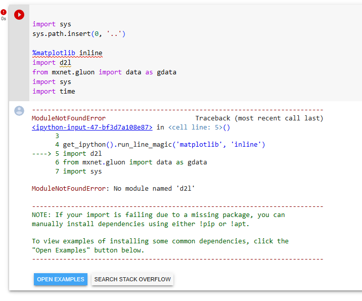
D2L 모듈이 인스톨 되지 않아 소스 코드들을 실행 할 수 없음


'Dive into Deep Learning > D2L Linear Neural Networks' 카테고리의 다른 글
| D2L - 4.3. The Base Classification Model (0) | 2023.06.26 |
|---|---|
| D2L - 4.2. The Image Classification Dataset (0) | 2023.06.26 |
| D2L 4.1. Softmax Regression (1) | 2023.06.26 |
| D2L - 4. Linear Neural Networks for Classification (0) | 2023.06.26 |
| D2L - Local Environment Setting (0) | 2023.06.26 |
| D2L - 3.4. Linear Regression Implementation from Scratch , Softmax 회귀(regression) (0) | 2023.06.22 |
| D2L - 3.3. Synthetic Regression Data (0) | 2023.06.22 |
| D2L 3.2. Object-Oriented Design for Implementation (0) | 2023.06.22 |
| D2L 3.2. 선형 회귀를 처음부터 구현하기 (0) | 2023.06.22 |
| D2L 3.1. Linear Regression (0) | 2023.06.20 |