

D2L - 3.3. Synthetic Regression Data
2023. 6. 22. 03:36 |
https://d2l.ai/chapter_linear-regression/synthetic-regression-data.html
3.3. Synthetic Regression Data — Dive into Deep Learning 1.0.3 documentation
d2l.ai
Machine learning is all about extracting information from data. So you might wonder, what could we possibly learn from synthetic data? While we might not care intrinsically about the patterns that we ourselves baked into an artificial data generating model, such datasets are nevertheless useful for didactic purposes, helping us to evaluate the properties of our learning algorithms and to confirm that our implementations work as expected. For example, if we create data for which the correct parameters are known a priori, then we can check that our model can in fact recover them.
머신러닝은 데이터에서 정보를 추출하는 것입니다. 그렇다면 합성 데이터에서 무엇을 배울 수 있을지 궁금할 것입니다. 우리는 인공 데이터 생성 모델에 직접 적용한 패턴에 본질적으로 관심을 두지 않을 수도 있지만 그럼에도 불구하고 이러한 데이터 세트는 교훈적인 목적으로 유용하며 학습 알고리즘의 속성을 평가하고 구현이 예상대로 작동하는지 확인하는 데 도움이 됩니다. 예를 들어, 올바른 매개변수가 선험적으로 알려진 데이터를 생성하는 경우 모델이 실제로 해당 매개변수를 복구할 수 있는지 확인할 수 있습니다.
%matplotlib inline
import random
import torch
from d2l import torch as d2l
3.3.1. Generating the Dataset
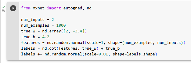
For this example, we will work in low dimension for succinctness. The following code snippet generates 1000 examples with 2-dimensional features drawn from a standard normal distribution. The resulting design matrix X belongs to ℝ **1000×2. We generate each label by applying a ground truth linear function, corrupting them via additive noise ϵ , drawn independently and identically for each example:
이 예에서는 간결성을 위해 낮은 차원에서 작업하겠습니다. 다음 코드 조각은 표준 정규 분포에서 추출된 2차원 특징을 사용하여 1000개의 예를 생성합니다. 결과 설계 행렬 X는 ℝ **1000×2에 속합니다. 우리는 Ground Truth 선형 함수를 적용하여 각 라벨을 생성하고, 각 예에 대해 독립적이고 동일하게 그려진 추가 노이즈 ϵ 를 통해 라벨을 손상시킵니다.

For convenience we assume that ϵ is drawn from a normal distribution with mean μ =0 and standard deviation σ =0.01. Note that for object-oriented design we add the code to the __init__ method of a subclass of d2l.DataModule (introduced in Section 3.2.3). It is good practice to allow the setting of any additional hyperparameters. We accomplish this with save_hyperparameters(). The batch_size will be determined later.
편의상 ϵ는 평균 μ =0이고 표준편차 σ =0.01인 정규 분포에서 도출되었다고 가정합니다. 객체 지향 설계의 경우 d2l.DataModule 하위 클래스의 __init__ 메서드에 코드를 추가합니다(섹션 3.2.3에 소개됨). 추가 하이퍼파라미터 설정을 허용하는 것이 좋습니다. save_hyperparameters()를 사용하여 이를 수행합니다. Batch_size는 나중에 결정됩니다.
class SyntheticRegressionData(d2l.DataModule):  #@save
    """Synthetic data for linear regression."""
    def __init__(self, w, b, noise=0.01, num_train=1000, num_val=1000,
                 batch_size=32):
        super().__init__()
        self.save_hyperparameters()
        n = num_train + num_val
        self.X = torch.randn(n, len(w))
        noise = torch.randn(n, 1) * noise
        self.y = torch.matmul(self.X, w.reshape((-1, 1))) + b + noise
Below, we set the true parameters to w=[2,−3.4]⊤ and b=4.2. Later, we can check our estimated parameters against these ground truth values.
아래에서는 실제 매개변수를 w=[2,−3.4]⊤ 및 b=4.2로 설정했습니다. 나중에 이러한 실제 값과 비교하여 추정된 매개변수를 확인할 수 있습니다.
data = SyntheticRegressionData(w=torch.tensor([2, -3.4]), b=4.2)
Each row in features consists of a vector in ℝ**2 and each row in labels is a scalar. Let’s have a look at the first entry.
특성의 각 행은 ℝ**2의 벡터로 구성되고 레이블의 각 행은 스칼라입니다. 첫 번째 항목을 살펴보겠습니다.
print('features:', data.X[0],'\nlabel:', data.y[0])features: tensor([0.9026, 1.0264])
label: tensor([2.5148])
3.3.2. Reading the Dataset
Training machine learning models often requires multiple passes over a dataset, grabbing one minibatch of examples at a time. This data is then used to update the model. To illustrate how this works, we implement the get_dataloader method, registering it in the SyntheticRegressionData class via add_to_class (introduced in Section 3.2.1). It takes a batch size, a matrix of features, and a vector of labels, and generates minibatches of size batch_size. As such, each minibatch consists of a tuple of features and labels. Note that we need to be mindful of whether we’re in training or validation mode: in the former, we will want to read the data in random order, whereas for the latter, being able to read data in a pre-defined order may be important for debugging purposes.
기계 학습 모델을 훈련하려면 한 번에 하나의 미니 배치 예제를 가져오는 데이터 세트에 대한 여러 번의 전달이 필요한 경우가 많습니다. 그런 다음 이 데이터는 모델을 업데이트하는 데 사용됩니다. 이것이 어떻게 작동하는지 설명하기 위해 get_dataloader 메소드를 구현하고 이를 add_to_class를 통해 SyntheticRegressionData 클래스에 등록합니다(섹션 3.2.1에 소개됨). 배치 크기, 기능 매트릭스, 레이블 벡터를 사용하고 배치_크기 크기의 미니 배치를 생성합니다. 따라서 각 미니 배치는 기능과 레이블의 튜플로 구성됩니다. 훈련 모드에 있는지 검증 모드에 있는지 주의해야 합니다. 전자에서는 데이터를 무작위 순서로 읽으려는 반면, 후자의 경우 미리 정의된 순서로 데이터를 읽을 수 있으면 디버깅 목적으로 중요합니다.
@d2l.add_to_class(SyntheticRegressionData)
def get_dataloader(self, train):
    if train:
        indices = list(range(0, self.num_train))
        # The examples are read in random order
        random.shuffle(indices)
    else:
        indices = list(range(self.num_train, self.num_train+self.num_val))
    for i in range(0, len(indices), self.batch_size):
        batch_indices = torch.tensor(indices[i: i+self.batch_size])
        yield self.X[batch_indices], self.y[batch_indices]
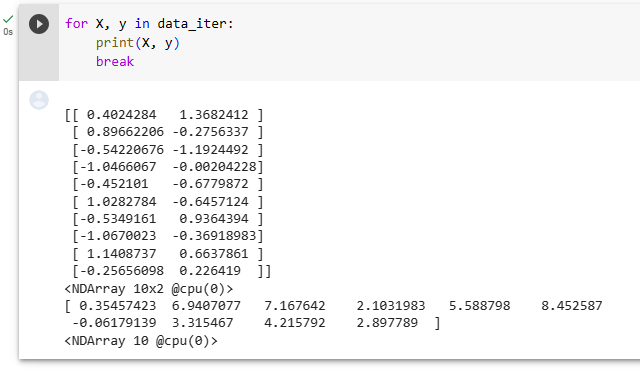
To build some intuition, let’s inspect the first minibatch of data. Each minibatch of features provides us with both its size and the dimensionality of input features. Likewise, our minibatch of labels will have a matching shape given by batch_size.
직관력을 키우기 위해 첫 번째 데이터 미니 배치를 살펴보겠습니다. 각 기능의 미니 배치는 입력 기능의 크기와 차원을 모두 제공합니다. 마찬가지로, 우리의 라벨 미니 배치는 배치_크기에 따라 일치하는 모양을 갖습니다.
X, y = next(iter(data.train_dataloader()))
print('X shape:', X.shape, '\ny shape:', y.shape)
X shape: torch.Size([32, 2])
y shape: torch.Size([32, 1])
While seemingly innocuous, the invocation of iter(data.train_dataloader()) illustrates the power of Python’s object-oriented design. Note that we added a method to the SyntheticRegressionData class after creating the data object. Nonetheless, the object benefits from the ex post facto addition of functionality to the class.
겉으로는 무해해 보이지만 iter(data.train_dataloader())의 호출은 Python의 객체 지향 설계의 힘을 보여줍니다. 데이터 객체를 생성한 후 SyntheticRegressionData 클래스에 메서드를 추가했습니다. 그럼에도 불구하고 객체는 사후에 클래스에 기능을 추가함으로써 이점을 얻습니다.
Throughout the iteration we obtain distinct minibatches until the entire dataset has been exhausted (try this). While the iteration implemented above is good for didactic purposes, it is inefficient in ways that might get us into trouble with real problems. For example, it requires that we load all the data in memory and that we perform lots of random memory access. The built-in iterators implemented in a deep learning framework are considerably more efficient and they can deal with sources such as data stored in files, data received via a stream, and data generated or processed on the fly. Next let’s try to implement the same method using built-in iterators.
반복을 통해 전체 데이터 세트가 소진될 때까지 별도의 미니 배치를 얻습니다(이것을 시도하십시오). 위에 구현된 반복은 교훈적인 목적으로는 좋지만 실제 문제를 해결할 수 있다는 점에서는 비효율적입니다. 예를 들어, 모든 데이터를 메모리에 로드하고 많은 무작위 메모리 액세스를 수행해야 합니다. 딥 러닝 프레임워크에 구현된 내장 반복자는 훨씬 더 효율적이며 파일에 저장된 데이터, 스트림을 통해 수신된 데이터, 즉석에서 생성되거나 처리되는 데이터와 같은 소스를 처리할 수 있습니다. 다음으로 내장된 반복자를 사용하여 동일한 메서드를 구현해 보겠습니다.
3.3.3. Concise Implementation of the Data Loade
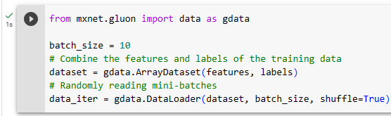
Rather than writing our own iterator, we can call the existing API in a framework to load data. As before, we need a dataset with features X and labels y. Beyond that, we set batch_size in the built-in data loader and let it take care of shuffling examples efficiently.
자체 반복자를 작성하는 대신 프레임워크에서 기존 API를 호출하여 데이터를 로드할 수 있습니다. 이전과 마찬가지로 특성 X와 레이블 y가 있는 데이터 세트가 필요합니다. 그 외에도 내장 데이터 로더에서 배치_크기를 설정하고 셔플링 예제를 효율적으로 처리하도록 했습니다.
@d2l.add_to_class(d2l.DataModule)  #@save
def get_tensorloader(self, tensors, train, indices=slice(0, None)):
    tensors = tuple(a[indices] for a in tensors)
    dataset = torch.utils.data.TensorDataset(*tensors)
    return torch.utils.data.DataLoader(dataset, self.batch_size,
                                       shuffle=train)

@d2l.add_to_class(SyntheticRegressionData)  #@save
def get_dataloader(self, train):
    i = slice(0, self.num_train) if train else slice(self.num_train, None)
    return self.get_tensorloader((self.X, self.y), train, i)
The new data loader behaves just like the previous one, except that it is more efficient and has some added functionality.
새로운 데이터 로더는 더 효율적이고 몇 가지 추가 기능이 있다는 점을 제외하면 이전 데이터 로더와 동일하게 작동합니다.
X, y = next(iter(data.train_dataloader()))
print('X shape:', X.shape, '\ny shape:', y.shape)
X shape: torch.Size([32, 2])
y shape: torch.Size([32, 1])
For instance, the data loader provided by the framework API supports the built-in __len__ method, so we can query its length, i.e., the number of batches.
예를 들어 프레임워크 API에서 제공하는 데이터 로더는 내장된 __len__ 메서드를 지원하므로 해당 길이, 즉 배치 수를 쿼리할 수 있습니다.
len(data.train_dataloader())32
3.3.4. Summary
Data loaders are a convenient way of abstracting out the process of loading and manipulating data. This way the same machine learning algorithm is capable of processing many different types and sources of data without the need for modification. One of the nice things about data loaders is that they can be composed. For instance, we might be loading images and then have a postprocessing filter that crops them or modifies them in other ways. As such, data loaders can be used to describe an entire data processing pipeline.
데이터 로더는 데이터 로드 및 조작 프로세스를 추상화하는 편리한 방법입니다. 이러한 방식으로 동일한 기계 학습 알고리즘은 수정 없이도 다양한 유형과 데이터 소스를 처리할 수 있습니다. 데이터 로더의 좋은 점 중 하나는 구성이 가능하다는 것입니다. 예를 들어 이미지를 로드한 다음 이미지를 자르거나 다른 방식으로 수정하는 후처리 필터를 사용할 수 있습니다. 따라서 데이터 로더를 사용하여 전체 데이터 처리 파이프라인을 설명할 수 있습니다.
As for the model itself, the two-dimensional linear model is about the simplest we might encounter. It lets us test out the accuracy of regression models without worrying about having insufficient amounts of data or an underdetermined system of equations. We will put this to good use in the next section.
모델 자체에 관해서는 2차원 선형 모델이 우리가 접할 수 있는 가장 간단한 모델입니다. 이를 통해 데이터 양이 부족하거나 방정식 시스템이 불충분하게 결정되는 것에 대한 걱정 없이 회귀 모델의 정확성을 테스트할 수 있습니다. 다음 섹션에서 이를 잘 활용하겠습니다.
3.3.5. Exercises
- What will happen if the number of examples cannot be divided by the batch size. How would you change this behavior by specifying a different argument by using the framework’s API?
- Suppose that we want to generate a huge dataset, where both the size of the parameter vector w and the number of examples num_examples are large.
- What happens if we cannot hold all data in memory?
- How would you shuffle the data if it is held on disk? Your task is to design an efficient algorithm that does not require too many random reads or writes. Hint: pseudorandom permutation generators allow you to design a reshuffle without the need to store the permutation table explicitly (Naor and Reingold, 1999).
- Implement a data generator that produces new data on the fly, every time the iterator is called.
- How would you design a random data generator that generates the same data each time it is called?
https://ko.d2l.ai/chapter_deep-learning-basics/linear-regression-gluon.html
3.3. 선형 회귀의 간결한 구현 — Dive into Deep Learning documentation
ko.d2l.ai


'Dive into Deep Learning > D2L Linear Neural Networks' 카테고리의 다른 글
| D2L - 4.3. The Base Classification Model (0) | 2023.06.26 |
|---|---|
| D2L - 4.2. The Image Classification Dataset (0) | 2023.06.26 |
| D2L 4.1. Softmax Regression (1) | 2023.06.26 |
| D2L - 4. Linear Neural Networks for Classification (0) | 2023.06.26 |
| D2L - Local Environment Setting (0) | 2023.06.26 |
| D2L - 3.5. Concise Implementation of Linear Regression, 이미지 분류 데이터 (Fashion-MNIST) (0) | 2023.06.22 |
| D2L - 3.4. Linear Regression Implementation from Scratch , Softmax 회귀(regression) (0) | 2023.06.22 |
| D2L 3.2. Object-Oriented Design for Implementation (0) | 2023.06.22 |
| D2L 3.2. 선형 회귀를 처음부터 구현하기 (0) | 2023.06.22 |
| D2L 3.1. Linear Regression (0) | 2023.06.20 |