

5.2. Implementation of Multilayer Perceptrons — Dive into Deep Learning 1.0.0-beta0 documentation
d2l.ai
5.2. Implementation of Multilayer Perceptrons
Multilayer perceptrons (MLPs) are not much more complex to implement than simple linear models. The key conceptual difference is that we now concatenate multiple layers.
다층 퍼셉트론(MLP)은 단순한 선형 모델보다 구현하기가 많이 복잡하지 않습니다. 주요 개념적 차이점은 이제 여러 레이어를 연결한다는 것입니다.
import torch
from torch import nn
from d2l import torch as d2l
위 코드는 torch, torch.nn, 그리고 d2l 패키지를 임포트하는 예시입니다.
- torch: PyTorch의 기본 패키지로, 다양한 텐서 연산과 딥러닝 모델 구성을 위한 도구들을 제공합니다.
- torch.nn: PyTorch의 신경망 관련 모듈을 포함한 패키지로, 신경망 레이어, 활성화 함수, 손실 함수 등을 정의하고 제공합니다.
- d2l.torch: d2l 패키지에서 제공하는 PyTorch 관련 유틸리티 함수와 클래스들을 포함한 모듈입니다. 이 모듈은 d2l 패키지의 torch 모듈에 대한 별칭(Alias)로 사용됩니다.
해당 코드에서는 이러한 패키지와 모듈을 임포트하여 사용할 준비를 하고 있습니다. 이후 코드에서는 해당 패키지와 모듈의 함수와 클래스를 사용하여 신경망 모델을 정의하고 학습하는 등의 작업을 수행할 수 있습니다.
5.2.1. Implementation from Scratch
Let’s begin again by implementing such a network from scratch.
이러한 네트워크를 처음부터 다시 구현해 보겠습니다.
5.2.1.1. Initializing Model Parameters
Recall that Fashion-MNIST contains 10 classes, and that each image consists of a 28×28=784 grid of grayscale pixel values. As before we will disregard the spatial structure among the pixels for now, so we can think of this as a classification dataset with 784 input features and 10 classes. To begin, we will implement an MLP with one hidden layer and 256 hidden units. Both the number of layers and their width are adjustable (they are considered hyperparameters). Typically, we choose the layer widths to be divisible by larger powers of 2. This is computationally efficient due to the way memory is allocated and addressed in hardware.
Fashion-MNIST에는 10개의 클래스가 포함되어 있고 각 이미지는 그레이스케일 픽셀 값의 28X28=784 그리드로 구성되어 있습니다. 이전과 마찬가지로 지금은 픽셀 간의 공간 구조를 무시하므로 784개의 입력 기능과 10개의 클래스가 있는 분류 데이터 세트로 생각할 수 있습니다. 시작하려면 하나의 숨겨진 레이어와 256개의 숨겨진 유닛이 있는 MLP를 구현합니다. 레이어 수와 너비는 모두 조정 가능합니다(하이퍼 매개변수로 간주됨). 일반적으로 더 큰 2의 거듭제곱으로 나눌 수 있는 레이어 너비를 선택합니다. 이것은 하드웨어에서 메모리가 할당되고 주소 지정되는 방식으로 인해 계산상 효율적입니다.
Again, we will represent our parameters with several tensors. Note that for every layer, we must keep track of one weight matrix and one bias vector. As always, we allocate memory for the gradients of the loss with respect to these parameters.
다시 한 번 여러 텐서로 매개변수를 나타냅니다. 모든 레이어에 대해 하나의 가중치 행렬과 하나의 편향 벡터를 추적해야 합니다. 항상 그렇듯이 이러한 매개변수와 관련하여 손실 기울기에 대한 메모리를 할당합니다.
In the code below we use `nn.Parameter <https://pytorch.org/docs/stable/generated/torch.nn.parameter.Parameter.html>`__ to automatically register a class attribute as a parameter to be tracked by autograd (Section 2.5).
아래 코드에서 `nn.Parameter <https://pytorch.org/docs/stable/generated/torch.nn.parameter.Parameter.html>`__를 사용하여 클래스 속성을 autograd에 의해 추적할 매개변수로 자동 등록합니다. (섹션 2.5).
class MLPScratch(d2l.Classifier):
    def __init__(self, num_inputs, num_outputs, num_hiddens, lr, sigma=0.01):
        super().__init__()
        self.save_hyperparameters()
        self.W1 = nn.Parameter(torch.randn(num_inputs, num_hiddens) * sigma)
        self.b1 = nn.Parameter(torch.zeros(num_hiddens))
        self.W2 = nn.Parameter(torch.randn(num_hiddens, num_outputs) * sigma)
        self.b2 = nn.Parameter(torch.zeros(num_outputs))
위 코드는 MLPScratch 클래스를 정의하는 예시입니다. 이 클래스는 d2l.Classifier 클래스를 상속받아 다층 퍼셉트론(MLP) 모델을 Scratch로 구현하는 역할을 합니다.
- num_inputs: 입력 특성의 개수입니다.
- num_outputs: 출력 클래스의 개수입니다.
- num_hiddens: 은닉층의 유닛 개수입니다.
- lr: 학습률(learning rate)입니다.
- sigma: 가중치 초기화에 사용되는 표준 편차입니다.
MLPScratch 클래스의 __init__ 메서드에서는 모델의 매개변수를 초기화하는 작업을 수행합니다. 다음과 같은 매개변수들을 정의하고 초기화합니다:
- W1: 입력층과 첫 번째 은닉층 사이의 가중치 행렬입니다. 크기는 (num_inputs, num_hiddens)이며, 정규 분포로부터 무작위로 초기화됩니다.
- b1: 첫 번째 은닉층의 편향 벡터입니다. 크기는 (num_hiddens,)이며, 모든 요소가 0으로 초기화됩니다.
- W2: 첫 번째 은닉층과 출력층 사이의 가중치 행렬입니다. 크기는 (num_hiddens, num_outputs)이며, 정규 분포로부터 무작위로 초기화됩니다.
- b2: 출력층의 편향 벡터입니다. 크기는 (num_outputs,)이며, 모든 요소가 0으로 초기화됩니다.
이렇게 초기화된 매개변수들은 모델의 일부가 되며, 학습 과정에서 업데이트되어 모델이 데이터를 잘 학습할 수 있도록 합니다.
5.2.1.2. Model
To make sure we know how everything works, we will implement the ReLU activation ourselves rather than invoking the built-in relu function directly.
모든 것이 어떻게 작동하는지 확인하기 위해 내장된 relu 함수를 직접 호출하는 대신 ReLU 활성화를 직접 구현합니다.
def relu(X):
    a = torch.zeros_like(X)
    return torch.max(X, a)
위 코드는 ReLU(Recitified Linear Unit) 활성화 함수인 relu 함수를 정의하는 예시입니다.
ReLU 함수는 입력으로 받은 텐서 X의 각 원소에 대해 양수인 경우는 그대로 출력하고, 음수인 경우는 0으로 변환하여 반환합니다.
함수 내부에서는 torch.zeros_like 함수를 사용하여 X와 동일한 크기의 텐서 a를 생성합니다. 이후 torch.max 함수를 사용하여 X와 a의 원소별로 최댓값을 계산합니다. 이때, a의 모든 원소는 0이므로, X의 각 원소가 양수인 경우는 X의 해당 원소가 그대로 출력되고, 음수인 경우는 0으로 변환됩니다.
ReLU 함수는 주로 신경망 모델에서 은닉층의 활성화 함수로 사용되며, 비선형성을 추가하여 모델의 표현력을 향상시킵니다.
Since we are disregarding spatial structure, we reshape each two-dimensional image into a flat vector of length num_inputs. Finally, we implement our model with just a few lines of code. Since we use the framework built-in autograd this is all that it takes.
우리는 공간 구조를 무시하고 있기 때문에 각 2차원 이미지를 길이가 num_inputs인 평면 벡터로 재구성합니다. 마지막으로 몇 줄의 코드만으로 모델을 구현합니다. 프레임워크에 내장된 autograd를 사용하기 때문에 이것이 전부입니다.
@d2l.add_to_class(MLPScratch)
def forward(self, X):
    X = X.reshape((-1, self.num_inputs))
    H = relu(torch.matmul(X, self.W1) + self.b1)
    return torch.matmul(H, self.W2) + self.b2
위 코드는 MLPScratch 클래스에 forward 메서드를 추가하는 예시입니다.
forward 메서드는 입력 데이터 X를 받아 신경망의 순전파 연산을 수행하는 역할을 합니다.
먼저, 입력 데이터 X의 크기를 (배치 크기, 입력 차원 수)로 변형합니다. 이는 입력 데이터를 배치로 처리하기 위한 조치입니다.
다음으로, 입력 데이터 X와 첫 번째 가중치 행렬 self.W1을 행렬 곱하고 편향 벡터 self.b1을 더합니다. 그리고 결과에 ReLU 활성화 함수를 적용한 결과를 H에 저장합니다. 이렇게 하면 입력 데이터가 첫 번째 은닉층을 통과한 출력이 얻어집니다.
마지막으로, H와 두 번째 가중치 행렬 self.W2를 행렬 곱하고 편향 벡터 self.b2를 더합니다. 이를 통해 은닉층의 출력인 H가 두 번째 가중치를 통과하여 최종 출력이 계산됩니다.
따라서, forward 메서드의 반환값은 신경망의 순전파 연산을 통해 계산된 예측 결과입니다.
5.2.1.3. Training
Fortunately, the training loop for MLPs is exactly the same as for softmax regression. We define the model, data, trainer and finally invoke the fit method on model and data.
다행스럽게도 MLP의 훈련 루프는 softmax 회귀와 정확히 동일합니다. 우리는 모델, 데이터, 트레이너를 정의하고 마지막으로 모델과 데이터에 맞는 메서드를 호출합니다.
model = MLPScratch(num_inputs=784, num_outputs=10, num_hiddens=256, lr=0.1)
data = d2l.FashionMNIST(batch_size=256)
trainer = d2l.Trainer(max_epochs=10)
trainer.fit(model, data)
위 코드는 MLPScratch 모델을 생성하고 FashionMNIST 데이터셋을 사용하여 모델을 훈련시키는 예시입니다.
먼저, MLPScratch 클래스를 사용하여 model 객체를 생성합니다. 이 때, 입력 차원 수를 784, 출력 차원 수를 10으로 설정하고, 은닉층의 뉴런 수를 256으로 설정합니다. 또한, 학습률을 0.1로 설정합니다.
다음으로, d2l.FashionMNIST를 사용하여 data 객체를 생성합니다. 이 객체는 FashionMNIST 데이터셋을 나타내며, 배치 크기를 256으로 설정합니다.
마지막으로, d2l.Trainer를 사용하여 trainer 객체를 생성합니다. trainer 객체는 모델을 훈련시키는 역할을 수행합니다. 이 때, 최대 에포크 수를 10으로 설정합니다.
trainer.fit(model, data)를 호출하여 모델을 주어진 데이터로 훈련시킵니다. 이는 모델의 가중치와 편향을 최적화하기 위한 학습 과정을 수행하는 것입니다. 훈련 후, 최적화된 모델의 성능을 평가하거나 예측을 수행할 수 있습니다.

5.2.2. Concise Implementation
As you might expect, by relying on the high-level APIs, we can implement MLPs even more concisely.
예상할 수 있듯이 상위 수준 API에 의존하여 MLP를 훨씬 더 간결하게 구현할 수 있습니다.
5.2.2.1. Model
As compared with our concise implementation of softmax regression implementation (Section 4.5), the only difference is that we add two fully connected layers where we previously added only one. The first is the hidden layer, the second is the output layer.
softmax 회귀 구현의 간결한 구현(섹션 4.5)과 비교할 때 유일한 차이점은 이전에 하나만 추가한 두 개의 완전히 연결된 레이어를 추가한다는 것입니다. 첫 번째는 숨겨진 레이어이고 두 번째는 출력 레이어입니다.
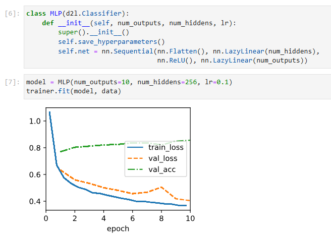
class MLP(d2l.Classifier):
    def __init__(self, num_outputs, num_hiddens, lr):
        super().__init__()
        self.save_hyperparameters()
        self.net = nn.Sequential(nn.Flatten(), nn.LazyLinear(num_hiddens),
                                 nn.ReLU(), nn.LazyLinear(num_outputs))
위 코드는 MLP (다층 퍼셉트론) 모델을 구성하는 클래스인 MLP를 정의하는 예시입니다.
MLP 클래스는 d2l.Classifier 클래스를 상속받아 MLP 모델을 구현합니다. 모델의 출력 차원 수인 num_outputs, 은닉층의 뉴런 수인 num_hiddens, 그리고 학습률인 lr을 초기화 인자로 받습니다.
__init__ 메서드에서는 모델의 구조를 정의합니다. nn.Sequential을 사용하여 여러 개의 층을 차례로 쌓아서 모델을 구성합니다. 첫 번째 층으로는 nn.Flatten()을 사용하여 입력 데이터를 1차원으로 펼치는 작업을 수행합니다. 두 번째 층은 nn.LazyLinear(num_hiddens)로 정의되어 있으며, 은닉층으로 작용합니다. 활성화 함수로는 ReLU 함수인 nn.ReLU()를 사용합니다. 마지막 층은 nn.LazyLinear(num_outputs)로 정의되어 있으며, 출력층으로 작용합니다.
이렇게 정의된 MLP 클래스는 입력 데이터를 받아 순전파 연산을 수행하여 모델의 출력값을 계산합니다. 모델의 학습과 평가는 d2l.Trainer 클래스를 사용하여 수행할 수 있습니다.
Previously, we defined forward methods for models to transform input using the model parameters. These operations are essentially a pipeline: you take an input and apply a transformation (e.g., matrix multiplication with weights followed by bias addition), then repetitively use the output of the current transformation as input to the next transformation. However, you may have noticed that no forward method is defined here. In fact, MLP inherits the forward method from the Module class (Section 3.2.2) to simply invoke self.net(X) (X is input), which is now defined as a sequence of transformations via the Sequential class. The Sequential class abstracts the forward process enabling us to focus on the transformations. We will further discuss how the Sequential class works in Section 6.1.2.
이전에는 모델 매개변수를 사용하여 입력을 변환하는 모델에 대한 전달 방법을 정의했습니다. 이러한 작업은 본질적으로 파이프라인입니다. 입력을 받고 변환(예: 가중치를 사용한 행렬 곱셈과 바이어스 추가)을 적용한 다음 현재 변환의 출력을 다음 변환에 대한 입력으로 반복적으로 사용합니다. 그러나 여기에 정방향 방법이 정의되어 있지 않음을 알 수 있습니다. 실제로 MLP는 Sequential 클래스를 통한 일련의 변환으로 정의된 self.net(X)(X가 입력됨)을 호출하기 위해 Module 클래스(섹션 3.2.2)에서 전달 메서드를 상속합니다. Sequential 클래스는 변환에 집중할 수 있도록 전달 프로세스를 추상화합니다. 섹션 6.1.2에서 Sequential 클래스의 작동 방식에 대해 자세히 설명합니다.
5.2.2.2. Training
The training loop is exactly the same as when we implemented softmax regression. This modularity enables us to separate matters concerning the model architecture from orthogonal considerations.
학습 루프는 softmax 회귀를 구현했을 때와 정확히 동일합니다. 이러한 모듈성을 통해 모델 아키텍처와 관련된 문제를 직교 고려 사항에서 분리할 수 있습니다.
model = MLP(num_outputs=10, num_hiddens=256, lr=0.1)
trainer.fit(model, data)
위 코드는 MLP 클래스를 사용하여 MLP 모델을 생성하고, d2l.Trainer를 사용하여 모델을 학습하는 예시입니다.
MLP 클래스의 인스턴스인 model을 생성할 때, 출력 차원 수 num_outputs를 10, 은닉층의 뉴런 수 num_hiddens를 256, 학습률 lr을 0.1로 설정합니다.
trainer.fit(model, data)는 d2l.Trainer를 사용하여 모델을 학습하는 부분입니다. model은 학습할 모델 객체이고, data는 학습에 사용할 데이터셋 객체입니다. trainer.fit() 메서드를 호출하면 지정한 에포크 수만큼 모델을 학습합니다.
이를 통해 MLP 모델이 지정한 데이터셋을 사용하여 학습을 수행하고, 에포크마다 손실을 계산하고 가중치를 업데이트합니다. 학습이 완료되면 모델은 학습된 가중치를 갖게 됩니다.
5.2.3. Summary
Now that we have more practice in designing deep networks, the step from a single to multiple layers of deep networks does not pose such a significant challenge any longer. In particular, we can reuse the training algorithm and data loader. Note, though, that implementing MLPs from scratch is nonetheless messy: naming and keeping track of the model parameters makes it difficult to extend models. For instance, imagine wanting to insert another layer between layers 42 and 43. This might now be layer 42b, unless we are willing to perform sequential renaming. Moreover, if we implement the network from scratch, it is much more difficult for the framework to perform meaningful performance optimizations.
이제 우리는 딥 네트워크 설계에 더 많은 연습을 했기 때문에 딥 네트워크의 단일 계층에서 다중 계층으로의 단계는 더 이상 그렇게 중요한 문제를 제기하지 않습니다. 특히 학습 알고리즘과 데이터 로더를 재사용할 수 있습니다. 그럼에도 불구하고 처음부터 MLP를 구현하는 것은 지저분합니다. 모델 매개변수의 이름을 지정하고 추적하면 모델을 확장하기가 어렵습니다. 예를 들어 레이어 42와 43 사이에 다른 레이어를 삽입한다고 가정해 보겠습니다. 순차적 이름 변경을 수행하지 않는 한 이제 레이어 42b가 될 수 있습니다. 게다가 처음부터 네트워크를 구현하면 프레임워크가 의미 있는 성능 최적화를 수행하기가 훨씬 더 어렵습니다.
Nonetheless, you have now reached the state of the art of the late 1980s when fully connected deep networks were the method of choice for neural network modeling. Our next conceptual step will be to consider images. Before we do so, we need to review a number of statistical basics and details on how to compute models efficiently.
그럼에도 불구하고 완전히 연결된 심층 네트워크가 신경망 모델링을 위한 선택 방법이었던 1980년대 후반의 최신 기술에 도달했습니다. 우리의 다음 개념적 단계는 이미지를 고려하는 것입니다. 그렇게 하기 전에 모델을 효율적으로 계산하는 방법에 대한 여러 가지 통계적 기본 사항과 세부 정보를 검토해야 합니다.
5.2.4. Exercises
- Change the number of hidden units num_hiddens and plot how its number affects the accuracy of the model. What is the best value of this hyperparameter?
- Try adding a hidden layer to see how it affects the results.
- Why is it a bad idea to insert a hidden layer with a single neuron? What could go wrong?
- How does changing the learning rate alter your results? With all other parameters fixed, which learning rate gives you the best results? How does this relate to the number of epochs?
- Let’s optimize over all hyperparameters jointly, i.e., learning rate, number of epochs, number of hidden layers, and number of hidden units per layer.
- What is the best result you can get by optimizing over all of them?
- Why it is much more challenging to deal with multiple hyperparameters?
- Describe an efficient strategy for optimizing over multiple parameters jointly.
- Compare the speed of the framework and the from-scratch implementation for a challenging problem. How does it change with the complexity of the network?
- Measure the speed of tensor-matrix multiplications for well-aligned and misaligned matrices. For instance, test for matrices with dimension 1024, 1025, 1026, 1028, and 1032.
- How does this change between GPUs and CPUs?
- Determine the memory bus width of your CPU and GPU.
- Try out different activation functions. Which one works best?
- Is there a difference between weight initializations of the network? Does it matter?
'Dive into Deep Learning > D2L Multilayer Perceptrons Builder Guide' 카테고리의 다른 글
| D2L - 5.7. Predicting House Prices on Kaggle (0) | 2023.07.03 |
|---|---|
| D2L - 5.6. Dropout (0) | 2023.07.03 |
| D2L - 5.5. Generalization in Deep Learning (0) | 2023.07.03 |
| D2L - 5.4. Numerical Stability and Initialization (0) | 2023.07.02 |
| D2L - 5.3. Forward Propagation, Backward Propagation, and Computational Graphs (0) | 2023.07.02 |
| D2L - 5.1. Multilayer Perceptrons (0) | 2023.07.01 |
| D2L - 5. Multilayer Perceptrons (1) | 2023.06.30 |