

5.5. Generalization in Deep Learning — Dive into Deep Learning 1.0.0-beta0 documentation (d2l.ai)
5.5. Generalization in Deep Learning — Dive into Deep Learning 1.0.0-beta0 documentation
d2l.ai
5.5. Generalization in Deep Learning
In Section 3 and Section 4, we tackled regression and classification problems by fitting linear models to training data. In both cases, we provided practical algorithms for finding the parameters that maximized the likelihood of the observed training labels. And then, towards the end of each chapter, we recalled that fitting the training data was only an intermediate goal. Our real quest all along was to discover general patterns on the basis of which we can make accurate predictions even on new examples drawn from the same underlying population. Machine learning researchers are consumers of optimization algorithms. Sometimes, we must even develop new optimization algorithms. But at the end of the day, optimization is merely a means to an end. At its core, machine learning is a statistical discipline and we wish to optimize training loss only insofar as some statistical principle (known or unknown) leads the resulting models to generalize beyond the training set.
섹션 3과 섹션 4에서는 선형 모델을 교육 데이터에 피팅하여 회귀 및 분류 문제를 해결했습니다. 두 경우 모두 관찰된 학습 레이블의 우도를 최대화하는 매개변수를 찾기 위한 실용적인 알고리즘을 제공했습니다. 그런 다음 각 장의 끝 부분에서 학습 데이터를 맞추는 것은 중간 목표에 불과하다는 점을 상기했습니다. 우리의 진정한 탐구는 동일한 기본 모집단에서 가져온 새로운 예에서도 정확한 예측을 할 수 있는 일반적인 패턴을 발견하는 것이었습니다. 기계 학습 연구원은 최적화 알고리즘의 소비자입니다. 때로는 새로운 최적화 알고리즘을 개발해야 합니다. 그러나 결국 최적화는 목적을 위한 수단일 뿐입니다. 기계 학습의 핵심은 통계적 분야이며 일부 통계 원칙(알려지거나 알려지지 않은)이 결과 모델을 훈련 세트 이상으로 일반화하는 경우에만 훈련 손실을 최적화하고자 합니다.
On the bright side, it turns out that deep neural networks trained by stochastic gradient descent generalize remarkably well across myriad prediction problems, spanning computer vision; natural language processing; time series data; recommender systems; electronic health records; protein folding; value function approximation in video games and board games; and countless other domains. On the downside, if you were looking for a straightforward account of either the optimization story (why we can fit them to training data) or the generalization story (why the resulting models generalize to unseen examples), then you might want to pour yourself a drink. While our procedures for optimizing linear models and the statistical properties of the solutions are both described well by a comprehensive body of theory, our understanding of deep learning still resembles the wild west on both fronts.
긍정적인 면은 확률적 경사 하강법으로 훈련된 심층 신경망이 컴퓨터 비전에 걸쳐 무수한 예측 문제 (자연어 처리; 시계열 데이터; 추천 시스템; 전자 건강 기록; 단백질 폴딩; 비디오 게임 및 보드 게임의 가치 함수 근사; 그리고 수많은 다른 도메인.)에 걸쳐 놀랍도록 잘 일반화된다는 것입니다. 단점은 최적화 이야기(훈련 데이터에 맞출 수 있는 이유) 또는 일반화 이야기(결과 모델이 보이지 않는 예로 일반화되는 이유)에 대한 직관적인 설명을 찾고 있다면 당신은 아마 술만 진탕 먹게 될 것입니다. 선형 모델을 최적화하기 위한 절차와 솔루션의 통계적 속성은 모두 포괄적인 이론으로 잘 설명되어 있지만, 딥 러닝에 대한 우리의 이해는 여전히 두 전선에서 서부 개척 시대와 비슷합니다.
The theory and practice of deep learning are rapidly evolving on both fronts, with theorists adopting new strategies to explain what’s going on, even as practitioners continue to innovate at a blistering pace, building arsenals of heuristics for training deep networks and a body of intuitions and folk knowledge that provide guidance for deciding which techniques to apply in which situations.
딥 러닝의 이론과 실습은 이론가들이 무슨 일이 일어나고 있는지 설명하기 위해 새로운 전략을 채택하면서 빠르게 발전하고 있습니다. 이를 위해 실무자들은 심층 네트워크 트레이닝을 위한 휴리스틱 무기고를 구축하고 어떤 상황에서 어떤 기술을 적용할지 결정하기 위한 지침을 제공하는 직관과 민간 지식을 탐구하는 등 엄청난 속도로 계속해서 혁신하고 있습니다.
The TL;DR of the present moment is that the theory of deep learning has produced promising lines of attack and scattered fascinating results, but still appears far from a comprehensive account of both (i) why we are able to optimize neural networks and (ii) how models learned by gradient descent manage to generalize so well, even on high-dimensional tasks. However, in practice, (i) is seldom a problem (we can always find parameters that will fit all of our training data) and thus understanding generalization is far the bigger problem. On the other hand, even absent the comfort of a coherent scientific theory, practitioners have developed a large collection of techniques that may help you to produce models that generalize well in practice. While no pithy summary can possibly do justice to the vast topic of generalization in deep learning, and while the overall state of research is far from resolved, we hope, in this section, to present a broad overview of the state of research and practice.
현재 시점의 'TL;DR'(too long; didn't read - 너무 길어서 읽지 않은 것)은 딥 러닝 이론이 promising lines of attack과 scattered fascinating results를 생성했지만 여전히 다음 두가지 문제에서는 충분한 성과를 이루기에는 아직 멀리 있것 같습니다. (i) 신경망을 최적화할 수 있는 이유와 (ii) 경사 하강법으로 학습한 모델이 고차원 작업에서도 잘 일반화되는 방법. 그러나 실제로 (i)는 거의 문제가 되지 않으므로(모든 교육 데이터에 맞는 매개변수를 항상 찾을 수 있음) 일반화(generalization )를 이해하는 것이 훨씬 더 큰 문제입니다. 한편, 일관된 과학 이론의 편안함이 없더라도 실무자들은 실제로 잘 일반화되는 모델을 생성하는 데 도움이 될 수 있는 많은 기술 모음을 개발했습니다. 어떤 간결한 요약도 딥 러닝의 일반화(generalization )라는 광대한 주제를 정의할 수 없고 전반적인 연구 상태가 아직 해결되지 않았지만 이 섹션에서는 연구 및 실행 상태에 대한 광범위한 개요를 제시하고자 합니다.
5.5.1. Revisiting Overfitting and Regularization
According to the “no free lunch” theorem by Wolpert et al. (1995), any learning algorithm generalizes better on data with certain distributions, and worse with other distributions. Thus, given a finite training set, a model relies on certain assumptions: to achieve human-level performance it may be useful to identify inductive biases that reflect how humans think about the world. Such inductive biases show preferences for solutions with certain properties. For example, a deep MLP has an inductive bias towards building up a complicated function by composing simpler functions together.
Wolpert et al.의 "공짜 점심은 없다" 정리에 따르면. (1995), 모든 학습 알고리즘은 특정 분포의 데이터에 대해 더 잘 일반화하고 다른 분포에 대해서는 더 나쁩니다. 따라서 제한된 훈련 세트가 주어지면 모델은 특정 가정에 의존합니다. 인간 수준의 성능을 달성하려면 인간이 세상에 대해 생각하는 방식을 반영하는 귀납적 편향( inductive biases)을 식별하는 것이 유용할 수 있습니다. 이러한 귀납적 편향은 특정 속성을 가진 솔루션에 대한 선호도를 나타냅니다. 예를 들어, 깊은 MLP는 더 간단한 기능을 함께 구성하여 복잡한 기능을 구축하는 귀납적 편향이 있습니다.
귀납적 추론 - 일련의 관찰을 통해 결론을 도출하는 추론. 상향식 접근법
연역적 추론 - 일련의 전제에서 결론을 도출하는 추론. 하향식 접근법
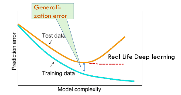
With machine learning models encoding inductive biases, our approach to training them typically consists of two phases: (i) fit the training data; and (ii) estimate the generalization error (the true error on the underlying population) by evaluating the model on holdout data. The difference between our fit on the training data and our fit on the test data is called the generalization gap and when the generalization gap is large, we say that our models overfit to the training data. In extreme cases of overfitting, we might exactly fit the training data, even when the test error remains significant. And in the classical view, the interpretation is that our models are too complex, requiring that we either shrink the number of features, the number of nonzero parameters learned, or the size of the parameters as quantified. Recall the plot of model complexity vs loss (Fig. 3.6.1) from Section 3.6.
3.6. Generalization — Dive into Deep Learning 1.0.0-beta0 documentation
d2l.ai
귀납적 편향을 인코딩하는 기계 학습 모델을 사용하여 학습에 대한 우리의 접근 방식은 일반적으로 두 단계로 구성됩니다. holdout data에 대한 모델을 평가함으로서 (i) 학습 데이터에 적합; (ii) generalization error 예측 (기본 모집단의 실제 오류) 을 수행합니다. 훈련 데이터에 대한 적합도와 테스트 데이터에 대한 적합도의 차이를 일반화 격차(generalization gap)라고 하며, 일반화 격차(generalization gap)가 크면 모델이 훈련 데이터에 과적합되었다고 합니다. 과대적합(overfitting)의 극단적인 경우에는 테스트 오류가 여전히 존재 함에도 training data는 아주 fit할 수도 있습니다. 그리고 고전적 관점에서 해석(interpretation )은 우리 모델이 너무 복잡해서 features 수, 학습된 0이 아닌 매개변수 수 또는 정량화된 매개변수 크기를 축소해야 한다는 것입니다. 섹션 3.6의 모델 복잡성 대 손실 플롯(그림 3.6.1)을 상기하십시오.
However deep learning complicates this picture in counterintuitive ways. First, for classification problems, our models are typically expressive enough to perfectly fit every training example, even in datasets consisting of millions (Zhang et al., 2021). In the classical picture, we might think that this setting lies on the far right extreme of the model complexity axis, and that any improvements in generalization error must come by way of regularization, either by reducing the complexity of the model class, or by applying a penalty, severely constraining the set of values that our parameters might take. But that is where things start to get weird.
그러나 딥 러닝은 직관에 반하는 방식으로 이 그림을 복잡하게 만듭니다. 첫째, 분류 문제의 경우 우리 모델은 일반적으로 수백만 개로 구성된 데이터 세트에서도 모든 교육 예제에 완벽하게 맞을 만큼 표현력이 풍부합니다(Zhang et al., 2021). 고전적인 그림에서 우리는 이 설정이 모델 복잡성 축의 맨 오른쪽 극단에 있으며 일반화 오류의 개선은 모델 클래스의 복잡성을 줄이거나 적용하여 정규화를 통해 이루어져야 한다고 생각할 수 있습니다. 매개변수가 취할 수 있는 값 세트를 심각하게 제한하는 페널티입니다. 그러나 그것은 상황이 이상해지기 시작하는 곳입니다.
Strangely, for many deep learning tasks (e.g., image recognition and text classification) we are typically choosing among model architectures, all of which can achieve arbitrarily low training loss (and zero training error). Because all models under consideration achieve zero training error, the only avenue for further gains is to reduce overfitting. Even stranger, it is often the case that despite fitting the training data perfectly, we can actually reduce the generalization error further by making the model even more expressive, e.g., adding layers, nodes, or training for a larger number of epochs. Stranger yet, the pattern relating the generalization gap to the complexity of the model (as captured, e.g., in the depth or width of the networks) can be non-monotonic, with greater complexity hurting at first but subsequently helping in a so-called “double-descent” pattern (Nakkiran et al., 2021). Thus the deep learning practitioner possesses a bag of tricks, some of which seemingly restrict the model in some fashion and others that seemingly make it even more expressive, and all of which, in some sense, are applied to mitigate overfitting.
이상하게도 많은 딥 러닝 작업(예: 이미지 인식 및 텍스트 분류)의 경우 일반적으로 모델 아키텍처 중에서 선택하며, 모두 임의로 낮은 학습 손실(및 학습 오류 없음)을 달성할 수 있습니다. 고려 중인 모든 모델이 제로 훈련 오류를 달성하기 때문에 추가 이득을 얻을 수 있는 유일한 방법은 과적합을 줄이는 것입니다. 이상하게도 훈련 데이터를 완벽하게 피팅했음에도 불구하고 모델을 훨씬 더 표현력 있게 만들면(예: 계층, 노드 추가 또는 더 많은 에포크에 대한 훈련) 실제로 일반화 오류를 더 줄일 수 있는 경우가 종종 있습니다. 더 이상하게도 모델의 복잡성에 대한 일반화 격차와 관련된 패턴(예: 네트워크의 깊이 또는 너비에서 캡처됨)은 비단조적일 수 있습니다. "이중 하강" 패턴(Nakkiran et al., 2021). 따라서 딥 러닝 실무자는 트릭 가방을 소유하고 있으며, 그 중 일부는 일부 방식으로 모델을 제한하는 것처럼 보이고 다른 일부는 모델을 더욱 표현력있게 만드는 것처럼 보이며 어떤 의미에서 모두 과적합을 완화하는 데 적용됩니다.
Complicating things even further, while the guarantees provided by classical learning theory can be conservative even for classical models, they appear powerless to explain why it is that deep neural networks generalize in the first place. Because deep neural networks are capable of fitting arbitrary labels even for large datasets, and despite the use of familiar methods like ℓ2 regularization, traditional complexity-based generalization bounds, e.g., those based on the VC dimension or Rademacher complexity of a hypothesis class cannot explain why neural networks generalize.
상황을 더욱 복잡하게 만드는 것은 고전적 학습 이론이 제공하는 보장이 고전적 모델에 대해서도 보수적일 수 있지만 심층 신경망이 애초에 일반화되는 이유를 설명하는 데는 무력해 보입니다. 심층 신경망은 대규모 데이터 세트에 대해서도 임의의 레이블을 맞출 수 있고 ℓ2 정규화와 같은 친숙한 방법을 사용함에도 불구하고 기존의 복잡성 기반 일반화 경계를 사용할 수 있기 때문입니다. 예를 들어 VC 차원 또는 가설 클래스의 Rademacher 복잡성을 기반으로 하는 것은 신경망이 일반화되는 이유를 설명할 수 없습니다.
5.5.2. Inspiration from Nonparametrics
Approaching deep learning for the first time, it is tempting to think of them as parametric models. After all, the models do have millions of parameters. When we update the models, we update their parameters. When we save the models, we write their parameters to disk. However, mathematics and computer science are riddled with counterintuitive changes of perspective, and surprising isomorphisms seemingly different problems. While neural networks, clearly have parameters, in some ways, it can be more fruitful to think of them as behaving like nonparametric models. So what precisely makes a model nonparametric? While the name covers a diverse set of approaches, one common theme is that nonparametric methods tend to have a level of complexity that grows as the amount of available data grows.
처음으로 딥 러닝에 접근하면 파라메트릭 모델로 생각하고 싶을 것입니다. 결국 모델에는 수백만 개의 매개변수가 있습니다. 모델을 업데이트하면 매개변수도 업데이트됩니다. 모델을 저장할 때 매개변수를 디스크에 기록합니다. 그러나 수학과 컴퓨터 과학은 직관에 반하는 관점의 변화와 겉보기에 다른 문제로 보이는 놀라운 동형사상으로 가득 차 있습니다. 신경망에는 분명히 매개변수가 있지만 어떤 면에서는 비모수적 모델처럼 작동한다고 생각하는 것이 더 유익할 수 있습니다. 그렇다면 모델을 비모수적으로 만드는 것은 정확히 무엇입니까? 이름은 다양한 접근 방식을 포함하지만 한 가지 공통된 주제는 비모수적 방법이 사용 가능한 데이터의 양이 증가함에 따라 복잡성 수준이 증가하는 경향이 있다는 것입니다.
Parametric이란?
A parametric model is a type of statistical model that assumes a specific functional form or structure with a fixed number of parameters. These parameters represent the underlying characteristics or properties of the model and are estimated from the available data. Once the parameters are determined, the model can make predictions or generate new data points based on the learned relationships between the input variables and the target variable.
모수적 모델은 고정된 수의 파라미터를 가진 특정한 함수 형태나 구조를 가정하는 통계 모델의 유형입니다. 이러한 파라미터는 모델의 기저 특성이나 속성을 나타내며, 이용 가능한 데이터에서 추정됩니다. 파라미터가 결정된 후에는 입력 변수와 목표 변수 사이의 학습된 관계를 기반으로 모델이 예측을 수행하거나 새로운 데이터 포인트를 생성할 수 있습니다.
Parametric models make strong assumptions about the underlying data distribution and the relationship between variables. Examples of parametric models include linear regression, logistic regression, and Gaussian Naive Bayes. These models are often simpler and more interpretable compared to non-parametric models but may have limitations in their flexibility to capture complex patterns in the data.
모수적 모델은 기본 데이터 분포와 변수 간의 관계에 대해 강력한 가정을 가집니다. 선형 회귀, 로지스틱 회귀, 가우시안 나이브 베이즈 등이 모수적 모델의 예입니다. 이러한 모델은 비모수적 모델에 비해 간단하고 해석하기 쉽지만, 데이터에서 복잡한 패턴을 포착하는 데 있어서 유연성이 제한될 수 있습니다.
isomorphizm이란?
Isomorphism refers to a mathematical concept that describes a structural similarity or equivalence between two objects or systems. In the context of mathematics, isomorphism identifies when two mathematical structures can be mapped onto each other in a way that preserves their essential properties and relationships.
동형성은 두 개체 또는 시스템 간의 구조적 유사성이나 동등성을 설명하는 수학적 개념입니다. 수학의 맥락에서 동형성은 두 개의 수학적 구조가 서로 대응되어 그들의 본질적인 특성과 관계를 보존하는 방식으로 매핑될 수 있을 때 나타납니다.
In simple terms, isomorphism means that two objects or systems have the same underlying structure, even though they may appear different or have different representations. It implies that the objects or systems have the same fundamental characteristics and can be considered equivalent in terms of their structure.
간단히 말하면, 동형성은 두 개체나 시스템이 동일한 기본 구조를 가지고 있음을 의미합니다. 이들은 서로 다른 모습이거나 다른 표현을 가질 수 있지만, 핵심적인 특성과 구조에서는 동등하다고 볼 수 있습니다.
For example, in graph theory, two graphs are isomorphic if they have the same number of vertices and edges, and the arrangement of these vertices and edges can be matched. Similarly, in abstract algebra, groups or vector spaces are considered isomorphic if they exhibit the same algebraic structure and operations.
예를 들어, 그래프 이론에서 두 개의 그래프가 동형이라면 그들은 동일한 개수의 정점과 간선을 가지며, 이러한 정점과 간선의 배열을 일치시킬 수 있습니다. 마찬가지로, 추상 대수학에서는 그룹이나 벡터 공간이 동형적으로 간주됩니다만, 이는 동일한 대수적 구조와 연산을 나타내기 때문입니다.
Nonparametric model이란?
A nonparametric model is a type of statistical or machine learning model that does not make explicit assumptions about the functional form or distribution of the data. Unlike parametric models, which have a fixed number of parameters and assume a specific functional form, nonparametric models are more flexible and can adapt to various types of data distributions. They are often used when the underlying data distribution is unknown or when there is no clear assumption about the relationship between the input and output variables. Nonparametric models rely on data-driven techniques to estimate the relationship or pattern in the data, allowing them to capture complex patterns and relationships without making strong assumptions.
비모수 모델은 통계 또는 기계 학습 모델의 한 유형으로, 데이터의 함수 형태나 분포에 대한 명시적인 가정을 하지 않는 모델입니다. 비모수 모델은 고정된 수의 파라미터와 특정한 함수 형태를 가정하는 모수적 모델과 달리, 유연성이 높으며 다양한 유형의 데이터 분포에 적응할 수 있습니다. 이러한 모델은 기초 데이터 분포가 알려지지 않았거나 입력과 출력 변수 간의 관계에 대한 명확한 가정이 없을 때 주로 사용됩니다. 비모수 모델은 데이터 기반 기법을 사용하여 데이터 내의 관계나 패턴을 추정하며, 강력한 가정을 하지 않고도 복잡한 패턴과 관계를 포착할 수 있습니다.
K-nearest neighbor algorithm이란?
The k-nearest neighbor (KNN) algorithm is a type of supervised learning algorithm used for both classification and regression tasks. It is a non-parametric algorithm, meaning it does not make any assumptions about the underlying data distribution. KNN is a lazy learning algorithm, which means that it does not explicitly build a model during the training phase. Instead, it memorizes the entire training dataset and makes predictions by finding the k nearest neighbors to a given query point in the feature space. The prediction is based on the majority vote (for classification) or the average (for regression) of the labels or values of the k nearest neighbors. The choice of k determines the level of flexibility and generalization of the algorithm.
k-최근접 이웃 (K-nearest neighbor, KNN) 알고리즘은 분류 및 회귀 작업에 사용되는 지도 학습 알고리즘입니다. 이 알고리즘은 비모수적인 알고리즘으로, 기반이 되는 데이터 분포에 대한 가정을 하지 않습니다. KNN은 레이지 학습 알고리즘으로, 훈련 단계에서 명시적으로 모델을 구축하지 않습니다. 대신, 특징 공간에서 주어진 쿼리 지점에 대해 k개의 최근접 이웃을 찾아 예측을 수행합니다. 분류 작업에서는 k개의 최근접 이웃의 레이블 중 가장 많은 레이블을 예측값으로 선택하고, 회귀 작업에서는 k개의 최근접 이웃의 값들의 평균을 예측값으로 사용합니다. k의 선택은 알고리즘의 유연성과 일반화 수준을 결정합니다.
Perhaps the simplest example of a nonparametric model is the k-nearest neighbor algorithm (we will cover more nonparametric models later, such as in Section 11.2). Here, at training time, the learner simply memorizes the dataset. Then, at prediction time, when confronted with a new point x, the learner looks up the k nearest neighbors (the x points x′i that minimize some distance d(x,x′i)). When k=1, this is algorithm is called 1-nearest neighbors, and the algorithm will always achieve a training error of zero. That however, does not mean that the algorithm will not generalize. In fact, it turns out that under some mild conditions, the 1-nearest neighbor algorithm is consistent (eventually converging to the optimal predictor).
아마도 비모수적 모델의 가장 간단한 예는 k-최근접 이웃 알고리즘일 것입니다(섹션 11.2와 같이 나중에 더 많은 비모수적 모델을 다룰 것입니다). 여기서 훈련 시간에 학습자는 단순히 데이터 세트를 기억합니다. 그런 다음 예측 시간에 새로운 점 x와 마주쳤을 때 학습자는 k개의 가장 가까운 이웃을 찾습니다(어떤 거리 d(x,x′i)를 최소화하는 x 점 x′i). k=1일 때, 이 알고리즘은 1-최근접 이웃이라고 하며 알고리즘은 항상 0의 학습 오류를 달성합니다. 그러나 알고리즘이 일반화되지 않는다는 의미는 아닙니다. 실제로 일부 온화한 조건에서 1-최근접 이웃 알고리즘이 일관됨이 밝혀졌습니다(결국 최적의 예측 변수로 수렴).
Note that 1 nearest neighbor requires that we specify some distance function d, or equivalently, that we specify some vector-valued basis function φ(x) for featurizing our data. For any choice of the distance metric, we will achieve 0 training error and eventually reach an optimal predictor, but different distance metrics d encode different inductive biases and with a finite amount of available data will yield different predictors. Different choices of the distance metric d represent different assumptions about the underlying patterns and the performance of the different predictors will depend on how compatible the assumptions are with the observed data.
1개의 가장 가까운 이웃은 거리 함수 d를 지정하거나 이와 동등하게 데이터를 특성화하기 위해 일부 벡터 값 기본 함수 φ(x)를 지정해야 합니다. 어떤 거리 메트릭을 선택하든 훈련 오류가 0이 되고 결국 최적의 예측 변수에 도달하지만 다른 거리 메트릭은 다른 유도 편향을 인코딩하고 한정된 양의 사용 가능한 데이터로 다른 예측 변수를 생성합니다. 거리 메트릭 d의 다른 선택은 기본 패턴에 대한 다른 가정을 나타내며 다른 예측자의 성능은 가정이 관찰된 데이터와 얼마나 호환되는지에 따라 달라집니다.
In a sense, because neural networks are over-parameterized, possessing many more parameters than are needed to fit the training data, they tend to interpolate the training data (fitting it perfectly) and thus behave, in some ways, more like nonparametric models. More recent theoretical research has established deep connection between large neural networks and nonparametric methods, notably kernel methods. In particular, Jacot et al. (2018) demonstrated that in the limit, as multilayer perceptrons with randomly initialized weights grow infinitely wide, they become equivalent to (nonparametric) kernel methods for a specific choice of the kernel function (essentially, a distance function), which they call the neural tangent kernel. While current neural tangent kernel models may not fully explain the behavior of modern deep networks, their success as an analytical tool underscores the usefulness of nonparametric modeling for understanding the behavior of over-parameterized deep networks.
어떤 의미에서 신경망은 훈련 데이터에 맞추는 데 필요한 것보다 더 많은 매개변수를 가지고 있는 과잉 매개변수화되기 때문에 훈련 데이터를 보간(완벽하게 맞추는) 경향이 있으므로 어떤 면에서는 비모수적 모델처럼 작동합니다. 보다 최근의 이론적 연구는 대규모 신경망과 비모수적 방법, 특히 커널 방법 사이에 깊은 연관성을 확립했습니다. 특히 Jacot et al. (2018)은 극한에서 무작위로 초기화된 가중치가 있는 다층 퍼셉트론이 무한히 넓어짐에 따라 커널 함수(본질적으로 거리 함수)의 특정 선택에 대한 (비모수적) 커널 방법과 동등해진다는 것을 보여주었습니다. 탄젠트 커널. 현재의 뉴럴 탄젠트 커널 모델은 최신 심층 네트워크의 동작을 완전히 설명하지 못할 수 있지만 분석 도구로서의 성공은 과도하게 매개변수화된 심층 네트워크의 동작을 이해하기 위한 비모수적 모델링의 유용성을 강조합니다.
5.5.3. Early Stopping
While deep neural networks are capable of fitting arbitrary labels, even when labels are assigned incorrectly or randomly (Zhang et al., 2021), this ability only emerges over many iterations of training. A new line of work (Rolnick et al., 2017) has revealed that in the setting of label noise, neural networks tend to fit cleanly labeled data first and only subsequently to interpolate the mislabeled data. Moreover, it is been established that this phenomenon translates directly into a guarantee on generalization: whenever a model has fitted the cleanly labeled data but not randomly labeled examples included in the training set, it has in fact generalized (Garg et al., 2021).
심층 신경망은 임의의 레이블을 맞출 수 있지만 레이블이 잘못되거나 무작위로 할당된 경우에도(Zhang et al., 2021) 이 능력은 많은 반복 훈련을 통해서만 나타납니다. 새로운 작업 라인(Rolnick et al., 2017)은 레이블 노이즈 설정에서 신경망이 처음에는 깔끔하게 레이블이 지정된 데이터를 맞춘 다음 잘못 레이블이 지정된 데이터를 보간하는 경향이 있음을 밝혔습니다. 또한, 이 현상은 일반화에 대한 보장으로 직접 변환된다는 것이 입증되었습니다. 모델이 훈련 세트에 포함된 무작위로 레이블이 지정된 예가 아닌 깔끔하게 레이블이 지정된 데이터를 적합할 때마다 실제로 일반화되었습니다(Garg et al., 2021). .
Together these findings help to motivate early stopping, a classic technique for regularizing deep neural networks. Here, rather than directly constraining the values of the weights, one constrains the number of epochs of training. The most common way to determine the stopping criteria is to monitor validation error throughout training (typically by checking once after each epoch) and to cut off training when the validation error has not decreased by more than some small amount ϵ for some number of epochs. This is sometimes called a patience criteria. Besides the potential to lead to better generalization, in the setting of noisy labels, another benefit of early stopping is the time saved. Once the patience criteria is met, one can terminate training. For large models that might require days of training simultaneously across 8 GPUs or more, well-tuned early stopping can save researchers days of time and can save their employers many thousands of dollars.
이와함께 이러한 발견은 심층 신경망을 정규화하기 위한 고전적인 기술인 조기 중지에 동기를 부여하는 데 도움이 됩니다. 여기서는 가중치 값을 직접적으로 제한하는 대신 학습 에포크 수를 제한합니다. 중지 기준을 결정하는 가장 일반적인 방법은 훈련 전반에 걸쳐 유효성 검사 오류를 모니터링하고(일반적으로 각 에포크 후 한 번 확인) 유효성 검사 오류가 일부 에포크 동안 소량 ϵ 이상 감소하지 않으면 교육을 중단하는 것입니다. 이를 인내 기준이라고도 합니다. 더 나은 일반화로 이어질 수 있는 가능성 외에도 노이즈 레이블 설정에서 조기 중지의 또 다른 이점은 시간 절약입니다. 인내심 기준이 충족되면 교육을 종료할 수 있습니다. 8개 이상의 GPU에서 동시에 며칠 동안 훈련해야 할 수 있는 대규모 모델의 경우 잘 조정된 조기 중단을 통해 연구원은 며칠의 시간을 절약하고 고용주는 수천 달러를 절약할 수 있습니다.
Notably, when there is no label noise and datasets are realizable (the classes are truly separable, e.g., distinguishing cats from dogs), early stopping tends not to lead to significant improvements in generalization. On the other hand, when there is label noise, or intrinsic variability in the label (e.g., predicting mortality among patients), early stopping is crucial. Training models until they interpolate noisy data is typically a bad idea.
특히 레이블 노이즈가 없고 데이터 세트를 실현할 수 있는 경우(예: 고양이와 개를 구별하는 등 클래스가 진정으로 분리 가능함) 조기 중지는 일반화에서 상당한 개선으로 이어지지 않는 경향이 있습니다. 반면에 라벨에 노이즈가 있거나 라벨에 본질적인 가변성이 있는 경우(예: 환자의 사망률 예측) 조기 중단이 중요합니다. 시끄러운 데이터를 보간할 때까지 모델을 교육하는 것은 일반적으로 나쁜 생각입니다.
5.5.4. Classical Regularization Methods for Deep Networks
In Section 3, we described several classical regularization techniques for constraining the complexity of our models. In particular, Section 3.7 introduced a method called weight decay, which consists of adding a regularization term to the loss function to penalize large values of the weights. Depending on which weight norm is penalized this technique is known either as ridge regularization (for ℓ2 penalty) or lasso regularization (for an ℓ1 penalty). In the classical analysis of these regularizers, they are considered to restrict the values that the weights can take sufficiently to prevent the model from fitting arbitrary labels.
섹션 3에서 모델의 복잡성을 제한하기 위한 몇 가지 고전적인 정규화 기술을 설명했습니다. 특히 3.7절에서는 가중치 감쇠라는 방법을 소개했는데, 이 방법은 손실 함수에 정규화 항을 추가하여 큰 가중치 값에 페널티를 부여하는 것으로 구성됩니다. 어떤 가중치 규범에 불이익이 있는지에 따라 이 기술은 능선 정규화(ℓ2 벌점) 또는 올가미 정규화(ℓ1 불이익)로 알려져 있습니다. 이러한 regularizer의 고전적 분석에서는 모델이 임의의 레이블을 맞추지 못하도록 가중치가 충분히 취할 수 있는 값을 제한하는 것으로 간주됩니다.
In deep learning implementations, weight decay remains a popular tool. However, researchers have noted that typical strengths of ℓ2 regularization are insufficient to prevent the networks from interpolating the data (Zhang et al., 2021) and thus the benefits if interpreted as regularization might only make sense in combination with the early stopping criteria. Absent early stopping, it is possible that just like the number of layers or number of nodes (in deep learning) or the distance metric (in 1-nearest neighbor), these methods may lead to better generalization not because they meaningfully constrain the power of the neural network but rather because they somehow encode inductive biases that are better compatible with the patterns found in datasets of interests. Thus, classical regularizers remain popular in deep learning implementations, even if the theoretical rationale for their efficacy may be radically different.
딥 러닝 구현에서 가중치 감소는 여전히 널리 사용되는 도구입니다. 그러나 연구원들은 ℓ2 정규화의 일반적인 강점이 네트워크가 데이터를 보간하는 것을 방지하기에 불충분하므로(Zhang et al., 2021) 정규화로 해석되는 경우 이점은 조기 중지 기준과 함께만 의미가 있을 수 있다고 지적했습니다. 초기 중지가 없으면 레이어 수 또는 노드 수(딥 러닝에서) 또는 거리 메트릭(1-가장 가까운 이웃에서)과 마찬가지로 이러한 방법이 의미 있는 힘을 제한하기 때문이 아니라 더 나은 일반화로 이어질 수 있습니다. 관심 있는 데이터 세트에서 발견된 패턴과 더 잘 호환되는 귀납적 편향을 어떻게든 인코딩하기 때문입니다. 따라서 고전적 정규화기는 효능에 대한 이론적 근거가 근본적으로 다를 수 있지만 딥 러닝 구현에서 여전히 인기가 있습니다.
Notably, deep learning researchers have also built on techniques first popularized in classical regularization contexts, such as adding noise to model inputs. In the next section we will introduce the famous dropout technique (invented by Srivastava et al. (2014)), which has become a mainstay of deep learning, even as the theoretical basis for its efficacy remains similarly mysterious.
특히 딥 러닝 연구자들은 모델 입력에 노이즈를 추가하는 것과 같이 고전적인 정규화 맥락에서 처음으로 대중화된 기술을 기반으로 구축했습니다. 다음 섹션에서는 효능에 대한 이론적 근거가 유사하게 미스터리로 남아 있음에도 불구하고 딥 러닝의 주류가 된 유명한 드롭아웃 기술(Srivastava et al.(2014)이 발명)을 소개합니다.
5.5.5. Summary
Unlike classical linear models, which tend to have fewer parameters than examples, deep networks tend to be over-parameterized, and for most tasks are capable of perfectly fitting the training set. This interpolation regime challenges many of hard fast-held intuitions. Functionally, neural networks look like parametric models. But thinking of them as nonparametric models can sometimes be a more reliable source of intuition. Because it is often the case that all deep networks under consideration are capable of fitting all of the training labels, nearly all gains must come by mitigating overfitting (closing the generalization gap). Paradoxically, the interventions that reduce the generalization gap sometimes appear to increase model complexity and at other times appear to decrease complexity. However, these methods seldom decrease complexity sufficiently for classical theory to explain the generalization of deep networks, and why certain choices lead to improved generalization remains for the most part a massive open question despite the concerted efforts of many brilliant researchers.
예보다 매개변수가 적은 기존 선형 모델과 달리 딥 네트워크는 매개변수가 과도하게 지정되는 경향이 있으며 대부분의 작업에서 훈련 세트를 완벽하게 맞출 수 있습니다. 이 보간 방식은 많은 고정된 직관에 도전합니다. 기능적으로 신경망은 파라메트릭 모델처럼 보입니다. 그러나 그것들을 비모수적 모델로 생각하는 것이 때때로 더 신뢰할 수 있는 직관의 원천이 될 수 있습니다. 고려 중인 모든 딥 네트워크가 모든 훈련 레이블을 맞출 수 있는 경우가 많기 때문에 거의 모든 이득은 과대적합을 완화(일반화 격차를 줄이는 것)해야 합니다. 역설적이게도 일반화 격차를 줄이는 개입은 때때로 모델 복잡성을 증가시키는 것처럼 보이고 다른 경우에는 복잡성을 감소시키는 것처럼 보입니다. 그러나 이러한 방법은 고전 이론이 심층 네트워크의 일반화를 설명할 수 있을 만큼 충분히 복잡성을 줄이는 경우가 거의 없으며, 특정 선택이 개선된 일반화로 이어지는 이유는 많은 훌륭한 연구자들의 공동 노력에도 불구하고 대부분의 경우 방대한 미해결 질문으로 남아 있습니다.
5.5.6. Exercises
- In what sense do traditional complexity-based measures fail to account for generalization of deep neural networks?
- Why might early stopping be considered a regularization technique?
- How do researchers typically determine the stopping criteria?
- What important factor seems to differentiate cases when early stopping leads to big improvements in generalization?
- Beyond generalization, describe another benefit of early stopping.
'Dive into Deep Learning > D2L Multilayer Perceptrons Builder Guide' 카테고리의 다른 글
| D2L - 5.7. Predicting House Prices on Kaggle (0) | 2023.07.03 |
|---|---|
| D2L - 5.6. Dropout (0) | 2023.07.03 |
| D2L - 5.4. Numerical Stability and Initialization (0) | 2023.07.02 |
| D2L - 5.3. Forward Propagation, Backward Propagation, and Computational Graphs (0) | 2023.07.02 |
| D2L - 5.2. Implementation of Multilayer Perceptrons (0) | 2023.07.01 |
| D2L - 5.1. Multilayer Perceptrons (0) | 2023.07.01 |
| D2L - 5. Multilayer Perceptrons (1) | 2023.06.30 |