
https://d2l.ai/chapter_hyperparameter-optimization/hyperopt-intro.html
19.1. What Is Hyperparameter Optimization? — Dive into Deep Learning 1.0.3 documentation
d2l.ai
19.1. What Is Hyperparameter Optimization?
As we have seen in the previous chapters, deep neural networks come with a large number of parameters or weights that are learned during training. On top of these, every neural network has additional hyperparameters that need to be configured by the user. For example, to ensure that stochastic gradient descent converges to a local optimum of the training loss (see Section 12), we have to adjust the learning rate and batch size. To avoid overfitting on training datasets, we might have to set regularization parameters, such as weight decay (see Section 3.7) or dropout (see Section 5.6). We can define the capacity and inductive bias of the model by setting the number of layers and number of units or filters per layer (i.e., the effective number of weights).
이전 장에서 살펴본 것처럼 심층 신경망에는 훈련 중에 학습되는 수많은 매개변수 또는 가중치가 포함됩니다. 게다가 모든 신경망에는 사용자가 구성해야 하는 추가 하이퍼파라미터가 있습니다. 예를 들어 확률적 경사하강법이 훈련 손실의 국소 최적값으로 수렴되도록 하려면(섹션 12 참조) 학습 속도와 배치 크기를 조정해야 합니다. 훈련 데이터세트에 대한 과적합을 방지하려면 가중치 감소(섹션 3.7 참조) 또는 드롭아웃(섹션 5.6 참조)과 같은 정규화 매개변수를 설정해야 할 수도 있습니다. 레이어 수와 레이어당 단위 또는 필터 수(즉, 유효 가중치 수)를 설정하여 모델의 용량과 유도 편향을 정의할 수 있습니다.
Unfortunately, we cannot simply adjust these hyperparameters by minimizing the training loss, because this would lead to overfitting on the training data. For example, setting regularization parameters, such as dropout or weight decay to zero leads to a small training loss, but might hurt the generalization performance.
불행하게도 훈련 손실을 최소화함으로써 이러한 하이퍼파라미터를 간단히 조정할 수는 없습니다. 왜냐하면 그렇게 하면 훈련 데이터에 과적합이 발생할 수 있기 때문입니다. 예를 들어, 드롭아웃이나 가중치 감소와 같은 정규화 매개변수를 0으로 설정하면 훈련 손실이 약간 발생하지만 일반화 성능이 저하될 수 있습니다.
Without a different form of automation, hyperparameters have to be set manually in a trial-and-error fashion, in what amounts to a time-consuming and difficult part of machine learning workflows. For example, consider training a ResNet (see Section 8.6) on CIFAR-10, which requires more than 2 hours on an Amazon Elastic Cloud Compute (EC2) g4dn.xlarge instance. Even just trying ten hyperparameter configurations in sequence, this would already take us roughly one day. To make matters worse, hyperparameters are usually not directly transferable across architectures and datasets (Bardenet et al., 2013, Feurer et al., 2022, Wistuba et al., 2018), and need to be re-optimized for every new task. Also, for most hyperparameters, there are no rule-of-thumbs, and expert knowledge is required to find sensible values.
다른 형태의 자동화가 없으면 하이퍼파라미터는 시행착오 방식으로 수동으로 설정해야 하므로 기계 학습 워크플로에서 시간이 많이 걸리고 어려운 부분이 됩니다. 예를 들어, Amazon Elastic Cloud Compute(EC2) g4dn.xlarge 인스턴스에서 2시간 이상 필요한 CIFAR-10의 ResNet(섹션 8.6 참조) 교육을 고려해 보세요. 10개의 하이퍼파라미터 구성을 순차적으로 시도하는 것만으로도 이미 대략 하루가 걸릴 것입니다. 설상가상으로 하이퍼파라미터는 일반적으로 아키텍처와 데이터 세트 간에 직접 전송할 수 없으며(Bardenet et al., 2013, Feurer et al., 2022, Wistuba et al., 2018) 모든 새로운 작업에 대해 다시 최적화해야 합니다. 또한 대부분의 하이퍼파라미터에는 경험 법칙이 없으며, 합리적인 값을 찾기 위해서는 전문 지식이 필요합니다.
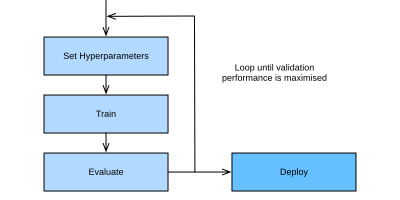
Hyperparameter optimization (HPO) algorithms are designed to tackle this problem in a principled and automated fashion (Feurer and Hutter, 2018), by framing it as a global optimization problem. The default objective is the error on a hold-out validation dataset, but could in principle be any other business metric. It can be combined with or constrained by secondary objectives, such as training time, inference time, or model complexity.
하이퍼파라미터 최적화(HPO) 알고리즘은 이 문제를 전역 최적화 문제로 구성하여 원칙적이고 자동화된 방식으로(Feurer and Hutter, 2018) 해결하도록 설계되었습니다. 기본 목표는 홀드아웃 검증 데이터 세트의 오류이지만 원칙적으로 다른 비즈니스 지표일 수도 있습니다. 이는 훈련 시간, 추론 시간 또는 모델 복잡성과 같은 2차 목표와 결합되거나 제한될 수 있습니다.
Recently, hyperparameter optimization has been extended to neural architecture search (NAS) (Elsken et al., 2018, Wistuba et al., 2019), where the goal is to find entirely new neural network architectures. Compared to classical HPO, NAS is even more expensive in terms of computation and requires additional efforts to remain feasible in practice. Both, HPO and NAS can be considered as sub-fields of AutoML (Hutter et al., 2019), which aims to automate the entire ML pipeline.
최근 하이퍼파라미터 최적화는 완전히 새로운 신경망 아키텍처를 찾는 것이 목표인 신경 아키텍처 검색(NAS)(Elsken et al., 2018, Wistuba et al., 2019)으로 확장되었습니다. 기존 HPO에 비해 NAS는 계산 측면에서 훨씬 더 비싸며 실제로 실행 가능성을 유지하려면 추가 노력이 필요합니다. HPO와 NAS는 모두 전체 ML 파이프라인 자동화를 목표로 하는 AutoML(Hutter et al., 2019)의 하위 분야로 간주될 수 있습니다.
In this section we will introduce HPO and show how we can automatically find the best hyperparameters of the logistic regression example introduced in Section 4.5.
이 섹션에서는 HPO를 소개하고 섹션 4.5에 소개된 로지스틱 회귀 예제의 최상의 하이퍼파라미터를 자동으로 찾는 방법을 보여줍니다.
19.1.1. The Optimization Problem
We will start with a simple toy problem: searching for the learning rate of the multi-class logistic regression model SoftmaxRegression from Section 4.5 to minimize the validation error on the Fashion MNIST dataset. While other hyperparameters like batch size or number of epochs are also worth tuning, we focus on learning rate alone for simplicity.
간단한 장난감 문제부터 시작하겠습니다. Fashion MNIST 데이터세트의 검증 오류를 최소화하기 위해 섹션 4.5에서 다중 클래스 로지스틱 회귀 모델 SoftmaxRegression의 학습률을 검색하는 것입니다. 배치 크기나 에포크 수와 같은 다른 하이퍼파라미터도 조정할 가치가 있지만 단순화를 위해 학습 속도에만 중점을 둡니다.
import numpy as np
import torch
from scipy import stats
from torch import nn
from d2l import torch as d2l
Before we can run HPO, we first need to define two ingredients: the objective function and the configuration space.
HPO를 실행하기 전에 먼저 목적 함수와 구성 공간이라는 두 가지 구성 요소를 정의해야 합니다.
19.1.1.1. The Objective Function
The performance of a learning algorithm can be seen as a function f:X→ℝ that maps from the hyperparameter space x∈D to the validation loss. For every evaluation of f(x), we have to train and validate our machine learning model, which can be time and compute intensive in the case of deep neural networks trained on large datasets. Given our criterion f(x) our goal is to find x⋆∈argminx∈Xf(x).
학습 알고리즘의 성능은 하이퍼파라미터 공간 x∈D에서 검증 손실로 매핑되는 함수 f:X→ℝ로 볼 수 있습니다. f(x)를 평가할 때마다 기계 학습 모델을 훈련하고 검증해야 하는데, 이는 대규모 데이터 세트에 대해 훈련된 심층 신경망의 경우 시간과 계산 집약적일 수 있습니다. 기준 f(x)가 주어지면 우리의 목표는 x⋆∈argminx∈Xf(x)를 찾는 것입니다.
There is no simple way to compute gradients of f with respect to x, because it would require to propagate the gradient through the entire training process. While there is recent work (Franceschi et al., 2017, Maclaurin et al., 2015) to drive HPO by approximate “hypergradients”, none of the existing approaches are competitive with the state-of-the-art yet, and we will not discuss them here. Furthermore, the computational burden of evaluating f requires HPO algorithms to approach the global optimum with as few samples as possible.
x에 대한 f의 기울기를 계산하는 간단한 방법은 없습니다. 왜냐하면 전체 훈련 과정을 통해 기울기를 전파해야 하기 때문입니다. 대략적인 "hypergradients"를 통해 HPO를 구동하는 최근 연구(Franceschi et al., 2017, Maclaurin et al., 2015)가 있지만 기존 접근 방식 중 어느 것도 아직 최첨단 기술과 경쟁할 수 없습니다. 여기서는 논의하지 마세요. 더욱이, f를 평가하는 계산 부담으로 인해 HPO 알고리즘은 가능한 적은 샘플을 사용하여 전역 최적에 접근해야 합니다.
The training of neural networks is stochastic (e.g., weights are randomly initialized, mini-batches are randomly sampled), so that our observations will be noisy: y∼f(x)+ϵ, where we usually assume that the ϵ∼N(0,σ) observation noise is Gaussian distributed.
신경망의 훈련은 확률론적입니다(예: 가중치는 무작위로 초기화되고, 미니 배치는 무작위로 샘플링됩니다). 따라서 우리의 관측값은 시끄러울 것입니다: y∼f(x)+ϵ, 여기서 우리는 일반적으로 ϵ∼N( 0,σ) 관측 잡음은 가우스 분포입니다.
Faced with all these challenges, we usually try to identify a small set of well performing hyperparameter configurations quickly, instead of hitting the global optima exactly. However, due to large computational demands of most neural networks models, even this can take days or weeks of compute. We will explore in Section 19.4 how we can speed-up the optimization process by either distributing the search or using cheaper-to-evaluate approximations of the objective function.
이러한 모든 문제에 직면했을 때 우리는 일반적으로 전체 최적 상태에 정확히 도달하는 대신 성능이 좋은 소수의 하이퍼파라미터 구성 세트를 신속하게 식별하려고 노력합니다. 그러나 대부분의 신경망 모델의 컴퓨팅 요구량이 많기 때문에 이 작업에도 며칠 또는 몇 주가 걸릴 수 있습니다. 우리는 섹션 19.4에서 검색을 분산하거나 목적 함수의 평가 비용이 더 저렴한 근사치를 사용하여 최적화 프로세스의 속도를 높일 수 있는 방법을 탐색할 것입니다.
We begin with a method for computing the validation error of a model.
모델의 검증 오류를 계산하는 방법부터 시작합니다.
class HPOTrainer(d2l.Trainer):  #@save
    def validation_error(self):
        self.model.eval()
        accuracy = 0
        val_batch_idx = 0
        for batch in self.val_dataloader:
            with torch.no_grad():
                x, y = self.prepare_batch(batch)
                y_hat = self.model(x)
                accuracy += self.model.accuracy(y_hat, y)
            val_batch_idx += 1
        return 1 -  accuracy / val_batch_idx
위의 코드는 하이퍼파라미터 최적화(Hyperparameter Optimization, HPO)를 수행하는 데 사용되는 HPOTrainer 클래스를 정의하는 파트입니다. 코드의 목적과 각 부분에 대한 설명은 다음과 같습니다:
- class HPOTrainer(d2l.Trainer):: HPOTrainer 클래스를 정의합니다. 이 클래스는 d2l.Trainer 클래스를 상속받아 하이퍼파라미터 최적화를 위한 훈련 기능을 추가합니다.
- def validation_error(self):: 검증 데이터셋을 사용하여 모델의 성능을 평가하고 검증 오차를 계산하는 메서드를 정의합니다.
- self.model.eval(): 모델을 평가 모드로 설정합니다. 이 모드에서는 모델이 평가되기만 하고 그라디언트 계산이 비활성화됩니다.
- accuracy = 0: 정확도를 초기화합니다. 이 변수는 모든 검증 배치의 정확도를 누적하기 위해 사용됩니다.
- val_batch_idx = 0: 검증 배치의 인덱스를 초기화합니다.
- for batch in self.val_dataloader:: 검증 데이터셋의 배치들을 반복합니다. self.val_dataloader는 검증 데이터셋을 로드하는 데 사용되는 데이터 로더입니다.
- with torch.no_grad():: 그라디언트 계산을 비활성화하는 torch.no_grad() 컨텍스트를 생성합니다. 이 컨텍스트 내에서는 모델이 평가될 때 그라디언트가 계산되지 않습니다.
- x, y = self.prepare_batch(batch): 현재 배치를 준비하고 입력 데이터 x와 레이블 y를 가져옵니다.
- y_hat = self.model(x): 모델을 사용하여 입력 데이터에 대한 예측을 계산합니다.
- accuracy += self.model.accuracy(y_hat, y): 현재 배치의 정확도를 계산하여 누적합니다. self.model.accuracy()는 모델의 예측과 실제 레이블을 사용하여 정확도를 계산하는 메서드입니다.
- val_batch_idx += 1: 검증 배치 인덱스를 증가시킵니다.
- return 1 - accuracy / val_batch_idx: 검증 데이터셋 전체에 대한 정확도를 계산하고, 1에서 빼서 검증 오차를 계산합니다. 이 오차는 하이퍼파라미터 최적화 과정에서 사용될 수 있습니다.
이렇게 정의된 HPOTrainer 클래스는 모델의 성능을 검증 데이터셋을 사용하여 평가하고 검증 오차를 계산하는 기능을 제공합니다. 이 클래스는 하이퍼파라미터 최적화의 일부로 모델의 성능을 측정하는 데 유용하게 사용될 수 있습니다.
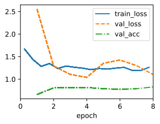
We optimize validation error with respect to the hyperparameter configuration config, consisting of the learning_rate. For each evaluation, we train our model for max_epochs epochs, then compute and return its validation error:
learning_rate로 구성된 하이퍼파라미터 구성 config에 대한 검증 오류를 최적화합니다. 각 평가에 대해 max_epochs epoch에 대한 모델을 훈련한 다음 검증 오류를 계산하고 반환합니다.
def hpo_objective_softmax_classification(config, max_epochs=8):
    learning_rate = config["learning_rate"]
    trainer = d2l.HPOTrainer(max_epochs=max_epochs)
    data = d2l.FashionMNIST(batch_size=16)
    model = d2l.SoftmaxRegression(num_outputs=10, lr=learning_rate)
    trainer.fit(model=model, data=data)
    return trainer.validation_error().detach().numpy()
위의 코드는 하이퍼파라미터 최적화(Hyperparameter Optimization, HPO)를 수행하기 위한 목적 함수인 hpo_objective_softmax_classification를 정의하는 파트입니다. 이 함수는 주어진 하이퍼파라미터 구성을 사용하여 소프트맥스 분류 모델을 훈련하고 검증 오차를 반환합니다. 코드의 목적과 각 부분에 대한 설명은 다음과 같습니다:
- def hpo_objective_softmax_classification(config, max_epochs=8):: 하이퍼파라미터 최적화를 위한 목적 함수를 정의합니다. 함수는 두 개의 매개변수를 입력으로 받습니다. config는 하이퍼파라미터 구성을 나타내며, max_epochs는 모델의 최대 훈련 에폭을 지정하는 매개변수로 기본값은 8입니다.
- learning_rate = config["learning_rate"]: 주어진 하이퍼파라미터 구성에서 학습률(learning rate)을 가져옵니다. 이는 하이퍼파라미터 최적화의 일부로 조정될 값입니다.
- trainer = d2l.HPOTrainer(max_epochs=max_epochs): 하이퍼파라미터 최적화를 위한 d2l.HPOTrainer 객체를 생성합니다. max_epochs는 모델의 최대 훈련 에폭을 설정합니다.
- data = d2l.FashionMNIST(batch_size=16): Fashion MNIST 데이터셋을 로드하고 데이터 로더를 생성합니다. 이 데이터는 모델을 훈련하기 위한 학습 및 검증 데이터로 사용됩니다. batch_size는 한 번에 처리할 데이터의 배치 크기를 설정합니다.
- model = d2l.SoftmaxRegression(num_outputs=10, lr=learning_rate): 소프트맥스 회귀(Softmax Regression) 모델을 생성합니다. num_outputs는 출력 클래스(레이블)의 수를 설정하며, lr은 학습률을 설정합니다.
- trainer.fit(model=model, data=data): trainer를 사용하여 모델을 학습합니다. 모델과 데이터를 전달하고, 지정된 에폭 수(max_epochs)만큼 훈련을 수행합니다.
- return trainer.validation_error().detach().numpy(): 훈련된 모델의 검증 오차를 계산하고 반환합니다. 검증 오차는 trainer.validation_error()를 통해 얻으며, NumPy 배열로 변환하여 반환합니다.
이 함수는 주어진 하이퍼파라미터 구성을 사용하여 모델을 훈련하고 검증 오차를 반환하므로, 하이퍼파라미터 최적화 알고리즘(예: Bayesian Optimization)에 의해 최적의 하이퍼파라미터 구성을 찾는 데 사용됩니다.
19.1.1.2. The Configuration Space
Along with the objective function f(x), we also need to define the feasible set x∈X to optimize over, known as configuration space or search space. For our logistic regression example, we will use:
목적 함수 objective function f(x)와 함께 구성 공간 configuration space 또는 검색 공간 search space 으로 알려진 최적화를 위한 실행 가능한 집합 x∈X도 정의해야 합니다. 로지스틱 회귀 예제에서는 다음을 사용합니다.
config_space = {"learning_rate": stats.loguniform(1e-4, 1)}위의 코드는 하이퍼파라미터 최적화를 위한 하이퍼파라미터 공간을 정의하는 부분입니다. 코드의 목적과 각 부분에 대한 설명은 다음과 같습니다:
- config_space = {"learning_rate": stats.loguniform(1e-4, 1)}: config_space라는 딕셔너리를 정의합니다. 이 딕셔너리는 하이퍼파라미터 공간을 설명하는 엔트리(항목)를 포함합니다.
- "learning_rate": 이 항목은 하이퍼파라미터의 이름인 "learning_rate"를 나타냅니다. 이 이름은 해당 하이퍼파라미터를 식별하는 데 사용됩니다.
- stats.loguniform(1e-4, 1): "learning_rate" 하이퍼파라미터의 값 범위를 지정합니다. stats.loguniform은 로그 스케일로 분포하는 값을 생성하는 함수입니다. 여기서는 1e-4에서부터 1까지의 로그 스케일 분포를 정의하고 있으므로, "learning_rate" 하이퍼파라미터의 값은 1e-4에서부터 1 사이의 값 중 하나가 될 것입니다.
이 코드는 하이퍼파라미터 최적화 과정에서 어떤 하이퍼파라미터를 탐색할 것인지를 정의하는데 사용됩니다. 여기서는 "learning_rate"라는 하이퍼파라미터의 값 범위를 로그 스케일로 지정하고 있으므로, 최적의 학습률을 찾기 위해 로그 스케일로 값을 탐색할 수 있습니다.
Here we use the use the loguniform object from SciPy, which represents a uniform distribution between -4 and -1 in the logarithmic space. This object allows us to sample random variables from this distribution.
여기서는 로그 공간에서 -4와 -1 사이의 균일 분포를 나타내는 SciPy의 loguniform 객체를 사용합니다. 이 객체를 사용하면 이 분포에서 무작위 변수를 샘플링할 수 있습니다.
Each hyperparameter has a data type, such as float for learning_rate, as well as a closed bounded range (i.e., lower and upper bounds). We usually assign a prior distribution (e.g, uniform or log-uniform) to each hyperparameter to sample from. Some positive parameters, such as learning_rate, are best represented on a logarithmic scale as optimal values can differ by several orders of magnitude, while others, such as momentum, come with linear scale.
각 하이퍼파라미터에는 learning_rate의 float와 같은 데이터 유형과 닫힌 경계 범위(예: 하한 및 상한)가 있습니다. 우리는 일반적으로 샘플링할 각 하이퍼파라미터에 사전 분포(예: 균일 또는 로그 균일)를 할당합니다. learning_rate와 같은 일부 양수 매개변수는 최적의 값이 여러 차수만큼 다를 수 있으므로 로그 척도로 가장 잘 표현되는 반면, 모멘텀과 같은 다른 매개변수는 선형 척도로 제공됩니다.
Below we show a simple example of a configuration space consisting of typical hyperparameters of a multi-layer perceptron including their type and standard ranges.
아래에서는 유형 및 표준 범위를 포함하여 다층 퍼셉트론의 일반적인 하이퍼 매개변수로 구성된 구성 공간의 간단한 예를 보여줍니다.
: Example configuration space of multi-layer perceptron
: 다층 퍼셉트론의 구성 공간 예시
Table 19.1.1 label:tab_example_configspaceNameTypeHyperparameter Rangeslog-scale
| learning rate | float | :math:` [10^{-6},10^{-1}]` | yes |
| batch size | integer | [8,256] | yes |
| momentum | float | [0,0.99] | no |
| activation function | categorical | :mat h:{textrm{tanh} , textrm{relu}} |
|
| number of units | integer | [32,1024] | yes |
| number of layers | integer | [1,6] | no |
In general, the structure of the configuration space X can be complex and it can be quite different from ℝ**d. In practice, some hyperparameters may depend on the value of others. For example, assume we try to tune the number of layers for a multi-layer perceptron, and for each layer the number of units. The number of units of the l-th layer is relevant only if the network has at least l+1 layers. These advanced HPO problems are beyond the scope of this chapter. We refer the interested reader to (Baptista and Poloczek, 2018, Hutter et al., 2011, Jenatton et al., 2017).
일반적으로 구성 공간 X의 구조는 복잡할 수 있으며 ℝ**d와 상당히 다를 수 있습니다. 실제로 일부 하이퍼파라미터는 다른 하이퍼파라미터의 값에 따라 달라질 수 있습니다. 예를 들어, 다층 퍼셉트론의 레이어 수와 각 레이어의 단위 수를 조정하려고 한다고 가정합니다. l번째 레이어의 단위 수는 네트워크에 l+1개 이상의 레이어가 있는 경우에만 관련이 있습니다. 이러한 고급 HPO 문제는 이 장의 범위를 벗어납니다. 관심 있는 독자에게는 (Baptista and Poloczek, 2018, Hutter et al., 2011, Jenatton et al., 2017)을 참조하시기 바랍니다.
The configuration space plays an important role for hyperparameter optimization, since no algorithms can find something that is not included in the configuration space. On the other hand, if the ranges are too large, the computation budget to find well performing configurations might become infeasible.
구성 공간은 구성 공간에 포함되지 않은 것을 어떤 알고리즘도 찾을 수 없기 때문에 하이퍼파라미터 최적화에 중요한 역할을 합니다. 반면에 범위가 너무 크면 성능이 좋은 구성을 찾기 위한 계산 예산이 실행 불가능해질 수 있습니다.
19.1.2. Random Search
Random search is the first hyperparameter optimization algorithm we will consider. The main idea of random search is to independently sample from the configuration space until a predefined budget (e.g maximum number of iterations) is exhausted, and to return the best observed configuration. All evaluations can be executed independently in parallel (see Section 19.3), but here we use a sequential loop for simplicity.
무작위 검색은 우리가 고려할 첫 번째 하이퍼파라미터 최적화 알고리즘입니다. 무작위 검색의 주요 아이디어는 미리 정의된 예산(예: 최대 반복 횟수)이 소진될 때까지 구성 공간에서 독립적으로 샘플링하고 가장 잘 관찰된 구성을 반환하는 것입니다. 모든 평가는 독립적으로 병렬로 실행될 수 있지만(19.3절 참조) 여기서는 단순화를 위해 순차 루프를 사용합니다.
errors, values = [], []
num_iterations = 5

for i in range(num_iterations):
    learning_rate = config_space["learning_rate"].rvs()
    print(f"Trial {i}: learning_rate = {learning_rate}")
    y = hpo_objective_softmax_classification({"learning_rate": learning_rate})
    print(f"    validation_error = {y}")
    values.append(learning_rate)
    errors.append(y)
위의 코드는 하이퍼파라미터 최적화 과정을 반복적으로 실행하고, 각 반복에서 얻은 검증 오차와 하이퍼파라미터 값을 기록하는 부분입니다. 코드의 목적과 각 부분에 대한 설명은 다음과 같습니다:
- errors, values = [], []: 검증 오차와 하이퍼파라미터 값을 저장할 빈 리스트 errors와 values를 초기화합니다.
- num_iterations = 5: 하이퍼파라미터 최적화를 몇 번 반복할지를 나타내는 변수를 설정합니다. 여기서는 5번 반복합니다.
- for i in range(num_iterations):: num_iterations 횟수만큼 반복하는 루프를 시작합니다.
- learning_rate = config_space["learning_rate"].rvs(): 하이퍼파라미터 공간에서 "learning_rate" 하이퍼파라미터의 값을 랜덤하게 선택합니다. 이렇게 선택된 학습률 값을 learning_rate 변수에 저장합니다.
- print(f"Trial {i}: learning_rate = {learning_rate}"): 현재 반복의 정보를 출력합니다. 이 부분은 각 반복에서 어떤 하이퍼파라미터 값이 선택되었는지 확인하는 데 사용됩니다.
- y = hpo_objective_softmax_classification({"learning_rate": learning_rate}): 선택된 하이퍼파라미터 값을 사용하여 hpo_objective_softmax_classification 함수를 호출하여 검증 오차를 계산합니다. 계산된 검증 오차는 y에 저장됩니다.
- print(f" validation_error = {y}"): 계산된 검증 오차를 출력합니다. 이 부분은 각 반복에서 얻은 검증 오차를 확인하는 데 사용됩니다.
- values.append(learning_rate): 선택된 하이퍼파라미터 값(학습률)을 values 리스트에 추가합니다. 이렇게 하이퍼파라미터 값들이 기록됩니다.
- errors.append(y): 계산된 검증 오차를 errors 리스트에 추가합니다. 이렇게 검증 오차들이 기록됩니다.
이 코드는 하이퍼파라미터 최적화의 각 반복에서 랜덤하게 선택된 하이퍼파라미터 값을 사용하여 검증 오차를 계산하고, 이를 기록하여 최적의 하이퍼파라미터 조합을 찾기 위한 실험을 수행합니다.
validation_error = 0.17070001363754272

The best learning rate is then simply the one with the lowest validation error.
가장 좋은 학습률은 검증 오류가 가장 낮은 학습률입니다.
best_idx = np.argmin(errors)
print(f"optimal learning rate = {values[best_idx]}")
위의 코드는 하이퍼파라미터 최적화 실험 결과에서 최적의 학습률(learning rate)을 선택하는 부분입니다. 코드의 목적과 각 부분에 대한 설명은 다음과 같습니다:
- best_idx = np.argmin(errors): 검증 오차(errors 리스트) 중에서 가장 작은 값을 가지는 인덱스를 찾습니다. np.argmin() 함수는 배열에서 최솟값을 가지는 원소의 인덱스를 반환합니다. 이를 통해 최적의 학습률을 선택할 때 해당 인덱스를 사용할 것입니다.
- print(f"optimal learning rate = {values[best_idx]}"): 최적의 학습률을 출력합니다. values 리스트에서 best_idx 인덱스에 해당하는 학습률 값을 가져와서 출력합니다. 이 값은 검증 오차가 가장 작을 때의 학습률을 나타냅니다.
즉, 이 코드는 여러 번의 하이퍼파라미터 최적화 실험을 통해 얻은 검증 오차를 분석하여, 검증 오차가 가장 작은 학습률을 최적의 학습률로 선택하고 출력합니다. 이렇게 찾은 최적의 하이퍼파라미터 값을 모델 학습에 사용할 수 있습니다.
optimal learning rate = 0.09844872561810249
Due to its simplicity and generality, random search is one of the most frequently used HPO algorithms. It does not require any sophisticated implementation and can be applied to any configuration space as long as we can define some probability distribution for each hyperparameter.
단순성과 일반성으로 인해 무작위 검색은 가장 자주 사용되는 HPO 알고리즘 중 하나입니다. 정교한 구현이 필요하지 않으며 각 하이퍼파라미터에 대한 확률 분포를 정의할 수 있는 한 모든 구성 공간에 적용할 수 있습니다.
Unfortunately random search also comes with a few shortcomings. First, it does not adapt the sampling distribution based on the previous observations it collected so far. Hence, it is equally likely to sample a poorly performing configuration than a better performing configuration. Second, the same amount of resources are spent for all configurations, even though some may show poor initial performance and are less likely to outperform previously seen configurations.
불행하게도 무작위 검색에는 몇 가지 단점도 있습니다. 첫째, 지금까지 수집한 이전 관측치를 기반으로 샘플링 분포를 조정하지 않습니다. 따라서 성능이 더 좋은 구성보다 성능이 낮은 구성을 샘플링할 가능성이 동일합니다. 둘째, 일부 구성은 초기 성능이 좋지 않고 이전 구성보다 성능이 떨어질 가능성이 있더라도 모든 구성에 동일한 양의 리소스가 사용됩니다.
In the next sections we will look at more sample efficient hyperparameter optimization algorithms that overcome the shortcomings of random search by using a model to guide the search. We will also look at algorithms that automatically stop the evaluation process of poorly performing configurations to speed up the optimization process.
다음 섹션에서는 검색을 안내하는 모델을 사용하여 무작위 검색의 단점을 극복하는 더 효율적인 하이퍼파라미터 최적화 알고리즘 샘플을 살펴보겠습니다. 또한 최적화 프로세스 속도를 높이기 위해 성능이 낮은 구성의 평가 프로세스를 자동으로 중지하는 알고리즘도 살펴보겠습니다.
19.1.3. Summary
In this section we introduced hyperparameter optimization (HPO) and how we can phrase it as a global optimization by defining a configuration space and an objective function. We also implemented our first HPO algorithm, random search, and applied it on a simple softmax classification problem.
이 섹션에서는 하이퍼파라미터 최적화(HPO)를 소개하고 구성 공간과 목적 함수를 정의하여 이를 전역 최적화로 표현하는 방법을 소개했습니다. 또한 첫 번째 HPO 알고리즘인 무작위 검색을 구현하고 이를 간단한 소프트맥스 분류 문제에 적용했습니다.
While random search is very simple, it is the better alternative to grid search, which simply evaluates a fixed set of hyperparameters. Random search somewhat mitigates the curse of dimensionality (Bellman, 1966), and can be far more efficient than grid search if the criterion most strongly depends on a small subset of the hyperparameters.
무작위 검색은 매우 간단하지만, 단순히 고정된 하이퍼파라미터 세트를 평가하는 그리드 검색보다 더 나은 대안입니다. 무작위 검색은 차원의 저주를 어느 정도 완화하며(Bellman, 1966), 기준이 하이퍼 매개변수의 작은 하위 집합에 가장 크게 의존하는 경우 그리드 검색보다 훨씬 더 효율적일 수 있습니다.
19.1.4. Exercises
- In this chapter, we optimize the validation error of a model after training on a disjoint training set. For simplicity, our code uses Trainer.val_dataloader, which maps to a loader around FashionMNIST.val.
- Convince yourself (by looking at the code) that this means we use the original FashionMNIST training set (60000 examples) for training, and the original test set (10000 examples) for validation.
- Why could this practice be problematic? Hint: Re-read Section 3.6, especially about model selection.
- What should we have done instead?
- We stated above that hyperparameter optimization by gradient descent is very hard to do. Consider a small problem, such as training a two-layer perceptron on the FashionMNIST dataset (Section 5.2) with a batch size of 256. We would like to tune the learning rate of SGD in order to minimize a validation metric after one epoch of training.
- Why cannot we use validation error for this purpose? What metric on the validation set would you use?
- Sketch (roughly) the computational graph of the validation metric after training for one epoch. You may assume that initial weights and hyperparameters (such as learning rate) are input nodes to this graph. Hint: Re-read about computational graphs in Section 5.3.
- Give a rough estimate of the number of floating point values you need to store during a forward pass on this graph. Hint: FashionMNIST has 60000 cases. Assume the required memory is dominated by the activations after each layer, and look up the layer widths in Section 5.2.
- Apart from the sheer amount of compute and storage required, what other issues would gradient-based hyperparameter optimization run into? Hint: Re-read about vanishing and exploding gradients in Section 5.4.
- Advanced: Read (Maclaurin et al., 2015) for an elegant (yet still somewhat unpractical) approach to gradient-based HPO.
- Grid search is another HPO baseline, where we define an equi-spaced grid for each hyperparameter, then iterate over the (combinatorial) Cartesian product in order to suggest configurations.
- We stated above that random search can be much more efficient than grid search for HPO on a sizable number of hyperparameters, if the criterion most strongly depends on a small subset of the hyperparameters. Why is this? Hint: Read (Bergstra et al., 2011).
'Dive into Deep Learning > D2L Hyperparameter Optimization' 카테고리의 다른 글
| D2L - 19.5. Asynchronous Successive Halving (0) | 2023.09.10 |
|---|---|
| D2L - 19.4. Multi-Fidelity Hyperparameter Optimization (0) | 2023.09.10 |
| D2L - 19.3. Asynchronous Random Search (0) | 2023.09.10 |
| D2L - 19.2. Hyperparameter Optimization API (0) | 2023.09.10 |
| D2L - 19. Hyperparameter Optimization (0) | 2023.09.10 |