Openai cookbook - Embeddings - Text comparison examples - Customizing embeddings

OpenAI의 임베딩 모델에는 fine-tune을 할 수 없지만 임베딩을 커스터마이즈 하기위해 training data를 사용할 수 있습니다.

아래 예제에서는 training data를 사용해서 임베딩을 customize 하는 방법을 보여 줍니다. 

새로운 임베딩을 얻기 위해 임베딩 벡터를 몇배 증가시키도록 custom matrix를 훈련하는 것입니다.

좋은 training data 가 있으면 이 custom matrix는 training label들과 관련된 기능들을 향상시키는데 도움이 될 것입니다.

matrix multiplication을 임베딩을 수정하거나 임베딩간의 distance를 측정하는데 사용하는 distance 함수를 수정하는 방법을 사용할 수 있습니다.

 

https://github.com/openai/openai-cookbook/blob/main/examples/Customizing_embeddings.ipynb

GitHub - openai/openai-cookbook: Examples and guides for using the OpenAI API

 

Customizing embeddings

 

이 예제의 training data는 [text_1, text_2, label] 형식 입니다. 

두 쌍이 유사하면 레이블은 +1 이고 유사하지 않으면 -1 입니다.

 

output은 임베딩을 multiply 하는데 사용할 수 있는 matrix 입니다.

임베딩 multiplication을 통해서 좀 더 성능이 좋은 custom embedding을 얻을 수 있습니다. 

 

그 다음 예제는 SNLI corpus에서 가지고 온 1000개의 sentence pair들을 사용합니다. 이 두 쌍은 논리적으로 연관돼 있는데 한 문장이 다른 문장을 암시하는 식 입니다. 논리적으로 연관 돼 있으면 레이블이 positive 입니다. 논리적으로 연관이 별로 없어 보이는 쌍은 레이블이 negative 가 됩니다.

 

그리고 clustering을 사용하는 경우에는 같은 클러스터 내의 텍스트 들로부터 한 쌍을 만듦으로서 positive 한 것을 생성할 수 있습니다. 그리고 다른 클러스터의 문장들로 쌍을 이루어서 negative를 생성할 수 있습니다.

 

다른 데이터 세트를 사용하면 100개 미만의 training example들 만으로도 좋은 성능 개선을 이루는 것을 볼 수 있었습니다. 물론 더 많은 예제를 사용하면 더 좋아지겠죠.

 

이제 소스 코드로 들어가 보겠습니다.

 

0. Imports

 

# imports
from typing import List, Tuple  # for type hints

import numpy as np  # for manipulating arrays
import pandas as pd  # for manipulating data in dataframes
import pickle  # for saving the embeddings cache
import plotly.express as px  # for plots
import random  # for generating run IDs
from sklearn.model_selection import train_test_split  # for splitting train & test data
import torch  # for matrix optimization

from openai.embeddings_utils import get_embedding, cosine_similarity  # for embeddings

import 하는 모듈들이 많습니다.

 

첫째줄 보터 못 보던 모듈이 나왔습니다.

https://docs.python.org/3/library/typing.html

typing — Support for type hints

http://pengtory981.tistory.com/19

[Python] Typing 모듈

이 모듈에 대한 영문과 한글 설명 페이지입니다.

이 모듈은 data type과 관련된 모듈입니다. 파이썬은 자바와 달리 data type을 따로 명시하지 않을 수 있는데 굳이 type을 명시해야 할 때 이 모듈을 사용할 수 있습니다.

이 예제에서는 typing 모듈의 List와 Tuple을 import 합니다.

list는 순서가 있는 수정 가능한 자료 구조이고 tuple은 순서가 있는 수정이 불가능한 자료구조 입니다.

 

http://wanttosleep1111.tistory.com/11

파이썬 리스트, 튜플 (Python List, Tuple)

 

그 다음 모듈인 numpy와 pandas 그리고 pickle은 이전 글에서 설명한 모듈입니다.

 

그 다음 나오는 모듈이 plotly.express 이네요.

이것은 데이터를 시각화 하는 모듈입니다.

https://plotly.com/python/plotly-express/

Plotly

https://www.youtube.com/watch?v=FpCgG85g2Hw 

 

https://blog.naver.com/regenesis90/222559388493

[Python] Plotly.express :: scatter() : : 인터랙티브 산점도 그래프 그리기

위 자료들을 보면 이 plotly.express 모듈을 이해하는데 많은 도움을 받으실 수 있을 겁니다.

 

그 다음 모듈은 random 인데요.

이름만 봐도 무엇을 하는 모듈인지 알겠네요.

다양한 분포를 위한 pseudo-random number generator (유사 난수 생성기) 입니다.

 

https://docs.python.org/3/library/random.html

random — Generate pseudo-random numbers

http://lungfish.tistory.com/12

[python] 내장함수 - random 모듈

 

다음 모듈은 sklearn.model_selection 입니다. 여기에서 train_test_split 함수를 import 하는데요.

이 함수는 배열 또는 행렬을 각각 training 과 test data를 위한 random subset로 split하는 기능이 있습니다.

Split arrays or matrices into random train and test subsets.

 

이 함수는 Machine Learning에서 사용 할 수 있습니다.

 

https://scikit-learn.org/stable/modules/generated/sklearn.model_selection.train_test_split.html

sklearn.model_selection.train_test_split

http://asthtls.tistory.com/1186

파이썬 머신러닝 완벽 가이드 - 2.4 - Model Selection 모듈 소개

 

그 다음 나오는 모듈은 torch 입니다.

이 모듈은 오픈 소스 머신 러닝 라이브러리 (and scientific compution framework) 입니다. Lua 프로그래밍 언어를 기반으로 만들어진 스크립트 언어입니다.

딥 러닝을 위한 광범위한 알고리즘을 제공하고 스크립팅 언어인 LuaJIT 및 Basic C 언어로 구현 되어 있습니다.

https://pypi.org/project/torch/

torch

http://soypablo.tistory.com/41

파이토치2.0 번역[수정중]

그 다음으로는 openai.embeddings_utils에 있는 get_embedding과 cosine_similarity 함수를 import 했습니다.

 

이 모듈과 함수에 대한 소스 코드는 아래 openai githug 페이지에서 볼 수 있습니다.

 

https://github.com/openai/openai-python/blob/main/openai/embeddings_utils.py

GitHub - openai/openai-python: The OpenAI Python library provides convenient access to the OpenAI API from applications written

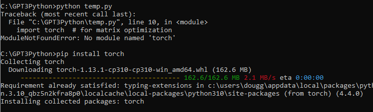
저는 torch 모듈이 없다고 나와서 인스톨 했습니다. pip install torch

이제 import 되는 모듈들을 다 살펴 봤습니다.

 

1. Inputs

여기서는 입력 데이터들에 대한 부분 입니다.

진행하기에 앞서 관련 csv 파일을 구해야 합니다.

 

https://nlp.stanford.edu/projects/snli/

The Stanford Natural Language Processing Group

 

이곳으로 가서 SNLI 1.0 zip 파일을 다운 받으라고 되어 있더라구요.

이 파일을 받고 압축을 풀었더니 3개의 JSON 파일이 있었습니다.

저는 그냥 이중 하나를 CSV 형식으로 convert 했습니다.

 

# input parameters
embedding_cache_path = "data/snli_embedding_cache.pkl"  # embeddings will be saved/loaded here
default_embedding_engine = "babbage-similarity"  # choice of: ada, babbage, curie, davinci
num_pairs_to_embed = 1000  # 1000 is arbitrary - I've gotten it to work with as little as ~100
local_dataset_path = "data/snli_1.0_train_2k.csv"  # download from: https://nlp.stanford.edu/projects/snli/


def process_input_data(df: pd.DataFrame) -> pd.DataFrame:
    # you can customize this to preprocess your own dataset
    # output should be a dataframe with 3 columns: text_1, text_2, label (1 for similar, -1 for dissimilar)
    df["label"] = df["gold_label"]
    df = df[df["label"].isin(["entailment"])]
    df["label"] = df["label"].apply(lambda x: {"entailment": 1, "contradiction": -1}[x])
    df = df.rename(columns={"sentence1": "text_1", "sentence2": "text_2"})
    df = df[["text_1", "text_2", "label"]]
    df = df.head(num_pairs_to_embed)
    return df

여기서 하는 일은 cache 에 있는 데이터를 저장할 pkl 파일을 정하고 사용할 openai 모델을 정했습니다.

그리고 num_pairs_to_embed 변수에 1000을 할당했고 소스 데이터를 local_dataset_path 에 할당했습니다.

 

다음에 process_input_data() 함수가 나오는데요.

pandas 의 DataFrame 형식의 입력값을 받아서 처리한 다음에 다시 DataFrame형식으로 반환합니다.

대개 컬럼 이름들을 바꾸는 거네요.

그리고 DataFrame의 데이터를 1000 (num_pairs_to_embed) 개만 추려서 return 합니다.

 

2. Load and process input data

# load data
df = pd.read_csv(local_dataset_path)

# process input data
df = process_input_data(df)  # this demonstrates training data containing only positives

# view data
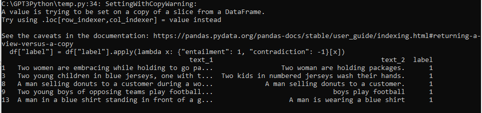
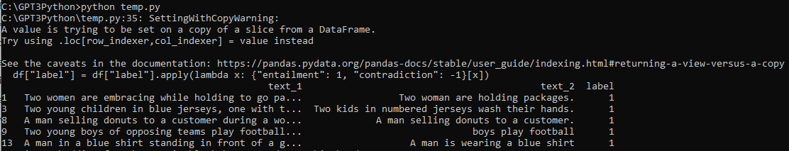
df.head()

이제 파일을 열고 위에 만들었던 함수를 통해 처리한 다음 상위 5개를 출력합니다.

df.head() 는 디폴트로 5개를 출력합니다. head() 안에 숫자를 넣으면 그 숫자만큼 출력합니다.

 

이걸 출력하면 이렇게 됩니다.

3. Split data into training test sets

synethetic negatives나 synethetic positives를 생성하기 전에 데이터를 training과 test sets 들로 구분하는 것은 아주 중요합니다.

 

training data의 text 문자열이 test data에 표시되는 것을 원하지 않을 겁니다. 

contamination이 있는 경우 실제 production 보다 test metrics가 더 좋아 보일 수 있습니다.

 

# split data into train and test sets
test_fraction = 0.5  # 0.5 is fairly arbitrary
random_seed = 123  # random seed is arbitrary, but is helpful in reproducibility
train_df, test_df = train_test_split(
    df, test_size=test_fraction, stratify=df["label"], random_state=random_seed
)
train_df.loc[:, "dataset"] = "train"
test_df.loc[:, "dataset"] = "test"

여기에서는 sklearn.model_selection 모듈의 train_test_split() 함수를 사용해서 데이터를 training test sets로 분리 합니다.

 

4. Generate synthetic negatives

다음은 use case에 맞도록 수정해야 할 필요가 있을 수 있는 코드 입니다.

positives와 negarives 가 있는 데이터를 가지고 있을 경우 건너뛰어도 됩니다.

근데 만약 positives 한 데이터만 가지고 있다면 이 코드를 사용해야 할 것입니다. 

이 코드 블록은 negatives 만 생성할 것입니다.

 

만약 여러분이 multiclass data를 가지고 있다면 여러분은 positives와 negatives 모두를 생성하기를 원할 겁니다.

positives는 레이블들을 공유하는 텍스트로 된 쌍이 될 수 있고 negatives는 레이블을 공유하지 않는 텍스트로 된 쌍이 될 수 있습니다.

 

최종 결과물은 text pair로 된 DataFrame이 될 것입니다. 각 쌍은 -1이나 1이 될 것입니다.

 

# generate negatives
def dataframe_of_negatives(dataframe_of_positives: pd.DataFrame) -> pd.DataFrame:
    """Return dataframe of negative pairs made by combining elements of positive pairs."""
    texts = set(dataframe_of_positives["text_1"].values) | set(
        dataframe_of_positives["text_2"].values
    )
    all_pairs = {(t1, t2) for t1 in texts for t2 in texts if t1 < t2}
    positive_pairs = set(
        tuple(text_pair)
        for text_pair in dataframe_of_positives[["text_1", "text_2"]].values
    )
    negative_pairs = all_pairs - positive_pairs
    df_of_negatives = pd.DataFrame(list(negative_pairs), columns=["text_1", "text_2"])
    df_of_negatives["label"] = -1
    return df_of_negatives

negatives_per_positive = (
    1  # it will work at higher values too, but more data will be slower
)
# generate negatives for training dataset
train_df_negatives = dataframe_of_negatives(train_df)
train_df_negatives["dataset"] = "train"
# generate negatives for test dataset
test_df_negatives = dataframe_of_negatives(test_df)
test_df_negatives["dataset"] = "test"
# sample negatives and combine with positives
train_df = pd.concat(
    [
        train_df,
        train_df_negatives.sample(
            n=len(train_df) * negatives_per_positive, random_state=random_seed
        ),
    ]
)
test_df = pd.concat(
    [
        test_df,
        test_df_negatives.sample(
            n=len(test_df) * negatives_per_positive, random_state=random_seed
        ),
    ]
)

df = pd.concat([train_df, test_df])

 

5. Calculate embeddings and cosine similarities

아래 코드 블럭에서는 임베딩을 저장하기 위한 캐시를 생성합니다. 

이렇게 저장함으로서 다시 임베딩을 얻기 위해 openai api를 호출하면서 비용을 지불하지 않아도 됩니다.

 

# establish a cache of embeddings to avoid recomputing
# cache is a dict of tuples (text, engine) -> embedding
try:
    with open(embedding_cache_path, "rb") as f:
        embedding_cache = pickle.load(f)
except FileNotFoundError:
    precomputed_embedding_cache_path = "https://cdn.openai.com/API/examples/data/snli_embedding_cache.pkl"
    embedding_cache = pd.read_pickle(precomputed_embedding_cache_path)


# this function will get embeddings from the cache and save them there afterward
def get_embedding_with_cache(
    text: str,
    engine: str = default_embedding_engine,
    embedding_cache: dict = embedding_cache,
    embedding_cache_path: str = embedding_cache_path,
) -> list:
    print(f"Getting embedding for {text}")
    if (text, engine) not in embedding_cache.keys():
        # if not in cache, call API to get embedding
        embedding_cache[(text, engine)] = get_embedding(text, engine)
        # save embeddings cache to disk after each update
        with open(embedding_cache_path, "wb") as embedding_cache_file:
            pickle.dump(embedding_cache, embedding_cache_file)
    return embedding_cache[(text, engine)]


# create column of embeddings
for column in ["text_1", "text_2"]:
    df[f"{column}_embedding"] = df[column].apply(get_embedding_with_cache)

# create column of cosine similarity between embeddings
df["cosine_similarity"] = df.apply(
    lambda row: cosine_similarity(row["text_1_embedding"], row["text_2_embedding"]),
    axis=1,
)

 

6. Plot distribution of cosine similarity

이 예제에서는 cosine similarity를 사용하여 텍스트의 유사성을 측정합니다. openai 측의 경험상 대부분의 distance functions (L1, L2, cosine similarity)들은 모두 동일하게 작동한다고 합니다. 임베딩 값은 length 가 1로 정규화 되어 있기 때문에 임베딩에서 cosine similarity는 python의 numpy.dot() 과 동일한 결과를 내 놓습니다.

 

그래프들은 유사한 쌍과 유사하지 않은 쌍에 대한 cosine similarity 분포 사이에 겹치는 정도를 보여 줍니다. 겹치는 부분이 많다면 다른 유사한 쌍보다 cosine similarity가 크고 유사하지 않은 쌍이 많다는 의미 입니다.

 

계산의 정확도는 cosine similarity의 특정 임계치인 X 보다 크면 similar (1)을 예측하고 그렇치 않으면 dissimilar (0)을 예측합니다.

 

# calculate accuracy (and its standard error) of predicting label=1 if similarity>x
# x is optimized by sweeping from -1 to 1 in steps of 0.01
def accuracy_and_se(cosine_similarity: float, labeled_similarity: int) -> Tuple[float]:
    accuracies = []
    for threshold_thousandths in range(-1000, 1000, 1):
        threshold = threshold_thousandths / 1000
        total = 0
        correct = 0
        for cs, ls in zip(cosine_similarity, labeled_similarity):
            total += 1
            if cs > threshold:
                prediction = 1
            else:
                prediction = -1
            if prediction == ls:
                correct += 1
        accuracy = correct / total
        accuracies.append(accuracy)
    a = max(accuracies)
    n = len(cosine_similarity)
    standard_error = (a * (1 - a) / n) ** 0.5  # standard error of binomial
    return a, standard_error


# check that training and test sets are balanced
px.histogram(
    df,
    x="cosine_similarity",
    color="label",
    barmode="overlay",
    width=500,
    facet_row="dataset",
).show()

for dataset in ["train", "test"]:
    data = df[df["dataset"] == dataset]
    a, se = accuracy_and_se(data["cosine_similarity"], data["label"])
    print(f"{dataset} accuracy: {a:0.1%} ± {1.96 * se:0.1%}")

 

여기까지 작성한 코드를 실행 해 봤습니다.

 

처음엔 아래 내용을 출력하더니......

그 다음은 아래와 같은 형식으로 한도 끝도 없이 출력 하더라구요.

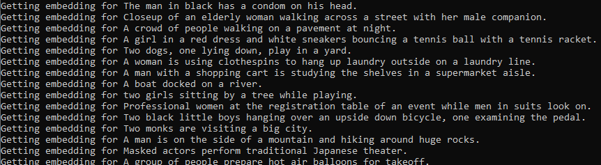
문서에 총 1만줄이 있던데 한줄 한줄 다 처리하느라 시간이 굉장히 많이 걸릴 것 같습니다.

전 3179 줄까지 출력한 후 시간이 너무 걸려서 강제로 중단 했습니다.

 

저는 text-embedding-ada-002 모델을 사용했습니다.

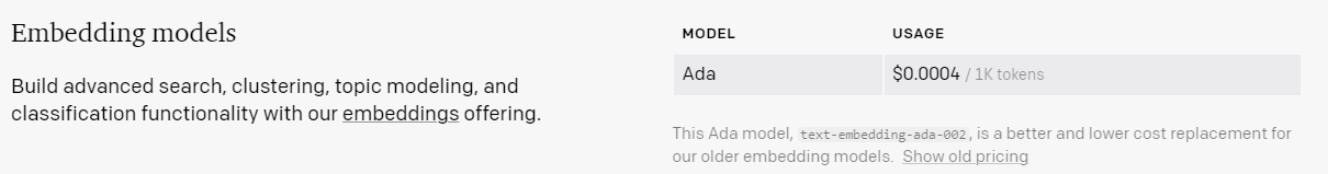
1천개의 토큰당 0.0004불이 과금 되는데 여기까지 저는 0.01불 즉 1센트가 과금 됐습니다.

 

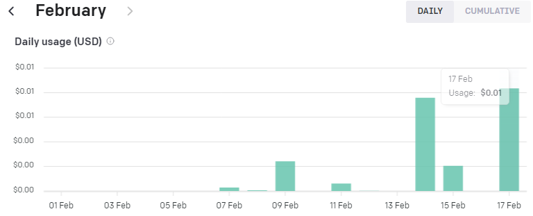
그러면 0.01 / 0.0004 를 하니까 2만 5천 토큰 정도 사용 했나 보네요.

1만줄을 전부 다 하면 한 5센트 이내로 부과 되겠네요.

하여간 시간도 많이 걸리고 과금도 비교적 많이 되니 실행은 마지막에 딱 한번만 해 보기로 하겠습니다.

 

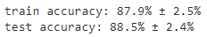
예제 상에는 6 Plot distribution of cosine similarity 에 있는 코드를 실행하면 아래와 같이 나온다고 합니다.

 

 

7. Optimize the matrix using the training data provided

def embedding_multiplied_by_matrix(
    embedding: List[float], matrix: torch.tensor
) -> np.array:
    embedding_tensor = torch.tensor(embedding).float()
    modified_embedding = embedding_tensor @ matrix
    modified_embedding = modified_embedding.detach().numpy()
    return modified_embedding


# compute custom embeddings and new cosine similarities
def apply_matrix_to_embeddings_dataframe(matrix: torch.tensor, df: pd.DataFrame):
    for column in ["text_1_embedding", "text_2_embedding"]:
        df[f"{column}_custom"] = df[column].apply(
            lambda x: embedding_multiplied_by_matrix(x, matrix)
        )
    df["cosine_similarity_custom"] = df.apply(
        lambda row: cosine_similarity(
            row["text_1_embedding_custom"], row["text_2_embedding_custom"]
        ),
        axis=1,
    )

 

def optimize_matrix(
    modified_embedding_length: int = 2048,  # in my brief experimentation, bigger was better (2048 is length of babbage encoding)
    batch_size: int = 100,
    max_epochs: int = 100,
    learning_rate: float = 100.0,  # seemed to work best when similar to batch size - feel free to try a range of values
    dropout_fraction: float = 0.0,  # in my testing, dropout helped by a couple percentage points (definitely not necessary)
    df: pd.DataFrame = df,
    print_progress: bool = True,
    save_results: bool = True,
) -> torch.tensor:
    """Return matrix optimized to minimize loss on training data."""
    run_id = random.randint(0, 2 ** 31 - 1)  # (range is arbitrary)
    # convert from dataframe to torch tensors
    # e is for embedding, s for similarity label
    def tensors_from_dataframe(
        df: pd.DataFrame,
        embedding_column_1: str,
        embedding_column_2: str,
        similarity_label_column: str,
    ) -> Tuple[torch.tensor]:
        e1 = np.stack(np.array(df[embedding_column_1].values))
        e2 = np.stack(np.array(df[embedding_column_2].values))
        s = np.stack(np.array(df[similarity_label_column].astype("float").values))

        e1 = torch.from_numpy(e1).float()
        e2 = torch.from_numpy(e2).float()
        s = torch.from_numpy(s).float()

        return e1, e2, s

    e1_train, e2_train, s_train = tensors_from_dataframe(
        df[df["dataset"] == "train"], "text_1_embedding", "text_2_embedding", "label"
    )
    e1_test, e2_test, s_test = tensors_from_dataframe(
        df[df["dataset"] == "train"], "text_1_embedding", "text_2_embedding", "label"
    )

    # create dataset and loader
    dataset = torch.utils.data.TensorDataset(e1_train, e2_train, s_train)
    train_loader = torch.utils.data.DataLoader(
        dataset, batch_size=batch_size, shuffle=True
    )

    # define model (similarity of projected embeddings)
    def model(embedding_1, embedding_2, matrix, dropout_fraction=dropout_fraction):
        e1 = torch.nn.functional.dropout(embedding_1, p=dropout_fraction)
        e2 = torch.nn.functional.dropout(embedding_2, p=dropout_fraction)
        modified_embedding_1 = e1 @ matrix  # @ is matrix multiplication
        modified_embedding_2 = e2 @ matrix
        similarity = torch.nn.functional.cosine_similarity(
            modified_embedding_1, modified_embedding_2
        )
        return similarity

    # define loss function to minimize
    def mse_loss(predictions, targets):
        difference = predictions - targets
        return torch.sum(difference * difference) / difference.numel()

    # initialize projection matrix
    embedding_length = len(df["text_1_embedding"].values[0])
    matrix = torch.randn(
        embedding_length, modified_embedding_length, requires_grad=True
    )

    epochs, types, losses, accuracies, matrices = [], [], [], [], []
    for epoch in range(1, 1 + max_epochs):
        # iterate through training dataloader
        for a, b, actual_similarity in train_loader:
            # generate prediction
            predicted_similarity = model(a, b, matrix)
            # get loss and perform backpropagation
            loss = mse_loss(predicted_similarity, actual_similarity)
            loss.backward()
            # update the weights
            with torch.no_grad():
                matrix -= matrix.grad * learning_rate
                # set gradients to zero
                matrix.grad.zero_()
        # calculate test loss
        test_predictions = model(e1_test, e2_test, matrix)
        test_loss = mse_loss(test_predictions, s_test)

        # compute custom embeddings and new cosine similarities
        apply_matrix_to_embeddings_dataframe(matrix, df)

        # calculate test accuracy
        for dataset in ["train", "test"]:
            data = df[df["dataset"] == dataset]
            a, se = accuracy_and_se(data["cosine_similarity_custom"], data["label"])

            # record results of each epoch
            epochs.append(epoch)
            types.append(dataset)
            losses.append(loss.item() if dataset == "train" else test_loss.item())
            accuracies.append(a)
            matrices.append(matrix.detach().numpy())

            # optionally print accuracies
            if print_progress is True:
                print(
                    f"Epoch {epoch}/{max_epochs}: {dataset} accuracy: {a:0.1%} ± {1.96 * se:0.1%}"
                )

    data = pd.DataFrame(
        {"epoch": epochs, "type": types, "loss": losses, "accuracy": accuracies}
    )
    data["run_id"] = run_id
    data["modified_embedding_length"] = modified_embedding_length
    data["batch_size"] = batch_size
    data["max_epochs"] = max_epochs
    data["learning_rate"] = learning_rate
    data["dropout_fraction"] = dropout_fraction
    data[
        "matrix"
    ] = matrices  # saving every single matrix can get big; feel free to delete/change
    if save_results is True:
        data.to_csv(f"{run_id}_optimization_results.csv", index=False)

    return data

# example hyperparameter search
# I recommend starting with max_epochs=10 while initially exploring
results = []
max_epochs = 30
dropout_fraction = 0.2
for batch_size, learning_rate in [(10, 10), (100, 100), (1000, 1000)]:
    result = optimize_matrix(
        batch_size=batch_size,
        learning_rate=learning_rate,
        max_epochs=max_epochs,
        dropout_fraction=dropout_fraction,
        save_results=False,
    )
    results.append(result)

runs_df = pd.concat(results)

# plot training loss and test loss over time
px.line(
    runs_df,
    line_group="run_id",
    x="epoch",
    y="loss",
    color="type",
    hover_data=["batch_size", "learning_rate", "dropout_fraction"],
    facet_row="learning_rate",
    facet_col="batch_size",
    width=500,
).show()

# plot accuracy over time
px.line(
    runs_df,
    line_group="run_id",
    x="epoch",
    y="accuracy",
    color="type",
    hover_data=["batch_size", "learning_rate", "dropout_fraction"],
    facet_row="learning_rate",
    facet_col="batch_size",
    width=500,
).show()

 

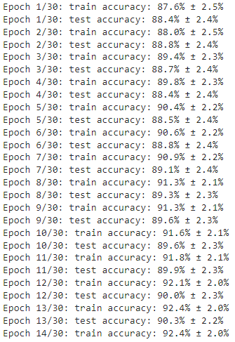
이 부분은 7. Optimize the matrix using the training data provided 부분의 소스코드들 입니다.

 

embedding_multiplied_by_matrix() 함수는 임베딩 값과 matrix 값을 받아서 처리한 다음에 np.array 형식의 결과값을 반환합니다.

 

그 다음 함수는 apply_matrix_to_embeddings_dataframe() 함수로 기존의 임베딩 값과 새로운 cosine similarities 값으로 계산을 하는 일을 합니다.  여기에서 위의 함수인 embedding_multiplied_by_matrix() 함수를 호출한 후 그 결과 값을 받아서 처리합니다.

 

그 다음에도 여러 함수들이 있는데 따로 설명을 하면 너무 길어질 것 같네요.

각자 보면서 분석을 해야 할 것 같습니다.

 

여기까지 실행하면 아래와 같은 결과값을 볼 수 있습니다.

 

8. Plot the before & after, showing the results of the best matrix found during training

matrix 가 좋을 수록 similar pairs 와 dissimilar pairs를 더 명확하게 구분 할 수 있습니다.

 

# apply result of best run to original data
best_run = runs_df.sort_values(by="accuracy", ascending=False).iloc[0]
best_matrix = best_run["matrix"]
apply_matrix_to_embeddings_dataframe(best_matrix, df)

runs_df 는 위에서 정의한 df 변수 이름이고 그 다음의 sort_values() 는 pandas의 함수입니다.

https://pandas.pydata.org/docs/reference/api/pandas.DataFrame.sort_values.html

pandas.DataFrame.sort_values — pandas 1.5.3 documentation

데이터를 sorting 하는 일을 합니다.

이렇게 정렬된 matrix 데이터를 best_matrix에 넣습니다.

그리고 이 정렬된 matrix 값을 7번에서 만든 apply_matrix_to_embeddings_dataframe() 에서 처리하도록 합니다.

 

# plot similarity distribution BEFORE customization
px.histogram(
    df,
    x="cosine_similarity",
    color="label",
    barmode="overlay",
    width=500,
    facet_row="dataset",
).show()

test_df = df[df["dataset"] == "test"]
a, se = accuracy_and_se(test_df["cosine_similarity"], test_df["label"])
print(f"Test accuracy: {a:0.1%} ± {1.96 * se:0.1%}")

# plot similarity distribution AFTER customization
px.histogram(
    df,
    x="cosine_similarity_custom",
    color="label",
    barmode="overlay",
    width=500,
    facet_row="dataset",
).show()

a, se = accuracy_and_se(test_df["cosine_similarity_custom"], test_df["label"])
print(f"Test accuracy after customization: {a:0.1%} ± {1.96 * se:0.1%}")

 

여기서 이용한 함수는 6번에서 만든 accuracy_and_se() 함수 입니다. 정확도를 계산하는 함수였습니다.

 

여기서는 customization이 되기 전의 데이터인 cosine_similarity와 customization이 된 이후의 데이터인 cosine_similarrity_custom에 대해 accuracy_and_se() 함수로 정확도를 계산 한 값을 비교할 수 있도록 해 줍니다.

 

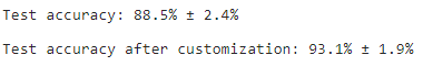
보시는 바와 같이 커스터마이징을 한 데이터가 정확도가 훨씬 높습니다.

 

best_matrix  # this is what you can multiply your embeddings by

이렇게 해서 얻은 best_matrix 를 가지고 사용하면 훨씬 더 좋은 결과를 얻을 수 있습니다.

 

여기까지가 Customizing embeddings 에 대한 내용이었습니다.

 

아주 복잡한 내용 이었던 것 같습니다.

 

몇번 실행해 보면서 코드를 분석해야지 어느 정도 소화를 할 수 있을 것 같습니다.

 

참고로 저는 기존에 1만줄이 있던 소스 파일을 2천줄로 줄여서 사용했습니다.

혹시 도움이 되실까 해서 2천줄로 줄인 csv 파일을 업로드 합니다.

 

snli_1.0_train_2k.csv

1.46MB

그리고 아래는 이 단원을 공부하면서 작성한 소스 코드 전체 입니다.

 

# imports
from typing import List, Tuple  # for type hints

import openai
import numpy as np  # for manipulating arrays
import pandas as pd  # for manipulating data in dataframes
import pickle  # for saving the embeddings cache
import plotly.express as px  # for plots
import random  # for generating run IDs
from sklearn.model_selection import train_test_split  # for splitting train & test data
import torch  # for matrix optimization

from openai.embeddings_utils import get_embedding, cosine_similarity  # for embeddings

def open_file(filepath):
    with open(filepath, 'r', encoding='utf-8') as infile:
        return infile.read()

openai.api_key = open_file('openaiapikey.txt')

# input parameters
embedding_cache_path = "data/snli_embedding_cache.pkl"  # embeddings will be saved/loaded here
#default_embedding_engine = "babbage-similarity"  # choice of: ada, babbage, curie, davinci
#default_embedding_engine = "ada-similarity"
default_embedding_engine = "text-embedding-ada-002"
num_pairs_to_embed = 1000  # 1000 is arbitrary - I've gotten it to work with as little as ~100
local_dataset_path = "data/snli_1.0_train_2k.csv"  # download from: https://nlp.stanford.edu/projects/snli/


def process_input_data(df: pd.DataFrame) -> pd.DataFrame:
    # you can customize this to preprocess your own dataset
    # output should be a dataframe with 3 columns: text_1, text_2, label (1 for similar, -1 for dissimilar)
    df["label"] = df["gold_label"]
    df = df[df["label"].isin(["entailment"])]
    df["label"] = df["label"].apply(lambda x: {"entailment": 1, "contradiction": -1}[x])
    df = df.rename(columns={"sentence1": "text_1", "sentence2": "text_2"})
    df = df[["text_1", "text_2", "label"]]
    df = df.head(num_pairs_to_embed)
    return df
    
# load data
df = pd.read_csv(local_dataset_path)

# process input data
df = process_input_data(df)  # this demonstrates training data containing only positives

# view data
result = df.head()

print(result)

# split data into train and test sets
test_fraction = 0.5  # 0.5 is fairly arbitrary
random_seed = 123  # random seed is arbitrary, but is helpful in reproducibility
train_df, test_df = train_test_split(
    df, test_size=test_fraction, stratify=df["label"], random_state=random_seed
)
train_df.loc[:, "dataset"] = "train"
test_df.loc[:, "dataset"] = "test"

# generate negatives
def dataframe_of_negatives(dataframe_of_positives: pd.DataFrame) -> pd.DataFrame:
    """Return dataframe of negative pairs made by combining elements of positive pairs."""
    texts = set(dataframe_of_positives["text_1"].values) | set(
        dataframe_of_positives["text_2"].values
    )
    all_pairs = {(t1, t2) for t1 in texts for t2 in texts if t1 < t2}
    positive_pairs = set(
        tuple(text_pair)
        for text_pair in dataframe_of_positives[["text_1", "text_2"]].values
    )
    negative_pairs = all_pairs - positive_pairs
    df_of_negatives = pd.DataFrame(list(negative_pairs), columns=["text_1", "text_2"])
    df_of_negatives["label"] = -1
    return df_of_negatives
    
negatives_per_positive = (
    1  # it will work at higher values too, but more data will be slower
)
# generate negatives for training dataset
train_df_negatives = dataframe_of_negatives(train_df)
train_df_negatives["dataset"] = "train"
# generate negatives for test dataset
test_df_negatives = dataframe_of_negatives(test_df)
test_df_negatives["dataset"] = "test"
# sample negatives and combine with positives
train_df = pd.concat(
    [
        train_df,
        train_df_negatives.sample(
            n=len(train_df) * negatives_per_positive, random_state=random_seed
        ),
    ]
)
test_df = pd.concat(
    [
        test_df,
        test_df_negatives.sample(
            n=len(test_df) * negatives_per_positive, random_state=random_seed
        ),
    ]
)

df = pd.concat([train_df, test_df])

# establish a cache of embeddings to avoid recomputing
# cache is a dict of tuples (text, engine) -> embedding
try:
    with open(embedding_cache_path, "rb") as f:
        embedding_cache = pickle.load(f)
except FileNotFoundError:
    precomputed_embedding_cache_path = "https://cdn.openai.com/API/examples/data/snli_embedding_cache.pkl"
    embedding_cache = pd.read_pickle(precomputed_embedding_cache_path)


# this function will get embeddings from the cache and save them there afterward
def get_embedding_with_cache(
    text: str,
    engine: str = default_embedding_engine,
    embedding_cache: dict = embedding_cache,
    embedding_cache_path: str = embedding_cache_path,
) -> list:
    print(f"Getting embedding for {text}")
    if (text, engine) not in embedding_cache.keys():
        # if not in cache, call API to get embedding
        embedding_cache[(text, engine)] = get_embedding(text, engine)
        # save embeddings cache to disk after each update
        with open(embedding_cache_path, "wb") as embedding_cache_file:
            pickle.dump(embedding_cache, embedding_cache_file)
    return embedding_cache[(text, engine)]


# create column of embeddings
for column in ["text_1", "text_2"]:
    df[f"{column}_embedding"] = df[column].apply(get_embedding_with_cache)

# create column of cosine similarity between embeddings
df["cosine_similarity"] = df.apply(
    lambda row: cosine_similarity(row["text_1_embedding"], row["text_2_embedding"]),
    axis=1,
)

# calculate accuracy (and its standard error) of predicting label=1 if similarity>x
# x is optimized by sweeping from -1 to 1 in steps of 0.01
def accuracy_and_se(cosine_similarity: float, labeled_similarity: int) -> Tuple[float]:
    accuracies = []
    for threshold_thousandths in range(-1000, 1000, 1):
        threshold = threshold_thousandths / 1000
        total = 0
        correct = 0
        for cs, ls in zip(cosine_similarity, labeled_similarity):
            total += 1
            if cs > threshold:
                prediction = 1
            else:
                prediction = -1
            if prediction == ls:
                correct += 1
        accuracy = correct / total
        accuracies.append(accuracy)
    a = max(accuracies)
    n = len(cosine_similarity)
    standard_error = (a * (1 - a) / n) ** 0.5  # standard error of binomial
    return a, standard_error


# check that training and test sets are balanced
px.histogram(
    df,
    x="cosine_similarity",
    color="label",
    barmode="overlay",
    width=500,
    facet_row="dataset",
).show()

for dataset in ["train", "test"]:
    data = df[df["dataset"] == dataset]
    a, se = accuracy_and_se(data["cosine_similarity"], data["label"])
    print(f"{dataset} accuracy: {a:0.1%} ± {1.96 * se:0.1%}")

def embedding_multiplied_by_matrix(
    embedding: List[float], matrix: torch.tensor
) -> np.array:
    embedding_tensor = torch.tensor(embedding).float()
    modified_embedding = embedding_tensor @ matrix
    modified_embedding = modified_embedding.detach().numpy()
    return modified_embedding


# compute custom embeddings and new cosine similarities
def apply_matrix_to_embeddings_dataframe(matrix: torch.tensor, df: pd.DataFrame):
    for column in ["text_1_embedding", "text_2_embedding"]:
        df[f"{column}_custom"] = df[column].apply(
            lambda x: embedding_multiplied_by_matrix(x, matrix)
        )
    df["cosine_similarity_custom"] = df.apply(
        lambda row: cosine_similarity(
            row["text_1_embedding_custom"], row["text_2_embedding_custom"]
        ),
        axis=1,
    )
    
def optimize_matrix(
    modified_embedding_length: int = 2048,  # in my brief experimentation, bigger was better (2048 is length of babbage encoding)
    batch_size: int = 100,
    max_epochs: int = 100,
    learning_rate: float = 100.0,  # seemed to work best when similar to batch size - feel free to try a range of values
    dropout_fraction: float = 0.0,  # in my testing, dropout helped by a couple percentage points (definitely not necessary)
    df: pd.DataFrame = df,
    print_progress: bool = True,
    save_results: bool = True,
) -> torch.tensor:
    """Return matrix optimized to minimize loss on training data."""
    run_id = random.randint(0, 2 ** 31 - 1)  # (range is arbitrary)
    # convert from dataframe to torch tensors
    # e is for embedding, s for similarity label
    def tensors_from_dataframe(
        df: pd.DataFrame,
        embedding_column_1: str,
        embedding_column_2: str,
        similarity_label_column: str,
    ) -> Tuple[torch.tensor]:
        e1 = np.stack(np.array(df[embedding_column_1].values))
        e2 = np.stack(np.array(df[embedding_column_2].values))
        s = np.stack(np.array(df[similarity_label_column].astype("float").values))

        e1 = torch.from_numpy(e1).float()
        e2 = torch.from_numpy(e2).float()
        s = torch.from_numpy(s).float()

        return e1, e2, s

    e1_train, e2_train, s_train = tensors_from_dataframe(
        df[df["dataset"] == "train"], "text_1_embedding", "text_2_embedding", "label"
    )
    e1_test, e2_test, s_test = tensors_from_dataframe(
        df[df["dataset"] == "train"], "text_1_embedding", "text_2_embedding", "label"
    )

    # create dataset and loader
    dataset = torch.utils.data.TensorDataset(e1_train, e2_train, s_train)
    train_loader = torch.utils.data.DataLoader(
        dataset, batch_size=batch_size, shuffle=True
    )

    # define model (similarity of projected embeddings)
    def model(embedding_1, embedding_2, matrix, dropout_fraction=dropout_fraction):
        e1 = torch.nn.functional.dropout(embedding_1, p=dropout_fraction)
        e2 = torch.nn.functional.dropout(embedding_2, p=dropout_fraction)
        modified_embedding_1 = e1 @ matrix  # @ is matrix multiplication
        modified_embedding_2 = e2 @ matrix
        similarity = torch.nn.functional.cosine_similarity(
            modified_embedding_1, modified_embedding_2
        )
        return similarity

    # define loss function to minimize
    def mse_loss(predictions, targets):
        difference = predictions - targets
        return torch.sum(difference * difference) / difference.numel()

    # initialize projection matrix
    embedding_length = len(df["text_1_embedding"].values[0])
    matrix = torch.randn(
        embedding_length, modified_embedding_length, requires_grad=True
    )

    epochs, types, losses, accuracies, matrices = [], [], [], [], []
    for epoch in range(1, 1 + max_epochs):
        # iterate through training dataloader
        for a, b, actual_similarity in train_loader:
            # generate prediction
            predicted_similarity = model(a, b, matrix)
            # get loss and perform backpropagation
            loss = mse_loss(predicted_similarity, actual_similarity)
            loss.backward()
            # update the weights
            with torch.no_grad():
                matrix -= matrix.grad * learning_rate
                # set gradients to zero
                matrix.grad.zero_()
        # calculate test loss
        test_predictions = model(e1_test, e2_test, matrix)
        test_loss = mse_loss(test_predictions, s_test)

        # compute custom embeddings and new cosine similarities
        apply_matrix_to_embeddings_dataframe(matrix, df)

        # calculate test accuracy
        for dataset in ["train", "test"]:
            data = df[df["dataset"] == dataset]
            a, se = accuracy_and_se(data["cosine_similarity_custom"], data["label"])

            # record results of each epoch
            epochs.append(epoch)
            types.append(dataset)
            losses.append(loss.item() if dataset == "train" else test_loss.item())
            accuracies.append(a)
            matrices.append(matrix.detach().numpy())

            # optionally print accuracies
            if print_progress is True:
                print(
                    f"Epoch {epoch}/{max_epochs}: {dataset} accuracy: {a:0.1%} ± {1.96 * se:0.1%}"
                )

    data = pd.DataFrame(
        {"epoch": epochs, "type": types, "loss": losses, "accuracy": accuracies}
    )
    data["run_id"] = run_id
    data["modified_embedding_length"] = modified_embedding_length
    data["batch_size"] = batch_size
    data["max_epochs"] = max_epochs
    data["learning_rate"] = learning_rate
    data["dropout_fraction"] = dropout_fraction
    data[
        "matrix"
    ] = matrices  # saving every single matrix can get big; feel free to delete/change
    if save_results is True:
        data.to_csv(f"{run_id}_optimization_results.csv", index=False)

    return data
    
# example hyperparameter search
# I recommend starting with max_epochs=10 while initially exploring
results = []
max_epochs = 30
dropout_fraction = 0.2
for batch_size, learning_rate in [(10, 10), (100, 100), (1000, 1000)]:
    result = optimize_matrix(
        batch_size=batch_size,
        learning_rate=learning_rate,
        max_epochs=max_epochs,
        dropout_fraction=dropout_fraction,
        save_results=False,
    )
    results.append(result)
    
runs_df = pd.concat(results)

# plot training loss and test loss over time
px.line(
    runs_df,
    line_group="run_id",
    x="epoch",
    y="loss",
    color="type",
    hover_data=["batch_size", "learning_rate", "dropout_fraction"],
    facet_row="learning_rate",
    facet_col="batch_size",
    width=500,
).show()

# plot accuracy over time
px.line(
    runs_df,
    line_group="run_id",
    x="epoch",
    y="accuracy",
    color="type",
    hover_data=["batch_size", "learning_rate", "dropout_fraction"],
    facet_row="learning_rate",
    facet_col="batch_size",
    width=500,
).show()

# apply result of best run to original data
best_run = runs_df.sort_values(by="accuracy", ascending=False).iloc[0]
best_matrix = best_run["matrix"]
apply_matrix_to_embeddings_dataframe(best_matrix, df)

# plot similarity distribution BEFORE customization
px.histogram(
    df,
    x="cosine_similarity",
    color="label",
    barmode="overlay",
    width=500,
    facet_row="dataset",
).show()

test_df = df[df["dataset"] == "test"]
a, se = accuracy_and_se(test_df["cosine_similarity"], test_df["label"])
print(f"Test accuracy: {a:0.1%} ± {1.96 * se:0.1%}")

# plot similarity distribution AFTER customization
px.histogram(
    df,
    x="cosine_similarity_custom",
    color="label",
    barmode="overlay",
    width=500,
    facet_row="dataset",
).show()

a, se = accuracy_and_se(test_df["cosine_similarity_custom"], test_df["label"])
print(f"Test accuracy after customization: {a:0.1%} ± {1.96 * se:0.1%}")

best_matrix  # this is what you can multiply your embeddings by