

16.4. Natural Language Inference and the Dataset — Dive into Deep Learning 1.0.3 documentation
d2l.ai
16.5. Natural Language Inference: Using Attention
We introduced the natural language inference task and the SNLI dataset in Section 16.4. In view of many models that are based on complex and deep architectures, Parikh et al. (2016) proposed to address natural language inference with attention mechanisms and called it a “decomposable attention model”. This results in a model without recurrent or convolutional layers, achieving the best result at the time on the SNLI dataset with much fewer parameters. In this section, we will describe and implement this attention-based method (with MLPs) for natural language inference, as depicted in Fig. 16.5.1.
섹션 16.4에서 자연어 추론 작업과 SNLI 데이터 세트를 소개했습니다. 복잡하고 심층적인 아키텍처를 기반으로 하는 많은 모델을 고려하여 Parikh et al. (2016)은 Attention 메커니즘을 통해 자연어 추론을 처리할 것을 제안하고 이를 "분해 가능한 Attention 모델"이라고 불렀습니다. 그 결과 순환 또는 컨벌루션 레이어가 없는 모델이 생성되어 훨씬 적은 매개변수를 사용하여 SNLI 데이터세트에서 당시 최상의 결과를 얻을 수 있습니다. 이 섹션에서는 그림 16.5.1에 설명된 대로 자연어 추론을 위한 Attention 기반 방법(MLP 사용)을 설명하고 구현합니다.

16.5.1. The Model
Simpler than preserving the order of tokens in premises and hypotheses, we can just align tokens in one text sequence to every token in the other, and vice versa, then compare and aggregate such information to predict the logical relationships between premises and hypotheses. Similar to alignment of tokens between source and target sentences in machine translation, the alignment of tokens between premises and hypotheses can be neatly accomplished by attention mechanisms.
전제와 가설에서 토큰의 순서를 유지하는 것보다 더 간단한 것은 한 텍스트 시퀀스의 토큰을 다른 텍스트 시퀀스의 모든 토큰에 정렬하고 그 반대의 경우도 마찬가지입니다. 그런 다음 이러한 정보를 비교하고 집계하여 전제와 가설 사이의 논리적 관계를 예측할 수 있습니다. 기계 번역에서 소스 문장과 대상 문장 사이의 토큰 정렬과 유사하게 전제와 가설 사이의 토큰 정렬은 어텐션 메커니즘을 통해 깔끔하게 수행될 수 있습니다.

Fig. 16.5.2 depicts the natural language inference method using attention mechanisms. At a high level, it consists of three jointly trained steps: attending, comparing, and aggregating. We will illustrate them step by step in the following.
그림 16.5.2는 Attention 메커니즘을 이용한 자연어 추론 방법을 보여줍니다. high level concept을 보면 참석 attending, 비교 comparing, 집계 aggregating라는 세 가지 공동 훈련 단계로 구성됩니다. 다음에서는 이를 단계별로 설명하겠습니다.
import torch
from torch import nn
from torch.nn import functional as F
from d2l import torch as d2l
16.5.1.1. Attending
The first step is to align tokens in one text sequence to each token in the other sequence. Suppose that the premise is “i do need sleep” and the hypothesis is “i am tired”. Due to semantical similarity, we may wish to align “i” in the hypothesis with “i” in the premise, and align “tired” in the hypothesis with “sleep” in the premise. Likewise, we may wish to align “i” in the premise with “i” in the hypothesis, and align “need” and “sleep” in the premise with “tired” in the hypothesis. Note that such alignment is soft using weighted average, where ideally large weights are associated with the tokens to be aligned. For ease of demonstration, Fig. 16.5.2 shows such alignment in a hard way.
첫 번째 단계는 한 텍스트 시퀀스의 토큰을 다른 시퀀스의 각 토큰에 정렬하는 것입니다. 전제가 "i do need sleep"이고 가설은 "i am tired"라고 가정해보자. 의미적 유사성으로 인해 가설의 "i"를 전제의 "i"와 정렬하고 가설의 "tired"를 전제의 "sleep"과 정렬할 수 있습니다. 마찬가지로, 전제의 "i"를 가설의 "i"와 정렬하고 전제의 "need"와 "sleep"을 가설의 "tired"와 정렬할 수 있습니다. 이러한 정렬은 가중 평균을 사용하여 유연하게 이루어지며, 이상적으로는 큰 가중치가 정렬할 토큰과 연관되어 있습니다. 설명을 쉽게 하기 위해 그림 16.5.2에서는 이러한 정렬을 어려운 방식으로 보여줍니다.
Now we describe the soft alignment using attention mechanisms in more detail. Denote by A=(a1,...,am) and B=(b1,...,bn) the premise and hypothesis, whose number of tokens are m and n, respectively, where ai,bj∈ℝ**d (i=1,...,m,j=1,...,n) is a d-dimensional word vector. For soft alignment, we compute the attention weights eij∈ℝ as
이제 attention 메커니즘을 사용하여 소프트 정렬을 더 자세히 설명합니다. 전제와 가설을 A=(a1,...,am) 및 B=(b1,...,bn)으로 표시합니다. 여기서 토큰 수는 각각 m과 n입니다. 여기서 ai,bj∈ℝ**d (i=1,...,m,j=1,...,n)은 d차원 단어 벡터입니다. 소프트 정렬을 위해 관심 가중치 attention weights eij∈ℝ를 다음과 같이 계산합니다.

where the function f is an MLP defined in the following mlp function. The output dimension of f is specified by the num_hiddens argument of mlp.
여기서 함수 f는 다음 mlp 함수에 정의된 MLP입니다. f의 출력 차원은 mlp의 num_hiddens 인수로 지정됩니다.
def mlp(num_inputs, num_hiddens, flatten):
    net = []
    net.append(nn.Dropout(0.2))
    net.append(nn.Linear(num_inputs, num_hiddens))
    net.append(nn.ReLU())
    if flatten:
        net.append(nn.Flatten(start_dim=1))
    net.append(nn.Dropout(0.2))
    net.append(nn.Linear(num_hiddens, num_hiddens))
    net.append(nn.ReLU())
    if flatten:
        net.append(nn.Flatten(start_dim=1))
    return nn.Sequential(*net)
이 코드는 다층 퍼셉트론(MLP) 네트워크를 정의하는 함수인 mlp를 생성하는 파이토치 코드입니다. 이 함수는 네트워크의 구조를 정의하고 반환합니다. 코드의 작동 방식을 설명하겠습니다.
- 함수 정의:
- def mlp(num_inputs, num_hiddens, flatten):: MLP 네트워크를 정의하는 함수입니다. 인자로 입력 특성의 수(num_inputs), 은닉층의 유닛 수(num_hiddens), 평탄화 여부(flatten)를 받습니다.
- 네트워크 구성:
- net = []: 빈 리스트를 생성하여 네트워크 레이어를 순서대로 추가할 예정입니다.
- net.append(nn.Dropout(0.2)): 드롭아웃 레이어를 추가합니다. 드롭아웃은 과적합을 방지하기 위해 사용됩니다.
- net.append(nn.Linear(num_inputs, num_hiddens)): 완전 연결 레이어를 추가합니다. 입력 특성 수에서 은닉층 유닛 수로 연결됩니다.
- net.append(nn.ReLU()): ReLU 활성화 함수를 추가합니다. 이 함수는 비선형성을 네트워크에 추가합니다.
- if flatten: ...: 만약 flatten이 True라면, 평탄화 레이어(nn.Flatten)를 추가합니다. 평탄화는 2D 입력을 1D로 변환합니다.
- 위의 네 레이어를 한 번 더 추가합니다. 이것은 두 번째 은닉층과 ReLU 활성화 함수를 의미합니다.
- 네트워크 반환:
- return nn.Sequential(*net): 정의한 레이어들을 nn.Sequential 컨테이너로 묶어서 반환합니다. 이것은 순차적으로 레이어가 실행되는 MLP 네트워크를 나타냅니다.
결과적으로, 이 함수는 주어진 입력 특성 수와 은닉층 유닛 수에 따라 다층 퍼셉트론(MLP) 네트워크를 생성하고, 평탄화 여부에 따라 네트워크 구조를 조절하여 반환합니다.
It should be highlighted that, in (16.5.1) f takes inputs ai and bj separately rather than takes a pair of them together as input. This decomposition trick leads to only m+n applications (linear complexity) of f rather than mn applications (quadratic complexity).
(16.5.1)에서 f는 ai와 bj를 입력으로 함께 사용하는 대신 입력 ai와 bj를 별도로 사용한다는 점을 강조해야 합니다. 이 분해 트릭은 mn 적용(2차 복잡도)이 아닌 f의 m+n 적용(선형 복잡도)만을 초래합니다.
Normalizing the attention weights in (16.5.1), we compute the weighted average of all the token vectors in the hypothesis to obtain representation of the hypothesis that is softly aligned with the token indexed by i in the premise:
(16.5.1)에서 어텐션 가중치를 정규화하여 가설의 모든 토큰 벡터의 가중 평균을 계산하여 전제에서 i로 인덱스된 토큰과 부드럽게 정렬되는 가설의 표현을 얻습니다.

Likewise, we compute soft alignment of premise tokens for each token indexed by j in the hypothesis:
마찬가지로 가설에서 j로 색인된 각 토큰에 대한 전제 토큰의 소프트 정렬을 계산합니다.

Below we define the Attend class to compute the soft alignment of hypotheses (beta) with input premises A and soft alignment of premises (alpha) with input hypotheses B.
아래에서는 입력 전제 A와 가설(베타)의 소프트 정렬 및 입력 가설 B와 전제(알파)의 소프트 정렬을 계산하기 위해 Attend 클래스를 정의합니다.
class Attend(nn.Module):
    def __init__(self, num_inputs, num_hiddens, **kwargs):
        super(Attend, self).__init__(**kwargs)
        self.f = mlp(num_inputs, num_hiddens, flatten=False)

    def forward(self, A, B):
        # Shape of `A`/`B`: (`batch_size`, no. of tokens in sequence A/B,
        # `embed_size`)
        # Shape of `f_A`/`f_B`: (`batch_size`, no. of tokens in sequence A/B,
        # `num_hiddens`)
        f_A = self.f(A)
        f_B = self.f(B)
        # Shape of `e`: (`batch_size`, no. of tokens in sequence A,
        # no. of tokens in sequence B)
        e = torch.bmm(f_A, f_B.permute(0, 2, 1))
        # Shape of `beta`: (`batch_size`, no. of tokens in sequence A,
        # `embed_size`), where sequence B is softly aligned with each token
        # (axis 1 of `beta`) in sequence A
        beta = torch.bmm(F.softmax(e, dim=-1), B)
        # Shape of `alpha`: (`batch_size`, no. of tokens in sequence B,
        # `embed_size`), where sequence A is softly aligned with each token
        # (axis 1 of `alpha`) in sequence B
        alpha = torch.bmm(F.softmax(e.permute(0, 2, 1), dim=-1), A)
        return beta, alpha
이 코드는 "Attend"라는 클래스를 정의하는 파이토치 코드로, 시퀀스 A와 시퀀스 B 간의 어텐션 메커니즘을 구현합니다. 코드의 작동 방식을 설명하겠습니다.
- 클래스 정의:
- class Attend(nn.Module):: Attend 클래스를 정의합니다. 이 클래스는 파이토치의 nn.Module을 상속합니다.
- 생성자(__init__) 메서드:
- def __init__(self, num_inputs, num_hiddens, **kwargs):: Attend 클래스의 생성자 메서드입니다. 인자로 num_inputs (입력 특성의 수), num_hiddens (은닉층의 유닛 수)를 받습니다.
- self.f = mlp(num_inputs, num_hiddens, flatten=False): Attend 클래스 내에서 사용할 MLP 네트워크 f를 생성합니다. mlp 함수를 호출하여 생성한 MLP 네트워크를 self.f로 저장합니다.
- forward 메서드:
- def forward(self, A, B):: Attend 클래스의 forward 메서드입니다. 인자로 시퀀스 A와 시퀀스 B를 받습니다.
- f_A = self.f(A), f_B = self.f(B): 시퀀스 A와 시퀀스 B에 각각 MLP 네트워크를 적용하여 특성을 추출합니다.
- e = torch.bmm(f_A, f_B.permute(0, 2, 1)): 두 시퀀스 간의 유사도 점수를 계산합니다. f_A와 f_B의 내적을 계산하여 어텐션 스코어 행렬 e를 얻습니다.
- beta = torch.bmm(F.softmax(e, dim=-1), B): 시퀀스 A에 대한 부드러운 어텐션 가중치를 계산하고, 이를 기반으로 시퀀스 B를 정렬합니다.
- alpha = torch.bmm(F.softmax(e.permute(0, 2, 1), dim=-1), A): 시퀀스 B에 대한 부드러운 어텐션 가중치를 계산하고, 이를 기반으로 시퀀스 A를 정렬합니다.
- return beta, alpha: 계산된 어텐션 가중치인 beta와 alpha를 반환합니다.
결과적으로, 이 코드는 시퀀스 A와 시퀀스 B 간의 어텐션을 계산하는 Attend 클래스를 정의하고, forward 메서드를 통해 어텐션 가중치를 계산하여 반환합니다. 이것은 주로 자연어 처리 태스크에서 활용되는 어텐션 메커니즘의 일부분입니다.
https://pytorch.org/docs/stable/generated/torch.bmm.html
torch.bmm — PyTorch 2.0 documentation
Shortcuts
pytorch.org
https://blog.naver.com/gksthf4140/222986529109
(DL). torch - 선형 계층 ( matmul, bmm, nn.Module, nn.Linear, nn.Parameters )
[ 행렬 곱 ] 행렬의 곱은 inner product 또는 dot product 라고 불림 배치 행렬 곱 딥러닝을 수행할 때 Ba...
blog.naver.com
https://pytorch.org/docs/stable/generated/torch.permute.html
torch.permute — PyTorch 2.0 documentation
Shortcuts
pytorch.org
http://iambeginnerdeveloper.tistory.com/215
[pytorch] transpose, permute 함수
pytorch로 permute 함수를 사용하다가 transpose랑 비슷한 것 같은데 정확히 차이를 모르고 있구나 싶어서 찾아보고 기록하기 위해 해당 포스트를 작성하게 되었다. ◾ permute() 먼저, permute 함수는 모든
iambeginnerdeveloper.tistory.com
https://pytorch.org/docs/stable/generated/torch.nn.Softmax.html
Softmax — PyTorch 2.0 documentation
Shortcuts
pytorch.org
16.5.1.2. Comparing
In the next step, we compare a token in one sequence with the other sequence that is softly aligned with that token. Note that in soft alignment, all the tokens from one sequence, though with probably different attention weights, will be compared with a token in the other sequence. For easy of demonstration, Fig. 16.5.2 pairs tokens with aligned tokens in a hard way. For example, suppose that the attending step determines that “need” and “sleep” in the premise are both aligned with “tired” in the hypothesis, the pair “tired–need sleep” will be compared.
다음 단계에서는 한 시퀀스의 토큰을 해당 토큰과 소프트하게 정렬된 다른 시퀀스와 비교합니다. 소프트 정렬에서는 주의 가중치가 다를지라도 한 시퀀스의 모든 토큰이 다른 시퀀스의 토큰과 비교됩니다. 시연을 쉽게 하기 위해 그림 16.5.2에서는 토큰과 정렬된 토큰을 hard way으로 쌍으로 연결합니다. 예를 들어, 참석 attending 단계에서 전제 premise 의 "need"와 "sleep"이 모두 가설 hypothesis의 "tired"과 일치한다고 판단한다고 가정하면 "tired–need sleep" 쌍이 비교됩니다.
In the comparing step, we feed the concatenation (operator [⋅,⋅]) of tokens from one sequence and aligned tokens from the other sequence into a function g (an MLP):
비교 단계에서는 한 시퀀스의 토큰과 다른 시퀀스의 정렬된 토큰을 함수 g(MLP)에 연결(연산자 [⋅,⋅])합니다.

Soft Alignment란?
'Soft alignment'은 주어진 두 시퀀스 간의 상관 관계를 나타내는 방법 중 하나입니다. 이것은 자연어 처리와 기계 학습에서 자주 사용되며, 주로 시퀀스-시퀀스 모델, 언어 모델, 번역 모델 등에서 사용됩니다.
'Soft alignment'은 두 시퀀스 사이의 상호작용을 '단단한' 매칭이 아니라 각 요소 사이의 '소프트한' 매칭으로 표현합니다. 이것은 각 요소가 다른 요소와 얼마나 관련이 있는지를 확률적으로 표현합니다. 주로 다음과 같은 상황에서 사용됩니다.
- 번역 모델 (Machine Translation): 소스 언어와 타겟 언어 간의 문장을 번역할 때, 각 소스 단어가 타겟 문장에서 어떻게 매핑되는지를 나타냅니다. Soft alignment은 각 소스 단어가 다른 언어의 단어와 얼마나 연관되어 있는지를 확률적으로 표현하여 번역 모델을 개선하는 데 사용됩니다.
- 질의응답 (Question Answering): 주어진 질문과 문서에서 답변을 찾을 때, 문서의 각 단어가 질문과 어떻게 관련되어 있는지를 나타냅니다. 이것은 문서 내에서 답변을 찾는 데 도움이 됩니다.
- 기계 독해 (Machine Reading Comprehension): 주어진 텍스트에서 특정 질문에 대한 답변을 찾는 작업에서 사용됩니다. 각 문장 또는 문단의 각 단어가 질문과 어떻게 관련되어 있는지를 표현합니다.
Soft alignment을 사용하면 정보를 효과적으로 전달하고 시퀀스 간의 관계를 모델링할 수 있습니다. 이것은 주어진 작업에 따라 적절한 가중치를 각 요소에 할당하는 데 도움이 됩니다. Soft alignment은 주로 확률 분포 또는 어텐션 메커니즘과 같은 방법을 사용하여 구현됩니다. 이러한 메커니즘은 각 요소 간의 상호작용을 확률적으로 모델링하는 방법을 제공하며, 이를 통해 다양한 자연어 처리 작업을 효과적으로 수행할 수 있게 됩니다.
In (16.5.4), vA,i is the comparison between token i in the premise and all the hypothesis tokens that are softly aligned with token i; while vB,j is the comparison between token j in the hypothesis and all the premise tokens that are softly aligned with token j. The following Compare class defines such as comparing step.
(16.5.4)에서 vA,i는 전제의 토큰 i와 토큰 i와 부드럽게 정렬된 모든 가설 토큰 간의 비교입니다. vB,j는 가설의 토큰 j와 토큰 j와 부드럽게 정렬된 모든 전제 토큰 간의 비교입니다. 다음 Compare 클래스는 비교 단계 등을 정의합니다.
class Compare(nn.Module):
    def __init__(self, num_inputs, num_hiddens, **kwargs):
        super(Compare, self).__init__(**kwargs)
        self.g = mlp(num_inputs, num_hiddens, flatten=False)

    def forward(self, A, B, beta, alpha):
        V_A = self.g(torch.cat([A, beta], dim=2))
        V_B = self.g(torch.cat([B, alpha], dim=2))
        return V_A, V_B
이 코드는 "Compare"라는 클래스를 정의하는 파이토치 코드로, 두 시퀀스 A와 B 간의 비교를 수행하는 부분입니다. 코드의 작동 방식을 설명하겠습니다.
- 클래스 정의:
- class Compare(nn.Module):: Compare 클래스를 정의합니다. 이 클래스는 파이토치의 nn.Module을 상속합니다.
- 생성자(__init__) 메서드:
- def __init__(self, num_inputs, num_hiddens, **kwargs):: Compare 클래스의 생성자 메서드입니다. 인자로 num_inputs (입력 특성의 수), num_hiddens (은닉층의 유닛 수)를 받습니다.
- self.g = mlp(num_inputs, num_hiddens, flatten=False): Compare 클래스 내에서 사용할 MLP 네트워크 g를 생성합니다. mlp 함수를 호출하여 생성한 MLP 네트워크를 self.g로 저장합니다.
- forward 메서드:
- def forward(self, A, B, beta, alpha):: Compare 클래스의 forward 메서드입니다. 인자로 시퀀스 A, 시퀀스 B, 그리고 Attend 클래스에서 얻은 어텐션 가중치 beta와 alpha를 받습니다.
- V_A = self.g(torch.cat([A, beta], dim=2)): 시퀀스 A와 해당 시퀀스에 부드러운 어텐션을 적용한 beta를 합치고, MLP 네트워크 g를 사용하여 시퀀스 A에 대한 특성 벡터 V_A를 계산합니다.
- V_B = self.g(torch.cat([B, alpha], dim=2)): 시퀀스 B와 해당 시퀀스에 부드러운 어텐션을 적용한 alpha를 합치고, MLP 네트워크 g를 사용하여 시퀀스 B에 대한 특성 벡터 V_B를 계산합니다.
- return V_A, V_B: 계산된 시퀀스 A와 B의 특성 벡터 V_A와 V_B를 반환합니다.
결과적으로, 이 코드는 두 시퀀스 A와 B 간의 비교를 수행하는 Compare 클래스를 정의하고, forward 메서드를 통해 각 시퀀스에 대한 특성 벡터 V_A와 V_B를 계산하여 반환합니다. 이것은 주로 자연어 처리 태스크에서 활용되는 비교 메커니즘의 일부분입니다.
16.5.1.3. Aggregating
With two sets of comparison vectors vA,i (i=1,…,m) and vB,j (j=1,…,n) on hand, in the last step we will aggregate such information to infer the logical relationship. We begin by summing up both sets:
두 세트의 비교 벡터 vA,i(i=1,…,m) 및 vB,j(j=1,…,n)를 사용하여 마지막 단계에서 이러한 정보를 집계하여 논리적 관계를 추론합니다. 두 세트를 요약하는 것으로 시작합니다.
Next we feed the concatenation of both summarization results into function ℎ (an MLP) to obtain the classification result of the logical relationship:
다음으로 두 요약 결과를 함수 ℎ(MLP)에 연결하여 논리적 관계의 분류 결과를 얻습니다.

The aggregation step is defined in the following Aggregate class.
집계 단계는 다음 Aggregate 클래스에 정의되어 있습니다.
class Aggregate(nn.Module):
    def __init__(self, num_inputs, num_hiddens, num_outputs, **kwargs):
        super(Aggregate, self).__init__(**kwargs)
        self.h = mlp(num_inputs, num_hiddens, flatten=True)
        self.linear = nn.Linear(num_hiddens, num_outputs)

    def forward(self, V_A, V_B):
        # Sum up both sets of comparison vectors
        V_A = V_A.sum(dim=1)
        V_B = V_B.sum(dim=1)
        # Feed the concatenation of both summarization results into an MLP
        Y_hat = self.linear(self.h(torch.cat([V_A, V_B], dim=1)))
        return Y_hat
이 코드는 "Aggregate"라는 클래스를 정의하는 파이토치 코드로, 두 집합 A와 B 간의 요약 및 집계 작업을 수행합니다. 코드의 작동 방식을 설명하겠습니다.
- 클래스 정의:
- class Aggregate(nn.Module):: Aggregate 클래스를 정의합니다. 이 클래스는 파이토치의 nn.Module을 상속합니다.
- 생성자(__init__) 메서드:
- def __init__(self, num_inputs, num_hiddens, num_outputs, **kwargs):: Aggregate 클래스의 생성자 메서드입니다. 인자로 num_inputs (입력 특성의 수), num_hiddens (은닉층의 유닛 수), num_outputs (출력 특성의 수)를 받습니다.
- self.h = mlp(num_inputs, num_hiddens, flatten=True): 입력 특성에 대한 MLP 네트워크 h를 생성합니다. mlp 함수를 호출하여 생성한 MLP 네트워크를 self.h로 저장합니다.
- self.linear = nn.Linear(num_hiddens, num_outputs): 선형 변환 레이어를 생성합니다. 이 레이어는 MLP 네트워크 h의 출력을 최종 출력 특성 수에 매핑합니다.
- forward 메서드:
- def forward(self, V_A, V_B):: Aggregate 클래스의 forward 메서드입니다. 인자로 두 집합 A와 B에 대한 특성 벡터 V_A와 V_B를 받습니다.
- V_A = V_A.sum(dim=1), V_B = V_B.sum(dim=1): 두 집합의 비교 벡터를 각각 합산합니다. 각 집합 내의 벡터를 모두 합하여 집합을 하나의 벡터로 요약합니다.
- Y_hat = self.linear(self.h(torch.cat([V_A, V_B], dim=1))): 합산된 두 집합의 요약 벡터를 연결하고, 이를 MLP 네트워크 h를 통과시켜 최종 출력 특성 벡터 Y_hat을 계산합니다.
- return Y_hat: 계산된 출력 특성 벡터 Y_hat을 반환합니다.
결과적으로, 이 코드는 두 집합 A와 B 간의 요약과 집계를 수행하는 Aggregate 클래스를 정의하고, forward 메서드를 통해 두 집합의 특성 벡터를 합산하고 최종 예측을 계산합니다. 이것은 자연어 처리 및 비교 분류 작업에 사용될 수 있습니다.
16.5.1.4. Putting It All Together
By putting the attending, comparing, and aggregating steps together, we define the decomposable attention model to jointly train these three steps.
주의 attending, 비교 comparing 및 집계 aggregating 단계를 함께 배치하여 이 세 단계를 공동으로 훈련하는 분해 가능한 주의 모델을 정의합니다.
class DecomposableAttention(nn.Module):
    def __init__(self, vocab, embed_size, num_hiddens, num_inputs_attend=100,
                 num_inputs_compare=200, num_inputs_agg=400, **kwargs):
        super(DecomposableAttention, self).__init__(**kwargs)
        self.embedding = nn.Embedding(len(vocab), embed_size)
        self.attend = Attend(num_inputs_attend, num_hiddens)
        self.compare = Compare(num_inputs_compare, num_hiddens)
        # There are 3 possible outputs: entailment, contradiction, and neutral
        self.aggregate = Aggregate(num_inputs_agg, num_hiddens, num_outputs=3)

    def forward(self, X):
        premises, hypotheses = X
        A = self.embedding(premises)
        B = self.embedding(hypotheses)
        beta, alpha = self.attend(A, B)
        V_A, V_B = self.compare(A, B, beta, alpha)
        Y_hat = self.aggregate(V_A, V_B)
        return Y_hat
이 코드는 "DecomposableAttention"이라는 클래스를 정의하는 파이토치 코드로, 자연어 처리 작업에서 사용되는 디코마블 어텐션 모델을 구현합니다. 코드의 작동 방식을 설명하겠습니다.
- 클래스 정의:
- class DecomposableAttention(nn.Module):: DecomposableAttention 클래스를 정의합니다. 이 클래스는 파이토치의 nn.Module을 상속합니다.
- 생성자(__init__) 메서드:
- def __init__(self, vocab, embed_size, num_hiddens, num_inputs_attend=100, num_inputs_compare=200, num_inputs_agg=400, **kwargs):: DecomposableAttention 클래스의 생성자 메서드입니다. 인자로 다양한 하이퍼파라미터를 받습니다.
- self.embedding = nn.Embedding(len(vocab), embed_size): 입력 토큰을 임베딩하는 데 사용되는 임베딩 레이어를 생성합니다.
- self.attend = Attend(num_inputs_attend, num_hiddens): Attend 클래스를 사용하여 어텐션 메커니즘을 구현합니다.
- self.compare = Compare(num_inputs_compare, num_hiddens): Compare 클래스를 사용하여 두 시퀀스의 비교를 수행합니다.
- self.aggregate = Aggregate(num_inputs_agg, num_hiddens, num_outputs=3): Aggregate 클래스를 사용하여 최종 결과를 집계합니다. 가능한 출력은 entailment(인과 관계), contradiction(모순), neutral(중립) 세 가지입니다.
- forward 메서드:
- def forward(self, X):: DecomposableAttention 클래스의 forward 메서드입니다. 인자로 토큰화된 전처리된 시퀀스 쌍 X를 받습니다.
- premises, hypotheses = X: 입력으로 받은 시퀀스 쌍 X를 premise(전제)와 hypothesis(가설)로 나눕니다.
- A = self.embedding(premises), B = self.embedding(hypotheses): 각각의 premise와 hypothesis를 임베딩하여 시퀀스 A와 B를 얻습니다.
- beta, alpha = self.attend(A, B): Attend 클래스를 사용하여 어텐션 가중치 beta와 alpha를 계산합니다.
- V_A, V_B = self.compare(A, B, beta, alpha): Compare 클래스를 사용하여 시퀀스 A와 B 간의 비교를 수행하고, 결과인 V_A와 V_B를 얻습니다.
- Y_hat = self.aggregate(V_A, V_B): Aggregate 클래스를 사용하여 최종 결과를 집계하고, 예측 결과인 Y_hat을 반환합니다.
이 코드는 자연어 처리 작업에서 시퀀스 쌍에 대한 디코마블 어텐션 모델을 구현합니다. 이 모델은 시퀀스 A와 B 간의 관계를 예측하는 데 사용될 수 있습니다.
16.5.2. Training and Evaluating the Model
Now we will train and evaluate the defined decomposable attention model on the SNLI dataset. We begin by reading the dataset.
이제 SNLI 데이터 세트에서 정의된 분해 가능한 주의 모델을 훈련하고 평가하겠습니다. 데이터세트를 읽는 것부터 시작합니다.
16.5.2.1. Reading the dataset
We download and read the SNLI dataset using the function defined in Section 16.4. The batch size and sequence length are set to 256 and 50, respectively.
섹션 16.4에 정의된 함수를 사용하여 SNLI 데이터 세트를 다운로드하고 읽습니다. 배치 크기와 시퀀스 길이는 각각 256과 50으로 설정됩니다.
batch_size, num_steps = 256, 50
train_iter, test_iter, vocab = d2l.load_data_snli(batch_size, num_steps)
이 코드는 SNLI 데이터셋을 로드하고 데이터를 미니배치로 나누는 작업을 수행합니다.
- batch_size: 미니배치의 크기를 설정합니다. 각 미니배치에 포함될 데이터 포인트의 수입니다. 이 경우 256으로 설정됩니다.
- num_steps: 시퀀스의 길이를 설정합니다. 각 입력 시퀀스는 이 길이로 자르거나 패딩됩니다. 이 경우 50으로 설정됩니다.
- train_iter: 훈련 데이터셋을 나타내는 데이터 로더(iterator)입니다. 이 데이터 로더는 미니배치 단위로 훈련 데이터를 제공합니다.
- test_iter: 테스트 데이터셋을 나타내는 데이터 로더(iterator)입니다. 이 데이터 로더는 미니배치 단위로 테스트 데이터를 제공합니다.
- vocab: 데이터셋에서 생성된 어휘(vocabulary)입니다. 어휘는 텍스트 데이터를 숫자로 변환하는 데 사용됩니다.
즉, 이 코드는 SNLI 데이터셋을 설정한 미니배치 크기와 시퀀스 길이에 따라 로드하고 데이터를 훈련용과 테스트용으로 분할합니다. 이렇게 분할된 데이터를 모델 학습 및 평가에 사용할 수 있게 합니다.
Downloading ../data/snli_1.0.zip from https://nlp.stanford.edu/projects/snli/snli_1.0.zip...
read 549367 examples
read 9824 examples
16.5.2.2. Creating the Model
We use the pretrained 100-dimensional GloVe embedding to represent the input tokens. Thus, we predefine the dimension of vectors ai and bj in (16.5.1) as 100. The output dimension of functions f in (16.5.1) and g in (16.5.4) is set to 200. Then we create a model instance, initialize its parameters, and load the GloVe embedding to initialize vectors of input tokens.
우리는 사전 훈련된 100차원 GloVe 임베딩을 사용하여 입력 토큰을 나타냅니다. 따라서 (16.5.1)의 벡터 ai 및 bj의 차원을 100으로 미리 정의합니다. 함수 f in (16.5.1) 및 g in (16.5.4)의 출력 차원은 200으로 설정됩니다. 그런 다음 모델을 생성합니다. 예를 들어 매개변수를 초기화하고 GloVe 임베딩을 로드하여 입력 토큰의 벡터를 초기화합니다.
embed_size, num_hiddens, devices = 100, 200, d2l.try_all_gpus()
net = DecomposableAttention(vocab, embed_size, num_hiddens)
glove_embedding = d2l.TokenEmbedding('glove.6b.100d')
embeds = glove_embedding[vocab.idx_to_token]
net.embedding.weight.data.copy_(embeds);
이 코드는 SNLI 분류 모델을 위한 Decomposable Attention 모델을 설정하고, 사전 훈련된 GloVe 임베딩을 사용하여 모델의 임베딩 레이어 초기화를 수행합니다.
- embed_size: 임베딩 차원의 크기를 설정합니다. 각 단어의 임베딩 벡터는 이 차원의 크기를 갖습니다. 이 경우 100으로 설정됩니다.
- num_hiddens: 은닉 레이어의 크기를 설정합니다. 모델의 은닉 상태나 특성 벡터의 크기를 나타냅니다. 이 경우 200으로 설정됩니다.
- devices: 사용 가능한 GPU 디바이스(device) 목록을 확인합니다. 여기서 d2l.try_all_gpus()를 사용하여 가능한 모든 GPU를 선택합니다. 이렇게 선택한 GPU에서 모델이 학습됩니다.
- net: DecomposableAttention 클래스의 인스턴스를 생성합니다. 이 모델은 토큰 임베딩, 어텐션, 비교, 집계 레이어로 구성됩니다.
- glove_embedding: GloVe 임베딩을 로드합니다. GloVe는 사전 훈련된 단어 임베딩 모델로, 단어를 벡터로 표현합니다. 'glove.6b.100d'는 6억 단어의 텍스트 데이터를 사용하여 학습한 100차원의 GloVe 임베딩 모델을 지칭합니다.
- embeds: GloVe 임베딩 모델에서 현재 데이터셋 어휘(vocabulary)에 있는 단어들에 해당하는 임베딩 벡터를 가져옵니다.
- net.embedding.weight.data.copy_(embeds): 모델의 임베딩 레이어의 가중치를 GloVe 임베딩 벡터로 초기화합니다. 이를 통해 모델은 사전 훈련된 단어 임베딩을 활용하여 학습을 시작할 수 있습니다.
이 코드는 모델의 초기화 단계로, 토큰 임베딩을 사전 훈련된 GloVe 임베딩으로 초기화하여 모델이 텍스트 데이터를 이해하고 활용할 수 있도록 준비합니다.
Downloading ../data/glove.6B.100d.zip from http://d2l-data.s3-accelerate.amazonaws.com/glove.6B.100d.zip...
16.5.2.3. Training and Evaluating the Model
In contrast to the split_batch function in Section 13.5 that takes single inputs such as text sequences (or images), we define a split_batch_multi_inputs function to take multiple inputs such as premises and hypotheses in minibatches.
텍스트 시퀀스(또는 이미지)와 같은 단일 입력을 취하는 섹션 13.5의 Split_batch 함수와 달리 우리는 minibatch의 전제 및 가설과 같은 여러 입력을 취하는 Split_batch_multi_inputs 함수를 정의합니다.
#@save
def split_batch_multi_inputs(X, y, devices):
    """Split multi-input `X` and `y` into multiple devices."""
    X = list(zip(*[gluon.utils.split_and_load(
        feature, devices, even_split=False) for feature in X]))
    return (X, gluon.utils.split_and_load(y, devices, even_split=False))
이 코드는 주어진 X와 y를 여러 디바이스로 분할하는 함수를 정의합니다. 이 함수는 주로 딥러닝 모델을 여러 GPU 또는 디바이스에 병렬로 실행할 때 사용됩니다. 코드를 자세히 설명하겠습니다.
- X: 입력 데이터로서 리스트입니다. 이 리스트에는 모델의 여러 입력 특성이 포함되어 있습니다. 예를 들어, 이미지 및 텍스트 입력을 모두 처리하는 모델의 경우 X는 [image_data, text_data]와 같은 형식이 될 수 있습니다.
- y: 레이블 데이터입니다. 입력 데이터와 대응하는 정답 레이블을 나타내는 텐서 또는 배열입니다.
- devices: 데이터를 분할할 디바이스의 리스트입니다. 딥러닝 모델을 병렬로 실행하려는 디바이스 목록입니다. 예를 들어, GPU가 두 개인 경우 devices는 [gpu(0), gpu(1)]과 같은 형식일 수 있습니다.
이 함수의 목적은 X와 y를 여러 디바이스에 분할하는 것입니다. 각 디바이스에는 데이터 일부가 할당됩니다. 이를 통해 모델의 순전파 및 역전파 과정을 병렬로 수행하여 훈련 속도를 높일 수 있습니다.
구체적으로 함수의 동작은 다음과 같습니다.
- zip(*[gluon.utils.split_and_load(feature, devices, even_split=False) for feature in X]): 입력 특성 X를 여러 디바이스에 분할합니다. split_and_load 함수는 입력 데이터를 주어진 디바이스에 분할하여 반환합니다. even_split=False로 설정되어 있으므로 데이터가 불균형하게 분할될 수 있습니다.
- gluon.utils.split_and_load(y, devices, even_split=False): 레이블 데이터 y를 여러 디바이스에 분할합니다. 이것도 split_and_load 함수를 사용하여 수행됩니다.
- 결과는 (X, y) 튜플로 반환됩니다. X는 입력 특성의 리스트이며, 각 리스트 요소는 하나의 디바이스에 할당된 입력 데이터입니다. y는 레이블 데이터로서, 각 디바이스에 할당된 레이블입니다.
이렇게 분할된 데이터는 각 디바이스에서 모델을 독립적으로 실행할 수 있게 하며, 그렇게 함으로써 모델의 훈련을 가속화할 수 있습니다.
Now we can train and evaluate the model on the SNLI dataset.
이제 SNLI 데이터 세트에서 모델을 훈련하고 평가할 수 있습니다.
lr, num_epochs = 0.001, 4
trainer = torch.optim.Adam(net.parameters(), lr=lr)
loss = nn.CrossEntropyLoss(reduction="none")
d2l.train_ch13(net, train_iter, test_iter, loss, trainer, num_epochs, devices)
이 코드는 모델을 훈련하는 데 필요한 하이퍼파라미터 설정과 훈련 프로세스를 실행하는 부분입니다.
- lr: 학습률(learning rate)로, 모델의 가중치 업데이트에 사용되는 스케일 파라미터입니다. 이 경우 학습률은 0.001로 설정됩니다.
- num_epochs: 에폭 수로, 전체 훈련 데이터셋을 몇 번 반복하여 학습할 것인지를 결정합니다. 이 경우 4번의 에폭으로 설정됩니다.
- trainer: 옵티마이저로, 모델의 가중치를 업데이트하는 데 사용됩니다. 여기서는 Adam 옵티마이저를 사용하며, 학습률은 위에서 설정한 lr 값을 사용합니다. net.parameters()를 통해 모델의 학습 가능한 가중치를 전달합니다.
- loss: 손실 함수로, 모델의 성능을 평가하고 손실을 최소화하기 위해 역전파(backpropagation) 과정에서 사용됩니다. 이 경우 크로스 엔트로피 손실 함수를 사용하며, reduction="none"으로 설정하여 각 미니배치의 개별 예제에 대한 손실을 계산합니다.
- d2l.train_ch13(net, train_iter, test_iter, loss, trainer, num_epochs, devices): 모델을 훈련하는 함수인 train_ch13를 호출합니다. 이 함수는 주어진 모델(net), 훈련 데이터셋(train_iter), 테스트 데이터셋(test_iter), 손실 함수(loss), 옵티마이저(trainer), 에폭 수(num_epochs), 그리고 디바이스(devices)에 따라 모델을 학습하고 테스트합니다.
이 코드는 모델을 설정하고 학습을 진행하는 부분으로, 주어진 하이퍼파라미터와 데이터셋으로 모델을 훈련합니다.
loss 0.496, train acc 0.805, test acc 0.828
20383.2 examples/sec on [device(type='cuda', index=0), device(type='cuda', index=1)]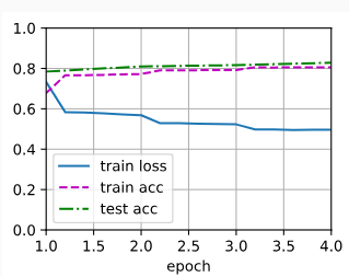

16.5.2.4. Using the Model
Finally, define the prediction function to output the logical relationship between a pair of premise and hypothesis.
마지막으로 전제 premise 와 가설 hypothesis 쌍의 논리적 관계를 출력하는 예측 함수를 정의합니다.
#@save
def predict_snli(net, vocab, premise, hypothesis):
    """Predict the logical relationship between the premise and hypothesis."""
    net.eval()
    premise = torch.tensor(vocab[premise], device=d2l.try_gpu())
    hypothesis = torch.tensor(vocab[hypothesis], device=d2l.try_gpu())
    label = torch.argmax(net([premise.reshape((1, -1)),
                           hypothesis.reshape((1, -1))]), dim=1)
    return 'entailment' if label == 0 else 'contradiction' if label == 1 \
            else 'neutral'
이 코드는 학습된 모델을 사용하여 주어진 전제(premise)와 가설(hypothesis) 사이의 논리적 관계를 예측하는 함수인 predict_snli를 정의합니다. 이 함수는 다음과 같은 작업을 수행합니다:
- net.eval(): 모델을 평가 모드로 설정합니다. 이것은 모델이 평가 모드에서 동작하도록 하며, 드롭아웃(dropout) 및 배치 정규화(batch normalization)와 같은 학습 중에만 필요한 연산들을 비활성화합니다.
- premise와 hypothesis: 전제와 가설은 텍스트 형식으로 주어지며, 이를 모델의 입력 형식에 맞게 변환합니다. 우선 vocab을 사용하여 텍스트를 토큰으로 변환하고, 그 다음에는 torch.tensor를 사용하여 텐서 형식으로 변환합니다. 이때, d2l.try_gpu()를 사용하여 가능한 경우 GPU 디바이스에 텐서를 할당합니다.
- net([premise.reshape((1, -1)), hypothesis.reshape((1, -1))]): 모델에 입력 데이터를 전달하여 논리적 관계를 예측합니다. 입력은 전제와 가설을 포함하며, 모델의 입력 형식에 맞게 텐서를 조작하고 모델에 전달합니다.
- label = torch.argmax(...): 모델의 출력에서 가장 높은 확률을 가지는 클래스를 선택합니다. 이를 위해 torch.argmax 함수를 사용하고, dim=1을 설정하여 각 예제에 대한 예측 클래스를 선택합니다.
- 최종적으로 예측된 클래스에 따라 'entailment' (유추), 'contradiction' (모순), 또는 'neutral' (중립) 중 하나의 논리적 관계를 반환합니다.
이 함수를 사용하면 모델을 통해 주어진 전제와 가설의 논리적 관계를 예측할 수 있습니다.
We can use the trained model to obtain the natural language inference result for a sample pair of sentences.
훈련된 모델을 사용하여 샘플 문장 쌍에 대한 자연어 추론 결과를 얻을 수 있습니다.
predict_snli(net, vocab, ['he', 'is', 'good', '.'], ['he', 'is', 'bad', '.'])이 코드는 predict_snli 함수를 사용하여 두 개의 문장(전제와 가설) 사이의 논리적 관계를 예측하는 예제입니다.
- net: 미리 학습된 모델로, 두 문장 사이의 논리적 관계를 예측하는 역할을 합니다.
- vocab: 어휘 사전으로, 모델이 텍스트를 이해하고 처리하는 데 사용됩니다.
- ['he', 'is', 'good', '.']: 첫 번째 문장인 전제를 토큰화한 리스트입니다. 여기서는 "he", "is", "good", "."로 구성되어 있습니다.
- ['he', 'is', 'bad', '.']: 두 번째 문장인 가설을 토큰화한 리스트입니다. 여기서는 "he", "is", "bad", "."로 구성되어 있습니다.
predict_snli 함수는 이 두 문장을 입력으로 받아 모델을 사용하여 논리적 관계를 예측하고, 예측된 결과를 반환합니다. 예를 들어, 이 코드를 실행하면 전제와 가설 사이의 관계를 예측하여 "entailment" (유추) 또는 "contradiction" (모순) 또는 "neutral" (중립) 중 하나의 결과를 반환할 것입니다.
'contradiction'

16.5.3. Summary
- The decomposable attention model consists of three steps for predicting the logical relationships between premises and hypotheses: attending, comparing, and aggregating.
분해 가능한 주의 모델은 전제와 가설 사이의 논리적 관계를 예측하기 위한 세 가지 단계(참석, 비교, 집계)로 구성됩니다. - With attention mechanisms, we can align tokens in one text sequence to every token in the other, and vice versa. Such alignment is soft using weighted average, where ideally large weights are associated with the tokens to be aligned.
주의 메커니즘을 사용하면 한 텍스트 시퀀스의 토큰을 다른 텍스트 시퀀스의 모든 토큰에 정렬하거나 그 반대로 정렬할 수 있습니다. 이러한 정렬은 가중 평균을 사용하여 소프트하게 이루어지며, 이상적으로는 큰 가중치가 정렬할 토큰과 연결됩니다. - The decomposition trick leads to a more desirable linear complexity than quadratic complexity when computing attention weights.
분해 트릭은 주의 가중치를 계산할 때 2차 복잡도보다 더 바람직한 선형 복잡도로 이어집니다. - We can use pretrained word vectors as the input representation for downstream natural language processing task such as natural language inference.
자연어 추론과 같은 다운스트림 자연어 처리 작업을 위한 입력 표현으로 사전 훈련된 단어 벡터를 사용할 수 있습니다.
16.5.4. Exercises
- Train the model with other combinations of hyperparameters. Can you get better accuracy on the test set?
- What are major drawbacks of the decomposable attention model for natural language inference?
- Suppose that we want to get the level of semantical similarity (e.g., a continuous value between 0 and 1) for any pair of sentences. How shall we collect and label the dataset? Can you design a model with attention mechanisms?
'Dive into Deep Learning > D2L Natural language Processing' 카테고리의 다른 글
| D2L - 16.7. Natural Language Inference: Fine-Tuning BERT (0) | 2023.09.02 |
|---|---|
| D2L - 16.6. Fine-Tuning BERT for Sequence-Level and Token-Level Applications (0) | 2023.09.02 |
| D2L - 16.4. Natural Language Inference and the Dataset (0) | 2023.09.01 |
| D2L - 16.3. Sentiment Analysis: Using Convolutional Neural Networks (0) | 2023.09.01 |
| D2L - 16.2. Sentiment Analysis: Using Recurrent Neural Networks (0) | 2023.09.01 |
| D2L - 16.1. Sentiment Analysis and the Dataset (0) | 2023.09.01 |
| D2L - 16. Natural Language Processing: Applications (0) | 2023.09.01 |
| D2L - 15.10. Pretraining BERT (0) | 2023.08.30 |
| D2L - 15.9. The Dataset for Pretraining BERT (0) | 2023.08.30 |
| D2L - 15.8. Bidirectional Encoder Representations from Transformers (BERT) (0) | 2023.08.30 |