반응형
블로그 이미지
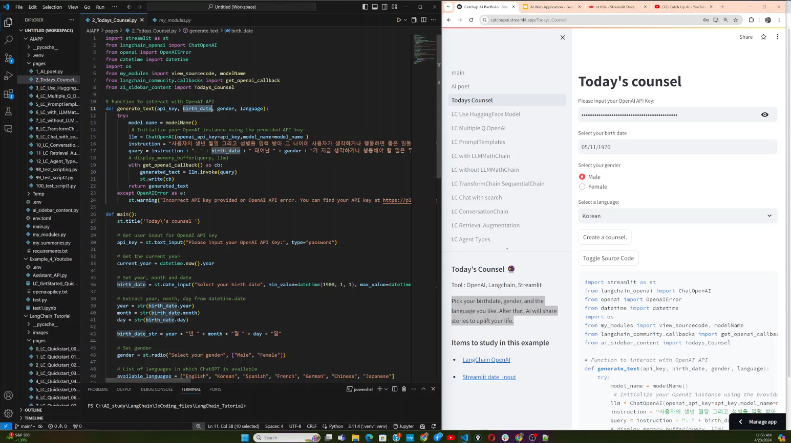
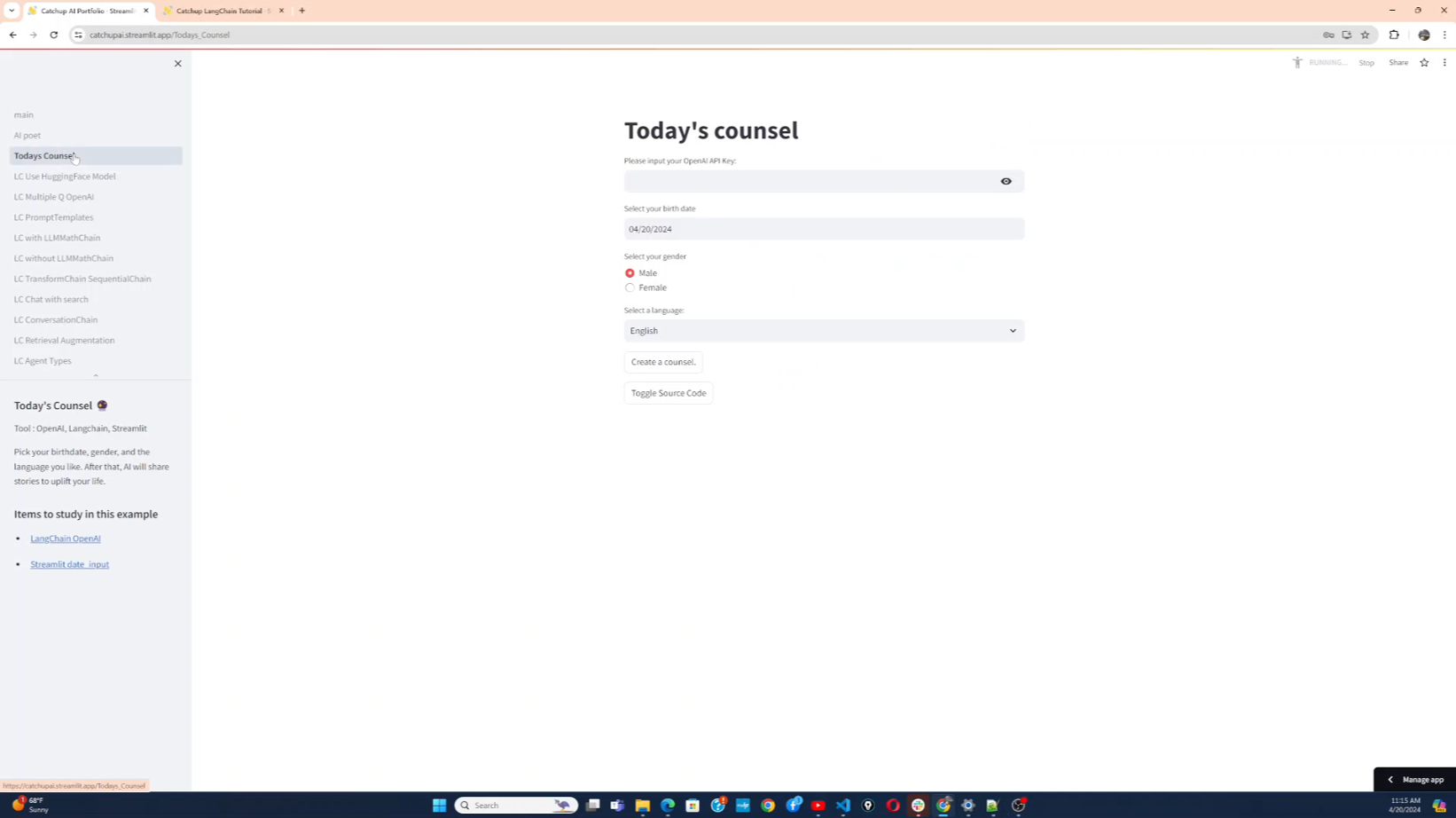
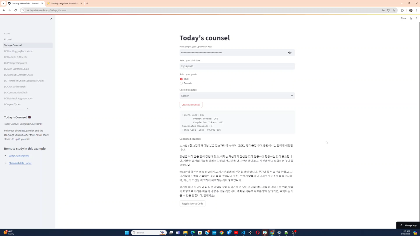
개발자로서 현장에서 일하면서 새로 접하는 기술들이나 알게된 정보 등을 정리하기 위한 블로그입니다. 운 좋게 미국에서 큰 회사들의 프로젝트에서 컬설턴트로 일하고 있어서 새로운 기술들을 접할 기회가 많이 있습니다. 미국의 IT 프로젝트에서 사용되는 툴들에 대해 많은 분들과 정보를 공유하고 싶습니다.
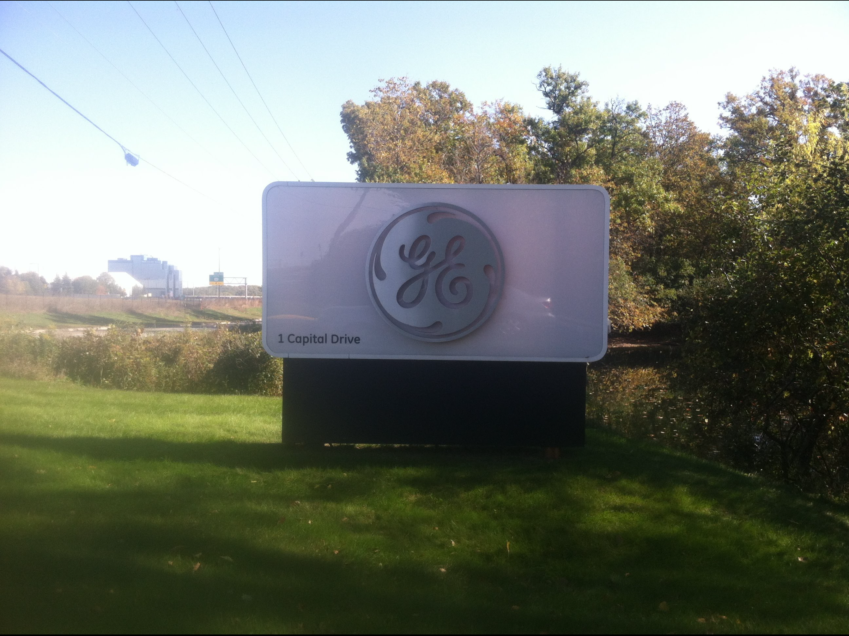
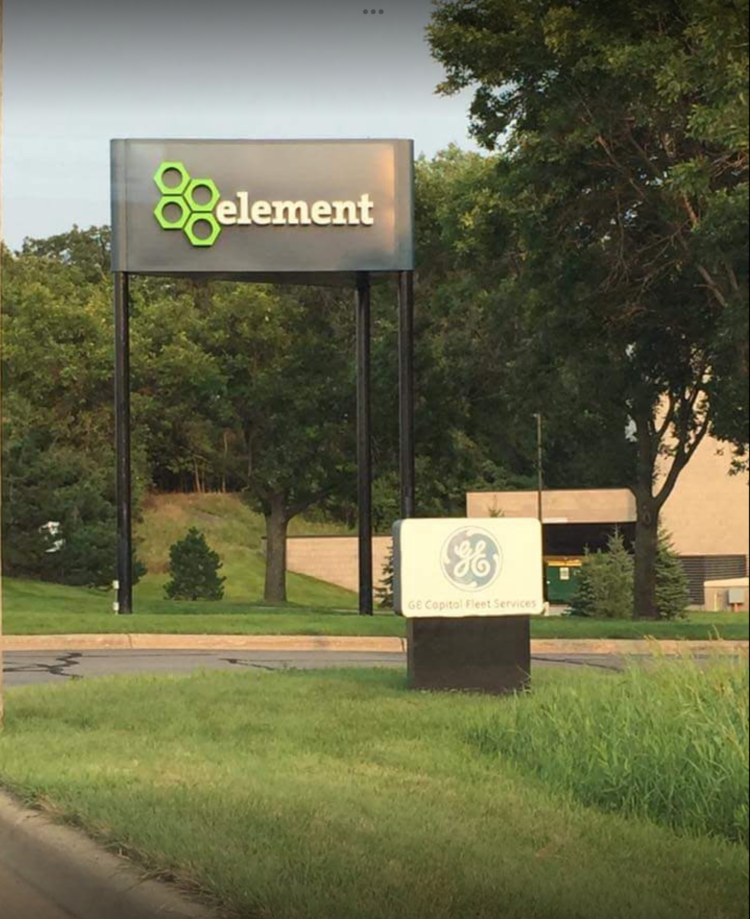
솔웅

최근에 올라온 글

최근에 달린 댓글

최근에 받은 트랙백

글 보관함

카테고리


반응형

https://huggingface.co/learn/nlp-course/chapter1/3?fw=pt


Transformers, what can they do? - Hugging Face NLP Course

In this section, we will look at what Transformer models can do and use our first tool from the 🤗 Transformers library: the pipeline() function. 👀 See that Open in Colab button on the top right? Click on it to open a Google Colab notebook with all th

huggingface.co


Transformers, what can they do?


In this section, we will look at what Transformer models can do and use our first tool from the 🤗 Transformers library: the pipeline() function.


이 섹션에서는 Transformer 모델이 수행할 수 있는 작업을 살펴보고 🤗 Transformers 라이브러리의 첫 번째 도구인 파이프라인() 함수를 사용합니다.


👀 See that Open in Colab button on the top right? Click on it to open a Google Colab notebook with all the code samples of this section. This button will be present in any section containing code examples.

If you want to run the examples locally, we recommend taking a look at the setup.


👀  오른쪽 상단에 Colab에서 열기 버튼이 보이시나요? 이 섹션의 모든 코드 샘플이 포함된 Google Colab 노트북을 열려면 클릭하세요. 이 버튼은 코드 예제가 포함된 모든 섹션에 표시됩니다.
예제를 로컬에서 실행하려면 설정을 살펴보는 것이 좋습니다.


Transformers are everywhere!

Transformer models are used to solve all kinds of NLP tasks, like the ones mentioned in the previous section. Here are some of the companies and organizations using Hugging Face and Transformer models, who also contribute back to the community by sharing their models:


Transformer 모델은 이전 섹션에서 언급한 것과 같은 모든 종류의 NLP 작업을 해결하는 데 사용됩니다. Hugging Face 및 Transformer 모델을 사용하고 모델을 공유하여 커뮤니티에 다시 기여하는 일부 회사 및 조직은 다음과 같습니다.


The 🤗 Transformers library provides the functionality to create and use those shared models. The Model Hub contains thousands of pretrained models that anyone can download and use. You can also upload your own models to the Hub!


🤗 Transformers 라이브러리는 이러한 공유 모델을 생성하고 사용할 수 있는 기능을 제공합니다. 모델 허브에는 누구나 다운로드하여 사용할 수 있는 수천 개의 사전 훈련된 모델이 포함되어 있습니다. 자신의 모델을 허브에 업로드할 수도 있습니다!


⚠️ The Hugging Face Hub is not limited to Transformer models. Anyone can share any kind of models or datasets they want! Create a huggingface.co account to benefit from all available features!

Before diving into how Transformer models work under the hood, let’s look at a few examples of how they can be used to solve some interesting NLP problems.


⚠️ Hugging Face Hub는 Transformer 모델에만 국한되지 않습니다. 누구나 원하는 모든 종류의 모델이나 데이터 세트를 공유할 수 있습니다! 사용 가능한 모든 기능을 활용하려면 Huggingface.co 계정을 만드세요!
Transformer 모델이 내부적으로 어떻게 작동하는지 알아보기 전에, 몇 가지 흥미로운 NLP 문제를 해결하는 데 어떻게 사용될 수 있는지에 대한 몇 가지 예를 살펴보겠습니다.


Working with pipelines


https://youtu.be/tiZFewofSLM?si=Es3SmFnc7IJSG0ts


The most basic object in the 🤗 Transformers library is the pipeline() function. It connects a model with its necessary preprocessing and postprocessing steps, allowing us to directly input any text and get an intelligible answer:


🤗 Transformers 라이브러리의 가장 기본적인 객체는 파이프라인() 함수입니다. 모델을 필요한 전처리 및 후처리 단계와 연결하여 텍스트를 직접 입력하고 이해하기 쉬운 답변을 얻을 수 있습니다.


from transformers import pipeline

classifier = pipeline("sentiment-analysis")
classifier("I've been waiting for a HuggingFace course my whole life.")


[{'label': 'POSITIVE', 'score': 0.9598047137260437}]


CoLab 실행 결과


We can even pass several sentences!


여러 문장을 전달할 수도 있습니다!


classifier(
    ["I've been waiting for a HuggingFace course my whole life.", "I hate this so much!"]
)


[{'label': 'POSITIVE', 'score': 0.9598047137260437},
 {'label': 'NEGATIVE', 'score': 0.9994558095932007}]


By default, this pipeline selects a particular pretrained model that has been fine-tuned for sentiment analysis in English. The model is downloaded and cached when you create the classifier object. If you rerun the command, the cached model will be used instead and there is no need to download the model again.


기본적으로 이 파이프라인은 영어로 된 감정 분석을 위해 미세 조정된 특정 사전 학습 모델을 선택합니다. 분류자 개체를 생성하면 모델이 다운로드되고 캐시됩니다. 명령을 다시 실행하면 캐시된 모델이 대신 사용되며 모델을 다시 다운로드할 필요가 없습니다.


There are three main steps involved when you pass some text to a pipeline:


일부 텍스트를 파이프라인에 전달할 때 관련된 세 가지 주요 단계는 다음과 같습니다.


  1. The text is preprocessed into a format the model can understand.
    텍스트는 모델이 이해할 수 있는 형식으로 전처리됩니다.
  2. The preprocessed inputs are passed to the model.
    전처리된 입력이 모델에 전달됩니다.
  3. The predictions of the model are post-processed, so you can make sense of them.
    모델의 예측은 사후 처리되므로 이를 이해할 수 있습니다.


Some of the currently available pipelines are:


현재 사용 가능한 파이프라인 중 일부는 다음과 같습니다.


  • feature-extraction (get the vector representation of a text)
  • fill-mask
  • ner (named entity recognition)
  • question-answering
  • sentiment-analysis
  • summarization
  • text-generation
  • translation
  • zero-shot-classification

Let’s have a look at a few of these!


이들 중 몇 가지를 살펴보겠습니다!


Zero-shot classification

We’ll start by tackling a more challenging task where we need to classify texts that haven’t been labelled. This is a common scenario in real-world projects because annotating text is usually time-consuming and requires domain expertise. For this use case, the zero-shot-classification pipeline is very powerful: it allows you to specify which labels to use for the classification, so you don’t have to rely on the labels of the pretrained model. You’ve already seen how the model can classify a sentence as positive or negative using those two labels — but it can also classify the text using any other set of labels you like.


라벨이 지정되지 않은 텍스트를 분류해야 하는 좀 더 어려운 작업부터 시작하겠습니다. 텍스트에 주석을 다는 것은 일반적으로 시간이 많이 걸리고 도메인 전문 지식이 필요하기 때문에 이는 실제 프로젝트에서 일반적인 시나리오입니다. 이 사용 사례의 경우 제로 샷 분류 파이프라인은 매우 강력합니다. 분류에 사용할 레이블을 지정할 수 있으므로 사전 훈련된 모델의 레이블에 의존할 필요가 없습니다. 모델이 두 레이블을 사용하여 문장을 긍정 또는 부정으로 분류하는 방법을 이미 확인했습니다. 하지만 원하는 다른 레이블 세트를 사용하여 텍스트를 분류할 수도 있습니다.


from transformers import pipeline

classifier = pipeline("zero-shot-classification")
classifier(
    "This is a course about the Transformers library",
    candidate_labels=["education", "politics", "business"],
)


{'sequence': 'This is a course about the Transformers library',
 'labels': ['education', 'business', 'politics'],
 'scores': [0.8445963859558105, 0.111976258456707, 0.043427448719739914]}


This pipeline is called zero-shot because you don’t need to fine-tune the model on your data to use it. It can directly return probability scores for any list of labels you want!


이 파이프라인을 사용하기 위해 데이터 모델을 미세 조정할 필요가 없기 때문에 제로샷이라고 합니다. 원하는 라벨 목록에 대한 확률 점수를 직접 반환할 수 있습니다!


✏️ Try it out! Play around with your own sequences and labels and see how the model behaves.


✏️ 한번 사용해 보세요! 자신만의 시퀀스와 라벨을 가지고 실험해보고 모델이 어떻게 작동하는지 확인하세요.


Text generation

Now let’s see how to use a pipeline to generate some text. The main idea here is that you provide a prompt and the model will auto-complete it by generating the remaining text. This is similar to the predictive text feature that is found on many phones. Text generation involves randomness, so it’s normal if you don’t get the same results as shown below.


이제 파이프라인을 사용하여 텍스트를 생성하는 방법을 살펴보겠습니다. 여기서 주요 아이디어는 프롬프트를 제공하면 모델이 나머지 텍스트를 생성하여 프롬프트를 자동 완성한다는 것입니다. 이는 많은 휴대폰에서 볼 수 있는 텍스트 예측 기능과 유사합니다. 텍스트 생성에는 무작위성이 포함되므로 아래와 같은 결과가 나오지 않는 것이 정상입니다.


from transformers import pipeline

generator = pipeline("text-generation")
generator("In this course, we will teach you how to")


[{'generated_text': 'In this course, we will teach you how to understand and use '
                    'data flow and data interchange when handling user data. We '
                    'will be working with one or more of the most commonly used '
                    'data flows — data flows of various types, as seen by the '
                    'HTTP'}]


You can control how many different sequences are generated with the argument num_return_sequences and the total length of the output text with the argument max_length.


num_return_sequences 인수를 사용하여 생성되는 서로 다른 시퀀스 수와 max_length 인수를 사용하여 출력 텍스트의 전체 길이를 제어할 수 있습니다.


✏️ Try it out! Use the num_return_sequences and max_length arguments to generate two sentences of 15 words each.


✏️ 한번 사용해 보세요! num_return_sequences 및 max_length 인수를 사용하여 각각 15개 단어로 구성된 두 문장을 생성합니다.


Using any model from the Hub in a pipeline

The previous examples used the default model for the task at hand, but you can also choose a particular model from the Hub to use in a pipeline for a specific task — say, text generation. Go to the Model Hub and click on the corresponding tag on the left to display only the supported models for that task. You should get to a page like this one.


이전 예제에서는 현재 작업에 기본 모델을 사용했지만 허브에서 특정 모델을 선택하여 특정 작업(예: 텍스트 생성)을 위한 파이프라인에서 사용할 수도 있습니다. 모델 허브로 이동하여 왼쪽에서 해당 태그를 클릭하면 해당 작업에 지원되는 모델만 표시됩니다. 이와 같은 페이지로 이동해야 합니다.


Let’s try the distilgpt2 model! Here’s how to load it in the same pipeline as before:


distilgpt2 모델을 사용해 봅시다! 이전과 동일한 파이프라인에서 이를 로드하는 방법은 다음과 같습니다.


from transformers import pipeline

generator = pipeline("text-generation", model="distilgpt2")
generator(
    "In this course, we will teach you how to",
    max_length=30,
    num_return_sequences=2,
)
[{'generated_text': 'In this course, we will teach you how to manipulate the world and '
                    'move your mental and physical capabilities to your advantage.'},
 {'generated_text': 'In this course, we will teach you how to become an expert and '
                    'practice realtime, and with a hands on experience on both real '
                    'time and real'}]


You can refine your search for a model by clicking on the language tags, and pick a model that will generate text in another language. The Model Hub even contains checkpoints for multilingual models that support several languages.


언어 태그를 클릭하여 모델 검색을 구체화하고 다른 언어로 텍스트를 생성할 모델을 선택할 수 있습니다. 모델 허브에는 여러 언어를 지원하는 다국어 모델에 대한 체크포인트도 포함되어 있습니다.


Once you select a model by clicking on it, you’ll see that there is a widget enabling you to try it directly online. This way you can quickly test the model’s capabilities before downloading it.


모델을 클릭하여 선택하면 온라인에서 직접 사용해 볼 수 있는 위젯이 표시됩니다. 이렇게 하면 모델을 다운로드하기 전에 모델의 기능을 빠르게 테스트할 수 있습니다.


✏️ Try it out! Use the filters to find a text generation model for another language. Feel free to play with the widget and use it in a pipeline!


✏️ 한번 사용해 보세요! 필터를 사용하여 다른 언어에 대한 텍스트 생성 모델을 찾으세요. 위젯을 자유롭게 가지고 파이프라인에서 사용해 보세요!


The Inference API

All the models can be tested directly through your browser using the Inference API, which is available on the Hugging Face website. You can play with the model directly on this page by inputting custom text and watching the model process the input data.


모든 모델은 Hugging Face 웹사이트에서 제공되는 Inference API를 사용하여 브라우저를 통해 직접 테스트할 수 있습니다. 이 페이지에서 사용자 정의 텍스트를 입력하고 모델이 입력 데이터를 처리하는 모습을 보면서 직접 모델을 가지고 놀 수 있습니다.


The Inference API that powers the widget is also available as a paid product, which comes in handy if you need it for your workflows. See the pricing page for more details.


위젯을 지원하는 Inference API는 유료 제품으로도 제공되므로 워크플로에 필요할 때 유용합니다. 자세한 내용은 가격 페이지를 참조하세요.


Mask filling

The next pipeline you’ll try is fill-mask. The idea of this task is to fill in the blanks in a given text:


시도할 다음 파이프라인은 채우기 마스크입니다. 이 작업의 아이디어는 주어진 텍스트의 빈칸을 채우는 것입니다.


from transformers import pipeline

unmasker = pipeline("fill-mask")
unmasker("This course will teach you all about <mask> models.", top_k=2)
[{'sequence': 'This course will teach you all about mathematical models.',
  'score': 0.19619831442832947,
  'token': 30412,
  'token_str': ' mathematical'},
 {'sequence': 'This course will teach you all about computational models.',
  'score': 0.04052725434303284,
  'token': 38163,
  'token_str': ' computational'}]


The top_k argument controls how many possibilities you want to be displayed. Note that here the model fills in the special <mask> word, which is often referred to as a mask token. Other mask-filling models might have different mask tokens, so it’s always good to verify the proper mask word when exploring other models. One way to check it is by looking at the mask word used in the widget.


top_k 인수는 표시할 가능성의 수를 제어합니다. 여기서 모델은 종종 마스크 토큰이라고 하는 특수 <mask> 단어를 채웁니다. 다른 마스크 채우기 모델에는 다른 마스크 토큰이 있을 수 있으므로 다른 모델을 탐색할 때 항상 적절한 마스크 단어를 확인하는 것이 좋습니다. 이를 확인하는 한 가지 방법은 위젯에 사용된 마스크 단어를 보는 것입니다.


✏️ Try it out! Search for the bert-base-cased model on the Hub and identify its mask word in the Inference API widget. What does this model predict for the sentence in our pipeline example above?


✏️ 한번 사용해 보세요! 허브에서 bert-base-cased 모델을 검색하고 Inference API 위젯에서 해당 마스크 단어를 식별합니다. 이 모델은 위 파이프라인 예의 문장에 대해 무엇을 예측합니까?


Named entity recognition


Named entity recognition (NER) is a task where the model has to find which parts of the input text correspond to entities such as persons, locations, or organizations. Let’s look at an example:


명명된 엔터티 인식(NER)은 모델이 입력 텍스트의 어느 부분이 사람, 위치 또는 조직과 같은 엔터티에 해당하는지 찾아야 하는 작업입니다. 예를 살펴보겠습니다:


from transformers import pipeline

ner = pipeline("ner", grouped_entities=True)
ner("My name is Sylvain and I work at Hugging Face in Brooklyn.")
[{'entity_group': 'PER', 'score': 0.99816, 'word': 'Sylvain', 'start': 11, 'end': 18}, 
 {'entity_group': 'ORG', 'score': 0.97960, 'word': 'Hugging Face', 'start': 33, 'end': 45}, 
 {'entity_group': 'LOC', 'score': 0.99321, 'word': 'Brooklyn', 'start': 49, 'end': 57}
]


Here the model correctly identified that Sylvain is a person (PER), Hugging Face an organization (ORG), and Brooklyn a location (LOC).


여기서 모델은 Sylvain이 사람(PER), Hugging Face가 조직(ORG), Brooklyn이 위치(LOC)임을 올바르게 식별했습니다.


We pass the option grouped_entities=True in the pipeline creation function to tell the pipeline to regroup together the parts of the sentence that correspond to the same entity: here the model correctly grouped “Hugging” and “Face” as a single organization, even though the name consists of multiple words. In fact, as we will see in the next chapter, the preprocessing even splits some words into smaller parts. For instance, Sylvain is split into four pieces: S, ##yl, ##va, and ##in. In the post-processing step, the pipeline successfully regrouped those pieces.


파이프라인 생성 함수에 grouped_entities=True 옵션을 전달하여 동일한 엔터티에 해당하는 문장 부분을 함께 재그룹화하도록 파이프라인에 지시합니다. 여기서 모델은 "Hugging"과 "Face"를 단일 조직으로 올바르게 그룹화했습니다. 이름은 여러 단어로 구성됩니다. 실제로 다음 장에서 살펴보겠지만 전처리는 일부 단어를 더 작은 부분으로 분할하기도 합니다. 예를 들어 Sylvain은 S, ##yl, ##va, ##in의 네 부분으로 나뉩니다. 사후 처리 단계에서 파이프라인은 해당 조각을 성공적으로 재그룹화했습니다.


✏️ Try it out! Search the Model Hub for a model able to do part-of-speech tagging (usually abbreviated as POS) in English. What does this model predict for the sentence in the example above?


✏️ 한번 사용해 보세요! 영어로 품사 태깅(보통 POS로 약칭)을 수행할 수 있는 모델을 모델 허브에서 검색하세요. 이 모델은 위 예의 문장에 대해 무엇을 예측합니까?


Question answering

The question-answering pipeline answers questions using information from a given context:


질문 답변 파이프라인은 주어진 컨텍스트의 정보를 사용하여 질문에 답변합니다.


from transformers import pipeline

question_answerer = pipeline("question-answering")
question_answerer(
    question="Where do I work?",
    context="My name is Sylvain and I work at Hugging Face in Brooklyn",
)
{'score': 0.6385916471481323, 'start': 33, 'end': 45, 'answer': 'Hugging Face'}


Note that this pipeline works by extracting information from the provided context; it does not generate the answer.


이 파이프라인은 제공된 컨텍스트에서 정보를 추출하여 작동합니다. 답변을 생성하지 않습니다.


Summarization

Summarization is the task of reducing a text into a shorter text while keeping all (or most) of the important aspects referenced in the text. Here’s an example:


요약은 텍스트에서 참조된 모든 중요한 측면을 유지하면서 텍스트를 더 짧은 텍스트로 줄이는 작업입니다. 예는 다음과 같습니다.


from transformers import pipeline

summarizer = pipeline("summarization")
summarizer(
    """
    America has changed dramatically during recent years. Not only has the number of 
    graduates in traditional engineering disciplines such as mechanical, civil, 
    electrical, chemical, and aeronautical engineering declined, but in most of 
    the premier American universities engineering curricula now concentrate on 
    and encourage largely the study of engineering science. As a result, there 
    are declining offerings in engineering subjects dealing with infrastructure, 
    the environment, and related issues, and greater concentration on high 
    technology subjects, largely supporting increasingly complex scientific 
    developments. While the latter is important, it should not be at the expense 
    of more traditional engineering.

    Rapidly developing economies such as China and India, as well as other 
    industrial countries in Europe and Asia, continue to encourage and advance 
    the teaching of engineering. Both China and India, respectively, graduate 
    six and eight times as many traditional engineers as does the United States. 
    Other industrial countries at minimum maintain their output, while America 
    suffers an increasingly serious decline in the number of engineering graduates 
    and a lack of well-educated engineers.
"""
)


[{'summary_text': ' America has changed dramatically during recent years . The '
                  'number of engineering graduates in the U.S. has declined in '
                  'traditional engineering disciplines such as mechanical, civil '
                  ', electrical, chemical, and aeronautical engineering . Rapidly '
                  'developing economies such as China and India, as well as other '
                  'industrial countries in Europe and Asia, continue to encourage '
                  'and advance engineering .'}]


Like with text generation, you can specify a max_length or a min_length for the result.


텍스트 생성과 마찬가지로 결과에 대해 max_length 또는 min_length를 지정할 수 있습니다.


Translation

For translation, you can use a default model if you provide a language pair in the task name (such as "translation_en_to_fr"), but the easiest way is to pick the model you want to use on the Model Hub. Here we’ll try translating from French to English:


번역의 경우 작업 이름에 언어 쌍(예: "translation_en_to_fr")을 제공하면 기본 모델을 사용할 수 있지만 가장 쉬운 방법은 모델 허브에서 사용하려는 모델을 선택하는 것입니다. 여기서는 프랑스어를 영어로 번역해 보겠습니다.


from transformers import pipeline

translator = pipeline("translation", model="Helsinki-NLP/opus-mt-fr-en")
translator("Ce cours est produit par Hugging Face.")
[{'translation_text': 'This course is produced by Hugging Face.'}]


한국어를 프랑스어로 번역할 경우


한국어를 영어로 번역할 경우.


Like with text generation and summarization, you can specify a max_length or a min_length for the result.


텍스트 생성 및 요약과 마찬가지로 결과에 대해 max_length 또는 min_length를 지정할 수 있습니다.


✏️ Try it out! Search for translation models in other languages and try to translate the previous sentence into a few different languages.


✏️ 한번 사용해 보세요! 다른 언어의 번역 모델을 검색하고 이전 문장을 몇 가지 다른 언어로 번역해 보세요.


The pipelines shown so far are mostly for demonstrative purposes. They were programmed for specific tasks and cannot perform variations of them. In the next chapter, you’ll learn what’s inside a pipeline() function and how to customize its behavior.


지금까지 표시된 파이프라인은 대부분 시연 목적으로 사용되었습니다. 특정 작업을 위해 프로그래밍되었으며 다양한 작업을 수행할 수 없습니다. 다음 장에서는 파이프라인() 함수 내부의 내용과 해당 동작을 사용자 정의하는 방법을 배우게 됩니다.


https://youtu.be/xbQ0DIJA0Bc?si=GhoIMvUzzRWJMFb9


반응형


반응형

https://huggingface.co/learn/nlp-course/chapter1/2?fw=pt


Natural Language Processing - Hugging Face NLP Course

2. Using 🤗 Transformers 3. Fine-tuning a pretrained model 4. Sharing models and tokenizers 5. The 🤗 Datasets library 6. The 🤗 Tokenizers library 9. Building and sharing demos new

huggingface.co


Before jumping into Transformer models, let’s do a quick overview of what natural language processing is and why we care about it.


Transformer 모델을 살펴보기 전에 자연어 처리가 무엇인지, 그리고 우리가 그것에 관심을 갖는 이유에 대해 간략하게 살펴보겠습니다.


What is NLP?

NLP is a field of linguistics and machine learning focused on understanding everything related to human language. The aim of NLP tasks is not only to understand single words individually, but to be able to understand the context of those words.


NLP는 인간 언어와 관련된 모든 것을 이해하는 데 초점을 맞춘 언어학 및 기계 학습 분야입니다. NLP 작업의 목표는 단일 단어를 개별적으로 이해하는 것뿐만 아니라 해당 단어의 맥락을 이해하는 것입니다.


The following is a list of common NLP tasks, with some examples of each:


다음은 일반적인 NLP 작업 목록과 각 작업의 몇 가지 예입니다.


  • Classifying whole sentences: Getting the sentiment of a review, detecting if an email is spam, determining if a sentence is grammatically correct or whether two sentences are logically related or not

  • 전체 문장 분류: 리뷰의 감정 파악, 이메일 스팸 여부 감지, 문장이 문법적으로 올바른지 또는 두 문장이 논리적으로 관련되어 있는지 확인

  • Classifying each word in a sentence: Identifying the grammatical components of a sentence (noun, verb, adjective), or the named entities (person, location, organization)

  • 문장의 각 단어 분류: 문장의 문법적 구성 요소(명사, 동사, 형용사) 또는 명명된 개체(사람, 위치, 조직) 식별

  • Generating text content: Completing a prompt with auto-generated text, filling in the blanks in a text with masked words

  • 텍스트 콘텐츠 생성: 자동 생성된 텍스트로 프롬프트 완성, 마스크된 단어로 텍스트의 공백 채우기

  • Extracting an answer from a text: Given a question and a context, extracting the answer to the question based on the information provided in the context

  • 텍스트에서 답변 추출: 질문과 컨텍스트가 주어지면, 컨텍스트에 제공된 정보를 기반으로 질문에 대한 답변을 추출합니다.

  • Generating a new sentence from an input text: Translating a text into another language, summarizing a text

  • 입력 텍스트에서 새 문장 생성: 텍스트를 다른 언어로 번역, 텍스트 요약


NLP isn’t limited to written text though. It also tackles complex challenges in speech recognition and computer vision, such as generating a transcript of an audio sample or a description of an image.


NLP는 서면 텍스트에만 국한되지 않습니다. 또한 오디오 샘플의 대본이나 이미지 설명 생성과 같은 음성 인식 및 컴퓨터 비전의 복잡한 문제를 해결합니다.


Why is it challenging? 왜 이것이 어려운가?


Computers don’t process information in the same way as humans. For example, when we read the sentence “I am hungry,” we can easily understand its meaning. Similarly, given two sentences such as “I am hungry” and “I am sad,” we’re able to easily determine how similar they are. For machine learning (ML) models, such tasks are more difficult. The text needs to be processed in a way that enables the model to learn from it. And because language is complex, we need to think carefully about how this processing must be done. There has been a lot of research done on how to represent text, and we will look at some methods in the next chapter.


컴퓨터는 인간과 같은 방식으로 정보를 처리하지 않습니다. 예를 들어, 우리는 “나는 배고프다”라는 문장을 읽으면 그 의미를 쉽게 이해할 수 있습니다. 마찬가지로, “나는 배고프다”와 “나는 슬프다”라는 두 문장이 주어지면 우리는 그 두 문장이 얼마나 비슷한지 쉽게 판단할 수 있습니다. 기계 학습(ML) 모델의 경우 이러한 작업은 더 어렵습니다. 텍스트는 모델이 학습할 수 있는 방식으로 처리되어야 합니다. 그리고 언어는 복잡하기 때문에 이 처리가 어떻게 이루어져야 하는지 신중하게 생각해야 합니다. 텍스트를 표현하는 방법에 대해 많은 연구가 진행되어 왔으며 다음 장에서 몇 가지 방법을 살펴보겠습니다.


반응형

The Hugging Face Course

2023. 12. 19. 13:35 | Posted by 솔웅


반응형

https://github.com/huggingface/course#translating-the-course-into-your-language


GitHub - huggingface/course: The Hugging Face course on Transformers

The Hugging Face course on Transformers. Contribute to huggingface/course development by creating an account on GitHub.

github.com


The Hugging Face Course


This repo contains the content that's used to create the Hugging Face course. The course teaches you about applying Transformers to various tasks in natural language processing and beyond. Along the way, you'll learn how to use the Hugging Face ecosystem — 🤗 Transformers, 🤗 Datasets, 🤗 Tokenizers, and 🤗 Accelerate — as well as the Hugging Face Hub. It's completely free and open-source!


이 저장소에는 Hugging Face 코스를 만드는 데 사용되는 콘텐츠가 포함되어 있습니다. 이 과정에서는 자연어 처리 및 그 이상의 다양한 작업에 Transformer를 적용하는 방법을 배웁니다. 그 과정에서 Hugging Face 생태계( 🤗 Transformers, 🤗 Datasets, 🤗 Tokenizers 및 🤗 Accelerate)와 Hugging Face Hub를 사용하는 방법을 배우게 됩니다. 완전 무료이며 오픈 소스입니다!


Translating the course into your language

As part of our mission to democratise machine learning, we'd love to have the course available in many more languages! Please follow the steps below if you'd like to help translate the course into your language 🙏.


기계 학습의 민주화를 위한 사명의 일환으로 우리는 이 과정을 더 많은 언어로 제공하고자 합니다! 강좌를 귀하의 언어로 번역하는 데 도움을 주고 싶으시다면 아래 단계를 따르세요 🙏.


🗞️ Open an issue


To get started, navigate to the Issues page of this repo and check if anyone else has opened an issue for your language. If not, open a new issue by selecting the Translation template from the New issue button.


시작하려면 이 저장소의 이슈 페이지로 이동하여 다른 사람이 귀하의 언어에 대한 이슈를 열었는지 확인하세요. 그렇지 않은 경우 새 이슈 버튼에서 번역 템플릿을 선택하여 새 이슈를 엽니다.


Once an issue is created, post a comment to indicate which chapters you'd like to work on and we'll add your name to the list.


이슈가 생성되면 작업하고 싶은 장을 나타내는 댓글을 게시하세요. 그러면 귀하의 이름이 목록에 추가됩니다.


🗣 Join our Discord

Since it can be difficult to discuss translation details quickly over GitHub issues, we have created dedicated channels for each language on our Discord server. If you'd like to join, follow the instructions at this channel 👉: https://discord.gg/JfAtkvEtRb


Join the Hugging Face Discord Server!

We're working to democratize good machine learning 🤗Join us! hf.co/jobs | 63782 members

discord.com


GitHub 문제로 인해 번역 세부 사항을 빠르게 논의하기 어려울 수 있으므로 Discord 서버에 언어별 전용 채널을 만들었습니다. 참여하고 싶다면 이 채널의 지침을 따르세요 👉: https://discord.gg/JfAtkvEtRb


🍴 Fork the repository

Next, you'll need to fork this repo. You can do this by clicking on the Fork button on the top-right corner of this repo's page.


다음으로 이 저장소를 포크해야 합니다. 이 저장소 페이지의 오른쪽 상단에 있는 Fork 버튼을 클릭하면 됩니다.


Once you've forked the repo, you'll want to get the files on your local machine for editing. You can do that by cloning the fork with Git as follows:


저장소를 포크한 후에는 편집을 위해 로컬 컴퓨터에 파일을 가져와야 합니다. 다음과 같이 Git으로 포크를 복제하면 됩니다.


git clone https://github.com/YOUR-USERNAME/course


📋 Copy-paste the English files with a new language code - 영어 파일을 새로운 언어 코드로 복사하여 붙여넣으세요.


The course files are organised under a main directory:


강좌 파일은 기본 디렉터리 아래에 구성되어 있습니다.


  • chapters: all the text and code snippets associated with the course.

  • chapters : 강좌와 관련된 모든 텍스트 및 코드 조각입니다.


You'll only need to copy the files in the chapters/en directory, so first navigate to your fork of the repo and run the following:


Chapters/en 디렉터리의 파일만 복사하면 되므로 먼저 저장소 포크로 이동하여 다음을 실행합니다.


cd ~/path/to/course
cp -r chapters/en/CHAPTER-NUMBER chapters/LANG-ID/CHAPTER-NUMBER


Here, CHAPTER-NUMBER refers to the chapter you'd like to work on and LANG-ID should be one of the ISO 639-1 or ISO 639-2 language codes -- see here for a handy table.


여기서 CHAPTER-NUMBER는 작업하려는 장을 나타내며 LANG-ID는 ISO 639-1 또는 ISO 639-2 언어 코드 중 하나여야 합니다. 편리한 표는 여기를 참조하세요.


Now comes the fun part - translating the text! The first thing we recommend is translating the part of the _toctree.yml file that corresponds to your chapter. This file is used to render the table of contents on the website and provide the links to the Colab notebooks. The only fields you should change are the title, ones -- for example, here are the parts of _toctree.yml that we'd translate for Chapter 0:


이제 재미있는 부분이 나옵니다. 바로 텍스트를 번역하는 것입니다! 우리가 권장하는 첫 번째 일은 귀하의 장에 해당하는 _toctree.yml 파일의 일부를 번역하는 것입니다. 이 파일은 웹사이트의 목차를 렌더링하고 Colab 노트북에 대한 링크를 제공하는 데 사용됩니다. 변경해야 할 유일한 필드는 제목입니다. 예를 들어, 다음은 0장에서 번역할 _toctree.yml 부분입니다.


- title: 0. Setup # Translate this!
  sections:
  - local: chapter0/1 # Do not change this!
    title: Introduction # Translate this!


🚨 Make sure the _toctree.yml file only contains the sections that have been translated! Otherwise you won't be able to build the content on the website or locally (see below how).

🚨 _toctree.yml 파일에 번역된 섹션만 포함되어 있는지 확인하세요! 그렇지 않으면 웹사이트나 로컬에서 콘텐츠를 구축할 수 없습니다(아래 방법 참조).

Once you have translated the _toctree.yml file, you can start translating the MDX files associated with your chapter.


_toctree.yml 파일을 번역한 후에는 해당 장과 관련된 MDX 파일 번역을 시작할 수 있습니다.


🙋 If the _toctree.yml file doesn't yet exist for your language, you can simply create one by copy-pasting from the English version and deleting the sections that aren't related to your chapter. Just make sure it exists in the chapters/LANG-ID/ directory!

🙋 해당 언어에 대한 _toctree.yml 파일이 아직 존재하지 않는 경우 영어 버전에서 복사하여 붙여넣고 해당 장과 관련 없는 섹션을 삭제하여 파일을 만들 수 있습니다. Chapters/LANG-ID/ 디렉토리에 있는지 확인하세요!

👷‍♂️ Build the course locally


Once you're happy with your changes, you can preview how they'll look by first installing the doc-builder tool that we use for building all documentation at Hugging Face:


변경 사항이 만족스러우면 먼저 Hugging Face에서 모든 문서를 작성하는 데 사용하는 문서 작성 도구를 설치하여 변경 사항이 어떻게 보일지 미리 볼 수 있습니다.


pip install hf-doc-builder


doc-builder preview course ../course/chapters/LANG-ID --not_python_module


**preview command does not work with Windows.


**미리보기 명령은 Windows에서 작동하지 않습니다.


This will build and render the course on http://localhost:3000/. Although the content looks much nicer on the Hugging Face website, this step will still allow you to check that everything is formatted correctly.


그러면 http://localhost:3000/에 강좌가 빌드되고 렌더링됩니다. Hugging Face 웹사이트의 콘텐츠가 훨씬 더 좋아 보이지만 이 단계를 통해 모든 항목의 형식이 올바른지 확인할 수 있습니다.


🚀 Submit a pull request


If the translations look good locally, the final step is to prepare the content for a pull request. Here, the first think to check is that the files are formatted correctly. For that you can run:


번역이 로컬에서 좋아 보인다면 마지막 단계는 끌어오기 요청을 위한 콘텐츠를 준비하는 것입니다. 여기서 가장 먼저 확인해야 할 점은 파일 형식이 올바른지 확인하는 것입니다. 이를 위해 다음을 실행할 수 있습니다.


pip install -r requirements.txt
make style


Once that's run, commit any changes, open a pull request, and tag @lewtun for a review. Congratulations, you've now completed your first translation 🥳!


실행이 완료되면 변경 사항을 커밋하고 끌어오기 요청을 열고 검토를 위해 @lewtun에 태그를 지정하세요. 축하합니다. 이제 첫 번째 번역이 완료되었습니다 🥳!


🚨 To build the course on the website, double-check your language code exists in languages field of the build_documentation.yml and build_pr_documentation.yml files in the .github folder. If not, just add them in their alphabetical order.

🚨 웹사이트에서 코스를 구축하려면 .github 폴더에 있는 build_documentation.yml 및 build_pr_documentation.yml 파일의 언어 필드에 언어 코드가 있는지 다시 확인하세요. 그렇지 않은 경우 알파벳 순서로 추가하세요.


📔 Jupyter notebooks

The Jupyter notebooks containing all the code from the course are hosted on the huggingface/notebooks repo. If you wish to generate them locally, first install the required dependencies:


강좌의 모든 코드가 포함된 Jupyter Notebook은 Huggingface/Notebooks 저장소에서 호스팅됩니다. 로컬로 생성하려면 먼저 필요한 종속성을 설치하십시오.


python -m pip install -r requirements.txt


Then run the following script: 그런 다음 다음 스크립트를 실행합니다.


python utils/generate_notebooks.py --output_dir nbs


This script extracts all the code snippets from the chapters and stores them as notebooks in the nbs folder (which is ignored by Git by default).


이 스크립트는 장에서 모든 코드 조각을 추출하여 nbs 폴더에 노트북으로 저장합니다(기본적으로 Git에서는 무시됩니다).


✍️ Contributing a new chapter

Note: we are not currently accepting community contributions for new chapters. These instructions are for the Hugging Face authors.

참고: 현재 새로운 챕터에 대한 커뮤니티 기여는 허용되지 않습니다. 이 지침은 Hugging Face 작성자를 위한 것입니다.

Adding a new chapter to the course is quite simple: 과정에 새 장을 추가하는 것은 매우 간단합니다.

  1. Create a new directory under chapters/en/chapterX, where chapterX is the chapter you'd like to add.

    Chapters/en/chapterX 아래에 새 디렉터리를 만듭니다. 여기서 ChapterX는 추가하려는 장입니다.

  2. Add numbered MDX files sectionX.mdx for each section. If you need to include images, place them in the huggingface-course/documentation-images repository and use the HTML Images Syntax with the path https://huggingface.co/datasets/huggingface-course/documentation-images/resolve/main/{langY}/{chapterX}/{your-image.png}.

    각 섹션에 대해 번호가 매겨진 MDX 파일 sectionX.mdx를 추가합니다. 이미지를 포함해야 하는 경우 해당 이미지를 Huggingface-course/documentation-images 저장소에 배치하고 https://huggingface.co/datasets/huggingface-course/documentation-images/resolve/main/ 경로와 함께 HTML 이미지 구문을 사용하세요. {langY}/{chapterX}/{your-image.png}.

  3. Update the _toctree.yml file to include your chapter sections -- this information will render the table of contents on the website. If your section involves both the PyTorch and TensorFlow APIs of transformers, make sure you include links to both Colabs in the colab field.

    장 섹션을 포함하도록 _toctree.yml 파일을 업데이트하세요. 이 정보는 웹 사이트의 목차를 렌더링합니다. 섹션에 변환기의 PyTorch 및 TensorFlow API가 모두 포함되어 있는 경우 colab 필드에 두 Colab에 대한 링크를 포함해야 합니다.

If you get stuck, check out one of the existing chapters -- this will often show you the expected syntax.


문제가 발생하면 기존 장 중 하나를 확인하세요. 예상되는 구문이 표시되는 경우가 많습니다.


Once you are happy with the content, open a pull request and tag @lewtun for a review. We recommend adding the first chapter draft as a single pull request -- the team will then provide feedback internally to iterate on the content 🤗!


콘텐츠가 만족스러우면 풀 요청을 열고 검토를 위해 @lewtun을 태그하세요. 단일 끌어오기 요청으로 첫 번째 장 초안을 추가하는 것이 좋습니다. 그런 다음 팀은 콘텐츠를 반복하기 위해 내부적으로 피드백을 제공합니다 🤗!


반응형

HF-NLP-Transformer models : Introduction

2023. 12. 19. 13:21 | Posted by 솔웅


반응형

https://huggingface.co/learn/nlp-course/chapter1/1?fw=pt


Introduction - Hugging Face NLP Course

2. Using 🤗 Transformers 3. Fine-tuning a pretrained model 4. Sharing models and tokenizers 5. The 🤗 Datasets library 6. The 🤗 Tokenizers library 9. Building and sharing demos new

huggingface.co


Introduction


Welcome to the 🤗 Course!


https://youtu.be/00GKzGyWFEs?si=_fwBMxuDBpygyJSj


This course will teach you about natural language processing (NLP) using libraries from the Hugging Face ecosystem — 🤗 Transformers, 🤗 Datasets, 🤗 Tokenizers, and 🤗 Accelerate — as well as the Hugging Face Hub. It’s completely free and without ads.


이 과정에서는 Hugging Face 생태계의 라이브러리( 🤗 Transformers, 🤗 Datasets, 🤗 Tokenizers 및 🤗 Accelerate)와 Hugging Face Hub를 사용하여 자연어 처리(NLP)에 대해 설명합니다. 완전 무료이며 광고도 없습니다.


What to expect?

Here is a brief overview of the course:


강좌에 대한 간략한 개요는 다음과 같습니다.


  • Chapters 1 to 4 provide an introduction to the main concepts of the 🤗 Transformers library. By the end of this part of the course, you will be familiar with how Transformer models work and will know how to use a model from the Hugging Face Hub, fine-tune it on a dataset, and share your results on the Hub!

  • 1장부터 4장까지는 🤗 Transformers 라이브러리의 주요 개념을 소개합니다. 과정의 이 부분이 끝나면 Transformer 모델의 작동 방식에 익숙해지고 Hugging Face Hub의 모델을 사용하는 방법, 데이터세트에서 이를 미세 조정하고 허브에서 결과를 공유하는 방법을 알게 됩니다!

  • Chapters 5 to 8 teach the basics of 🤗 Datasets and 🤗 Tokenizers before diving into classic NLP tasks. By the end of this part, you will be able to tackle the most common NLP problems by yourself.

  • 5~8장에서는 고전적인 NLP 작업을 시작하기 전에 🤗 데이터세트 및 🤗 토크나이저의 기본 사항을 가르칩니다. 이 부분이 끝나면 가장 일반적인 NLP 문제를 스스로 해결할 수 있게 됩니다.

  • Chapters 9 to 12 go beyond NLP, and explore how Transformer models can be used to tackle tasks in speech processing and computer vision. Along the way, you’ll learn how to build and share demos of your models, and optimize them for production environments. By the end of this part, you will be ready to apply 🤗 Transformers to (almost) any machine learning problem!

  • 9~12장에서는 NLP를 넘어 음성 처리 및 컴퓨터 비전 작업을 처리하는 데 Transformer 모델을 사용할 수 있는 방법을 살펴봅니다. 그 과정에서 모델의 데모를 구축 및 공유하고 생산 환경에 맞게 최적화하는 방법을 배우게 됩니다. 이 부분이 끝나면 🤗 Transformers를 (거의) 모든 기계 학습 문제에 적용할 수 있습니다!


This course: 이 과정

  • Requires a good knowledge of Python 
  • Python에 대한 충분한 지식이 필요합니다.

  • Is better taken after an introductory deep learning course, such as fast.ai’s Practical Deep Learning for Coders or one of the programs developed by DeepLearning.AI  
  • Does not expect prior PyTorch or TensorFlow knowledge, though some familiarity with either of those will help

  • fast.ai의 Practical Deep Learning for Coders 또는 DeepLearning.AI에서 개발한 프로그램 중 하나와 같은 입문 딥 러닝 과정을 수강하는 것이 좋습니다.

  • PyTorch 또는 TensorFlow에 대한 사전 지식을 기대하지 않지만 둘 중 하나에 익숙하면 도움이 됩니다.
 

Home

Learn the skills to start or advance your AI career | World-class education | Hands-on training | Collaborative community of peers and mentors

www.deeplearning.ai


After you’ve completed this course, we recommend checking out DeepLearning.AI’s Natural Language Processing Specialization, which covers a wide range of traditional NLP models like naive Bayes and LSTMs that are well worth knowing about!


이 과정을 마친 후에는 Naive Bayes 및 LSTM과 같이 알아 둘 가치가 있는 광범위한 기존 NLP 모델을 다루는 DeepLearning.AI의 자연어 처리 전문 분야를 확인하는 것이 좋습니다!


Who are we?

About the authors: 저자 소개


Abubakar Abid completed his PhD at Stanford in applied machine learning. During his PhD, he founded Gradio, an open-source Python library that has been used to build over 600,000 machine learning demos. Gradio was acquired by Hugging Face, which is where Abubakar now serves as a machine learning team lead.


Abubakar Abid는 스탠포드에서 응용 기계 학습 분야의 박사 학위를 취득했습니다. 박사 과정 동안 그는 600,000개 이상의 기계 학습 데모를 구축하는 데 사용된 오픈 소스 Python 라이브러리인 Gradio를 설립했습니다. Gradio는 현재 Abubakar가 기계 학습 팀 리더로 일하고 있는 Hugging Face에 인수되었습니다.


Matthew Carrigan is a Machine Learning Engineer at Hugging Face. He lives in Dublin, Ireland and previously worked as an ML engineer at Parse.ly and before that as a post-doctoral researcher at Trinity College Dublin. He does not believe we’re going to get to AGI by scaling existing architectures, but has high hopes for robot immortality regardless.


Matthew Carrigan은 Hugging Face의 머신러닝 엔지니어입니다. 그는 아일랜드 더블린에 거주하며 이전에는 Parse.ly에서 ML 엔지니어로 근무했고 그 전에는 Trinity College Dublin에서 박사후 연구원으로 근무했습니다. 그는 기존 아키텍처를 확장하는 것으로는  AGI에 도달할 것이라고 믿지 않지만 그럼에도 불구하고 로봇 불멸에 대한 높은 희망을 가지고 있습니다.


Lysandre Debut is a Machine Learning Engineer at Hugging Face and has been working on the 🤗 Transformers library since the very early development stages. His aim is to make NLP accessible for everyone by developing tools with a very simple API.


Lysandre Debut는 Hugging Face의 기계 학습 엔지니어이며 초기 개발 단계부터 🤗 Transformers 라이브러리 작업을 해왔습니다. 그의 목표는 매우 간단한 API로 도구를 개발하여 모든 사람이 NLP에 액세스할 수 있도록 하는 것입니다.


Sylvain Gugger is a Research Engineer at Hugging Face and one of the core maintainers of the 🤗 Transformers library. Previously he was a Research Scientist at fast.ai, and he co-wrote Deep Learning for Coders with fastai and PyTorch with Jeremy Howard. The main focus of his research is on making deep learning more accessible, by designing and improving techniques that allow models to train fast on limited resources.


Sylvain Gugger는 Hugging Face의 연구 엔지니어이자 🤗 Transformers 라이브러리의 핵심 관리자 중 한 명입니다. 이전에 그는 fast.ai의 연구 과학자였으며, fastai와 함께 Coders를 위한 Deep Learning, Jeremy Howard와 함께 PyTorch를 공동 집필했습니다. 그의 연구의 주요 초점은 모델이 제한된 리소스에서 빠르게 훈련할 수 있는 기술을 설계하고 개선하여 딥 러닝의 접근성을 높이는 것입니다.


Dawood Khan is a Machine Learning Engineer at Hugging Face. He’s from NYC and graduated from New York University studying Computer Science. After working as an iOS Engineer for a few years, Dawood quit to start Gradio with his fellow co-founders. Gradio was eventually acquired by Hugging Face.


Dawood Khan은 Hugging Face의 머신러닝 엔지니어입니다. 그는 뉴욕 출신이고 뉴욕 대학교에서 컴퓨터 공학을 전공했습니다. 몇 년 동안 iOS 엔지니어로 일한 후 Dawood는 동료 공동 창립자들과 함께 Gradio를 시작하기 위해 회사를 그만뒀습니다. Gradio는 결국 Hugging Face에 인수되었습니다.


Merve Noyan is a developer advocate at Hugging Face, working on developing tools and building content around them to democratize machine learning for everyone.


Merve Noyan은 Hugging Face의 개발자 옹호자로서 모든 사람을 위한 기계 학습을 민주화하기 위해 도구를 개발하고 관련 콘텐츠를 구축하는 작업을 하고 있습니다.


Lucile Saulnier is a machine learning engineer at Hugging Face, developing and supporting the use of open source tools. She is also actively involved in many research projects in the field of Natural Language Processing such as collaborative training and BigScience.


Lucile Saulnier는 Hugging Face의 머신 러닝 엔지니어로, 오픈 소스 도구 사용을 개발하고 지원합니다. 그녀는 또한 협업 훈련, BigScience 등 자연어 처리 분야의 많은 연구 프로젝트에 적극적으로 참여하고 있습니다.


Lewis Tunstall is a machine learning engineer at Hugging Face, focused on developing open-source tools and making them accessible to the wider community. He is also a co-author of the O’Reilly book Natural Language Processing with Transformers.


Lewis Tunstall은 Hugging Face의 기계 학습 엔지니어로, 오픈 소스 도구를 개발하고 이를 더 넓은 커뮤니티에 액세스할 수 있도록 하는 데 중점을 두고 있습니다. 그는 또한 O'Reilly의 책인 Transformers를 사용한 자연어 처리의 공동 저자이기도 합니다.


Leandro von Werra is a machine learning engineer in the open-source team at Hugging Face and also a co-author of the O’Reilly book Natural Language Processing with Transformers. He has several years of industry experience bringing NLP projects to production by working across the whole machine learning stack..


Leandro von Werra는 Hugging Face 오픈 소스 팀의 머신 러닝 엔지니어이자 O'Reilly의 Natural Language Process with Transformers 책의 공동 저자이기도 합니다. 그는 기계 학습 스택 전반에 걸쳐 NLP 프로젝트를 프로덕션으로 가져오는 수년간의 업계 경험을 보유하고 있습니다.


FAQ

Here are some answers to frequently asked questions:


자주 묻는 질문(FAQ)에 대한 답변은 다음과 같습니다.


  • Does taking this course lead to a certification? Currently we do not have any certification for this course. However, we are working on a certification program for the Hugging Face ecosystem — stay tuned!

  • 이 강좌를 수강하면 인증을 받을 수 있나요? 현재 이 과정에 대한 인증이 없습니다. 그러나 우리는 Hugging Face 생태계에 대한 인증 프로그램을 개발 중입니다. 계속 지켜봐 주시기 바랍니다!

  • How much time should I spend on this course? Each chapter in this course is designed to be completed in 1 week, with approximately 6-8 hours of work per week. However, you can take as much time as you need to complete the course.

  • 이 강좌에 얼마나 많은 시간을 투자해야 합니까? 이 과정의 각 장은 주당 약 6~8시간씩 1주일 내에 완료하도록 설계되었습니다. 그러나 과정을 완료하는 데 필요한 만큼의 시간을 투자할 수 있습니다.

  • Where can I ask a question if I have one? If you have a question about any section of the course, just click on the ”Ask a question” banner at the top of the page to be automatically redirected to the right section of the Hugging Face forums:

  • 질문이 있으면 어디로 문의해야 하나요? 코스의 특정 섹션에 대해 질문이 있는 경우 페이지 상단의 "질문하기" 배너를 클릭하면 자동으로 Hugging Face 포럼의 해당 섹션으로 리디렉션됩니다.


https://discuss.huggingface.co/t/chapter-1-questions


Chapter 1 questions

Use this topic for any question about Chapter 1 of the course.

discuss.huggingface.co


Note that a list of project ideas is also available on the forums if you wish to practice more once you have completed the course.


과정을 마친 후 더 연습하고 싶다면 포럼에서 프로젝트 아이디어 목록을 확인할 수도 있습니다.


  • Where can I get the code for the course? For each section, click on the banner at the top of the page to run the code in either Google Colab or Amazon SageMaker Studio Lab:

  • 강의 코드는 어디서 받을 수 있나요? 각 섹션에 대해 페이지 상단의 배너를 클릭하여 Google Colab 또는 Amazon SageMaker Studio Lab에서 코드를 실행하세요.


The Jupyter notebooks containing all the code from the course are hosted on the huggingface/notebooks repo. If you wish to generate them locally, check out the instructions in the course repo on GitHub.


강좌의 모든 코드가 포함된 Jupyter Notebook은 Huggingface/Notebooks 저장소에서 호스팅됩니다. 로컬에서 생성하려면 GitHub의 코스 저장소에 있는 지침을 확인하세요.


  • How can I contribute to the course? There are many ways to contribute to the course! If you find a typo or a bug, please open an issue on the course repo. If you would like to help translate the course into your native language, check out the instructions here.

  • 강좌에 어떻게 기여할 수 있나요? 강좌에 참여하는 방법에는 여러 가지가 있습니다! 오타나 버그를 발견한 경우 코스 저장소에서 문제를 열어주세요. 강좌를 모국어로 번역하는 데 도움을 주고 싶다면 여기에서 지침을 확인하세요.

  • What were the choices made for each translation? Each translation has a glossary and TRANSLATING.txt file that details the choices that were made for machine learning jargon etc. You can find an example for German here.

  • 각 번역에 대해 어떤 선택이 이루어졌나요? 각 번역에는 기계 학습 전문 용어 등에 대한 선택 사항을 자세히 설명하는 용어집과 TRANSLATING.txt 파일이 있습니다. 여기에서 독일어에 대한 예를 찾을 수 있습니다.
  • Can I reuse this course? Of course! The course is released under the permissive Apache 2 license. This means that you must give appropriate credit, provide a link to the license, and indicate if changes were made. You may do so in any reasonable manner, but not in any way that suggests the licensor endorses you or your use. If you would like to cite the course, please use the following BibTeX:

  • 이 강좌를 재사용할 수 있나요? 물론! 이 과정은 허용되는 Apache 2 라이센스에 따라 공개됩니다. 이는 적절한 출처를 표시하고 라이선스에 대한 링크를 제공하고 변경 사항이 있는지 표시해야 함을 의미합니다. 귀하는 합리적인 방식으로 그렇게 할 수 있지만, 라이센스 제공자가 귀하 또는 귀하의 사용을 보증하는 방식으로 그렇게 할 수는 없습니다. 강좌를 인용하려면 다음 BibTeX를 사용하세요.
@misc{huggingfacecourse,
  author = {Hugging Face},
  title = {The Hugging Face Course, 2022},
  howpublished = "\url{https://huggingface.co/course}",
  year = {2022},
  note = "[Online; accessed <today>]"
}


Let's Go

Are you ready to roll? In this chapter, you will learn:


굴릴 준비가 되셨나요? 이 장에서는 다음 내용을 학습합니다.

  • How to use the pipeline() function to solve NLP tasks such as text generation and classification

  • 파이프라인() 함수를 사용하여 텍스트 생성 및 분류와 같은 NLP 작업을 해결하는 방법

  • About the Transformer architecture

  • Transformer 아키텍처 정보

  • How to distinguish between encoder, decoder, and encoder-decoder architectures and use cases

  • 인코더, 디코더, 인코더-디코더 아키텍처와 사용 사례를 구별하는 방법


반응형

HF-NLP-Setup Introduction

2023. 12. 19. 05:11 | Posted by 솔웅


반응형

https://huggingface.co/learn/nlp-course/chapter0/1?fw=pt


Introduction - Hugging Face NLP Course

2. Using 🤗 Transformers 3. Fine-tuning a pretrained model 4. Sharing models and tokenizers 5. The 🤗 Datasets library 6. The 🤗 Tokenizers library 9. Building and sharing demos new

huggingface.co


Introduction


Welcome to the Hugging Face course! This introduction will guide you through setting up a working environment. If you’re just starting the course, we recommend you first take a look at Chapter 1, then come back and set up your environment so you can try the code yourself.


Hugging Face 코스에 오신 것을 환영합니다! 이 소개에서는 작업 환경을 설정하는 과정을 안내합니다. 과정을 막 시작하는 경우 먼저 1장을 살펴보고 다시 돌아와서 코드를 직접 사용해 볼 수 있도록 환경을 설정하는 것이 좋습니다.


All the libraries that we’ll be using in this course are available as Python packages, so here we’ll show you how to set up a Python environment and install the specific libraries you’ll need.


이 과정에서 사용할 모든 라이브러리는 Python 패키지로 제공되므로 여기서는 Python 환경을 설정하고 필요한 특정 라이브러리를 설치하는 방법을 보여 드리겠습니다.


We’ll cover two ways of setting up your working environment, using a Colab notebook or a Python virtual environment. Feel free to choose the one that resonates with you the most. For beginners, we strongly recommend that you get started by using a Colab notebook.


Colab 노트북이나 Python 가상 환경을 사용하여 작업 환경을 설정하는 두 가지 방법을 다루겠습니다. 당신에게 가장 공감되는 것을 자유롭게 선택하십시오. 초보자의 경우 Colab 노트북을 사용하여 시작하는 것이 좋습니다.


Note that we will not be covering the Windows system. If you’re running on Windows, we recommend following along using a Colab notebook. If you’re using a Linux distribution or macOS, you can use either approach described here.


Windows 시스템은 다루지 않습니다. Windows에서 실행하는 경우 Colab 노트북을 사용하여 따라하는 것이 좋습니다. Linux 배포판이나 macOS를 사용하는 경우 여기에 설명된 접근 방식 중 하나를 사용할 수 있습니다.


Most of the course relies on you having a Hugging Face account. We recommend creating one now: create an account.


대부분의 과정은 Hugging Face 계정이 있어야 합니다. 지금 계정을 만드는 것이 좋습니다. 계정을 만드세요.


Using a Google Colab notebook

Using a Colab notebook is the simplest possible setup; boot up a notebook in your browser and get straight to coding!


Colab 노트북을 사용하는 것이 가장 간단한 설정입니다. 브라우저에서 노트북을 부팅하고 바로 코딩을 시작해 보세요!


If you’re not familiar with Colab, we recommend you start by following the introduction. Colab allows you to use some accelerating hardware, like GPUs or TPUs, and it is free for smaller workloads.


Colab에 익숙하지 않다면 소개부터 시작하는 것이 좋습니다. Colab을 사용하면 GPU 또는 TPU와 같은 일부 가속 하드웨어를 사용할 수 있으며 소규모 워크로드에는 무료로 제공됩니다.


Once you’re comfortable moving around in Colab, create a new notebook and get started with the setup:


Colab에서 편안하게 이동하고 나면 새 노트북을 만들고 설정을 시작하세요.


The next step is to install the libraries that we’ll be using in this course. We’ll use pip for the installation, which is the package manager for Python. In notebooks, you can run system commands by preceding them with the ! character, so you can install the 🤗 Transformers library as follows:


다음 단계는 이 과정에서 사용할 라이브러리를 설치하는 것입니다. Python의 패키지 관리자인 pip를 설치에 사용하겠습니다. 노트북에서는 앞에 !를 붙여 시스템 명령을 실행할 수 있습니다. 캐릭터이므로 다음과 같이 🤗 Transformers 라이브러리를 설치할 수 있습니다.


!pip install transformers


You can make sure the package was correctly installed by importing it within your Python runtime:


Python 런타임 내에서 패키지를 가져와 패키지가 올바르게 설치되었는지 확인할 수 있습니다.


import transformers


This installs a very light version of 🤗 Transformers. In particular, no specific machine learning frameworks (like PyTorch or TensorFlow) are installed. Since we’ll be using a lot of different features of the library, we recommend installing the development version, which comes with all the required dependencies for pretty much any imaginable use case:


이것은 🤗 Transformers의 매우 가벼운 버전을 설치합니다. 특히, 특정 기계 학습 프레임워크(예: PyTorch 또는 TensorFlow)가 설치되지 않습니다. 우리는 라이브러리의 다양한 기능을 사용할 것이므로 상상할 수 있는 거의 모든 사용 사례에 필요한 모든 종속성이 포함된 개발 버전을 설치하는 것이 좋습니다.


!pip install transformers[sentencepiece]


This will take a bit of time, but then you’ll be ready to go for the rest of the course!


약간의 시간이 걸리겠지만, 그러면 나머지 과정을 진행할 준비가 된 것입니다!


Using a Python virtual environment

If you prefer to use a Python virtual environment, the first step is to install Python on your system. We recommend following this guide to get started.


Python 가상 환경을 사용하려는 경우 첫 번째 단계는 시스템에 Python을 설치하는 것입니다. 시작하려면 이 가이드를 따르는 것이 좋습니다.


Once you have Python installed, you should be able to run Python commands in your terminal. You can start by running the following command to ensure that it is correctly installed before proceeding to the next steps: python --version. This should print out the Python version now available on your system.


Python을 설치하고 나면 터미널에서 Python 명령을 실행할 수 있습니다. 다음 단계를 진행하기 전에 python --version 명령을 실행하여 올바르게 설치되었는지 확인할 수 있습니다. 그러면 현재 시스템에서 사용할 수 있는 Python 버전이 인쇄됩니다.


When running a Python command in your terminal, such as python --version, you should think of the program running your command as the “main” Python on your system. We recommend keeping this main installation free of any packages, and using it to create separate environments for each application you work on — this way, each application can have its own dependencies and packages, and you won’t need to worry about potential compatibility issues with other applications.


python --version과 같은 Python 명령을 터미널에서 실행할 때 명령을 실행하는 프로그램을 시스템의 "기본" Python으로 생각해야 합니다. 이 기본 설치에 패키지를 사용하지 않고 이를 사용하여 작업하는 각 애플리케이션에 대해 별도의 환경을 만드는 것이 좋습니다. 이렇게 하면 각 애플리케이션이 자체 종속성과 패키지를 가질 수 있습니다.다른 응용 프로그램과의 잠재적인 호환성 문제에 대해 걱정할 필요가 없습니다.


In Python this is done with virtual environments, which are self-contained directory trees that each contain a Python installation with a particular Python version alongside all the packages the application needs. Creating such a virtual environment can be done with a number of different tools, but we’ll use the official Python package for that purpose, which is called venv.


Python에서는 애플리케이션에 필요한 모든 패키지와 함께 특정 Python 버전이 포함된 Python 설치가 포함된 독립형 디렉터리 트리인 가상 환경을 통해 이 작업이 수행됩니다. 이러한 가상 환경을 만드는 것은 다양한 도구를 사용하여 수행할 수 있지만 우리는 해당 목적을 위해 venv라고 하는 공식 Python 패키지를 사용하겠습니다.


First, create the directory you’d like your application to live in — for example, you might want to make a new directory called transformers-course at the root of your home directory:


먼저, 애플리케이션을 보관할 디렉터리를 만듭니다. 예를 들어 홈 디렉터리의 루트에 Transformers-course라는 새 디렉터리를 만들 수 있습니다.


mkdir ~/transformers-course
cd ~/transformers-course


From inside this directory, create a virtual environment using the Python venv module:


이 디렉터리 내에서 Python venv 모듈을 사용하여 가상 환경을 만듭니다.


python -m venv .env


나는 윈도우 환경에서 실행하고 있으며 가상 환경 이름은 hfnlp라고 하겠음.


You should now have a directory called .env in your otherwise empty folder:


이제 빈 폴더에 .env라는 디렉터리가 있어야 합니다.


ls -a
.      ..    .env


내 윈도우 로컬 환경에서는 아래와 같이 dir로 디렉토리 내용을 볼 수 있음. hfnlp 폴더가 생성 돼 있음.


You can jump in and out of your virtual environment with the activate and deactivate scripts:


활성화 및 비활성화 스크립트를 사용하여 가상 환경에 들어가고 나올 수 있습니다.


# Activate the virtual environment
source .env/bin/activate

# Deactivate the virtual environment
source .env/bin/deactivate


윈도우에서는 Scripts라는 폴더에 있는 activate를 실행하면 됨


이 가상환경에서 나오려면 deactivate 하면 됨.


You can make sure that the environment is activated by running the which python command: if it points to the virtual environment, then you have successfully activated it!


which python 명령을 실행하여 환경이 활성화되었는지 확인할 수 있습니다. 가상 환경을 가리키면 성공적으로 활성화된 것입니다!


which python


/home/<user>/transformers-course/.env/bin/python


윈도우 환경에서는 비슷한 명령어로 where python이 있음.


Installing dependencies

As in the previous section on using Google Colab instances, you’ll now need to install the packages required to continue. Again, you can install the development version of 🤗 Transformers using the pip package manager:


Google Colab 인스턴스 사용에 대한 이전 섹션과 마찬가지로 이제 계속하려면 필요한 패키지를 설치해야 합니다. 이번에도 pip 패키지 관리자를 사용하여 🤗 Transformers의 개발 버전을 설치할 수 있습니다.


pip install "transformers[sentencepiece]"


You’re now all set up and ready to go!


이제 모든 설정이 완료되었으며 사용할 준비가 되었습니다!


반응형

Dec 14, 2023 Superalignment Fast Grants

2023. 12. 19. 03:45 | Posted by 솔웅


반응형

https://openai.com/blog/superalignment-fast-grants


Superalignment Fast Grants

We’re launching $10M in grants to support technical research towards the alignment and safety of superhuman AI systems, including weak-to-strong generalization, interpretability, scalable oversight, and more.

openai.com


Superalignment Fast Grants

We’re launching $10M in grants to support technical research towards the alignment and safety of superhuman AI systems, including weak-to-strong generalization, interpretability, scalable oversight, and more.


우리는 약-강 일반화, 해석 가능성, 확장 가능한 감독 등을 포함하여 초인적 AI 시스템의 정렬과 안전을 향한 기술 연구를 지원하기 위해 1,000만 달러의 보조금을 지급할 예정입니다.


We believe superintelligence could arrive within the next 10 years. These AI systems would have vast capabilities—they could be hugely beneficial, but also potentially pose large risks.


우리는 초지능이 앞으로 10년 안에 도래할 것이라고 믿습니다. 이러한 AI 시스템은 방대한 기능을 갖추고 있어 큰 이점을 제공할 수 있지만 잠재적으로 큰 위험을 초래할 수도 있습니다.


Today, we align AI systems to ensure they are safe using reinforcement learning from human feedback (RLHF). However, aligning future superhuman AI systems will pose fundamentally new and qualitatively different technical challenges. 


현재 우리는 인간 피드백(RLHF)을 통한 강화 학습을 사용하여 AI 시스템이 안전한지 확인하도록 조정합니다. 그러나 미래의 초인적 AI 시스템을 조정하는 것은 근본적으로 새롭고 질적으로 다른 기술적 과제를 제기할 것입니다.


Superhuman AI systems will be capable of complex and creative behaviors that humans cannot fully understand. For example, if a superhuman model generates a million lines of extremely complicated code, humans will not be able to reliably evaluate whether the code is safe or dangerous to execute. Existing alignment techniques like RLHF that rely on human supervision may no longer be sufficient. This leads to the fundamental challenge: how can humans steer and trust AI systems much smarter than them? 


초인적 AI 시스템은 인간이 완전히 이해할 수 없는 복잡하고 창의적인 행동을 수행할 수 있게 될 것입니다. 예를 들어, 초인적 모델이 수백만 줄의 극도로 복잡한 코드를 생성한다면 인간은 코드가 실행하기에 안전한지 아니면 위험한지 확실하게 평가할 수 없습니다. 사람의 감독에 의존하는 RLHF와 같은 기존 정렬 기술로는 더 이상 충분하지 않을 수 있습니다. 이는 근본적인 과제로 이어집니다. 인간이 어떻게 AI 시스템을 인간보다 훨씬 더 똑똑하게 조종하고 신뢰할 수 있습니까?


This is one of the most important unsolved technical problems in the world. But we think it is solvable with a concerted effort. There are many promising approaches and exciting directions, with lots of low-hanging fruit. We think there is an enormous opportunity for the ML research community and individual researchers to make major progress on this problem today. 


이는 세계에서 가장 중요한 미해결 기술 문제 중 하나입니다. 하지만 우리는 공동의 노력으로 이 문제를 해결할 수 있다고 생각합니다. 많은 유망한 접근 방식과 흥미로운 방향이 있으며, 쉽게 얻을 수 있는 성과도 많습니다. 우리는 오늘날 ML 연구 커뮤니티와 개별 연구자가 이 문제에 대해 큰 진전을 이룰 수 있는 엄청난 기회가 있다고 생각합니다.


As part of our Superalignment project, we want to rally the best researchers and engineers in the world to meet this challenge—and we’re especially excited to bring new people into the field.


Superalignment 프로젝트의 일환으로 우리는 이 과제를 해결하기 위해 세계 최고의 연구원과 엔지니어를 모으고 싶습니다. 특히 새로운 사람들을 현장에 데려오게 되어 기쁩니다.


Superalignment Fast Grants

In partnership with Eric Schmidt, we are launching a $10M grants program to support technical research towards ensuring superhuman AI systems are aligned and safe:


우리는 Eric Schmidt와 협력하여 초인적인 AI 시스템을 정렬하고 안전하게 유지하기 위한 기술 연구를 지원하기 위해 1,000만 달러의 보조금 프로그램을 시작합니다.


  • We are offering $100K–$2M grants for academic labs, nonprofits, and individual researchers.
  • 우리는 학술 연구실, 비영리 단체 및 개인 연구자에게 10만~200만 달러의 보조금을 제공하고 있습니다.
  • For graduate students, we are sponsoring a one-year $150K OpenAI Superalignment Fellowship: $75K in stipend and $75K in compute and research funding.
  • 대학원생을 위해 우리는 1년 동안 $150,000의 OpenAI Superalignment Fellowship을 후원합니다(급여 $75,000, 컴퓨팅 및 연구 자금 $75,000).
  • No prior experience working on alignment is required; we are actively looking to support researchers who are excited to work on alignment for the first time.
  • 정렬 작업에 대한 사전 경험은 필요하지 않습니다. 우리는 처음으로 정렬 작업을 하게 된 연구자들을 적극적으로 지원하기 위해 노력하고 있습니다.
  • Our application process is simple, and we’ll get back to you within four weeks of applications closing. 
  • 우리의 신청 절차는 간단하며, 신청 마감 후 4주 이내에 연락드리겠습니다.


With these grants, we are particularly interested in funding the following research directions:


이러한 보조금을 통해 우리는 특히 다음 연구 방향에 자금을 지원하는 데 관심이 있습니다.

  • Weak-to-strong generalization: Humans will be weak supervisors relative to superhuman models. Can we understand and control how strong models generalize from weak supervision
  • 약한 대 강한 일반화: 인간은 초인간 모델에 비해 약한 감독자가 될 것입니다. 약한 감독으로 인해 강력한 모델이 일반화되는 방식을 이해하고 제어할 수 있나요?
  • Interpretability: How can we understand model internals? And can we use this to e.g. build an AI lie detector?
  • 해석성: 모델 내부를 어떻게 이해할 수 있습니까? 그리고 이것을 다음과 같은 용도로 사용할 수 있습니까? AI 거짓말 탐지기를 만들까?
  • Scalable oversight: How can we use AI systems to assist humans in evaluating the outputs of other AI systems on complex tasks?
  • 확장 가능한 감독: 인간이 복잡한 작업에 대해 다른 AI 시스템의 결과를 평가할 수 있도록 AI 시스템을 어떻게 사용할 수 있습니까?
  • Many other research directions, including but not limited to: honesty, chain-of-thought faithfulness, adversarial robustness, evals and testbeds, and more.
  • 정직성, 사고방식의 충실성, 적대적 견고성, 평가 및 테스트베드 등을 포함하되 이에 국한되지 않는 다양한 연구 방향.


For more on the research directions, FAQs, and other details, see our Superalignment Fast Grants page.


연구 방향, FAQ 및 기타 세부 사항에 대한 자세한 내용은 Superalignment Fast Grants 페이지를 참조하세요.


Join us in this challenge

We think new researchers could make enormous contributions! This is a young field with many tractable research problems; outstanding contributions could not just help shape the field, but be critical for the future of AI. There has never been a better time to start working on alignment.


우리는 새로운 연구자들이 엄청난 기여를 할 수 있다고 생각합니다! 이것은 다루기 쉬운 연구 문제가 많은 젊은 분야입니다. 탁월한 기여는 해당 분야를 형성하는 데 도움이 될 뿐만 아니라 AI의 미래에 매우 중요합니다. 정렬 작업을 시작하기에 이보다 더 좋은 때는 없었습니다.


반응형


반응형

https://openai.com/blog/axel-springer-partnership


Partnership with Axel Springer to deepen beneficial use of AI in journalism

Axel Springer is the first publishing house globally to partner with us on a deeper integration of journalism in AI technologies.

openai.com


Partnership with Axel Springer to deepen beneficial use of AI in journalism                         

Axel Springer is the first publishing house globally to partner with us on a deeper integration of journalism in AI technologies.


This news was originally shared by Axel Springer and can also be read here.


이 소식은 원래 Axel Springer가 공유했으며 여기에서도 읽을 수 있습니다.


Axel Springer is the first publishing house globally to partner with OpenAI on a deeper integration of journalism in AI technologies.


Axel Springer는 저널리즘과 AI 기술의 심층 통합을 위해 OpenAI와 파트너십을 맺은 전 세계 최초의 출판사입니다.


Axel Springer and OpenAI have announced a global partnership to strengthen independent journalism in the age of artificial intelligence (AI). The initiative will enrich users’ experience with ChatGPT by adding recent and authoritative content on a wide variety of topics, and explicitly values the publisher’s role in contributing to OpenAI’s products. This marks a significant step in both companies’ commitment to leverage AI for enhancing content experiences and creating new financial opportunities that support a sustainable future for journalism.   


Axel Springer와 OpenAI가 인공지능(AI) 시대에 독립적인 저널리즘을 강화하기 위한 글로벌 파트너십을 발표했습니다. 이 이니셔티브는 다양한 주제에 대한 권위 있는 최신 콘텐츠를 추가하여 ChatGPT에 대한 사용자 경험을 풍부하게 하고 OpenAI 제품에 기여하는 게시자의 역할을 명시적으로 높이 평가합니다. 이는 콘텐츠 경험을 향상하고 저널리즘의 지속 가능한 미래를 지원하는 새로운 재정적 기회를 창출하기 위해 AI를 활용하려는 두 회사의 약속에서 중요한 단계입니다.


With this partnership, ChatGPT users around the world will receive summaries of selected global news content from Axel Springer’s media brands including POLITICO, BUSINESS INSIDER, and European properties BILD and WELT, including otherwise paid content. ChatGPT’s answers to user queries will include attribution and links to the full articles for transparency and further information.  


이 파트너십을 통해 전 세계 ChatGPT 사용자는 유료 콘텐츠를 포함하여 POLITICO, BUSINESS INSIDER, 유럽 자산 BILD 및 WELT를 포함한 Axel Springer의 미디어 브랜드에서 선택된 글로벌 뉴스 콘텐츠의 요약을 받게 됩니다. 사용자 쿼리에 대한 ChatGPT의 답변에는 투명성과 추가 정보를 위해 전체 기사에 대한 출처 및 링크가 포함됩니다.


In addition, the partnership supports Axel Springer’s existing AI-driven ventures that build upon OpenAI’s technology. The collaboration also involves the use of quality content from Axel Springer media brands for advancing the training of OpenAI’s sophisticated large language models.


또한 이번 파트너십은 OpenAI 기술을 기반으로 구축된 Axel Springer의 기존 AI 기반 벤처를 지원합니다. 또한 이번 협력에는 OpenAI의 정교한 대규모 언어 모델 교육을 발전시키기 위해 Axel Springer 미디어 브랜드의 고품질 콘텐츠를 사용하는 것도 포함됩니다.


We are excited to have shaped this global partnership between Axel Springer and OpenAI – the first of its kind. We want to explore the opportunities of AI empowered journalism – to bring quality, societal relevance and the business model of journalism to the next level.

우리는 Axel Springer와 OpenAI 간의 최초의 글로벌 파트너십을 구축하게 된 것을 기쁘게 생각합니다. 우리는 AI 기반 저널리즘의 기회를 탐색하여 저널리즘의 품질, 사회적 관련성 및 비즈니스 모델을 한 단계 끌어올리고 싶습니다.


Mathias Döpfner, CEO of Axel Springer


“This partnership with Axel Springer will help provide people with new ways to access quality, real-time news content through our AI tools. We are deeply committed to working with publishers and creators around the world and ensuring they benefit from advanced AI technology and new revenue models,” says Brad Lightcap, COO of OpenAI.


“Axel Springer와의 이번 파트너십은 사람들에게 AI 도구를 통해 고품질의 실시간 뉴스 콘텐츠에 액세스할 수 있는 새로운 방법을 제공하는 데 도움이 될 것입니다. 우리는 전 세계 출판사 및 창작자들과 협력하여 이들이 첨단 AI 기술과 새로운 수익 모델의 혜택을 누릴 수 있도록 최선을 다하고 있습니다.”라고 OpenAI의 COO인 Brad Lightcap은 말합니다.


About Axel Springer

Axel Springer is a media and technology company active in more than 40 countries. By providing information across its diverse media brands (among others BILD, WELT, INSIDER, POLITICO) and classifieds portals (StepStone Group and AVIV Group) Axel Springer SE empowers people to make free decisions for their lives. Today, the transformation from a traditional print media company to Europe’s leading digital publisher has been successfully accomplished. The next goal has been identified: Axel Springer wants to become global market leader in digital content and digital classifieds through accelerated growth. The company is headquartered in Berlin and employs more than 18,000 people worldwide.


Axel Springer는 40개국 이상에서 활동하는 미디어 및 기술 회사입니다. 다양한 미디어 브랜드(BILD, WELT, INSIDER, POLITICO 등) 및 광고 포털(StepStone Group 및 AVIV Group) 전반에 걸쳐 정보를 제공함으로써 Axel Springer SE는 사람들이 자신의 삶에 대해 자유로운 결정을 내릴 수 있도록 지원합니다. 오늘날 전통적인 인쇄 매체 회사에서 유럽 최고의 디지털 출판사로의 전환이 성공적으로 이루어졌습니다. 다음 목표가 확인되었습니다. Axel Springer는 가속화된 성장을 통해 디지털 콘텐츠 및 디지털 광고 분야의 글로벌 시장 리더가 되고자 합니다. 이 회사는 베를린에 본사를 두고 있으며 전 세계적으로 18,000명 이상의 직원을 고용하고 있습니다.


https://www.axelspringer.com/en/ax-press-release/axel-springer-and-openai-partner-to-deepen-beneficial-use-of-ai-in-journalism


Axel Springer and OpenAI partner to deepen beneficial use of AI in journalism

Axel Springer and OpenAI have announced a global partnership to strengthen independent journalism in the age of artificial intelligence (AI). The initiative will enrich users’ experience with ChatGPT by adding recent and authoritative content on a wide v

www.axelspringer.com


Axel Springer and OpenAI have announced a global partnership to strengthen independent journalism in the age of artificial intelligence (AI). The initiative will enrich users’ experience with ChatGPT by adding recent and authoritative content on a wide variety of topics, and explicitly values the publisher’s role in contributing to OpenAI’s products. This marks a significant step in both companies’ commitment to leverage AI for enhancing content experiences and creating new financial opportunities that support a sustainable future for journalism.  


Axel Springer와 OpenAI가 인공지능(AI) 시대에 독립적인 저널리즘을 강화하기 위한 글로벌 파트너십을 발표했습니다. 이 이니셔티브는 다양한 주제에 대한 권위 있는 최신 콘텐츠를 추가하여 ChatGPT에 대한 사용자 경험을 풍부하게 하고 OpenAI 제품에 기여하는 게시자의 역할을 명시적으로 높이 평가합니다. 이는 콘텐츠 경험을 향상하고 저널리즘의 지속 가능한 미래를 지원하는 새로운 재정적 기회를 창출하기 위해 AI를 활용하려는 두 회사의 약속에서 중요한 단계입니다.


With this partnership, ChatGPT users around the world will receive summaries of selected global news content from Axel Springer’s media brands including POLITICO, BUSINESS INSIDER, and European properties BILD and WELT, including otherwise paid content. ChatGPT’s answers to user queries will include attribution and links to the full articles for transparency and further information.


이 파트너십을 통해 전 세계 ChatGPT 사용자는 유료 콘텐츠를 포함하여 POLITICO, BUSINESS INSIDER, 유럽 자산 BILD 및 WELT를 포함한 Axel Springer의 미디어 브랜드에서 선택된 글로벌 뉴스 콘텐츠의 요약을 받게 됩니다. 사용자 쿼리에 대한 ChatGPT의 답변에는 투명성과 추가 정보를 위해 전체 기사에 대한 출처 및 링크가 포함됩니다.


In addition, the partnership supports Axel Springer’s existing AI-driven ventures that build upon OpenAI’s technology. The collaboration also involves the use of quality content from Axel Springer media brands for advancing the training of OpenAI’s sophisticated large language models.


또한 이번 파트너십은 OpenAI 기술을 기반으로 구축된 Axel Springer의 기존 AI 기반 벤처를 지원합니다. 또한 이번 협력에는 OpenAI의 정교한 대규모 언어 모델 교육을 발전시키기 위해 Axel Springer 미디어 브랜드의 고품질 콘텐츠를 사용하는 것도 포함됩니다.


Mathias Döpfner, CEO of Axel Springer: “We are excited to have shaped this global partnership between Axel Springer and OpenAI – the first of its kind. We want to explore the opportunities of AI empowered journalism – to bring quality, societal relevance and the business model of journalism to the next level.”


Axel Springer의 CEO인 Mathias Döpfner는 다음과 같이 말했습니다. “Axel Springer와 OpenAI 간의 최초의 글로벌 파트너십을 구축하게 되어 기쁘게 생각합니다. 우리는 AI 기반 저널리즘의 기회를 탐색하여 저널리즘의 품질, 사회적 관련성 및 비즈니스 모델을 한 단계 끌어올리고 싶습니다.”


Brad Lightcap, COO of OpenAI: “This partnership with Axel Springer will help provide people with new ways to access quality, real-time news content through our AI tools. We are deeply committed to working with publishers and creators around the world and ensuring they benefit from advanced AI technology and new revenue models.”


OpenAI의 COO인 Brad Lightcap은 다음과 같이 말했습니다. “Axel Springer와의 이번 파트너십은 사람들이 AI 도구를 통해 고품질의 실시간 뉴스 콘텐츠에 액세스할 수 있는 새로운 방법을 제공하는 데 도움이 될 것입니다. 우리는 전 세계 출판사 및 창작자와 협력하여 이들이 첨단 AI 기술과 새로운 수익 모델의 혜택을 누릴 수 있도록 최선을 다하고 있습니다.”


반응형


반응형

https://aws.amazon.com/ko/tutorials/train-tune-deep-learning-model-amazon-sagemaker/?nc1=h_ls


Train and tune a deep learning model at scale with Amazon SageMaker


aws.amazon.com


Train and tune a deep learning model at scale

with Amazon SageMaker


In this tutorial, you learn how to use Amazon SageMaker to build, train, and tune a TensorFlow deep learning model.


이 자습서에서는 Amazon SageMaker를 사용하여 TensorFlow 딥 러닝 모델을 구축, 훈련 및 조정하는 방법을 알아봅니다.


Amazon SageMaker is a fully managed service that provides machine learning (ML) developers and data scientists with the ability to build, train, and deploy ML models quickly. Amazon SageMaker provides you with everything you need to train and tune models at scale without the need to manage infrastructure. You can use Amazon SageMaker Studio, the first integrated development environment (IDE) for machine learning, to quickly visualize experiments and track training progress without ever leaving the familiar Jupyter Notebook interface. Within Amazon SageMaker Studio, you can use Amazon SageMaker Experiments to track, evaluate, and organize experiments easily.


Amazon SageMaker는 기계 학습(ML) 개발자와 데이터 과학자에게 ML 모델을 신속하게 구축, 교육 및 배포할 수 있는 기능을 제공하는 완전관리형 서비스입니다. Amazon SageMaker는 인프라를 관리할 필요 없이 대규모로 모델을 훈련하고 조정하는 데 필요한 모든 것을 제공합니다. 기계 학습을 위한 최초의 통합 개발 환경(IDE)인 Amazon SageMaker Studio를 사용하면 친숙한 Jupyter Notebook 인터페이스를 벗어나지 않고도 실험을 신속하게 시각화하고 훈련 진행 상황을 추적할 수 있습니다. Amazon SageMaker Studio 내에서 Amazon SageMaker 실험을 사용하여 실험을 쉽게 추적, 평가 및 구성할 수 있습니다.


In this tutorial, you learn how to:


이 자습서에서는 다음 방법을 알아봅니다.


  1. Set up Amazon SageMaker Studio
    Amazon SageMaker Studio 설정

  2. Download a public dataset using an Amazon SageMaker Studio Notebook and upload it to Amazon S3
    Amazon SageMaker Studio Notebook을 사용하여 공개 데이터 세트를 다운로드하고 Amazon S3에 업로드합니다.

  3. Create an Amazon SageMaker Experiment to track and manage training jobs
    훈련 작업을 추적하고 관리하기 위한 Amazon SageMaker 실험 생성

  4. Run a TensorFlow training job on a fully managed GPU instance using one-click training with Amazon SageMaker
    Amazon SageMaker의 원클릭 교육을 사용하여 완전 관리형 GPU 인스턴스에서 TensorFlow 교육 작업 실행

  5. Improve accuracy by running a large-scale Amazon SageMaker Automatic Model Tuning job to find the best model hyperparameters
    대규모 Amazon SageMaker 자동 모델 튜닝 작업을 실행하여 최상의 모델 하이퍼파라미터를 찾아 정확성을 향상시킵니다.

  6. Visualize training results
    훈련 결과 시각화

You’ll be using the CIFAR-10 dataset to train a model in TensorFlow to classify images into 10 classes. This dataset consists of 60,000 32x32 color images, split into 40,000 images for training, 10,000 images for validation and 10,000 images for testing.


CIFAR-10 데이터 세트를 사용하여 TensorFlow에서 모델을 훈련하여 이미지를 10개 클래스로 분류하게 됩니다. 이 데이터 세트는 60,000개의 32x32 컬러 이미지로 구성되어 있으며 훈련용 이미지 40,000개, 검증용 이미지 10,000개, 테스트용 이미지 10,000개로 나뉩니다.


이 튜토리얼의 비용은 약 $100입니다.


Amazon SageMaker Studio에 온보딩하고 Amazon SageMaker Studio 제어판을 설정하려면 다음 단계를 완료하십시오.

참고: 자세한 내용은 Amazon SageMaker 설명서의 Get Started with Amazon SageMaker Studio  를 참조하십시오.


a. Amazon SageMaker console 에 로그인합니다.


참고: 오른쪽 상단에서 SageMaker Studio를 사용할 수 있는 AWS 리전을 선택하십시오. 지역 목록은  Onboard to Amazon SageMaker Studio 을 참조하십시오.


b. Amazon SageMaker 탐색 창에서 Amazon SageMaker Studio를 선택합니다.
 
참고: Amazon SageMaker Studio를 처음 사용하는 경우  Studio onboarding process 를 완료해야 합니다. 온보딩 시 인증 방법으로 AWS Single Sign-On(AWS SSO) 또는 AWS Identity and Access Management(IAM)를 사용하도록 선택할 수 있습니다. IAM 인증을 사용하는 경우 빠른 시작 또는 표준 설정 절차를 선택할 수 있습니다. 어떤 옵션을 선택해야 할지 잘 모르겠으면 Onboard to Amazon SageMaker Studio 을 참조하고 IT 관리자에게 도움을 요청하세요. 단순화를 위해 이 자습서에서는 빠른 시작 절차를 사용합니다.


c. 시작하기 상자에서 빠른 시작을 선택하고 사용자 이름을 지정합니다.


d. 실행 역할에서 IAM 역할 생성을 선택합니다. 표시되는 대화 상자에서 모든 S3 버킷을 선택하고 역할 생성을 선택합니다.
Amazon SageMaker는 필요한 권한이 있는 역할을 생성하고 이를 인스턴스에 할당합니다.


e. Submit을 클릭하세요.


Amazon SageMaker Studio 노트북은 훈련 스크립트를 구축하고 테스트하는 데 필요한 모든 것이 포함된 원클릭 Jupyter 노트북입니다. SageMaker Studio에는 실험 추적 및 시각화도 포함되어 있어 전체 기계 학습 워크플로를 한 곳에서 쉽게 관리할 수 있습니다.


SageMaker 노트북을 생성하고, 데이터 세트를 다운로드하고, 데이터 세트를 TensorFlow 지원  TFRecord  형식으로 변환한 다음 데이터 세트를 Amazon S3에 업로드하려면 다음 단계를 완료하십시오.


참고: 자세한 내용은 Amazon SageMaker 설명서의  Use Amazon SageMaker Studio Notebooks 사용을 참조하십시오.


a. Amazon SageMaker Studio 제어판에서 Open Studio를 선택합니다.


b. JupyterLab의 파일 메뉴에서 새 실행 프로그램을 선택합니다. 노트북 및 컴퓨팅 리소스 섹션의 SageMaker 이미지 선택에서 TensorFlow 1.15 Python 3.6(CPU에 최적화됨)을 선택합니다. 그런 다음 노트북에서 Python 3을 선택합니다.


참고: 이 단계에서는 데이터 세트를 다운로드하고, 교육 스크립트를 작성하고, Amazon SageMaker 교육 작업을 제출하고, 결과를 시각화하는 SageMaker 노트북을 실행하는 데 사용되는 CPU 인스턴스를 선택합니다. 훈련 작업 자체는 5단계에서 볼 수 있는 GPU 인스턴스와 같이 지정할 수 있는 별도의 인스턴스 유형에서 실행됩니다.


c. 다음 코드 블록을 복사하여 코드 셀에 붙여넣고 실행을 선택합니다.


이 코드는 generate_cifar10_tfrecords.py 스크립트를 다운로드하고 CIFAR-10 dataset 를 다운로드한 후 TFRecord 형식으로 변환합니다.


참고: 코드가 실행되는 동안 대괄호 사이에 *가 나타납니다. 몇 초 후에 코드 실행이 완료되고 *가 숫자로 대체됩니다.


https://github.com/aws/amazon-sagemaker-examples/blob/master/advanced_functionality/tensorflow_bring_your_own/utils/generate_cifar10_tfrecords.py


다음 코드를 복사하여 코드 셀에 붙여넣고 실행을 선택합니다.


!pip install ipywidgets
!python generate_cifar10_tfrecords.py --data-dir cifar10


d. 기본 Amazon SageMaker Amazon S3 버킷에 데이터세트를 업로드합니다. 다음 코드를 복사하여 코드 셀에 붙여넣고 실행을 선택합니다.
 
데이터세트의 Amazon S3 위치가 출력으로 표시되어야 합니다.


import time, os, sys
import sagemaker, boto3
import numpy as np
import pandas as pd

sess = boto3.Session()
sm   = sess.client('sagemaker')
role = sagemaker.get_execution_role()
sagemaker_session = sagemaker.Session(boto_session=sess)

datasets = sagemaker_session.upload_data(path='cifar10', key_prefix='datasets/cifar10-dataset')
datasets


이제 Amazon S3에서 데이터 세트를 다운로드하고 준비했으므로 Amazon SageMaker 실험을 생성할 수 있습니다. 실험은 동일한 기계 학습 프로젝트와 관련된 처리 및 학습 작업의 모음입니다. Amazon SageMaker Experiments는 훈련 실행을 자동으로 관리하고 추적합니다.


새 실험을 만들려면 다음 단계를 완료하세요.


참고: 자세한 내용은 Amazon SageMaker 설명서의 실험을 참조하십시오.


from smexperiments.experiment import Experiment
from smexperiments.trial import Trial
from smexperiments.trial_component import TrialComponent

training_experiment = Experiment.create(
                                experiment_name = "sagemaker-training-experiments", 
                                description     = "Experiment to track cifar10 training trials", 
                                sagemaker_boto_client=sm)


b. 왼쪽 도구 모음에서 구성 요소 및 레지스트리(삼각형 아이콘)를 선택한 다음 실험 및 시험을 선택합니다. 새 실험 Sagemaker-training-experiments가 목록에 나타납니다.


CIFAR-10 데이터 세트에서 분류기를 훈련하려면 훈련 스크립트가 필요합니다. 이 단계에서는 TensorFlow 학습 작업을 위한 평가판 및 학습 스크립트를 만듭니다. 각 시도는 엔드 투 엔드 훈련 작업의 반복입니다. 훈련 작업 외에도 평가판에서는 전처리, 후처리 작업은 물론 데이터 세트 및 기타 메타데이터도 추적할 수 있습니다. 단일 실험에는 여러 시도가 포함될 수 있으므로 Amazon SageMaker Studio 실험 창 내에서 시간 경과에 따른 여러 반복을 쉽게 추적할 수 있습니다.


TensorFlow 학습 작업을 위한 새로운 평가판 및 학습 스크립트를 생성하려면 다음 단계를 완료하세요.


참고: 자세한 내용은 Amazon SageMaker 설명서의 Use TensorFlow with Amazon SageMaker 을 참조하십시오.


a. Jupyter Notebook에서 다음 코드 블록을 복사하여 코드 셀에 붙여넣고 실행을 선택합니다.


이 코드는 새로운 시도를 생성하고 이를 4단계에서 생성한 실험과 연결합니다.

single_gpu_trial = Trial.create(
    trial_name = 'sagemaker-single-gpu-training', 
    experiment_name = training_experiment.experiment_name,
    sagemaker_boto_client = sm,
)

trial_comp_name = 'single-gpu-training-job'
experiment_config = {"ExperimentName": training_experiment.experiment_name, 
                       "TrialName": single_gpu_trial.trial_name,
                       "TrialComponentDisplayName": trial_comp_name}


각 시도는 엔드 투 엔드 훈련 작업의 반복입니다. 훈련 작업 외에도 시도에서는 전처리 작업, 후처리 작업, 데이터 세트 및 기타 메타데이터를 추적할 수도 있습니다. 단일 실험에는 여러 시도가 포함될 수 있으므로 Amazon SageMaker Studio 실험 창 내에서 시간 경과에 따른 여러 반복을 쉽게 추적할 수 있습니다.


b. 왼쪽 도구 모음에서 구성 요소 및 레지스트리(삼각형 아이콘)를 선택합니다. Sagemaker-training-experiments를 두 번 클릭하여 관련 시도를 표시합니다. 새로운 평가판 Sagemaker-single-Gpu-training이 목록에 나타납니다.


c. 파일 메뉴에서 새로 만들기를 선택한 다음 텍스트 파일을 선택합니다. 코드 편집기에서 다음 TensorFlow 코드를 복사하여 새로 생성된 파일에 붙여넣습니다.


이 스크립트는 TensorFlow 코드를 구현하여 CIFAR-10 데이터 세트를 읽고 resnet50 모델을 교육합니다.


import tensorflow as tf
from tensorflow import keras
from tensorflow.keras.callbacks import ModelCheckpoint
from tensorflow.keras.layers import Input, Dense, Flatten
from tensorflow.keras.models import Model, load_model
from tensorflow.keras.optimizers import Adam, SGD
import argparse
import os
import re
import time

HEIGHT = 32
WIDTH = 32
DEPTH = 3
NUM_CLASSES = 10

def single_example_parser(serialized_example):
    """Parses a single tf.Example into image and label tensors."""
    # Dimensions of the images in the CIFAR-10 dataset.
    # See http://www.cs.toronto.edu/~kriz/cifar.html for a description of the
    # input format.
    features = tf.io.parse_single_example(
        serialized_example,
        features={
            'image': tf.io.FixedLenFeature([], tf.string),
            'label': tf.io.FixedLenFeature([], tf.int64),
        })
    image = tf.decode_raw(features['image'], tf.uint8)
    image.set_shape([DEPTH * HEIGHT * WIDTH])

    # Reshape from [depth * height * width] to [depth, height, width].
    image = tf.cast(
        tf.transpose(tf.reshape(image, [DEPTH, HEIGHT, WIDTH]), [1, 2, 0]),
        tf.float32)
    label = tf.cast(features['label'], tf.int32)
    
    image = train_preprocess_fn(image)
    label = tf.one_hot(label, NUM_CLASSES)
    
    return image, label

def train_preprocess_fn(image):

    # Resize the image to add four extra pixels on each side.
    image = tf.image.resize_with_crop_or_pad(image, HEIGHT + 8, WIDTH + 8)

    # Randomly crop a [HEIGHT, WIDTH] section of the image.
    image = tf.image.random_crop(image, [HEIGHT, WIDTH, DEPTH])

    # Randomly flip the image horizontally.
    image = tf.image.random_flip_left_right(image)
    return image

def get_dataset(filenames, batch_size):
    """Read the images and labels from 'filenames'."""
    # Repeat infinitely.
    dataset = tf.data.TFRecordDataset(filenames).repeat().shuffle(10000)

    # Parse records.
    dataset = dataset.map(single_example_parser, num_parallel_calls=tf.data.experimental.AUTOTUNE)

    # Batch it up.
    dataset = dataset.batch(batch_size, drop_remainder=True)
    return dataset

def get_model(input_shape, learning_rate, weight_decay, optimizer, momentum):
    input_tensor = Input(shape=input_shape)
    base_model = keras.applications.resnet50.ResNet50(include_top=False,
                                                          weights='imagenet',
                                                          input_tensor=input_tensor,
                                                          input_shape=input_shape,
                                                          classes=None)
    x = Flatten()(base_model.output)
    predictions = Dense(NUM_CLASSES, activation='softmax')(x)
    model = Model(inputs=base_model.input, outputs=predictions)
    return model

def main(args):
    # Hyper-parameters
    epochs       = args.epochs
    lr           = args.learning_rate
    batch_size   = args.batch_size
    momentum     = args.momentum
    weight_decay = args.weight_decay
    optimizer    = args.optimizer

    # SageMaker options
    training_dir   = args.training
    validation_dir = args.validation
    eval_dir       = args.eval

    train_dataset = get_dataset(training_dir+'/train.tfrecords',  batch_size)
    val_dataset   = get_dataset(validation_dir+'/validation.tfrecords', batch_size)
    eval_dataset  = get_dataset(eval_dir+'/eval.tfrecords', batch_size)
    
    input_shape = (HEIGHT, WIDTH, DEPTH)
    model = get_model(input_shape, lr, weight_decay, optimizer, momentum)
    
    # Optimizer
    if optimizer.lower() == 'sgd':
        opt = SGD(lr=lr, decay=weight_decay, momentum=momentum)
    else:
        opt = Adam(lr=lr, decay=weight_decay)

    # Compile model
    model.compile(optimizer=opt,
                  loss='categorical_crossentropy',
                  metrics=['accuracy'])
    
    # Train model
    history = model.fit(train_dataset, steps_per_epoch=40000 // batch_size,
                        validation_data=val_dataset, 
                        validation_steps=10000 // batch_size,
                        epochs=epochs)
                        
    
    # Evaluate model performance
    score = model.evaluate(eval_dataset, steps=10000 // batch_size, verbose=1)
    print('Test loss    :', score[0])
    print('Test accuracy:', score[1])
    
    # Save model to model directory
    model.save(f'{os.environ["SM_MODEL_DIR"]}/{time.strftime("%m%d%H%M%S", time.gmtime())}', save_format='tf')


#%%
if __name__ == "__main__":
    
    parser = argparse.ArgumentParser()
    # Hyper-parameters
    parser.add_argument('--epochs',        type=int,   default=10)
    parser.add_argument('--learning-rate', type=float, default=0.01)
    parser.add_argument('--batch-size',    type=int,   default=128)
    parser.add_argument('--weight-decay',  type=float, default=2e-4)
    parser.add_argument('--momentum',      type=float, default='0.9')
    parser.add_argument('--optimizer',     type=str,   default='sgd')

    # SageMaker parameters
    parser.add_argument('--model_dir',        type=str)
    parser.add_argument('--training',         type=str,   default=os.environ['SM_CHANNEL_TRAINING'])
    parser.add_argument('--validation',       type=str,   default=os.environ['SM_CHANNEL_VALIDATION'])
    parser.add_argument('--eval',             type=str,   default=os.environ['SM_CHANNEL_EVAL'])
    
    args = parser.parse_args()
    main(args)


d. 파일 메뉴에서 파일 이름 바꾸기를 선택합니다. 새 이름 상자에서 cifar10-training-sagemaker.py를 복사하여 붙여넣고 이름 바꾸기를 선택합니다. (새 확장자가 .txt가 아니라 .py인지 확인하세요.) 그런 다음 파일을 선택하고 Python 파일 저장을 선택합니다.


이 단계에서는 Amazon SageMaker를 사용하여 TensorFlow 훈련 작업을 실행합니다. Amazon SageMaker를 사용하면 모델 훈련이 쉽습니다. Amazon S3의 데이터 세트 위치와 훈련 인스턴스 유형을 지정하면 Amazon SageMaker가 훈련 인프라를 관리합니다.


TensorFlow 학습 작업을 실행한 후 결과를 시각화하려면 다음 단계를 완료하세요.


참고: 자세한 내용은 Amazon SageMaker 설명서의  Use TensorFlow with Amazon SageMaker 을 참조하십시오.


a. Jupyter Notebook에서 다음 코드 블록을 복사하여 코드 셀에 붙여넣고 실행을 선택합니다. 그런 다음 코드를 자세히 살펴보세요.


참고: ResourceLimitExceeded가 나타나면 인스턴스 유형을 ml.c5.xlarge로 변경하세요.


참고: 사용 중단 경고는 무시해도 됩니다(예: sagemaker.deprecations:train_instance_type의 이름이 변경되었습니다...). 이 경고는 버전 변경으로 인한 것이며 학습 실패를 일으키지 않습니다.


from sagemaker.tensorflow import TensorFlow

hyperparams={'epochs'       : 30,
             'learning-rate': 0.01,
             'batch-size'   : 256,
             'weight-decay' : 2e-4,
             'momentum'     : 0.9,
             'optimizer'    : 'adam'}

bucket_name = sagemaker_session.default_bucket()
output_path = f's3://{bucket_name}/jobs'
metric_definitions = [{'Name': 'val_acc', 'Regex': 'val_acc: ([0-9\\.]+)'}]

tf_estimator = TensorFlow(entry_point          = 'cifar10-training-sagemaker.py', 
                          output_path          = f'{output_path}/',
                          code_location        = output_path,
                          role                 = role,
                          train_instance_count = 1, 
                          train_instance_type  = 'ml.g4dn.xlarge',
                          framework_version    = '1.15.2', 
                          py_version           = 'py3',
                          script_mode          = True,
                          metric_definitions   = metric_definitions,
                          sagemaker_session    = sagemaker_session,
                          hyperparameters      = hyperparams)

job_name=f'tensorflow-single-gpu-{time.strftime("%Y-%m-%d-%H-%M-%S", time.gmtime())}'
tf_estimator.fit({'training'  : datasets,
                  'validation': datasets,
                  'eval'      : datasets},
                 job_name = job_name,
                 experiment_config=experiment_config)


이 코드는 세 부분으로 구성됩니다.

- 학습 작업 하이퍼파라미터를 지정합니다.
- Amazon SageMaker Estimator 함수를 호출하고 훈련 작업 세부 정보(훈련 스크립트 이름, 훈련할 인스턴스 유형, 프레임워크 버전 등)를 제공합니다.
- 훈련 작업을 시작하기 위해 fit 함수를 호출합니다.


Amazon SageMaker는 요청된 인스턴스를 자동으로 프로비저닝하고, 데이터 세트를 다운로드하고, TensorFlow 컨테이너를 가져오고, 훈련 스크립트를 다운로드하고, 훈련을 시작합니다.

이 예에서는 GPU 인스턴스인 ml.g4dn.xlarge에서 실행할 Amazon SageMaker 훈련 작업을 제출합니다. 딥 러닝 훈련은 계산 집약적이며 결과를 더 빠르게 얻으려면 GPU 인스턴스가 권장됩니다.

학습이 완료되면 최종 정확도 결과, 학습 시간 및 청구 가능 시간이 표시됩니다.


b. 교육 요약을 봅니다. 왼쪽 도구 모음에서 구성 요소 및 레지스트리(삼각형 아이콘)를 선택합니다. sagemaker-training-experiments를 두 번 클릭한 다음 sagemaker-single-gpu-training을 두 번 클릭하고 훈련 작업에 대해 새로 생성된 Single-Gpu-training-job 평가판 구성 요소를 두 번 클릭합니다. 측정항목을 선택합니다.


c. 결과를 시각화합니다. 차트를 선택한 다음 차트 추가를 선택합니다. 차트 속성 창에서 다음을 선택합니다.

차트 유형: 선
X축 차원: Epoch
Y축: val_acc_EVAL_avg
학습이 진행됨에 따라 평가 정확도의 변화를 보여주는 그래프가 표시되고 6a단계의 최종 정확도로 끝납니다.


Step 7. Tune the model with Amazon SageMaker automatic model tuning

이 단계에서는 Amazon SageMaker 자동 모델 튜닝 작업을 실행하여 최상의 하이퍼파라미터를 찾고 6단계에서 얻은 훈련 정확도를 향상시킵니다. 모델 튜닝 작업을 실행하려면 Amazon SageMaker에 고정 값이 아닌 하이퍼파라미터 범위를 제공해야 합니다. 하이퍼파라미터 공간을 탐색하고 자동으로 최적의 값을 찾을 수 있다는 것입니다.
자동 모델 튜닝 작업을 실행하려면 다음 단계를 완료하세요.


참고: 자세한 내용은 Amazon SageMaker 설명서의 Perform Automatic Model Tuning  을 참조하십시오.


a. Jupyter Notebook에서 다음 코드 블록을 복사하여 코드 셀에 붙여넣고 실행을 선택합니다. 그런 다음 코드를 자세히 살펴보세요.


참고: ResourceLimitExceeded가 나타나면 인스턴스 유형을 ml.c5.xlarge로 변경하세요.


참고: 사용 중단 경고는 무시해도 됩니다(예: sagemaker.deprecations:train_instance_type의 이름이 변경되었습니다...). 이 경고는 버전 변경으로 인한 것이며 학습 실패를 일으키지 않습니다.


from sagemaker.tuner import IntegerParameter, CategoricalParameter, ContinuousParameter, HyperparameterTuner

hyperparameter_ranges = {
    'epochs'        : IntegerParameter(5, 30),
    'learning-rate' : ContinuousParameter(0.001, 0.1, scaling_type='Logarithmic'), 
    'batch-size'    : CategoricalParameter(['128', '256', '512']),
    'momentum'      : ContinuousParameter(0.9, 0.99),
    'optimizer'     : CategoricalParameter(['sgd', 'adam'])
}

objective_metric_name = 'val_acc'
objective_type = 'Maximize'
metric_definitions = [{'Name': 'val_acc', 'Regex': 'val_acc: ([0-9\\.]+)'}]

tf_estimator = TensorFlow(entry_point          = 'cifar10-training-sagemaker.py', 
                          output_path          = f'{output_path}/',
                          code_location        = output_path,
                          role                 = role,
                          train_instance_count = 1, 
                          train_instance_type  = 'ml.g4dn.xlarge',
                          framework_version    = '1.15', 
                          py_version           = 'py3',
                          script_mode          = True,
                          metric_definitions   = metric_definitions,
                          sagemaker_session    = sagemaker_session)

tuner = HyperparameterTuner(estimator             = tf_estimator,
                            objective_metric_name = objective_metric_name,
                            hyperparameter_ranges = hyperparameter_ranges,
                            metric_definitions    = metric_definitions,
                            max_jobs              = 16,
                            max_parallel_jobs     = 8,
                            objective_type        = objective_type)

job_name=f'tf-hpo-{time.strftime("%Y-%m-%d-%H-%M-%S", time.gmtime())}'
tuner.fit({'training'  : datasets,
           'validation': datasets,
           'eval'      : datasets},
            job_name = job_name)


이 코드는 네 부분으로 구성됩니다.


- 하이퍼파라미터의 값 범위를 지정합니다. 이는 정수 범위(예: Epoch 번호), 연속 범위(예: 학습률) 또는 범주형 값(예: 최적화 유형 sgd 또는 adam)일 수 있습니다.
- 6단계의 것과 유사한 Estimator 함수를 호출합니다.
- 하이퍼파라미터 범위, 최대 작업 수, 실행할 병렬 작업 수를 포함하는 HyperparameterTuner 객체를 생성합니다.
- 초매개변수 조정 작업을 시작하기 위해 맞춤 함수를 호출합니다.


참고: max_jobs 변수를 16에서 더 작은 숫자로 줄여 튜닝 작업 비용을 절약할 수 있습니다. 그러나 튜닝 작업 수를 줄이면 더 나은 모델을 찾을 가능성이 줄어듭니다. max_parallel_jobs 변수를 max_jobs보다 작거나 같은 숫자로 줄일 수도 있습니다. max_parallel_jobs가 max_jobs와 같으면 결과를 더 빨리 얻을 수 있습니다. 리소스 오류가 발생하지 않도록 max_parallel_jobs가 AWS 계정의 인스턴스 제한보다 낮은지 확인하십시오.


b. 최고의 하이퍼파라미터를 확인하세요. Amazon SageMaker 콘솔을 열고 왼쪽 탐색 창의 훈련 아래에서 하이퍼파라미터 튜닝 작업을 선택하고 튜닝 작업을 선택한 다음 최상의 훈련 작업을 선택합니다. 6단계의 결과(60%)에 비해 훈련 정확도(80%)가 향상되는 것을 확인할 수 있습니다.


참고: 결과는 다를 수 있습니다. max_jobs를 늘리고, 하이퍼파라미터 범위를 완화하고, 다른 모델 아키텍처를 탐색하여 결과를 더욱 향상시킬 수 있습니다.


이 단계에서는 이 실습에서 사용한 리소스를 종료합니다.


중요: 적극적으로 사용되지 않는 리소스를 종료하면 비용이 절감되므로 모범 사례입니다. 리소스를 종료하지 않으면 계정에 요금이 청구됩니다.


학습 작업을 중지합니다.


1. Amazon SageMaker 콘솔을 엽니다.
2. 교육 아래 왼쪽 탐색 창에서 교육 작업을 선택합니다.
3. 진행 중 상태의 교육 작업이 없는지 확인합니다. 진행 중인 훈련 작업의 경우 작업이 훈련을 마칠 때까지 기다리거나 훈련 작업 이름을 선택하고 중지를 선택할 수 있습니다.


(선택 사항) 모든 훈련 아티팩트 정리: 모든 훈련 아티팩트(모델, 사전 처리된 데이터 세트 등)를 정리하려면 Jupyter Notebook에서 다음 코드를 복사하여 붙여넣고 실행을 선택합니다.


참고: ACCOUNT_NUMBER를 계좌 번호로 바꿔야 합니다.


!aws s3 rm --recursive s3://sagemaker-us-west-2-ACCOUNT_NUMBER/datasets/cifar10-dataset
!aws s3 rm --recursive s3://sagemaker-us-west-2-ACCOUNT_NUMBER/jobs


Conclusion

Congratulations! You created, trained, and tuned a TensorFlow deep learning model with Amazon SageMaker.
 
축하해요! Amazon SageMaker를 사용하여 TensorFlow 딥 러닝 모델을 생성, 교육 및 조정했습니다.
 
 
You can continue your machine learning journey with SageMaker by following the next steps section below.


아래의 다음 단계 섹션에 따라 SageMaker를 사용하여 기계 학습 여정을 계속할 수 있습니다.


반응형


반응형


https://d2l.ai/chapter_linear-regression/weight-decay.html


3.7. Weight Decay — Dive into Deep Learning 1.0.3 documentation


d2l.ai


3.7. Weight Decay


Now that we have characterized the problem of overfitting, we can introduce our first regularization technique. Recall that we can always mitigate overfitting by collecting more training data. However, that can be costly, time consuming, or entirely out of our control, making it impossible in the short run. For now, we can assume that we already have as much high-quality data as our resources permit and focus the tools at our disposal when the dataset is taken as a given.


이제 과적합 문제를 특성화했으므로 첫 번째 정규화 기술을 소개할 수 있습니다. 더 많은 훈련 데이터를 수집하면 항상 과적합을 완화할 수 있다는 점을 기억하세요. 그러나 이는 비용이 많이 들고, 시간이 많이 걸리거나 완전히 통제할 수 없어 단기적으로 불가능할 수 있습니다. 지금은 리소스가 허용하는 만큼의 고품질 데이터를 이미 보유하고 있다고 가정하고 데이터 세트를 주어진 것으로 간주할 때 사용할 수 있는 도구에 집중할 수 있습니다.


Recall that in our polynomial regression example (Section 3.6.2.1) we could limit our model’s capacity by tweaking the degree of the fitted polynomial. Indeed, limiting the number of features is a popular technique for mitigating overfitting. However, simply tossing aside features can be too blunt an instrument. Sticking with the polynomial regression example, consider what might happen with high-dimensional input. The natural extensions of polynomials to multivariate data are called monomials, which are simply products of powers of variables. The degree of a monomial is the sum of the powers. For example, x1**2x2, and x3x5**2 (

)are both monomials of degree 3. 


다항식 회귀 예제(섹션 3.6.2.1)에서 피팅된 다항식의 차수를 조정하여 모델의 용량을 제한할 수 있다는 점을 기억하세요. 실제로 특성 수를 제한하는 것은 과적합을 완화하는 데 널리 사용되는 기술입니다. 그러나 단순히 기능을 제쳐두는 것은 너무 무뚝뚝한 도구가 될 수 있습니다. 다항식 회귀 예제를 계속 사용하면서 고차원 입력에서 어떤 일이 발생할 수 있는지 생각해 보세요. 다변량 데이터에 대한 다항식의 자연스러운 확장을 단항식이라고 하며 이는 단순히 변수 거듭제곱의 곱입니다. 단항식의 차수는 거듭제곱의 합입니다. 예를 들어 x1**2x2와 x3x5**2 ()는 모두 3차 단항식입니다.


Note that the number of terms with degree d blows up rapidly as d grows larger. Given k variables, the number of monomials of degree d is (k−1+d k−1) (

). Even small changes in degree, say from 2 to 3, dramatically increase the complexity of our model. Thus we often need a more fine-grained tool for adjusting function complexity.


d가 커짐에 따라 차수 d를 갖는 항의 수가 급격히 증가한다는 점에 유의하십시오. k개의 변수가 주어지면 d차 단항식의 수는 (k−1+d k−1)입니다. 2에서 3까지의 작은 변화조차도 모델의 복잡성을 극적으로 증가시킵니다. 따라서 함수 복잡성을 조정하기 위해 보다 세분화된 도구가 필요한 경우가 많습니다.


%matplotlib inline
import torch
from torch import nn
from d2l import torch as d2l


3.7.1. Norms and Weight Decay

Rather than directly manipulating the number of parameters, weight decay, operates by restricting the values that the parameters can take. More commonly called ℓ2 regularization outside of deep learning circles when optimized by minibatch stochastic gradient descent, weight decay might be the most widely used technique for regularizing parametric machine learning models. The technique is motivated by the basic intuition that among all functions f, the function f=0 (assigning the value 0 to all inputs) is in some sense the simplest, and that we can measure the complexity of a function by the distance of its parameters from zero. But how precisely should we measure the distance between a function and zero? There is no single right answer. In fact, entire branches of mathematics, including parts of functional analysis and the theory of Banach spaces, are devoted to addressing such issues.


매개변수 수를 직접 조작하는 대신 가중치 감소는 매개변수가 취할 수 있는 값을 제한하여 작동합니다. 미니배치 확률적 경사 하강법으로 최적화할 때 딥 러닝 분야 외부에서 더 일반적으로 ℓ2 정규화라고 불리는 가중치 감소는 파라메트릭 기계 학습 모델을 정규화하는 데 가장 널리 사용되는 기술일 수 있습니다. 이 기술은 모든 함수 f 중에서 함수 f=0(모든 입력에 값 0을 할당하는)이 어떤 의미에서는 가장 단순하며 함수의 복잡성을 함수의 거리로 측정할 수 있다는 기본적인 직관에 의해 동기가 부여되었습니다. 매개변수는 0부터 시작됩니다. 하지만 함수와 0 사이의 거리를 얼마나 정확하게 측정해야 할까요? 정답은 하나도 없습니다. 실제로 기능 분석의 일부와 바나흐 공간 이론을 포함한 수학의 전체 분야가 이러한 문제를 해결하는 데 전념하고 있습니다.


One simple interpretation might be to measure the complexity of a linear function f(x)=w⊤x by some norm of its weight vector, e.g., ‖w‖**2. Recall that we introduced the ℓ2 norm and ℓ1 norm, which are special cases of the more general ℓp norm, in Section 2.3.11. The most common method for ensuring a small weight vector is to add its norm as a penalty term to the problem of minimizing the loss. Thus we replace our original objective, minimizing the prediction loss on the training labels, with new objective, minimizing the sum of the prediction loss and the penalty term. Now, if our weight vector grows too large, our learning algorithm might focus on minimizing the weight norm ‖w‖**2 rather than minimizing the training error. That is exactly what we want. To illustrate things in code, we revive our previous example from Section 3.1 for linear regression. There, our loss was given by


한 가지 간단한 해석은 선형 함수 f(x)=w⊤x의 복잡성을 해당 가중치 벡터의 일부 표준(예: "w"**2)으로 측정하는 것입니다. 섹션 2.3.11에서 보다 일반적인 ℓp 노름의 특수한 경우인 ℓ2 노름과 ℓ1 노름을 소개했음을 기억하세요. 작은 가중치 벡터를 보장하는 가장 일반적인 방법은 손실을 최소화하는 문제에 페널티 항으로 해당 노름을 추가하는 것입니다. 따라서 우리는 훈련 라벨의 예측 손실을 최소화하는 원래 목표를 예측 손실과 페널티 항의 합을 최소화하는 새로운 목표로 대체합니다. 이제 가중치 벡터가 너무 커지면 학습 알고리즘은 훈련 오류를 최소화하는 대신 가중치 표준 "w"**2를 최소화하는 데 중점을 둘 수 있습니다. 그것이 바로 우리가 원하는 것입니다. 코드로 내용을 설명하기 위해 선형 회귀에 대한 섹션 3.1의 이전 예제를 되살립니다. 거기에서 우리의 손실은 다음과 같습니다.


Recall that x**(i) are the features, y**(i) is the label for any data example i, and (w,b) are the weight and bias parameters, respectively. To penalize the size of the weight vector, we must somehow add ‖w‖**2 to the loss function, but how should the model trade off the standard loss for this new additive penalty? In practice, we characterize this trade-off via the regularization constant λ , a nonnegative hyperparameter that we fit using validation data:


x**(i)는 특징이고, y**(i)는 데이터 예제 i에 대한 레이블이며, (w,b)는 각각 가중치 및 편향 매개변수라는 점을 기억하세요. 가중치 벡터의 크기에 페널티를 적용하려면 어떻게든 손실 함수에 "w"**2를 추가해야 합니다. 하지만 모델은 이 새로운 추가 페널티에 대한 표준 손실을 어떻게 교환해야 할까요? 실제로 우리는 검증 데이터를 사용하여 피팅한 음이 아닌 하이퍼파라미터인 정규화 상수 λ를 통해 이러한 절충안을 특성화합니다.


For  λ =0, we recover our original loss function. For  λ >0, we restrict the size of ‖W‖. We divide by 2 by convention: when we take the derivative of a quadratic function, the 2 and 1/2 cancel out, ensuring that the expression for the update looks nice and simple. The astute reader might wonder why we work with the squared norm and not the standard norm (i.e., the Euclidean distance). We do this for computational convenience. By squaring the ℓ2 norm, we remove the square root, leaving the sum of squares of each component of the weight vector. This makes the derivative of the penalty easy to compute: the sum of derivatives equals the derivative of the sum.


λ =0인 경우 원래의 손실 함수를 복구합니다. λ >0인 경우 "W" 크기를 제한합니다. 관례에 따라 2로 나눕니다. 이차 함수의 미분을 취하면 2와 1/2이 상쇄되어 업데이트에 대한 식이 멋지고 단순해 보입니다. 기민한 독자라면 왜 우리가 표준 표준(예: 유클리드 거리)이 아닌 제곱 표준을 사용하여 작업하는지 궁금할 것입니다. 우리는 계산상의 편의를 위해 이렇게 합니다. ℓ2 노름을 제곱함으로써 제곱근을 제거하고 가중치 벡터의 각 구성요소의 제곱합을 남깁니다. 이는 페널티의 미분을 계산하기 쉽게 만듭니다. 미분의 합은 합계의 미분과 같습니다.


Moreover, you might ask why we work with the ℓ2 norm in the first place and not, say, the ℓ1 norm. In fact, other choices are valid and popular throughout statistics. While ℓ2-regularized linear models constitute the classic ridge regression algorithm, ℓ1-regularized linear regression is a similarly fundamental method in statistics, popularly known as lasso regression. One reason to work with the ℓ2 norm is that it places an outsize penalty on large components of the weight vector. This biases our learning algorithm towards models that distribute weight evenly across a larger number of features. In practice, this might make them more robust to measurement error in a single variable. By contrast, ℓ1 penalties lead to models that concentrate weights on a small set of features by clearing the other weights to zero. This gives us an effective method for feature selection, which may be desirable for other reasons. For example, if our model only relies on a few features, then we may not need to collect, store, or transmit data for the other (dropped) features.


게다가 왜 우리가 ℓ1 표준이 아닌 ℓ2 표준으로 작업하는지 궁금할 수도 있습니다. 실제로 통계 전반에 걸쳐 다른 선택이 유효하고 널리 사용됩니다. ℓ2 정규화 선형 모델이 고전적인 능선 회귀 알고리즘을 구성하는 반면, ℓ1 정규화 선형 회귀는 lasso 회귀로 널리 알려진 통계의 유사한 기본 방법입니다. ℓ2 표준을 사용하는 한 가지 이유는 가중치 벡터의 큰 구성요소에 특대 페널티를 적용한다는 것입니다. 이는 우리의 학습 알고리즘을 더 많은 수의 특성에 균등하게 가중치를 분배하는 모델로 편향시킵니다. 실제로 이는 단일 변수의 측정 오류에 더욱 강력해질 수 있습니다. 대조적으로, ℓ1 페널티는 다른 가중치를 0으로 지워서 작은 특성 집합에 가중치를 집중시키는 모델로 이어집니다. 이는 다른 이유로 바람직할 수 있는 특징 선택을 위한 효과적인 방법을 제공합니다. 예를 들어 모델이 몇 가지 기능에만 의존하는 경우 다른(삭제된) 기능에 대한 데이터를 수집, 저장 또는 전송할 필요가 없을 수 있습니다.


Using the same notation in (3.1.11), minibatch stochastic gradient descent updates for ℓ2-regularized regression as follows:


(3.1.11)의 동일한 표기법을 사용하여 ℓ2 정규 회귀에 대한 미니배치 확률적 경사하강법 업데이트는 다음과 같습니다.


As before, we update w based on the amount by which our estimate differs from the observation. However, we also shrink the size of w towards zero. That is why the method is sometimes called “weight decay”: given the penalty term alone, our optimization algorithm decays the weight at each step of training. In contrast to feature selection, weight decay offers us a mechanism for continuously adjusting the complexity of a function. Smaller values of  λ  correspond to less constrained w, whereas larger values of  λ  constrain w more considerably. Whether we include a corresponding bias penalty b**2 can vary across implementations, and may vary across layers of a neural network. Often, we do not regularize the bias term. Besides, although ℓ2 regularization may not be equivalent to weight decay for other optimization algorithms, the idea of regularization through shrinking the size of weights still holds true.


이전과 마찬가지로 추정값이 관측값과 다른 정도에 따라 w를 업데이트합니다. 그러나 w의 크기도 0으로 축소합니다. 이것이 바로 이 방법을 "가중치 감소"라고 부르는 이유입니다. 페널티 항만 주어지면 우리의 최적화 알고리즘은 훈련의 각 단계에서 가중치를 감소시킵니다. 기능 선택과 달리 가중치 감소는 기능의 복잡성을 지속적으로 조정하는 메커니즘을 제공합니다. λ의 값이 작을수록 w가 덜 제한되는 반면, λ의 값이 클수록 w가 더 크게 제한됩니다. 해당 바이어스 페널티 b**2를 포함하는지 여부는 구현에 따라 다를 수 있으며 신경망의 계층에 따라 다를 수 있습니다. 종종 우리는 편향 항을 정규화하지 않습니다. 게다가 ℓ2 정규화는 다른 최적화 알고리즘의 가중치 감소와 동일하지 않을 수 있지만 가중치 크기 축소를 통한 정규화 아이디어는 여전히 유효합니다.


3.7.2. High-Dimensional Linear Regression

We can illustrate the benefits of weight decay through a simple synthetic example.


간단한 합성 예를 통해 체중 감소의 이점을 설명할 수 있습니다.


First, we generate some data as before:


먼저 이전과 같이 일부 데이터를 생성합니다.


In this synthetic dataset, our label is given by an underlying linear function of our inputs, corrupted by Gaussian noise with zero mean and standard deviation 0.01. For illustrative purposes, we can make the effects of overfitting pronounced, by increasing the dimensionality of our problem to d=200 and working with a small training set with only 20 examples.


이 합성 데이터 세트에서 레이블은 평균이 0이고 표준 편차가 0.01인 가우스 노이즈로 인해 손상된 입력의 기본 선형 함수로 제공됩니다. 설명을 위해 문제의 차원을 d=200으로 늘리고 20개의 예제만 있는 작은 훈련 세트로 작업하여 과적합의 효과를 뚜렷하게 만들 수 있습니다.


class Data(d2l.DataModule):
    def __init__(self, num_train, num_val, num_inputs, batch_size):
        self.save_hyperparameters()
        n = num_train + num_val
        self.X = torch.randn(n, num_inputs)
        noise = torch.randn(n, 1) * 0.01
        w, b = torch.ones((num_inputs, 1)) * 0.01, 0.05
        self.y = torch.matmul(self.X, w) + b + noise

    def get_dataloader(self, train):
        i = slice(0, self.num_train) if train else slice(self.num_train, None)
        return self.get_tensorloader([self.X, self.y], train, i)


3.7.3. Implementation from Scratc

Now, let’s try implementing weight decay from scratch. Since minibatch stochastic gradient descent is our optimizer, we just need to add the squared ℓ2 penalty to the original loss function.


이제 처음부터 가중치 감소를 구현해 보겠습니다. 미니배치 확률적 경사하강법이 우리의 최적화 프로그램이므로 원래 손실 함수에 제곱된 ℓ2 페널티를 추가하기만 하면 됩니다.


3.7.3.1. Defining ℓ2 Norm Penalty


Perhaps the most convenient way of implementing this penalty is to square all terms in place and sum them.


아마도 이 페널티를 구현하는 가장 편리한 방법은 모든 항을 제곱하고 합하는 것입니다.


def l2_penalty(w):
    return (w ** 2).sum() / 2


3.7.3.2. Defining the Model

In the final model, the linear regression and the squared loss have not changed since Section 3.4, so we will just define a subclass of d2l.LinearRegressionScratch. The only change here is that our loss now includes the penalty term.


최종 모델에서는 선형 회귀와 제곱 손실이 섹션 3.4 이후로 변경되지 않았으므로 d2l.LinearRegressionScratch의 하위 클래스만 정의하겠습니다. 여기서 유일한 변경 사항은 이제 손실에 페널티 기간이 포함된다는 것입니다.


class WeightDecayScratch(d2l.LinearRegressionScratch):
    def __init__(self, num_inputs, lambd, lr, sigma=0.01):
        super().__init__(num_inputs, lr, sigma)
        self.save_hyperparameters()

    def loss(self, y_hat, y):
        return (super().loss(y_hat, y) +
                self.lambd * l2_penalty(self.w))


The following code fits our model on the training set with 20 examples and evaluates it on the validation set with 100 examples.


다음 코드는 20개의 예제가 있는 훈련 세트에 모델을 맞추고 100개의 예제가 있는 검증 세트에서 모델을 평가합니다.


data = Data(num_train=20, num_val=100, num_inputs=200, batch_size=5)
trainer = d2l.Trainer(max_epochs=10)

def train_scratch(lambd):
    model = WeightDecayScratch(num_inputs=200, lambd=lambd, lr=0.01)
    model.board.yscale='log'
    trainer.fit(model, data)
    print('L2 norm of w:', float(l2_penalty(model.w)))


3.7.3.3. Training without Regularization

We now run this code with lambd = 0, disabling weight decay. Note that we overfit badly, decreasing the training error but not the validation error—a textbook case of overfitting.


이제 이 코드를 Lambd = 0으로 실행하여 가중치 감소를 비활성화합니다. 우리는 과적합을 심하게 하여 학습 오류를 줄였지만 검증 오류는 줄이지 않았습니다. 이는 과적합의 교과서적인 사례입니다.


train_scratch(0)


L2 norm of w: 0.009948714636266232


3.7.3.4. Using Weight Decay


Below, we run with substantial weight decay. Note that the training error increases but the validation error decreases. This is precisely the effect we expect from regularization.


아래에서는 상당한 체중 감소를 보여줍니다. 학습 오류는 증가하지만 검증 오류는 감소합니다. 이것이 바로 우리가 정규화에서 기대하는 효과입니다.


train_scratch(3)
L2 norm of w: 0.0017270983662456274


3.7.4. Concise Implementation


Because weight decay is ubiquitous in neural network optimization, the deep learning framework makes it especially convenient, integrating weight decay into the optimization algorithm itself for easy use in combination with any loss function. Moreover, this integration serves a computational benefit, allowing implementation tricks to add weight decay to the algorithm, without any additional computational overhead. Since the weight decay portion of the update depends only on the current value of each parameter, the optimizer must touch each parameter once anyway.


가중치 감소는 신경망 최적화에서 어디에나 존재하기 때문에 딥 러닝 프레임워크는 모든 손실 함수와 결합하여 쉽게 사용할 수 있도록 최적화 알고리즘 자체에 가중치 감소를 통합하여 이를 특히 편리하게 만듭니다. 또한 이러한 통합은 추가 계산 오버헤드 없이 알고리즘에 가중치 감소를 추가하는 구현 트릭을 허용하므로 계산상의 이점을 제공합니다. 업데이트의 가중치 감소 부분은 각 매개변수의 현재 값에만 의존하므로 최적화 프로그램은 어쨌든 각 매개변수를 한 번 터치해야 합니다.


Below, we specify the weight decay hyperparameter directly through weight_decay when instantiating our optimizer. By default, PyTorch decays both weights and biases simultaneously, but we can configure the optimizer to handle different parameters according to different policies. Here, we only set weight_decay for the weights (the net.weight parameters), hence the bias (the net.bias parameter) will not decay.


아래에서는 최적화 프로그램을 인스턴스화할 때 Weight_decay를 통해 직접 가중치 감소 하이퍼파라미터를 지정합니다. 기본적으로 PyTorch는 가중치와 편향을 동시에 감소시키지만, 다양한 정책에 따라 다양한 매개변수를 처리하도록 최적화 프로그램을 구성할 수 있습니다. 여기서는 가중치(net.weight 매개변수)에 대해서만 Weight_decay를 설정하므로 편향(net.bias 매개변수)은 감소하지 않습니다.


class WeightDecay(d2l.LinearRegression):
    def __init__(self, wd, lr):
        super().__init__(lr)
        self.save_hyperparameters()
        self.wd = wd

    def configure_optimizers(self):
        return torch.optim.SGD([
            {'params': self.net.weight, 'weight_decay': self.wd},
            {'params': self.net.bias}], lr=self.lr)


The plot looks similar to that when we implemented weight decay from scratch. However, this version runs faster and is easier to implement, benefits that will become more pronounced as you address larger problems and this work becomes more routine.


플롯은 처음부터 가중치 감소를 구현했을 때와 유사해 보입니다. 그러나 이 버전은 더 빠르게 실행되고 구현하기가 더 쉬우므로 더 큰 문제를 해결하고 이 작업이 더 일상화될수록 이점이 더욱 뚜렷해집니다.


model = WeightDecay(wd=3, lr=0.01)
model.board.yscale='log'
trainer.fit(model, data)

print('L2 norm of w:', float(l2_penalty(model.get_w_b()[0])))


L2 norm of w: 0.013779522851109505


So far, we have touched upon one notion of what constitutes a simple linear function. However, even for simple nonlinear functions, the situation can be much more complex. To see this, the concept of reproducing kernel Hilbert space (RKHS) allows one to apply tools introduced for linear functions in a nonlinear context. Unfortunately, RKHS-based algorithms tend to scale poorly to large, high-dimensional data. In this book we will often adopt the common heuristic whereby weight decay is applied to all layers of a deep network.


지금까지 우리는 단순한 선형 함수를 구성하는 개념 중 하나를 다루었습니다. 그러나 단순한 비선형 함수의 경우에도 상황은 훨씬 더 복잡할 수 있습니다. 이를 확인하기 위해 RKHS(커널 힐베르트 공간 재현) 개념을 사용하면 비선형 맥락에서 선형 함수에 대해 도입된 도구를 적용할 수 있습니다. 불행하게도 RKHS 기반 알고리즘은 대규모 고차원 데이터에 제대로 확장되지 않는 경향이 있습니다. 이 책에서 우리는 딥 네트워크의 모든 계층에 가중치 감소를 적용하는 일반적인 경험적 방법을 자주 채택할 것입니다.


3.7.5. Summary

Regularization is a common method for dealing with overfitting. Classical regularization techniques add a penalty term to the loss function (when training) to reduce the complexity of the learned model. One particular choice for keeping the model simple is using an ℓ2 penalty. This leads to weight decay in the update steps of the minibatch stochastic gradient descent algorithm. In practice, the weight decay functionality is provided in optimizers from deep learning frameworks. Different sets of parameters can have different update behaviors within the same training loop.


정규화는 과적합을 처리하는 일반적인 방법입니다. 고전적인 정규화 기술은 학습된 모델의 복잡성을 줄이기 위해 (훈련 시) 손실 함수에 페널티 항을 추가합니다. 모델을 단순하게 유지하기 위한 한 가지 특별한 선택은 다음을 사용하는 것입니다.
  패널티. 이로 인해 미니배치 확률적 경사하강법 알고리즘의 업데이트 단계에서 가중치 감소가 발생합니다. 실제로 가중치 감소 기능은 딥러닝 프레임워크의 최적화 프로그램에서 제공됩니다. 서로 다른 매개변수 세트는 동일한 훈련 루프 내에서 서로 다른 업데이트 동작을 가질 수 있습니다.

3.7.6. Exercises


반응형


반응형


https://d2l.ai/chapter_linear-regression/generalization.html


3.6. Generalization — Dive into Deep Learning 1.0.3 documentation


d2l.ai


3.6. Generalization


Consider two college students diligently preparing for their final exam. Commonly, this preparation will consist of practicing and testing their abilities by taking exams administered in previous years. Nonetheless, doing well on past exams is no guarantee that they will excel when it matters. For instance, imagine a student, Extraordinary Ellie, whose preparation consisted entirely of memorizing the answers to previous years’ exam questions. Even if Ellie were endowed with an extraordinary memory, and thus could perfectly recall the answer to any previously seen question, she might nevertheless freeze when faced with a new (previously unseen) question. By comparison, imagine another student, Inductive Irene, with comparably poor memorization skills, but a knack for picking up patterns. Note that if the exam truly consisted of recycled questions from a previous year, Ellie would handily outperform Irene. Even if Irene’s inferred patterns yielded 90% accurate predictions, they could never compete with Ellie’s 100% recall. However, even if the exam consisted entirely of fresh questions, Irene might maintain her 90% average.


최종 시험을 부지런히 준비하는 두 명의 대학생을 생각해 보십시오. 일반적으로 이 준비는 전년도에 시행된 시험을 통해 자신의 능력을 연습하고 테스트하는 것으로 구성됩니다. 그럼에도 불구하고 과거 시험에서 좋은 성적을 냈다고 해서 중요한 순간에 뛰어난 성적을 거둘 것이라는 보장은 없습니다. 예를 들어, 전년도 시험 문제에 대한 답을 암기하는 것만으로 준비를 했던 Extraordinary Ellie라는 학생을 상상해 보십시오. Ellie가 특별한 기억력을 부여받아 이전에 본 질문에 대한 답을 완벽하게 기억할 수 있다고 하더라도 새로운(이전에는 볼 수 없었던) 질문에 직면하면 그녀는 얼어붙을 수도 있습니다. 이에 비해 암기 능력은 비교적 낮지만 패턴을 파악하는 능력이 있는 또 다른 학생인 Induction Irene을 상상해 보십시오. 시험이 실제로 전년도의 질문을 재활용하여 구성되었다면 Ellie가 Irene보다 더 좋은 성적을 냈을 것입니다. 아이린이 추론한 패턴이 90% 정확한 예측을 내놨다고 해도 엘리의 100% 회상과 결코 경쟁할 수는 없습니다. 그러나 시험이 완전히 새로운 문제로 구성되더라도 아이린은 평균 90%를 유지할 수 있습니다.


As machine learning scientists, our goal is to discover patterns. But how can we be sure that we have truly discovered a general pattern and not simply memorized our data? Most of the time, our predictions are only useful if our model discovers such a pattern. We do not want to predict yesterday’s stock prices, but tomorrow’s. We do not need to recognize already diagnosed diseases for previously seen patients, but rather previously undiagnosed ailments in previously unseen patients. This problem—how to discover patterns that generalize—is the fundamental problem of machine learning, and arguably of all of statistics. We might cast this problem as just one slice of a far grander question that engulfs all of science: when are we ever justified in making the leap from particular observations to more general statements?


기계 학습 과학자로서 우리의 목표는 패턴을 발견하는 것입니다. 하지만 단순히 데이터를 암기한 것이 아니라 실제로 일반적인 패턴을 발견했다는 것을 어떻게 확신할 수 있습니까? 대부분의 경우 예측은 모델이 그러한 패턴을 발견한 경우에만 유용합니다. 우리는 어제의 주가를 예측하고 싶지 않고 내일의 주가를 예측하고 싶습니다. 우리는 이전에 본 환자에 대해 이미 진단된 질병을 인식할 필요가 없으며, 이전에 보지 못한 환자의 이전에 진단되지 않은 질병을 인식할 필요가 있습니다. 일반화되는 패턴을 발견하는 방법이라는 문제는 기계 학습과 모든 통계의 근본적인 문제입니다. 우리는 이 문제를 모든 과학을 포괄하는 훨씬 더 큰 질문의 한 조각으로 간주할 수 있습니다. 특정 관찰에서 보다 일반적인 진술로 도약하는 것이 언제 정당화될 수 있습니까?


In real life, we must fit our models using a finite collection of data. The typical scales of that data vary wildly across domains. For many important medical problems, we can only access a few thousand data points. When studying rare diseases, we might be lucky to access hundreds. By contrast, the largest public datasets consisting of labeled photographs, e.g., ImageNet (Deng et al., 2009), contain millions of images. And some unlabeled image collections such as the Flickr YFC100M dataset can be even larger, containing over 100 million images (Thomee et al., 2016). However, even at this extreme scale, the number of available data points remains infinitesimally small compared to the space of all possible images at a megapixel resolution. Whenever we work with finite samples, we must keep in mind the risk that we might fit our training data, only to discover that we failed to discover a generalizable pattern.


실생활에서는 유한한 데이터 모음을 사용하여 모델을 맞춰야 합니다. 해당 데이터의 일반적인 규모는 도메인에 따라 크게 다릅니다. 많은 중요한 의료 문제의 경우 우리는 수천 개의 데이터 포인트에만 접근할 수 있습니다. 희귀 질병을 연구할 때 운이 좋게도 수백 가지 질병에 접근할 수 있습니다. 대조적으로, ImageNet(Deng et al., 2009)과 같이 레이블이 지정된 사진으로 구성된 가장 큰 공개 데이터 세트에는 수백만 개의 이미지가 포함되어 있습니다. 그리고 Flickr YFC100M 데이터 세트와 같은 일부 레이블이 없는 이미지 컬렉션은 1억 개가 넘는 이미지를 포함하여 훨씬 더 클 수 있습니다(Thomee et al., 2016). 그러나 이러한 극단적인 규모에서도 사용 가능한 데이터 포인트의 수는 메가픽셀 해상도에서 가능한 모든 이미지의 공간에 비해 무한히 작은 상태로 유지됩니다. 유한한 샘플로 작업할 때마다 훈련 데이터를 적합했지만 일반화 가능한 패턴을 발견하지 못했다는 사실을 발견하게 될 위험을 염두에 두어야 합니다.


The phenomenon of fitting closer to our training data than to the underlying distribution is called overfitting, and techniques for combatting overfitting are often called regularization methods. While it is no substitute for a proper introduction to statistical learning theory (see Boucheron et al. (2005), Vapnik (1998)), we will give you just enough intuition to get going. We will revisit generalization in many chapters throughout the book, exploring both what is known about the principles underlying generalization in various models, and also heuristic techniques that have been found (empirically) to yield improved generalization on tasks of practical interest.


기본 분포보다 훈련 데이터에 더 가깝게 피팅되는 현상을 과적합이라고 하며, 과적합을 방지하는 기술을 종종 정규화 방법이라고 합니다. 이것이 통계적 학습 이론에 대한 적절한 소개를 대체할 수는 없지만(Boucheron et al.(2005), Vapnik(1998) 참조), 시작하는 데 충분한 직관을 제공할 것입니다. 우리는 다양한 모델의 일반화 기본 원리에 대해 알려진 내용과 실제 관심 있는 작업에 대해 개선된 일반화를 산출하기 위해 (경험적으로) 발견된 경험적 기법을 탐구하면서 책 전체의 여러 장에서 일반화를 다시 살펴볼 것입니다.


3.6.1. Training Error and Generalization Error


In the standard supervised learning setting, we assume that the training data and the test data are drawn independently from identical distributions. This is commonly called the IID assumption. While this assumption is strong, it is worth noting that, absent any such assumption, we would be dead in the water. Why should we believe that training data sampled from distribution P(X,Y) should tell us how to make predictions on test data generated by a different distribution Q(X,Y)? Making such leaps turns out to require strong assumptions about how P and Q are related. Later on we will discuss some assumptions that allow for shifts in distribution but first we need to understand the IID case, where P(⋅)=Q(⋅).


표준 지도 학습 설정에서는 훈련 데이터와 테스트 데이터가 동일한 분포에서 독립적으로 추출된다고 가정합니다. 이를 일반적으로 IID 가정이라고 합니다. 이 가정은 강력하지만, 그러한 가정이 없다면 우리는 물 속에서 죽을 것이라는 점은 주목할 가치가 있습니다. 분포 P(X,Y)에서 샘플링된 훈련 데이터가 다른 분포 Q(X,Y)에 의해 생성된 테스트 데이터에 대해 예측하는 방법을 알려주어야 하는 이유는 무엇입니까? 그러한 도약을 위해서는 P와 Q가 어떻게 관련되어 있는지에 대한 강력한 가정이 필요하다는 것이 밝혀졌습니다. 나중에 우리는 분포의 변화를 허용하는 몇 가지 가정에 대해 논의할 것이지만 먼저 P(⋅)=Q(⋅)인 IID 사례를 이해해야 합니다.


To begin with, we need to differentiate between the training error Remp, which is a statistic calculated on the training dataset, and the generalization error R, which is an expectation taken with respect to the underlying distribution. You can think of the generalization error as what you would see if you applied your model to an infinite stream of additional data examples drawn from the same underlying data distribution. Formally the training error is expressed as a sum (with the same notation as Section 3.1):


우선, 훈련 데이터세트에서 계산된 통계인 훈련 오류 Remp와 기본 분포에 대한 기대값인 일반화 오류 R을 구별해야 합니다. 일반화 오류는 동일한 기본 데이터 분포에서 추출된 추가 데이터 예제의 무한한 스트림에 모델을 적용한 경우 표시되는 오류로 생각할 수 있습니다. 공식적으로 훈련 오류는 합계로 표현됩니다(섹션 3.1과 동일한 표기법 사용).


while the generalization error is expressed as an integral:


일반화 오류는 적분으로 표현됩니다.


Problematically, we can never calculate the generalization error R exactly. Nobody ever tells us the precise form of the density function p(x,y). Moreover, we cannot sample an infinite stream of data points. Thus, in practice, we must estimate the generalization error by applying our model to an independent test set constituted of a random selection of examples X′ and labels y′ that were withheld from our training set. This consists of applying the same formula that was used for calculating the empirical training error but to a test set X′,y′.


문제는 일반화 오류 R을 정확하게 계산할 수 없다는 점입니다. 밀도 함수 p(x,y)의 정확한 형태를 알려주는 사람은 아무도 없습니다. 게다가 무한한 데이터 포인트 스트림을 샘플링할 수도 없습니다. 따라서 실제로는 훈련 세트에서 보류된 X' 및 레이블 y'의 무작위 선택으로 구성된 독립적인 테스트 세트에 모델을 적용하여 일반화 오류를 추정해야 합니다. 이는 경험적 훈련 오류를 계산하는 데 사용된 것과 동일한 공식을 테스트 세트 X',y'에 적용하는 것으로 구성됩니다.


Crucially, when we evaluate our classifier on the test set, we are working with a fixed classifier (it does not depend on the sample of the test set), and thus estimating its error is simply the problem of mean estimation. However the same cannot be said for the training set. Note that the model we wind up with depends explicitly on the selection of the training set and thus the training error will in general be a biased estimate of the true error on the underlying population. The central question of generalization is then when should we expect our training error to be close to the population error (and thus the generalization error).


결정적으로 테스트 세트에서 분류기를 평가할 때 고정된 분류기를 사용하여 작업하므로(테스트 세트의 샘플에 의존하지 않음) 오류를 추정하는 것은 단순히 평균 추정의 문제입니다. 그러나 훈련 세트에 대해서도 마찬가지입니다. 우리가 마무리하는 모델은 훈련 세트의 선택에 명시적으로 의존하므로 훈련 오류는 일반적으로 기본 모집단의 실제 오류에 대한 편향된 추정치입니다. 일반화의 핵심 질문은 언제 훈련 오류가 모집단 오류(따라서 일반화 오류)에 가까워질 것으로 예상해야 하는가입니다.


3.6.1.1. Model Complexit


In classical theory, when we have simple models and abundant data, the training and generalization errors tend to be close. However, when we work with more complex models and/or fewer examples, we expect the training error to go down but the generalization gap to grow. This should not be surprising. Imagine a model class so expressive that for any dataset of n examples, we can find a set of parameters that can perfectly fit arbitrary labels, even if randomly assigned. In this case, even if we fit our training data perfectly, how can we conclude anything about the generalization error? For all we know, our generalization error might be no better than random guessing.


고전 이론에서는 단순한 모델과 풍부한 데이터가 있을 때 훈련 및 일반화 오류가 가까운 경향이 있습니다. 그러나 더 복잡한 모델 및/또는 더 적은 수의 예제를 사용하면 학습 오류는 줄어들지만 일반화 격차는 커질 것으로 예상됩니다. 이것은 놀라운 일이 아닙니다. n개의 예제로 구성된 데이터세트에 대해 무작위로 할당되더라도 임의의 레이블에 완벽하게 맞는 매개변수 집합을 찾을 수 있을 만큼 표현력이 뛰어난 모델 클래스를 상상해 보세요. 이 경우 훈련 데이터를 완벽하게 적합하더라도 일반화 오류에 대해 어떻게 결론을 내릴 수 있습니까? 우리가 아는 한, 일반화 오류는 무작위 추측보다 나을 것이 없을 수도 있습니다.


In general, absent any restriction on our model class, we cannot conclude, based on fitting the training data alone, that our model has discovered any generalizable pattern (Vapnik et al., 1994). On the other hand, if our model class was not capable of fitting arbitrary labels, then it must have discovered a pattern. Learning-theoretic ideas about model complexity derived some inspiration from the ideas of Karl Popper, an influential philosopher of science, who formalized the criterion of falsifiability. According to Popper, a theory that can explain any and all observations is not a scientific theory at all! After all, what has it told us about the world if it has not ruled out any possibility? In short, what we want is a hypothesis that could not explain any observations we might conceivably make and yet nevertheless happens to be compatible with those observations that we in fact make.


일반적으로 모델 클래스에 대한 제한이 없으면 훈련 데이터만 피팅하는 것만으로는 모델이 일반화 가능한 패턴을 발견했다고 결론을 내릴 수 없습니다(Vapnik et al., 1994). 반면, 모델 클래스가 임의의 레이블을 맞출 수 없다면 패턴을 발견했을 것입니다. 모델 복잡성에 대한 학습 이론적인 아이디어는 반증 가능성의 기준을 공식화한 영향력 있는 과학 철학자 칼 포퍼(Karl Popper)의 아이디어에서 영감을 얻었습니다. 포퍼에 따르면, 모든 관찰을 설명할 수 있는 이론은 전혀 과학 이론이 아닙니다! 결국, 어떤 가능성도 배제하지 않는다면 세상은 우리에게 무엇을 말해주는 것일까요? 간단히 말해서, 우리가 원하는 것은 우리가 할 수 있는 어떤 관찰도 설명할 수 없지만 그럼에도 불구하고 실제로 우리가 하는 관찰과 양립할 수 있는 가설입니다.


Now what precisely constitutes an appropriate notion of model complexity is a complex matter. Often, models with more parameters are able to fit a greater number of arbitrarily assigned labels. However, this is not necessarily true. For instance, kernel methods operate in spaces with infinite numbers of parameters, yet their complexity is controlled by other means (Schölkopf and Smola, 2002). One notion of complexity that often proves useful is the range of values that the parameters can take. Here, a model whose parameters are permitted to take arbitrary values would be more complex. We will revisit this idea in the next section, when we introduce weight decay, your first practical regularization technique. Notably, it can be difficult to compare complexity among members of substantially different model classes (say, decision trees vs. neural networks).


이제 모델 복잡성에 대한 적절한 개념을 정확히 구성하는 것은 복잡한 문제입니다. 매개변수가 더 많은 모델은 임의로 할당된 레이블을 더 많이 수용할 수 있는 경우가 많습니다. 그러나 이것이 반드시 사실은 아닙니다. 예를 들어, 커널 방법은 무한한 수의 매개변수가 있는 공간에서 작동하지만 그 복잡성은 다른 수단으로 제어됩니다(Schölkopf 및 Smola, 2002). 종종 유용하다고 입증되는 복잡성에 대한 한 가지 개념은 매개변수가 취할 수 있는 값의 범위입니다. 여기서 매개변수가 임의의 값을 취하도록 허용된 모델은 더 복잡합니다. 첫 번째 실용적인 정규화 기술인 가중치 감소를 소개하는 다음 섹션에서 이 아이디어를 다시 살펴보겠습니다. 특히, 실질적으로 다른 모델 클래스(예: 의사결정 트리와 신경망)의 구성원 간의 복잡성을 비교하는 것은 어려울 수 있습니다.


At this point, we must stress another important point that we will revisit when introducing deep neural networks. When a model is capable of fitting arbitrary labels, low training error does not necessarily imply low generalization error. However, it does not necessarily imply high generalization error either! All we can say with confidence is that low training error alone is not enough to certify low generalization error. Deep neural networks turn out to be just such models: while they generalize well in practice, they are too powerful to allow us to conclude much on the basis of training error alone. In these cases we must rely more heavily on our holdout data to certify generalization after the fact. Error on the holdout data, i.e., validation set, is called the validation error.


이 시점에서 우리는 심층 신경망을 도입할 때 다시 살펴볼 또 다른 중요한 점을 강조해야 합니다. 모델이 임의의 레이블을 맞출 수 있는 경우 훈련 오류가 낮다고 해서 반드시 일반화 오류가 낮다는 의미는 아닙니다. 그러나 이것이 반드시 높은 일반화 오류를 의미하는 것은 아닙니다! 우리가 자신있게 말할 수 있는 것은 낮은 훈련 오류만으로는 낮은 일반화 오류를 인증하는 데 충분하지 않다는 것입니다. 심층 신경망은 바로 그러한 모델임이 밝혀졌습니다. 실제로는 잘 일반화되지만 훈련 오류만으로 많은 결론을 내릴 수 없을 정도로 강력합니다. 이러한 경우 사실 이후 일반화를 인증하기 위해 홀드아웃 데이터에 더 많이 의존해야 합니다. 홀드아웃 데이터, 즉 검증 세트에 대한 오류를 검증 오류라고 합니다.


3.6.2. Underfitting or Overfitting?


When we compare the training and validation errors, we want to be mindful of two common situations. First, we want to watch out for cases when our training error and validation error are both substantial but there is a little gap between them. If the model is unable to reduce the training error, that could mean that our model is too simple (i.e., insufficiently expressive) to capture the pattern that we are trying to model. Moreover, since the generalization gap (Remp−R) between our training and generalization errors is small, we have reason to believe that we could get away with a more complex model. This phenomenon is known as underfitting.


훈련 오류와 검증 오류를 비교할 때 두 가지 일반적인 상황에 유의하고 싶습니다. 먼저, 훈련 오류와 검증 오류가 모두 상당하지만 그 사이에 약간의 차이가 있는 경우를 주의하고 싶습니다. 모델이 훈련 오류를 줄일 수 없다면 이는 모델이 너무 단순하여(즉, 표현력이 부족하여) 모델링하려는 패턴을 포착할 수 없음을 의미할 수 있습니다. 더욱이 훈련 오류와 일반화 오류 사이의 일반화 격차(Remp-R)가 작기 때문에 더 복잡한 모델을 사용하여 벗어날 수 있다고 믿을 이유가 있습니다. 이 현상을 과소적합이라고 합니다.


On the other hand, as we discussed above, we want to watch out for the cases when our training error is significantly lower than our validation error, indicating severe overfitting. Note that overfitting is not always a bad thing. In deep learning especially, the best predictive models often perform far better on training data than on holdout data. Ultimately, we usually care about driving the generalization error lower, and only care about the gap insofar as it becomes an obstacle to that end. Note that if the training error is zero, then the generalization gap is precisely equal to the generalization error and we can make progress only by reducing the gap.


반면, 위에서 논의한 것처럼 훈련 오류가 검증 오류보다 현저히 낮아 심각한 과적합을 나타내는 경우를 주의해야 합니다. 과적합이 항상 나쁜 것은 아닙니다. 특히 딥 러닝에서는 최고의 예측 모델이 홀드아웃 데이터보다 훈련 데이터에서 훨씬 더 나은 성능을 발휘하는 경우가 많습니다. 궁극적으로 우리는 일반적으로 일반화 오류를 낮추는 데 관심을 갖고, 그 목적에 장애물이 되는 한 격차에만 관심을 갖습니다. 훈련 오류가 0이면 일반화 격차는 일반화 오류와 정확하게 동일하며 격차를 줄여야만 진전을 이룰 수 있습니다.


3.6.2.1. Polynomial Curve Fitting


To illustrate some classical intuition about overfitting and model complexity, consider the following: given training data consisting of a single feature x and a corresponding real-valued label y, we try to find the polynomial of degree d for estimating the label y. 


과적합 및 모델 복잡성에 대한 몇 가지 고전적 직관을 설명하기 위해 다음을 고려하십시오. 단일 특성 x와 해당 실제 값 레이블 y로 구성된 훈련 데이터가 주어지면 레이블 y를 추정하기 위해 d차 다항식을 찾으려고 합니다.


This is just a linear regression problem where our features are given by the powers of x, the model’s weights are given by wi, and the bias is given by w0 since x**0=1 for all x. Since this is just a linear regression problem, we can use the squared error as our loss function.


이는 모든 x에 대해 x**0=1이므로 특성이 x의 거듭제곱으로 제공되고 모델의 가중치가 wi로 제공되며 편향이 w0으로 제공되는 선형 회귀 문제입니다. 이것은 선형 회귀 문제이므로 제곱 오차를 손실 함수로 사용할 수 있습니다.


A higher-order polynomial function is more complex than a lower-order polynomial function, since the higher-order polynomial has more parameters and the model function’s selection range is wider. Fixing the training dataset, higher-order polynomial functions should always achieve lower (at worst, equal) training error relative to lower-degree polynomials. In fact, whenever each data example has a distinct value of x, a polynomial function with degree equal to the number of data examples can fit the training set perfectly. We compare the relationship between polynomial degree (model complexity) and both underfitting and overfitting in Fig. 3.6.1.


고차 다항식 함수는 저차 다항식 함수보다 더 복잡합니다. 왜냐하면 고차 다항식은 더 많은 매개변수를 갖고 모델 함수의 선택 범위가 더 넓기 때문입니다. 훈련 데이터 세트를 수정하면 고차 다항식 함수는 항상 저차 다항식에 비해 더 낮은(최악의 경우 동일한) 훈련 오류를 달성해야 합니다. 실제로 각 데이터 예제에 고유한 x 값이 있을 때마다 데이터 예제 수와 동일한 차수를 갖는 다항식 함수가 훈련 세트에 완벽하게 맞을 수 있습니다. 그림 3.6.1에서 다항식 차수(모델 복잡도)와 과소적합 및 과적합 간의 관계를 비교합니다.


Fig. 3.6.1&nbsp; Influence of model complexity on underfitting and overfitting.


3.6.2.2. Dataset Siz

As the above bound already indicates, another big consideration to bear in mind is dataset size. Fixing our model, the fewer samples we have in the training dataset, the more likely (and more severely) we are to encounter overfitting. As we increase the amount of training data, the generalization error typically decreases. Moreover, in general, more data never hurts. For a fixed task and data distribution, model complexity should not increase more rapidly than the amount of data. Given more data, we might attempt to fit a more complex model. Absent sufficient data, simpler models may be more difficult to beat. For many tasks, deep learning only outperforms linear models when many thousands of training examples are available. In part, the current success of deep learning owes considerably to the abundance of massive datasets arising from Internet companies, cheap storage, connected devices, and the broad digitization of the economy.


위의 한계에서 이미 알 수 있듯이 염두에 두어야 할 또 다른 큰 고려 사항은 데이터 세트 크기입니다. 모델을 수정하면 훈련 데이터 세트에 있는 샘플 수가 줄어들수록 과적합이 발생할 가능성이 더 높아집니다(심각하게도). 훈련 데이터의 양을 늘리면 일반적으로 일반화 오류가 감소합니다. 또한 일반적으로 더 많은 데이터가 해를 끼치 지 않습니다. 고정된 작업 및 데이터 분포의 경우 모델 복잡성이 데이터 양보다 더 빠르게 증가해서는 안 됩니다. 더 많은 데이터가 주어지면 더 복잡한 모델을 맞추려고 시도할 수도 있습니다. 데이터가 충분하지 않으면 단순한 모델을 이기기가 더 어려울 수 있습니다. 많은 작업에서 딥 러닝은 수천 개의 학습 예제를 사용할 수 있는 경우에만 선형 모델보다 성능이 뛰어납니다. 부분적으로 현재 딥 러닝의 성공은 인터넷 회사, 저렴한 스토리지, 연결된 장치 및 경제의 광범위한 디지털화에서 발생하는 풍부한 대규모 데이터 세트에 크게 기인합니다.


3.6.3. Model Selection


Typically, we select our final model only after evaluating multiple models that differ in various ways (different architectures, training objectives, selected features, data preprocessing, learning rates, etc.). Choosing among many models is aptly called model selection.


일반적으로 우리는 다양한 방식(다양한 아키텍처, 교육 목표, 선택한 기능, 데이터 전처리, 학습 속도 등)이 다른 여러 모델을 평가한 후에만 최종 모델을 선택합니다. 여러 모델 중에서 선택하는 것을 적절하게는 모델 선택이라고 합니다.


In principle, we should not touch our test set until after we have chosen all our hyperparameters. Were we to use the test data in the model selection process, there is a risk that we might overfit the test data. Then we would be in serious trouble. If we overfit our training data, there is always the evaluation on test data to keep us honest. But if we overfit the test data, how would we ever know? See Ong et al. (2005) for an example of how this can lead to absurd results even for models where the complexity can be tightly controlled.


원칙적으로 모든 하이퍼파라미터를 선택할 때까지 테스트 세트를 건드리면 안 됩니다. 모델 선택 과정에서 테스트 데이터를 사용한다면 테스트 데이터에 과적합될 위험이 있습니다. 그러면 우리는 심각한 문제에 빠지게 될 것입니다. 훈련 데이터를 과대적합하는 경우 정직성을 유지하기 위해 항상 테스트 데이터에 대한 평가가 있습니다. 하지만 테스트 데이터에 과대적합되면 어떻게 알 수 있을까요? Ong et al. (2005)은 복잡성이 엄격하게 제어될 수 있는 모델의 경우에도 이것이 어떻게 터무니없는 결과로 이어질 수 있는지에 대한 예를 제공합니다.


Thus, we should never rely on the test data for model selection. And yet we cannot rely solely on the training data for model selection either because we cannot estimate the generalization error on the very data that we use to train the model.


따라서 모델 선택을 위해 테스트 데이터에 의존해서는 안 됩니다. 그러나 모델을 훈련하는 데 사용하는 바로 그 데이터에 대한 일반화 오류를 추정할 수 없기 때문에 모델 선택을 위해 훈련 데이터에만 의존할 수는 없습니다.


In practical applications, the picture gets muddier. While ideally we would only touch the test data once, to assess the very best model or to compare a small number of models with each other, real-world test data is seldom discarded after just one use. We can seldom afford a new test set for each round of experiments. In fact, recycling benchmark data for decades can have a significant impact on the development of algorithms, e.g., for image classification and optical character recognition.


실제 적용에서는 그림이 더 흐릿해집니다. 이상적으로는 테스트 데이터를 한 번만 만지는 반면, 최고의 모델을 평가하거나 소수의 모델을 서로 비교하기 위해 실제 테스트 데이터는 한 번만 사용한 후 거의 삭제되지 않습니다. 우리는 각 실험 라운드마다 새로운 테스트 세트를 제공할 여력이 거의 없습니다. 실제로 수십 년 동안 벤치마크 데이터를 재활용하면 이미지 분류, 광학 문자 인식 등의 알고리즘 개발에 상당한 영향을 미칠 수 있습니다.


The common practice for addressing the problem of training on the test set is to split our data three ways, incorporating a validation set in addition to the training and test datasets. The result is a murky business where the boundaries between validation and test data are worryingly ambiguous. Unless explicitly stated otherwise, in the experiments in this book we are really working with what should rightly be called training data and validation data, with no true test sets. Therefore, the accuracy reported in each experiment of the book is really the validation accuracy and not a true test set accuracy.


테스트 세트에 대한 교육 문제를 해결하기 위한 일반적인 방법은 데이터를 세 가지 방식으로 분할하고 교육 및 테스트 데이터세트 외에 검증 세트를 통합하는 것입니다. 그 결과 검증 데이터와 테스트 데이터 사이의 경계가 걱정스러울 정도로 모호한 비즈니스가 불투명해졌습니다. 달리 명시적으로 언급하지 않는 한, 이 책의 실험에서 우리는 실제 테스트 세트 없이 훈련 데이터와 검증 데이터라고 해야 할 것을 실제로 사용하고 있습니다. 따라서 책의 각 실험에서 보고된 정확도는 실제 검증 정확도이지 실제 테스트 세트 정확도가 아닙니다.


3.6.3.1. Cross-Validation


When training data is scarce, we might not even be able to afford to hold out enough data to constitute a proper validation set. One popular solution to this problem is to employ K-fold cross-validation. Here, the original training data is split into K  non-overlapping subsets. Then model training and validation are executed K  times, each time training on K −1 subsets and validating on a different subset (the one not used for training in that round). Finally, the training and validation errors are estimated by averaging over the results from the K  experiments.


훈련 데이터가 부족하면 적절한 검증 세트를 구성하기에 충분한 데이터를 보유할 여력조차 없을 수도 있습니다. 이 문제에 대한 인기 있는 해결책 중 하나는 K-겹 교차 검증을 사용하는 것입니다. 여기서는 원본 훈련 데이터가 K개의 겹치지 않는 하위 집합으로 분할됩니다. 그런 다음 모델 훈련 및 검증이 K번 실행되며, 매번 K −1 하위 집합에 대해 훈련하고 다른 하위 집합(해당 라운드에서 훈련에 사용되지 않은 것)에 대해 검증합니다. 마지막으로 훈련 및 검증 오류는 K 실험 결과를 평균하여 추정됩니다.


3.6.4. Summary

This section explored some of the underpinnings of generalization in machine learning. Some of these ideas become complicated and counterintuitive when we get to deeper models; here, models are capable of overfitting data badly, and the relevant notions of complexity can be both implicit and counterintuitive (e.g., larger architectures with more parameters generalizing better). We leave you with a few rules of thumb:


이 섹션에서는 기계 학습에서 일반화의 몇 가지 토대를 살펴보았습니다. 이러한 아이디어 중 일부는 더 심층적인 모델에 도달하면 복잡해지고 직관에 반하게 됩니다. 여기서 모델은 데이터를 잘못 과적합할 수 있으며 관련 복잡성 개념은 암시적일 수도 있고 반직관적일 수도 있습니다(예: 더 많은 매개변수를 가진 더 큰 아키텍처가 더 잘 일반화됨). 몇 가지 경험 법칙을 알려드리겠습니다.


  1. Use validation sets (or K-fold cross-validation) for model selection;
    모델 선택을 위해 검증 세트(또는 K-겹 교차 검증)를 사용합니다.
  2. More complex models often require more data;
    더 복잡한 모델에는 더 많은 데이터가 필요한 경우가 많습니다.
  3. Relevant notions of complexity include both the number of parameters and the range of values that they are allowed to take;
    복잡성과 관련된 개념에는 매개변수의 수와 허용되는 값의 범위가 모두 포함됩니다.
  4. Keeping all else equal, more data almost always leads to better generalization;
    다른 모든 것을 동일하게 유지하면 더 많은 데이터가 거의 항상 더 나은 일반화로 이어집니다.
  5. This entire talk of generalization is all predicated on the IID assumption. If we relax this assumption, allowing for distributions to shift between the train and testing periods, then we cannot say anything about generalization absent a further (perhaps milder) assumption.
    일반화에 대한 이 전체 이야기는 모두 IID 가정에 근거합니다. 이 가정을 완화하여 열차와 테스트 기간 사이에 분포가 이동하도록 허용하면 추가(아마도 더 온화한) 가정 없이 일반화에 대해 아무 말도 할 수 없습니다.

3.6.5. Exercises

  1. When can you solve the problem of polynomial regression exactly?
  2. Give at least five examples where dependent random variables make treating the problem as IID data inadvisable.
  3. Can you ever expect to see zero training error? Under which circumstances would you see zero generalization error?
  4. Why is K -fold cross-validation very expensive to compute?
  5. Why is the K -fold cross-validation error estimate biased?
  6. The VC dimension is defined as the maximum number of points that can be classified with arbitrary labels {±1} by a function of a class of functions. Why might this not be a good idea for measuring how complex the class of functions is? Hint: consider the magnitude of the functions.
  7. Your manager gives you a difficult dataset on which your current algorithm does not perform so well. How would you justify to him that you need more data? Hint: you cannot increase the data but you can decrease it.


반응형