반응형
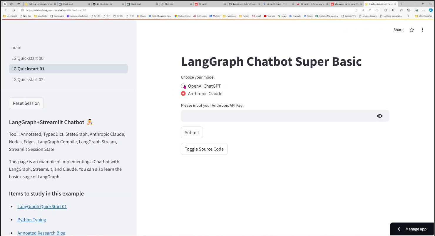
오늘 비디오는 구독자님이 Streamlit ,LangChain 그리고 LangGraph 에서 Chatbot 기능을 지원하기 위한 Memory 기능의 차이점을 문의 하셔서 거기에 대한 답변을 드리기 위해 만들었습니다.
답변을 준비하다 보니까 그냥 댓글로 몇마디 할 만한 사항이 아니더라구요.
AI 가 처음 나왔을 때 LangChain 에서는 Input Context 의 Length limit 에 대한 고민을 많이 했었던 것 같습니다.
그래서 대화 히스토리 관리하는데 있어서 input context를 줄이는 방법에 집중을 했었습니다. (Conversational Memory)
하지만 이 기능은 AI Model 들이 input context의 크기를 대폭 늘리면서 더 이상 필요성이 대두 되지는 않은 것 같습니다.
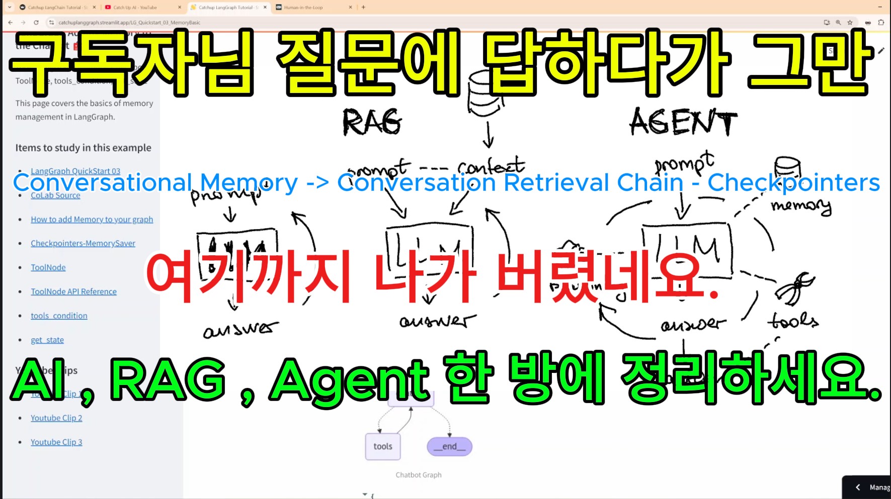
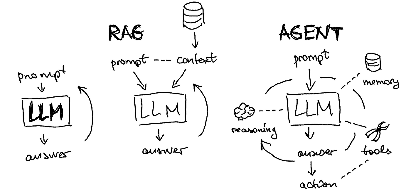
곧이어 나온 RAG 기능을 제대로 지원할 수 있는 대화 history 관리 툴을 LangChain에서는 제공 했습니다. (Conversation Retrieval Chain)
그런데 AI 세계는 멈추지 않았습니다.
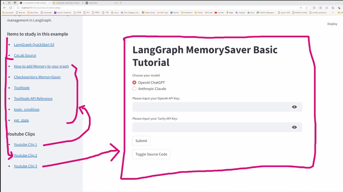
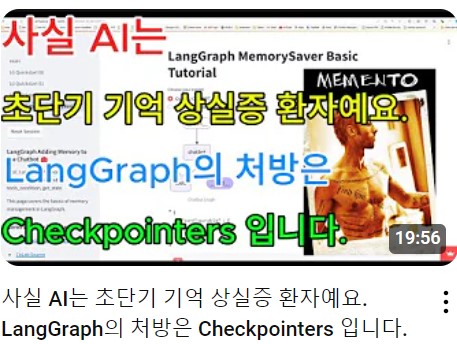
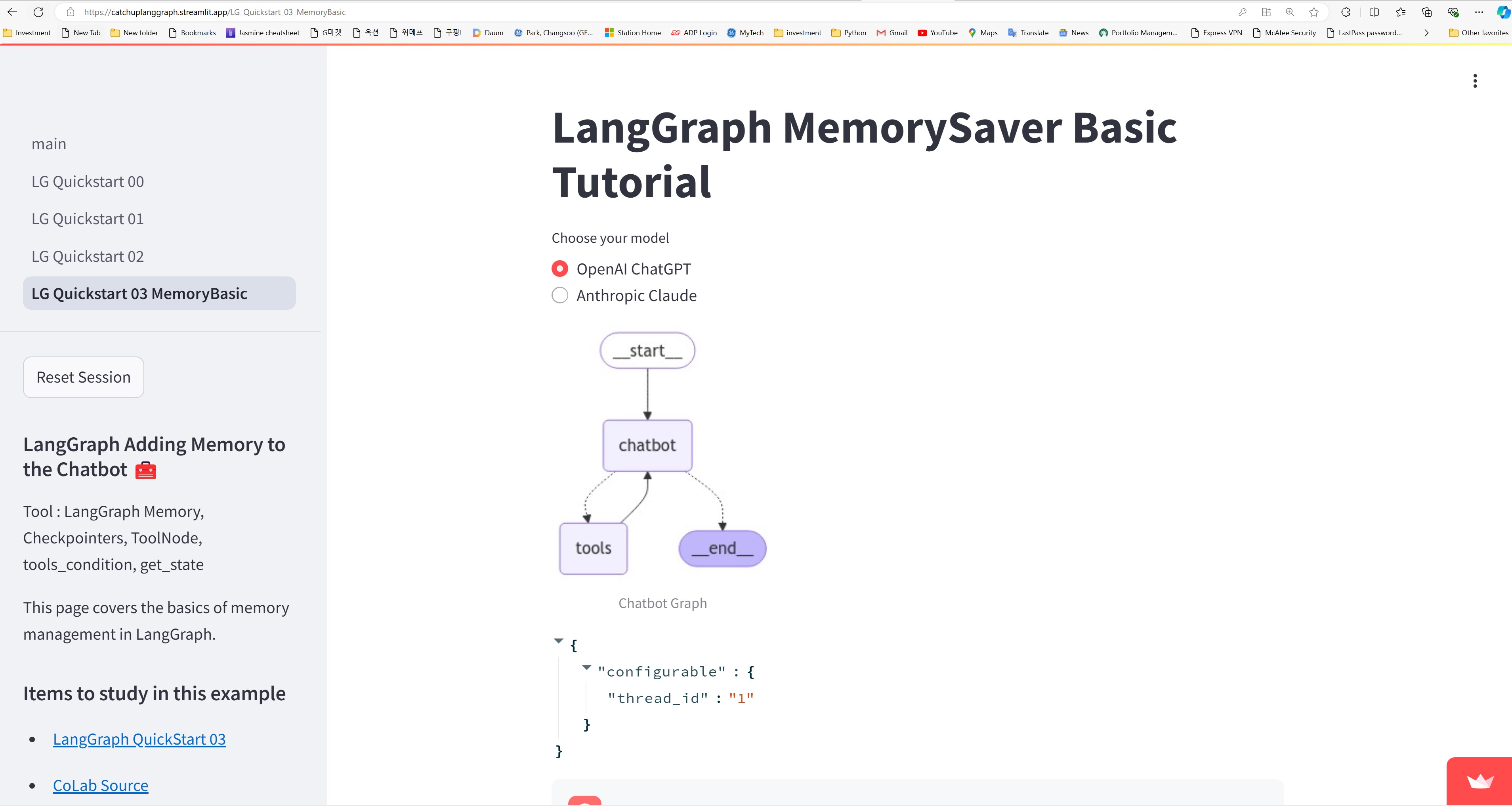
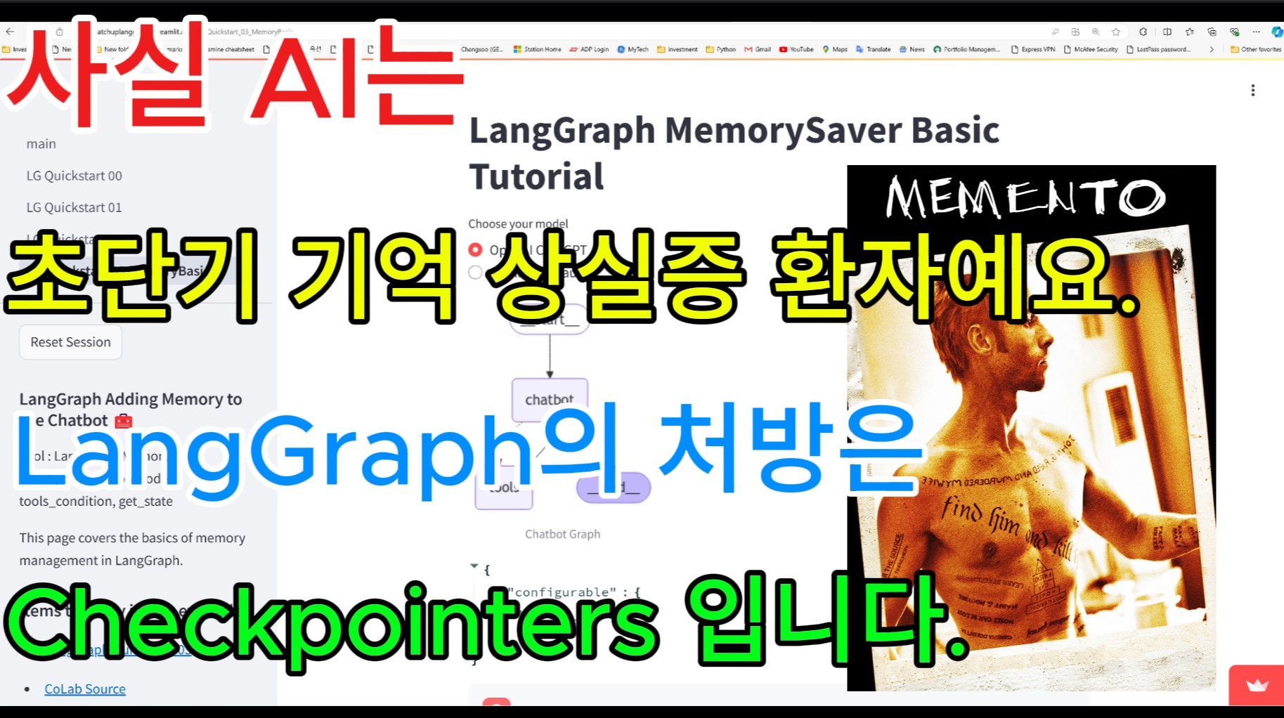
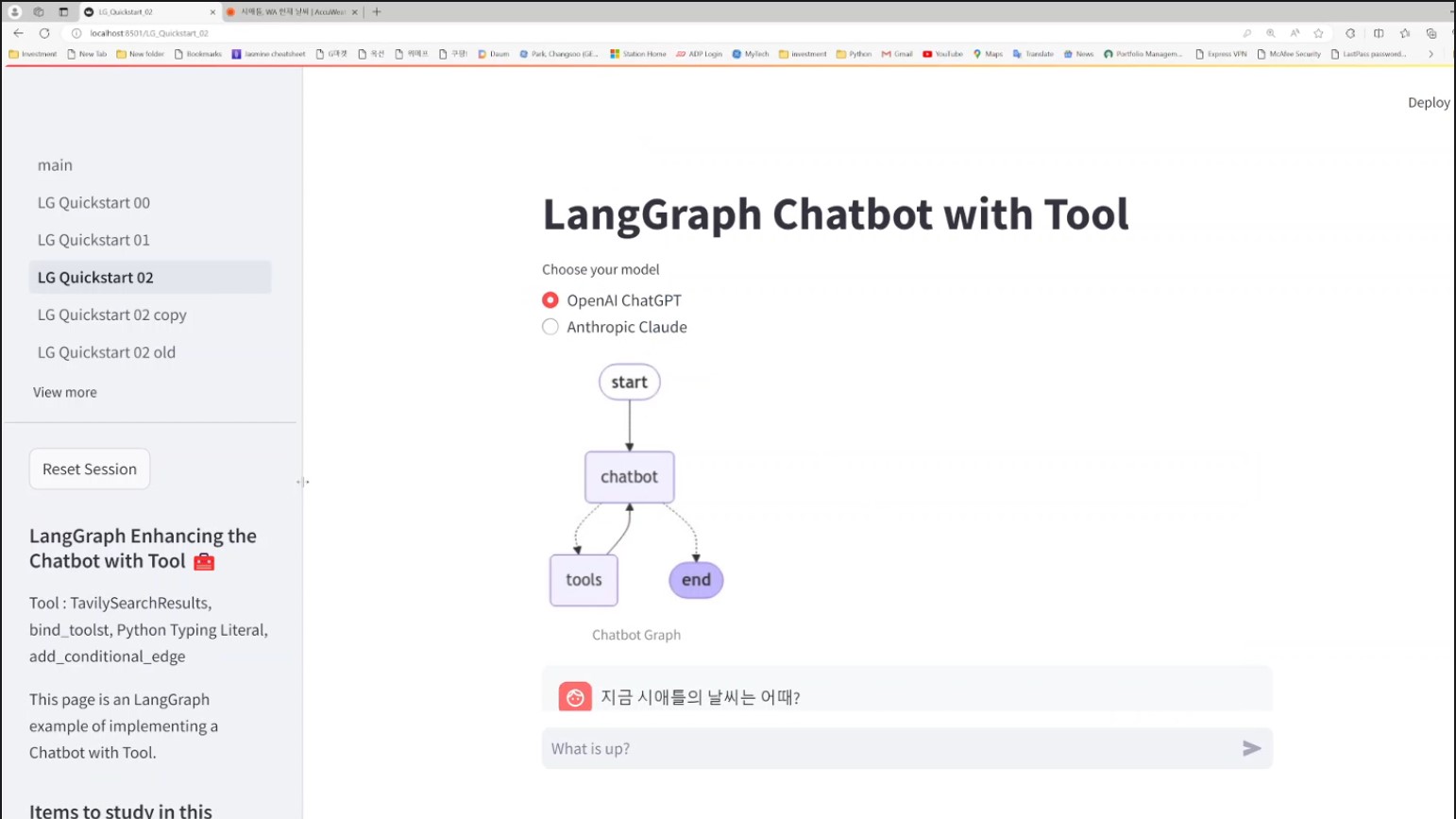
좀 더 복잡한 문제를 해결하는 AI 서비스를 제공하기 위해 AI Agent 개념이 나왔습니다. (CheckPointer)
이것을 설명하기 위해서 AI , RAG , AI Agent 이런 AI App 개발의 트렌드 변화까지 다 말하게 됐네요.
이번 기회에 한번 더 이 트랜드 변화를 정리해 보네요.
Catchup AI Portfolio · Streamlit
Catchup AI Portfolio
This app was built in Streamlit! Check it out and visit https://streamlit.io for more awesome community apps. 🎈
catchupai.streamlit.app
Catchup LangChain Tutorial · Streamlit
Catchup LangChain Tutorial
This app was built in Streamlit! Check it out and visit https://streamlit.io for more awesome community apps. 🎈
catchuplangchain.streamlit.app
Catchup LangGraph Tutorial · Streamlit
Catchup LangGraph Tutorial
This app was built in Streamlit! Check it out and visit https://streamlit.io for more awesome community apps. 🎈
catchuplanggraph.streamlit.app
반응형