

https://d2l.ai/chapter_convolutional-neural-networks/index.html
7. Convolutional Neural Networks — Dive into Deep Learning 1.0.3 documentation
d2l.ai
7.1. From Fully Connected Layers to Convolutions — Dive into Deep Learning 1.0.0-beta0 documentation
d2l.ai
7. Convolutional Neural Networks
Image data is represented as a two-dimensional grid of pixels, be the image monochromatic or in color. Accordingly each pixel corresponds to one or multiple numerical values respectively. So far we have ignored this rich structure and treated images as vectors of numbers by flattening them, irrespective of the spatial relation between pixels. This deeply unsatisfying approach was necessary in order to feed the resulting one-dimensional vectors through a fully connected MLP.
이미지 데이터는 픽셀의 2차원 격자로 표현되며, 이미지는 단색이거나 컬러입니다. 따라서 각 픽셀은 각각 하나 또는 여러 개의 숫자 값에 해당합니다. 지금까지 우리는 이 풍부한 구조를 무시하고 픽셀 간의 공간적 관계에 관계없이 이미지를 평면화하여 숫자 벡터로 처리했습니다. 완전히 연결된 MLP를 통해 결과적인 1차원 벡터를 공급하려면 매우 만족스럽지 못한 이러한 접근 방식이 필요했습니다.
Because these networks are invariant to the order of the features, we could get similar results regardless of whether we preserve an order corresponding to the spatial structure of the pixels or if we permute the columns of our design matrix before fitting the MLP’s parameters. Ideally, we would leverage our prior knowledge that nearby pixels are typically related to each other, to build efficient models for learning from image data.
이러한 네트워크는 특징의 순서에 불변하기 때문에 픽셀의 공간 구조에 해당하는 순서를 유지하는지 또는 MLP의 매개변수를 맞추기 전에 디자인 행렬의 열을 순열하는지 여부에 관계없이 비슷한 결과를 얻을 수 있습니다. 이상적으로는 근처 픽셀이 일반적으로 서로 관련되어 있다는 사전 지식을 활용하여 이미지 데이터로부터 학습하기 위한 효율적인 모델을 구축합니다.
This chapter introduces convolutional neural networks (CNNs) (LeCun et al., 1995), a powerful family of neural networks that are designed for precisely this purpose. CNN-based architectures are now ubiquitous in the field of computer vision. For instance, on the Imagnet collection (Deng et al., 2009) it was only the use of convolutional neural networks, in short Convnets, that provided significant performance improvements (Krizhevsky et al., 2012).
이 장에서는 바로 이러한 목적을 위해 설계된 강력한 신경망 계열인 CNN(Convolutional Neural Network)(LeCun et al., 1995)을 소개합니다. CNN 기반 아키텍처는 이제 컴퓨터 비전 분야 어디에서나 볼 수 있습니다. 예를 들어, Imagnet 컬렉션(Deng et al., 2009)에서는 상당한 성능 향상을 제공한 것은 컨볼루션 신경망, 줄여서 Convnets의 사용뿐이었습니다(Krizhevsky et al., 2012).
Modern CNNs, as they are called colloquially, owe their design to inspirations from biology, group theory, and a healthy dose of experimental tinkering. In addition to their sample efficiency in achieving accurate models, CNNs tend to be computationally efficient, both because they require fewer parameters than fully connected architectures and because convolutions are easy to parallelize across GPU cores (Chetlur et al., 2014). Consequently, practitioners often apply CNNs whenever possible, and increasingly they have emerged as credible competitors even on tasks with a one-dimensional sequence structure, such as audio (Abdel-Hamid et al., 2014), text (Kalchbrenner et al., 2014), and time series analysis (LeCun et al., 1995), where recurrent neural networks are conventionally used. Some clever adaptations of CNNs have also brought them to bear on graph-structured data (Kipf and Welling, 2016) and in recommender systems.
구어체로 불리는 현대 CNN은 생물학, 그룹 이론 및 건전한 실험적 조작에서 영감을 받아 설계되었습니다. 정확한 모델을 달성하기 위한 샘플 효율성 외에도 CNN은 완전히 연결된 아키텍처보다 적은 매개변수가 필요하고 컨볼루션이 GPU 코어 전체에서 병렬화되기 쉽기 때문에 계산적으로 효율적인 경향이 있습니다(Chetlur et al., 2014). 결과적으로 실무자들은 가능할 때마다 CNN을 적용하는 경우가 많으며 오디오(Abdel-Hamid et al., 2014), 텍스트(Kalchbrenner et al., 2014)와 같은 1차원 시퀀스 구조를 가진 작업에서도 점점 더 신뢰할 수 있는 경쟁자로 부상하고 있습니다. ), 시계열 분석(LeCun et al., 1995), 여기서는 순환 신경망이 일반적으로 사용됩니다. CNN의 일부 영리한 적응으로 인해 그래프 구조 데이터(Kipf and Welling, 2016)와 추천 시스템에도 적용되었습니다.
First, we will dive more deeply into the motivation for convolutional neural networks. This is followed by a walk through the basic operations that comprise the backbone of all convolutional networks. These include the convolutional layers themselves, nitty-gritty details including padding and stride, the pooling layers used to aggregate information across adjacent spatial regions, the use of multiple channels at each layer, and a careful discussion of the structure of modern architectures. We will conclude the chapter with a full working example of LeNet, the first convolutional network successfully deployed, long before the rise of modern deep learning. In the next chapter, we will dive into full implementations of some popular and comparatively recent CNN architectures whose designs represent most of the techniques commonly used by modern practitioners.
먼저, 컨볼루션 신경망의 동기에 대해 더 깊이 살펴보겠습니다. 그런 다음 모든 컨볼루션 네트워크의 백본을 구성하는 기본 작업을 살펴봅니다. 여기에는 컨벌루션 레이어 자체, 패딩 및 스트라이드를 포함한 핵심적인 세부 정보, 인접한 공간 영역에 걸쳐 정보를 집계하는 데 사용되는 풀링 레이어, 각 레이어에서 다중 채널 사용, 현대 아키텍처 구조에 대한 신중한 논의가 포함됩니다. 우리는 현대 딥러닝이 등장하기 오래 전에 성공적으로 배포된 최초의 컨볼루셔널 네트워크인 LeNet의 전체 작동 예제로 이 장을 마무리할 것입니다. 다음 장에서는 현대 실무자가 일반적으로 사용하는 대부분의 기술을 대표하는 디자인의 인기 있고 비교적 최근의 일부 CNN 아키텍처의 전체 구현에 대해 살펴보겠습니다.
7.1. From Fully Connected Layers to Conolutions
To this day, the models that we have discussed so far remain appropriate options when we are dealing with tabular data. By tabular, we mean that the data consist of rows corresponding to examples and columns corresponding to features. With tabular data, we might anticipate that the patterns we seek could involve interactions among the features, but we do not assume any structure a priori concerning how the features interact.
오늘까지 우리가 논의한 모델은 표 데이터(tabular data)를 다룰 때 적절한 옵션으로 남아 있습니다. 테이블 형식(tabular data)이란 데이터가 examples 에 해당하는 행과 features에 해당하는 열로 구성됨을 의미합니다. 테이블 형식 데이터를 사용하면 우리가 찾는 패턴이 기능(features) 간의 상호 작용을 포함할 수 있다고 예상할 수 있지만 기능(features)이 상호 작용하는 방식과 관련하여 어떤 구조도 선험적으로 가정하지 않습니다.
Deel Learning에서 Examples 와 Features 란?
In deep learning, "examples" refer to the individual data instances or observations used for training or evaluating a model. They can be images, texts, audio clips, or any other form of input data that the model processes. Examples are typically represented as tensors or arrays of numbers to be fed into the deep learning model.
딥러닝에서 "예제(Examples)"는 모델의 학습 또는 평가를 위해 사용되는 개별 데이터 인스턴스 또는 관측치를 의미합니다. 예제는 이미지, 텍스트, 오디오 클립 또는 모델이 처리하는 다른 형태의 입력 데이터일 수 있습니다. 예제는 일반적으로 텐서나 숫자 배열로 표현되어 딥러닝 모델에 공급됩니다.
"Features" in deep learning context generally refer to the input variables or attributes that are used to represent the examples. Features are derived from the raw input data and serve as the basis for making predictions or classifications. In computer vision, for example, features may include pixel values or visual descriptors extracted from images. In natural language processing, features may be word embeddings or other text representations. The choice and quality of features can significantly impact the performance and effectiveness of a deep learning model.
"특징(Features)"은 딥러닝에서 입력 변수 또는 속성을 가리키는 용어로 사용됩니다. 특징은 원시 입력 데이터로부터 파생된 값으로, 예제를 나타내는 데 사용됩니다. 특징은 예를 들어 이미지에서 픽셀 값이나 시각적 특징 기술자로 구성될 수 있습니다. 자연어 처리에서는 단어 임베딩이나 기타 텍스트 표현이 특징으로 사용될 수 있습니다. 특징의 선택과 품질은 딥러닝 모델의 성능과 효과에 중대한 영향을 미칠 수 있습니다.
Sometimes, we truly lack knowledge to guide the construction of craftier architectures. In these cases, an MLP may be the best that we can do. However, for high-dimensional perceptual data, such structure-less networks can grow unwieldy.
때때로 우리는 더 교묘한 건축물(craftier architectures)의 건설을 안내할 지식이 정말로 부족합니다. 이러한 경우 MLP가 최선일 수 있습니다. 그러나 고차원 지각 데이터의 경우 이러한 구조가 없는 네트워크는 다루기 힘들게 커질 수 있습니다.
For instance, let’s return to our running example of distinguishing cats from dogs. Say that we do a thorough job in data collection, collecting an annotated dataset of one-megapixel photographs. This means that each input to the network has one million dimensions. Even an aggressive reduction to one thousand hidden dimensions would require a fully connected layer characterized by 106×103=109 parameters. Unless we have lots of GPUs, a talent for distributed optimization, and an extraordinary amount of patience, learning the parameters of this network may turn out to be infeasible.
예를 들어, 고양이와 개를 구별하는 예제로 돌아가 봅시다. 1메가픽셀 사진의 주석이 달린 데이터 세트를 수집하는 데이터 수집 작업을 철저히 수행한다고 가정해 보겠습니다. 이것은 신경망에 대한 각 입력이 백만 개의 차원을 갖는다는 것을 의미합니다. 1000개의 은닉 차원으로 공격적으로 축소하더라도 106×103=109 매개변수로 특징지어지는 완전히 연결된 레이어가 필요합니다. 많은 GPU, 분산 최적화 능력, 엄청난 인내심이 없다면 이 네트워크의 매개변수를 학습하는 것이 불가능할 수 있습니다.
A careful reader might object to this argument on the basis that one megapixel resolution may not be necessary. However, while we might be able to get away with one hundred thousand pixels, our hidden layer of size 1000 grossly underestimates the number of hidden units that it takes to learn good representations of images, so a practical system will still require billions of parameters. Moreover, learning a classifier by fitting so many parameters might require collecting an enormous dataset. And yet today both humans and computers are able to distinguish cats from dogs quite well, seemingly contradicting these intuitions. That is because images exhibit rich structure that can be exploited by humans and machine learning models alike. Convolutional neural networks (CNNs) are one creative way that machine learning has embraced for exploiting some of the known structure in natural images.
신중한 독자라면 1메가픽셀 해상도가 필요하지 않을 수 있다는 근거로 이 주장에 반대할 수 있습니다. 그러나 10만 개의 픽셀로 벗어날 수 있지만 1000 크기의 숨겨진 레이어는 이미지의 좋은 표현을 학습하는 데 필요한 숨겨진 단위의 수를 과소 평가하므로 실제 시스템에는 여전히 수십억 개의 매개 변수가 필요합니다. 또한 너무 많은 매개변수를 피팅하여 분류기를 학습하려면 막대한 데이터 세트를 수집해야 할 수 있습니다. 그러나 오늘날 인간과 컴퓨터 모두 고양이와 개를 꽤 잘 구별할 수 있으며 이러한 직관과 모순되는 것처럼 보입니다. 이미지는 인간과 기계 학습 모델 모두가 활용할 수 있는 풍부한 구조를 보여주기 때문입니다. CNN(컨볼루션 신경망)은 기계 학습이 자연 이미지의 알려진 구조 중 일부를 활용하기 위해 채택한 창의적인 방법 중 하나입니다.
7.1.1. Invariance (불변)
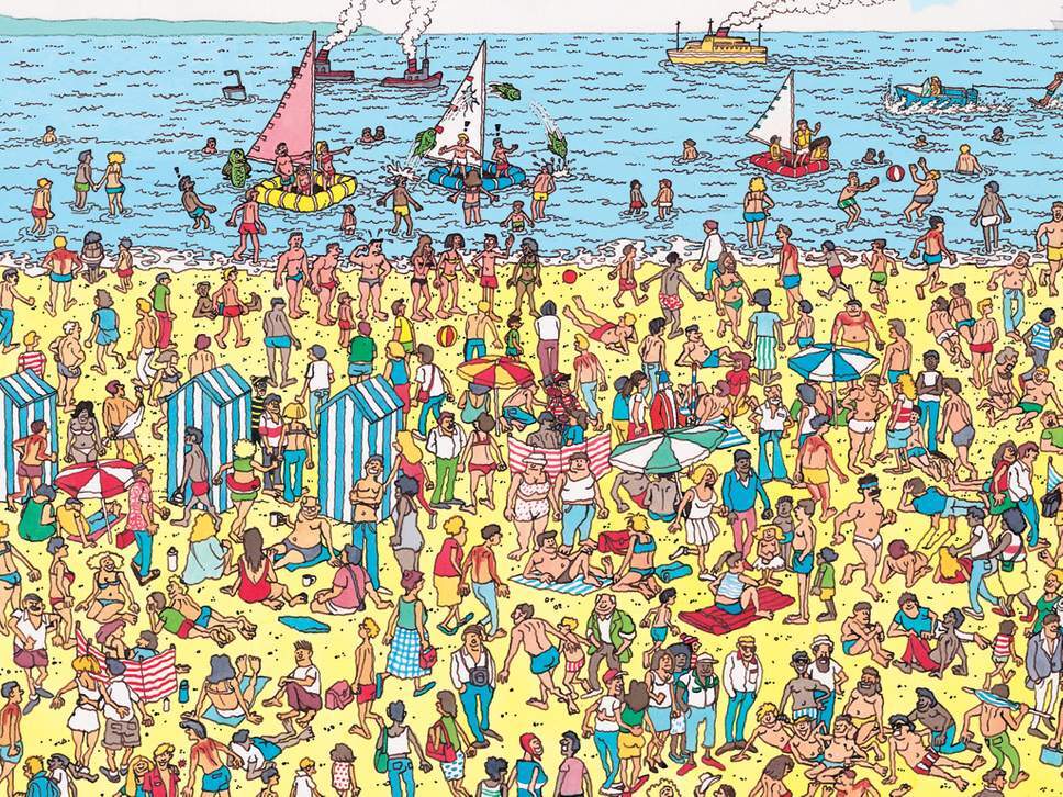
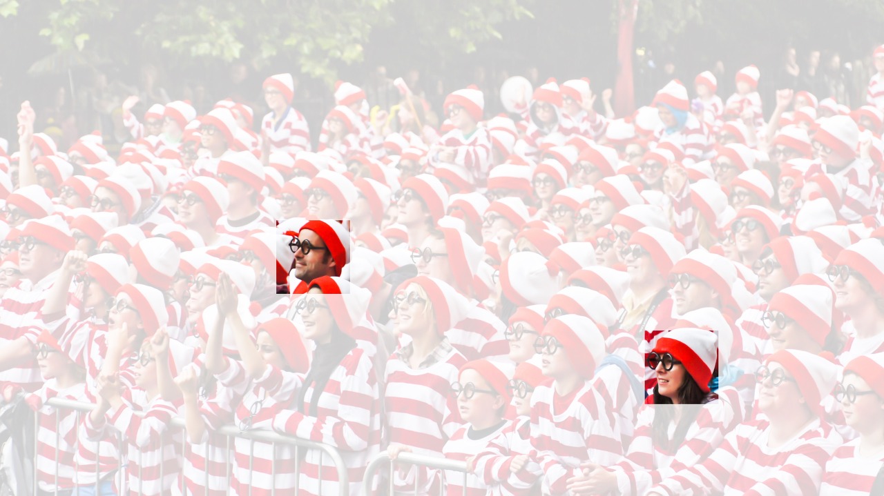
Imagine that we want to detect an object in an image. It seems reasonable that whatever method we use to recognize objects should not be overly concerned with the precise location of the object in the image. Ideally, our system should exploit this knowledge. Pigs usually do not fly and planes usually do not swim. Nonetheless, we should still recognize a pig were one to appear at the top of the image. We can draw some inspiration here from the children’s game “Where’s Waldo” (depicted in Fig. 7.1.1). The game consists of a number of chaotic scenes bursting with activities. Waldo shows up somewhere in each, typically lurking in some unlikely location. The reader’s goal is to locate him. Despite his characteristic outfit, this can be surprisingly difficult, due to the large number of distractions. However, what Waldo looks like does not depend upon where Waldo is located. We could sweep the image with a Waldo detector that could assign a score to each patch, indicating the likelihood that the patch contains Waldo. In fact, many object detection and segmentation algorithms are based on this approach (Long et al., 2015). CNNs systematize this idea of spatial invariance, exploiting it to learn useful representations with fewer parameters.
이미지를 어떤 물체인지 감지하고 싶다고 상상해 보십시오. 우리가 객체를 인식하기 위해 사용하는 방법이 무엇이든 이미지에서 객체의 정확한 위치(precise location)에 지나치게 관심을 가져서는 안 된다는 것이 합리적으로 보입니다. 이상적으로는 우리 시스템이 이 지식을 활용해야 합니다. 돼지는 일반적으로 날지 않으며 비행기는 일반적으로 수영하지 않습니다. 그럼에도 불구하고 우리는 여전히 돼지가 이미지 상단에 나타나도 돼지라는 것을 인식해야 합니다. 여기서 우리는 아이들의 게임 "Waldo는 어디에 있습니까?"(그림 7.1.1에 묘사됨)에서 약간의 영감을 얻을 수 있습니다. 이 게임은 활동으로 가득 찬 수많은 혼란스러운 장면으로 구성됩니다. Waldo는 각각 어딘가에 나타나며 일반적으로 가능성이 낮은 위치에 숨어 있습니다. 독자의 목표는 그를 찾는 것입니다. 그의 독특한 복장에도 불구하고 많은 산만함으로 인해 이것은 놀라울 정도로 어려울 수 있습니다. 그러나 Waldo의 모습은 Waldo의 위치에 따라 달라지지 않습니다. 각 패치에 점수를 할당할 수 있는 Waldo 탐지기로 이미지를 스윕하여 패치에 Waldo가 포함되어 있을 가능성을 나타낼 수 있습니다. 실제로 많은 객체 감지 및 분할 알고리즘이 이 접근 방식을 기반으로 합니다(Long et al., 2015). CNN은 이러한 공간적 불변성(spatial invariance)에 대한 아이디어를 체계화하여 이를 활용하여 더 적은 매개변수로 유용한 표현을 학습합니다.
We can now make these intuitions more concrete by enumerating a few desiderata to guide our design of a neural network architecture suitable for computer vision:
이제 우리는 컴퓨터 비전에 적합한 신경망 아키텍처 설계를 안내하기 위해 몇 가지 필요한 사항을 열거함으로써 이러한 직관을 보다 구체적으로 만들 수 있습니다.
- In the earliest layers, our network should respond similarly to the same patch, regardless of where it appears in the image. This principle is called translation invariance (or translation equivariance).
초기 레이어에서 네트워크는 이미지의 어디에 표시되는지에 관계없이 동일한 패치(patch)에 유사하게 응답해야 합니다. 이 원칙을 translation invariance (또는 translation equivariance-)이라고 합니다. - The earliest layers of the network should focus on local regions, without regard for the contents of the image in distant regions. This is the locality principle. Eventually, these local representations can be aggregated to make predictions at the whole image level.
네트워크의 가장 초기 계층은 먼 지역에 있는 이미지의 내용을 고려하지 않고 로컬 지역에 초점을 맞춰야 합니다. 이것이 지역성의 원칙(locality principle)입니다. 결국 이러한 로컬 representations 을 집계하여 전체 이미지 수준에서 예측할 수 있습니다. - As we proceed, deeper layers should be able to capture longer-range features of the image, in a way similar to higher level vision in nature.
진행함에 따라 더 깊은 레이어는 자연의 더 높은 수준의 비전과 유사한 방식으로 이미지의 장거리 기능(longer-range features)을 캡처할 수 있어야 합니다.
Let’s see how this translates into mathematics.
이것이 어떻게 수학으로 변환되는지 봅시다.
7.1.2. Constraining the MLP
To start off, we can consider an MLP with two-dimensional images X as inputs and their immediate hidden representations H similarly represented as matrices (they are two-dimensional tensors in code), where both X and H have the same shape. Let that sink in. We now conceive of not only the inputs but also the hidden representations as possessing spatial structure.
우선, 2차원 이미지 X를 입력으로 사용하는 MLP를 생각해 볼 수 있습니다. 그들의 immediate hidden representations H는 matrices(그들은 코드에서 2차원 텐서입니다.)로서 두 X와 H가 같은 모양을 갖기 때문에 유사하게 표현됩니다. 좀 더 깊이 들어 갑시다. 우리는 이제 입력뿐만 아니라 hidden representations도 spatial structure를 가지고 있다고 생각합니다.
Let [X]i,j and [H]i,j denote the pixel at location (i,j) in the input image and hidden representation, respectively. Consequently, to have each of the hidden units receive input from each of the input pixels, we would switch from using weight matrices (as we did previously in MLPs) to representing our parameters as fourth-order weight tensors W. Suppose that U contains biases, we could formally express the fully connected layer as
[X]i,j 및 [H]i,j는 각각 입력 이미지 및 hidden representation의 location (i,j)에 있는 픽셀을 나타냅니다. 결과적으로 각각의 은닉 유닛(hidden units)이 각 입력 픽셀로부터 입력을 받도록 하려면 가중치 행렬-weight matrices-(이전에 MLP에서 했던 것처럼)을 사용하는 것에서 매개변수를 4차 가중치 텐서 W(fourth-order weight tensors W)로 나타내는 것으로 전환해야 합니다. U가 편향을 포함한다고 가정합니다. 우리는 fully connected layer를 공식적으로 다음과 같이 표현할 수 있습니다.
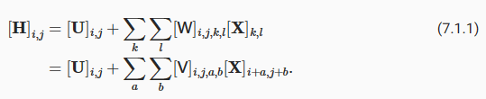
The switch from W to V is entirely cosmetic for now since there is a one-to-one correspondence between coefficients in both fourth-order tensors. We simply re-index the subscripts (k,l) such that k=i+a and l=j+b. In other words, we set [V]i,j,a,b=[W]i,j,i+a,j+b. The indices a and b run over both positive and negative offsets, covering the entire image. For any given location (i, j) in the hidden representation [H]i,j, we compute its value by summing over pixels in x, centered around (i,j) and weighted by [V]i,j,a,b. Before we carry on, let’s consider the total number of parameters required for a single layer in this parametrization: a 1000×1000 image (1 megapixel) is mapped to a 1000×1000 hidden representation. This requires 1012 parameters, far beyond what computers currently can handle.
W에서 V로의 전환은 두 4차 텐서(fourth-order tensors)의 계수(coefficients ) 사이에 일대일 대응이 있기 때문에 현재로서는 완전히 외관상(cosmetic )입니다. 우리는 단순히 k=i+a 및 l=j+b와 같이 subscripts (k,l)를 다시 인덱싱합니다. 즉, [V]i,j,a,b=[W]i,j,i+a,j+b로 설정합니다. 인덱스 a와 b는 양수 오프셋과 음수 오프셋 모두에서 실행되어 전체 이미지를 덮습니다. 숨겨진 표현(hidden representation) [H]i,j의 주어진 위치(location )(i, j)에 대해 x의 픽셀을 합산하여 값을 계산하고 (i,j)를 중심으로 [V]i,j,a,b에 의해 가중치를 적용합니다. 계속하기 전에 이 매개변수화에서 단일 레이어에 필요한 총 매개변수 수를 고려해 보겠습니다. 1000×1000 이미지(1메가픽셀)는 1000×1000 숨겨진 표현에 매핑(hidden representation)됩니다. 여기에는 컴퓨터가 현재 처리할 수 있는 것보다 훨씬 많은 1012개의 매개변수가 필요합니다.
hidden representation 이란?
Hidden representation refers to the intermediate or hidden layers of a neural network where the input data is transformed and processed before reaching the final output layer. It is a set of internal representations or features that capture relevant information about the input data.
'Hidden representation'은 신경망의 중간 또는 숨겨진 레이어로, 입력 데이터가 최종 출력 레이어에 도달하기 전에 변환되고 처리되는 부분을 의미합니다. 이는 입력 데이터에 대한 관련 정보를 포착하는 내부 표현이나 피처들의 집합입니다.
In a neural network, the hidden layers perform computations on the input data using a combination of weights, biases, and activation functions. Each hidden layer progressively extracts higher-level features or abstractions from the raw input data. These hidden representations are not directly observable or interpretable by humans but contain important information that helps the network make accurate predictions or classifications.
신경망에서는 숨겨진 레이어들이 가중치, 편향, 활성화 함수의 조합을 사용하여 입력 데이터에 대해 계산을 수행합니다. 각 숨겨진 레이어는 원시 입력 데이터로부터 점차적으로 고수준의 피처나 추상화를 추출합니다. 이러한 숨겨진 표현은 직접적으로 사람들에게 관측 가능하거나 해석 가능한 것은 아니지만, 네트워크가 정확한 예측이나 분류를 수행하는 데 도움이 되는 중요한 정보를 포함합니다.
The purpose of hidden representations is to capture meaningful and relevant patterns in the data that are useful for the specific task the neural network is designed to solve. By learning these representations through the training process, neural networks can automatically discover complex relationships and hierarchical structures in the data, leading to improved performance and generalization.
숨겨진 표현의 목적은 신경망이 해결하려는 특정 작업에 유용한 데이터의 의미 있는 패턴을 포착하는 것입니다. 훈련 과정을 통해 이러한 표현을 학습함으로써 신경망은 데이터에서 복잡한 관계와 계층 구조를 자동으로 발견할 수 있습니다. 이를 통해 성능과 일반화 능력이 향상됩니다.
Overall, hidden representations play a crucial role in deep learning as they enable the network to learn and represent data in a more compact and expressive form, facilitating effective information processing and learning.
전반적으로, 숨겨진 표현은 딥 러닝에서 중요한 역할을 하며, 네트워크가 데이터를 더 간결하고 표현력이 풍부한 형태로 학습하고 표현할 수 있도록 돕습니다. 이는 효과적인 정보 처리와 학습을 가능하게 하며, 네트워크의 성능 향상에 기여합니다.
7.1.2.1. Translation Invariance
Now let’s invoke the first principle established above: translation invariance (Zhang and others, 1988). This implies that a shift in the input X should simply lead to a shift in the hidden representation H. This is only possible if V and U do not actually depend on (i,j). As such, we have [V]i,j,a,b=[V]a,b and U is a constant, say u. As a result, we can simplify the definition for H:
이제 위에서 확립한 첫 번째 원칙인 변환 불변성(translation invariance)을 적용해 보겠습니다(Zhang and others, 1988). 이는 입력 X의 이동이 단순히 숨겨진 표현(hidden representation) H의 이동으로 이어져야 함을 의미합니다. 이것은 V와 U가 실제로 (i,j)에 의존하지 않는 경우에만 가능합니다. 따라서 [V]i,j,a,b=[V]a,b이고 U는 상수입니다. 결과적으로 H에 대한 정의를 단순화할 수 있습니다.
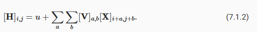
This is a convolution! We are effectively weighting pixels at (i+a,j+b) in the vicinity of location (i,j) with coefficients [V]a,b to obtain the value [H]i,j. Note that [V]a,b needs many fewer coefficients than [V]i,j,a,b since it no longer depends on the location within the image. Consequently, the number of parameters required is no longer 1012 but a much more reasonable 4⋅106: we still have the dependency on a,b∈(−1000,1000). In short, we have made significant progress. Time-delay neural networks (TDNNs) are some of the first examples to exploit this idea (Waibel et al., 1989).
이것은 convolution입니다! 값 [H]i,j를 얻기 위해 계수(coefficients)a,b를 사용하여 위치 (i,j) 부근의 (i+a,j+b)에 있는 픽셀에 효과적으로 가중치를 부여합니다. [V]a,b는 더 이상 이미지 내의 위치에 의존하지 않기 때문에 [V]i,j,a,b보다 훨씬 적은 계수가 필요합니다. 결과적으로 필요한 매개변수의 수는 더 이상 1012가 아니라 훨씬 더 합리적인 4⋅106입니다. 여전히 a,b∈(−1000,1000)에 대한 종속성이 있습니다. 요컨대, 우리는 상당한 진전을 이루었습니다. 시간 지연 신경망-Time-delay neural networks-(TDNN)은 이 아이디어를 활용한 첫 번째 사례 중 일부입니다(Waibel et al., 1989).
Translation Invariance란?
Translation invariance in convolutional neural networks (CNNs) refers to the property of CNNs to recognize patterns or features in an input image regardless of their position or location within the image. It means that if an object or feature is present in different parts of the image, the CNN will be able to detect and identify it regardless of its specific location.
합성곱 신경망(Convolutional Neural Networks, CNNs)의 변환 불변성(Translation Invariance)은 CNN이 입력 이미지 내에서 위치나 위치에 관계없이 패턴이나 특징을 인식하는 성질을 의미합니다. 이는 이미지 내에 객체나 특징이 다른 위치에 존재할 경우, CNN이 그것을 인식하고 식별할 수 있다는 것을 의미합니다.
CNNs achieve translation invariance through the use of convolutional layers and pooling layers. Convolutional layers apply filters or kernels to scan the entire input image, detecting local patterns or features. These filters are shared across the entire image, allowing the CNN to learn and recognize the same patterns regardless of their position. Pooling layers further enhance translation invariance by downsampling the feature maps, reducing the spatial dimensions while retaining important features.
CNN은 합성곱 계층(Convolutional Layers)과 풀링 계층(Pooling Layers)을 사용하여 변환 불변성을 달성합니다. 합성곱 계층은 필터 또는 커널을 사용하여 전체 입력 이미지를 스캔하며 지역적인 패턴이나 특징을 감지합니다. 이러한 필터는 이미지 전체에 걸쳐 공유되며, CNN은 위치에 상관없이 동일한 패턴을 학습하고 인식할 수 있습니다. 풀링 계층은 특징 맵을 다운샘플링하여 공간적인 차원을 줄이고 중요한 특징을 유지함으로써 변환 불변성을 강화합니다.
This translation invariance property makes CNNs well-suited for tasks such as image classification, object detection, and image segmentation, where the position or location of objects or features within an image may vary. It enables CNNs to effectively learn and generalize spatial patterns across different parts of an image.
이러한 변환 불변성은 CNN을 이미지 분류, 객체 탐지, 이미지 세그멘테이션과 같은 작업에 적합하게 만듭니다. 이미지 내 객체나 특징의 위치가 다양하게 변할 수 있는 경우에도 CNN은 효과적으로 공간 패턴을 학습하고 일반화할 수 있게 됩니다.
7.1.2.2. Locality
Now let’s invoke the second principle: locality. As motivated above, we believe that we should not have to look very far away from location (i,j) in order to glean relevant information to assess what is going on at [H]i,j. This means that outside some range |a|>Δ or |b|>Δ, we should set [V]a,b=0. Equivalently, we can rewrite [H]i,j as
이제 두 번째 원칙인 지역성을 적용해 보겠습니다. 위에서 동기부여된 바와 같이, 우리는 [H]i,j에서 무슨 일이 일어나고 있는지 평가하기 위해 관련 정보를 수집하기 위해 위치 (i,j)에서 아주 멀리 볼 필요가 없다고 믿습니다. 이는 어떤 범위 |a|>Δ 또는 |b|>Δ를 벗어나면 [V]a,b=0으로 설정해야 함을 의미합니다. 마찬가지로 [H]i,j를 다음과 같이 다시 쓸 수 있습니다.
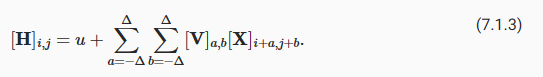
This reduces the number of parameters from 4⋅106 to 4Δ2, where Δ is typically smaller than 10. As such, we reduced the number of parameters by another 4 orders of magnitude. Note that (7.1.3), in a nutshell, is what is called a convolutional layer. Convolutional neural networks (CNNs) are a special family of neural networks that contain convolutional layers. In the deep learning research community, V is referred to as a convolution kernel, a filter, or simply the layer’s weights that are learnable parameters.
이렇게 하면 매개변수 수가 4⋅106에서 4Δ2로 줄어듭니다. 여기서 Δ는 일반적으로 10보다 작습니다. 따라서 매개변수 수를 4배 더 줄였습니다. 간단히 말해서 (7.1.3)은 컨볼루션 레이어(convolutional layer)라고 합니다. 컨볼루션 신경망-Convolutional neural networks-(CNN)은 컨볼루션 레이어(convolutional layer)를 포함하는 neural networks의 special family입니다. 딥 러닝 연구 커뮤니티에서 V는 컨볼루션 커널(convolution kernel), 필터 또는 단순히 학습 가능한 매개변수인 레이어의 가중치(weights )라고 합니다.
While previously, we might have required billions of parameters to represent just a single layer in an image-processing network, we now typically need just a few hundred, without altering the dimensionality of either the inputs or the hidden representations. The price paid for this drastic reduction in parameters is that our features are now translation invariant and that our layer can only incorporate local information, when determining the value of each hidden activation. All learning depends on imposing inductive bias. When that bias agrees with reality, we get sample-efficient models that generalize well to unseen data. But of course, if those biases do not agree with reality, e.g., if images turned out not to be translation invariant, our models might struggle even to fit our training data.
이전에는 이미지 처리 네트워크의 단일 레이어를 나타내기 위해 수십억 개의 매개변수가 필요했지만 이제는 입력 또는 숨겨진 표현(hidden representations)의 차원을 변경하지 않고 일반적으로 수백 개만 필요합니다. 이러한 매개 변수의 급격한 감소에 대해 지불한 대가는 우리의 기능이 이제 변환 불변(translation invariant)이고 레이어가 각 숨겨진 활성화 값을 결정할 때 로컬 정보만 통합할 수 있다는 것입니다. 모든 학습은 귀납적 편향(inductive bias)을 부과하는 데 달려 있습니다. 그 편견(bias )이 현실과 일치할 때 우리는 보이지 않는 데이터에 잘 일반화되는 sample-efficient models을 얻습니다. 그러나 물론 이러한 편향(bias )이 현실과 일치하지 않는 경우(예: 이미지가 변환 불변(translation invariant)이 아닌 것으로 판명된 경우) 모델이 훈련 데이터에 맞추는 데 어려움을 겪을 수 있습니다.
This dramatic reduction in parameters brings us to our last desideratum, namely that deeper layers should represent larger and more complex aspects of an image. This can be achieved by interleaving nonlinearities and convolutional layers repeatedly.
이러한 매개변수의 극적인 감소는 마지막 요구사항, 즉 더 깊은 레이어가 이미지의 더 크고 더 복잡한 측면을 나타내야 한다는 점을 의미합니다. 이는 비선형성과 컨벌루션 레이어를 반복적으로 interleaving 하여 달성할 수 있습니다.
7.1.3. Convolutions
Let’s briefly review why (7.1.3) is called a convolution. In mathematics, the convolution between two functions (Rudin, 1973), say f,g:ℝd→ℝ is defined as
(7.1.3)이 컨볼루션이라고 불리는 이유를 간단히 살펴보겠습니다. 수학에서 f,g:ℝd→ℝ와 같이 두 함수 간의 컨볼루션(Rudin, 1973)은 다음과 같이 정의됩니다.
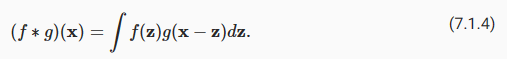
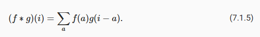
That is, we measure the overlap between f and g when one function is “flipped” and shifted byx. Whenever we have discrete objects, the integral turns into a sum. For instance, for vectors from the set of square summable infinite dimensional vectors with index running over ℤ we obtain the following definition:
즉, 하나의 함수가 "플립"되고 x만큼 이동될 때 f와 g 사이의 중첩을 측정합니다. 이산 객체(discrete objects)가 있을 때마다 적분(integral)은 합계로 바뀝니다. 예를 들어, 인덱스가 ℤ 이상인 제곱 합산 가능한 무한 차원 벡터 세트의 벡터에 대해 다음 정의를 얻습니다.
For two-dimensional tensors, we have a corresponding sum with indices (a,b) for f and (i−a,j−b) for g, respectively:
2차원 텐서의 경우 각각 f에 대한 인덱스 (a,b)와 g에 대한 (i-a,j-b)의 해당 합계가 있습니다.

This looks similar to (7.1.3), with one major difference. Rather than using (i+a,j+b), we are using the difference instead. Note, though, that this distinction is mostly cosmetic since we can always match the notation between (7.1.3) and (7.1.6). Our original definition in (7.1.3) more properly describes a cross-correlation. We will come back to this in the following section.
이것은 (7.1.3)과 비슷해 보이지만 한 가지 중요한 차이점이 있습니다. (i+a,j+b)를 사용하는 대신 차이점을 대신 사용합니다. 하지만 (7.1.3)과 (7.1.6) 사이의 표기법을 항상 일치시킬 수 있기 때문에 이 구별은 대부분 외형적(cosmetic )입니다. (7.1.3)의 원래 정의는 교차 상관(cross-correlation)을 더 적절하게 설명합니다. 이에 대해서는 다음 섹션에서 다시 설명하겠습니다.
7.1.4. Channels
Returning to our Waldo detector, let’s see what this looks like. The convolutional layer picks windows of a given size and weighs intensities according to the filter V, as demonstrated in Fig. 7.1.2. We might aim to learn a model so that wherever the “waldoness” is highest, we should find a peak in the hidden layer representations.
Waldo 감지기로 돌아가서 이것이 어떻게 보이는지 봅시다. 컨볼루션 레이어는 주어진 크기의 창을 선택하고 그림 7.1.2에서 보여지는 것처럼 필터 V에 따라 강도를 가중합니다. "waldoness"가 가장 높은 곳에서 숨겨진 레이어 표현에서 최고점을 찾도록 모델 학습을 목표로 할 수 있습니다.
There is just one problem with this approach. So far, we blissfully ignored that images consist of 3 channels: red, green, and blue. In sum, images are not two-dimensional objects but rather third-order tensors, characterized by a height, width, and channel, e.g., with shape 1024×1024×3 pixels. While the first two of these axes concern spatial relationships, the third can be regarded as assigning a multidimensional representation to each pixel location. We thus index X as [X]i,j,k. The convolutional filter has to adapt accordingly. Instead of [V]a,b, we now have [V]a,b,c.
이 접근 방식에는 한 가지 문제가 있습니다. 지금까지 우리는 이미지가 빨강, 초록, 파랑의 3개 채널로 구성되어 있다는 사실을 다행스럽게도 무시했습니다. 요컨대 이미지는 2차원 객체가 아니라 높이, 너비 및 채널(예: 1024×1024×3 픽셀 모양)로 특징지어지는 3차 텐서입니다. 이러한 축 중 처음 두 개는 공간 관계(spatial relationships)와 관련이 있지만 세 번째 축은 각 픽셀 위치에 다차원 표현을 할당하는 것으로 간주할 수 있습니다. 따라서 X를 [X]i,j,k로 인덱싱합니다. 컨벌루션 필터는 그에 따라 adapt 해야 합니다. [V]a,b 대신 이제 [V]a,b,c가 있습니다.
Moreover, just as our input consists of a third-order tensor, it turns out to be a good idea to similarly formulate our hidden representations as third-order tensors H. In other words, rather than just having a single hidden representation corresponding to each spatial location, we want an entire vector of hidden representations corresponding to each spatial location. We could think of the hidden representations as comprising a number of two-dimensional grids stacked on top of each other. As in the inputs, these are sometimes called channels. They are also sometimes called feature maps, as each provides a spatialized set of learned features to the subsequent layer. Intuitively, you might imagine that at lower layers that are closer to inputs, some channels could become specialized to recognize edges while others could recognize textures.
또한 입력이 3차 텐서로 구성되는 것처럼 숨겨진 표현을 3차 텐서 H로 유사하게 공식화하는 것이 좋습니다. 즉, 각 공간 위치에 해당하는 단일 숨겨진 표현(hidden representation)이 아니라 각 공간 위치에 해당하는 숨겨진 표현(hidden representation)의 전체 벡터가 필요합니다. 숨겨진 표현(hidden representation)은 서로 위에 쌓인 여러 개의 2차원 그리드로 구성되어 있다고 생각할 수 있습니다. 입력과 마찬가지로 이를 채널이라고도 합니다. 각각은 학습된 기능의 공간화된 세트를 후속 계층에 제공하기 때문에 기능 맵이라고도 합니다. 직관적으로 입력에 더 가까운 하위 레이어에서 일부 채널은 가장자리를 인식하도록 특수화되고 다른 채널은 텍스처를 인식할 수 있다고 상상할 수 있습니다.
To support multiple channels in both inputs (X) and hidden representations (H), we can add a fourth coordinate to V: [V]a,b,c,d. Putting everything together we have:
입력(X)과 숨겨진 표현(H) 모두에서 다중 채널을 지원하기 위해 V에 네 번째 좌표인 [V]a,b,c,d를 추가할 수 있습니다. 모든 것을 종합하면 다음과 같습니다.
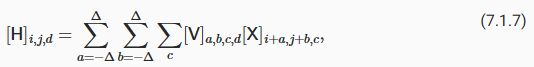
where d indexes the output channels in the hidden representations H. The subsequent convolutional layer will go on to take a third-order tensor, H, as input. Being more general, (7.1.7) is the definition of a convolutional layer for multiple channels, where V is a kernel or filter of the layer.
여기서 d는 숨겨진 표현 H의 출력 채널을 인덱싱합니다. 후속 컨볼루션 레이어는 계속해서 3차 텐서 H를 입력으로 사용합니다. 보다 일반적으로 (7.1.7)은 다중 채널에 대한 컨볼루션 계층의 정의이며, 여기서 V는 계층의 커널 또는 필터입니다.
There are still many operations that we need to address. For instance, we need to figure out how to combine all the hidden representations to a single output, e.g., whether there is a Waldo anywhere in the image. We also need to decide how to compute things efficiently, how to combine multiple layers, appropriate activation functions, and how to make reasonable design choices to yield networks that are effective in practice. We turn to these issues in the remainder of the chapter.
해결해야 할 작업이 여전히 많이 있습니다. 예를 들어, 모든 숨겨진 표현을 단일 출력으로 결합하는 방법을 알아내야 합니다(예: 이미지 어디에나 Waldo가 있는지 여부). 또한 효율적으로 계산하는 방법, 여러 계층을 결합하는 방법, 적절한 활성화 기능, 실제로 효과적인 네트워크를 생성하기 위해 합리적인 설계 선택을 하는 방법을 결정해야 합니다. 이 장의 나머지 부분에서 이러한 문제를 살펴보겠습니다.
7.1.5. Summary and Discussion
In this section we derived the structure of convolutional neural networks from first principles. While it is unclear whether this is what led to the invention of CNNs, it is satisfying to know that they are the right choice when applying reasonable principles to how image processing and computer vision algorithms should operate, at least at lower levels. In particular, translation invariance in images implies that all patches of an image will be treated in the same manner. Locality means that only a small neighborhood of pixels will be used to compute the corresponding hidden representations. Some of the earliest references to CNNs are in the form of the Neocognitron (Fukushima, 1982).
이 섹션에서는 첫 번째 원칙에서 컨볼루션 신경망의 구조를 도출했습니다. 이것이 CNN의 발명으로 이어졌는지 여부는 불분명하지만 이미지 처리 및 컴퓨터 비전 알고리즘이 적어도 낮은 수준에서 작동하는 방식에 합리적인 원칙을 적용할 때 CNN이 올바른 선택이라는 것을 알게 되어 만족스럽습니다. 특히 이미지의 변환 불변성은 이미지의 모든 패치가 동일한 방식으로 처리됨을 의미합니다. 지역성은 해당 숨겨진 표현을 계산하는 데 작은 픽셀 이웃만 사용됨을 의미합니다. CNN에 대한 초기 참조 중 일부는 Neocognitron의 형태입니다(Fukushima, 1982).
A second principle that we encountered in our reasoning is how to reduce the number of parameters in a function class without limiting its expressive power, at least, whenever certain assumptions on the model hold. We saw a dramatic reduction of complexity as a result of this restriction, turning computationally and statistically infeasible problems into tractable models.
추론에서 만난 두 번째 원칙은 적어도 모델에 대한 특정 가정이 유지될 때마다 표현력을 제한하지 않고 함수 클래스의 매개변수 수를 줄이는 방법입니다. 우리는 이 제한의 결과로 복잡성이 극적으로 감소하여 계산 및 통계적으로 실행 불가능한 문제를 다루기 쉬운 모델로 바꾸는 것을 보았습니다.
Adding channels allowed us to bring back some of the complexity that was lost due to the restrictions imposed on the convolutional kernel by locality and translation invariance. Note that channels are quite a natural addition beyond red, green, and blue. Many satellite images, in particular for agriculture and meteorology, have tens to hundreds of channels, generating hyperspectral images instead. They report data on many different wavelengths. In the following we will see how to use convolutions effectively to manipulate the dimensionality of the images they operate on, how to move from location-based to channel-based representations and how to deal with large numbers of categories efficiently.
채널을 추가하면 지역성 및 번역 불변성에 의해 컨볼루션 커널에 부과된 제한으로 인해 손실된 복잡성을 일부 되돌릴 수 있었습니다. 채널은 빨강, 녹색 및 파랑 이외의 자연스러운 추가 사항입니다. 특히 농업 및 기상학을 위한 많은 위성 이미지에는 수십에서 수백 개의 채널이 있으며 대신 하이퍼스펙트럼 이미지를 생성합니다. 그들은 다양한 파장에 대한 데이터를 보고합니다. 다음에서는 콘볼루션을 효과적으로 사용하여 작동하는 이미지의 차원을 조작하는 방법, 위치 기반 표현에서 채널 기반 표현으로 이동하는 방법 및 많은 수의 범주를 효율적으로 처리하는 방법을 살펴봅니다.
7.1.6. Exercises
'Dive into Deep Learning > D2L Convolutional Neural Networks (CNN)' 카테고리의 다른 글
| D2L - 8.3. Network in Network (NiN) (0) | 2023.07.11 |
|---|---|
| D2L - 8.2. Networks Using Blocks (VGG) (0) | 2023.07.10 |
| D2L - 8.1. Deep Convolutional Neural Networks (AlexNet) (0) | 2023.07.10 |
| D2L - 8. Modern Convolutional Neural Networks (0) | 2023.07.10 |
| D2L - 7.6. Convolutional Neural Networks (LeNet) (0) | 2023.07.09 |
| D2L - 7.5. Pooling (1) | 2023.07.09 |
| D2L - 7.4. Multiple Input and Multiple Output Channels (0) | 2023.07.09 |
| D2L - 7.3. Padding and Stride (0) | 2023.07.09 |
| D2L - 7.2. Convolutions for Images (0) | 2023.07.09 |
| D2L - 7. Convolutional Neural Networks (0) | 2023.07.09 |