

7.2. Convolutions for Images — Dive into Deep Learning 1.0.0-beta0 documentation (d2l.ai)
7.2. Convolutions for Images — Dive into Deep Learning 1.0.0-beta0 documentation
d2l.ai
7.2. Convolutions for Images
Now that we understand how convolutional layers work in theory, we are ready to see how they work in practice. Building on our motivation of convolutional neural networks as efficient architectures for exploring structure in image data, we stick with images as our running example.
이제 컨볼루션 레이어가 이론적으로 어떻게 작동하는지 이해했으므로 실제로 어떻게 작동하는지 확인할 준비가 되었습니다. 이미지 데이터의 구조를 탐색하기 위한 효율적인 아키텍처로서의 convolutional neural networks에 대한 motivation을 Building on 하겠습니다. 우리는 이미지들을 실행 예제로 사용할 것입니다.
import torch
from torch import nn
from d2l import torch as d2l
7.2.1. The Cross-Correlation Operation
Recall that strictly speaking, convolutional layers are a misnomer, since the operations they express are more accurately described as cross-correlations. Based on our descriptions of convolutional layers in Section 7.1, in such a layer, an input tensor and a kernel tensor are combined to produce an output tensor through a cross-correlation operation.
엄밀히 말하면 컨볼루션 레이어(convolutional layers)는 잘못된 이름이라는 것을 상기하세요. 왜냐하면 그들이 표현하는 연산은 cross-correlations라고 말하는 것이 더 정확한 표현이기 때문입니다. 7.1절의 컨벌루션 레이어에 대한 설명을 기반으로 이러한 레이어에서 입력 텐서와 커널 텐서를 결합하여 cross-correlation 연산을 통해 출력 텐서를 생성합니다.
cross-correlation operation이란?
Cross-correlation is a mathematical operation that measures the similarity between two signals or sequences as they are shifted relative to each other. In the context of image processing and convolutional neural networks (CNNs), cross-correlation is commonly used for feature detection and matching.
교차 상관(Cross-correlation)은 두 신호 또는 시퀀스가 서로 이동하면서 유사성을 측정하는 수학적 연산입니다. 이미지 처리와 합성곱 신경망(CNN)의 맥락에서는 교차 상관이 특징 감지와 매칭에 일반적으로 사용됩니다.
In cross-correlation, the two signals are multiplied together at each position of the shift and then summed up. This process provides a measure of similarity or correlation between the two signals. When applied to image processing, it involves sliding a filter or kernel over an input image and computing the similarity between the filter and the corresponding image region.
교차 상관에서 두 신호는 서로의 이동 위치에서 곱해진 후 합산됩니다. 이 과정은 두 신호 간의 유사성이나 상관성을 측정하는 척도를 제공합니다. 이미지 처리에 적용할 때는 필터나 커널을 입력 이미지 위에 슬라이딩시켜 필터와 해당 이미지 영역 사이의 유사성을 계산합니다.
Cross-correlation is useful in tasks such as image recognition, object detection, and pattern matching. By comparing the similarity between a given feature or pattern and different regions of an image, cross-correlation allows for the identification of relevant features or objects.
교차 상관은 이미지 인식, 물체 감지, 패턴 매칭 등과 같은 작업에서 유용합니다. 주어진 특징이나 패턴과 이미지의 다양한 영역 간의 유사성을 비교함으로써 교차 상관은 관련 특징이나 객체를 식별하는 데 사용됩니다.
Let’s ignore channels for now and see how this works with two-dimensional data and hidden representations. In Fig. 7.2.1, the input is a two-dimensional tensor with a height of 3 and width of 3. We mark the shape of the tensor as 3×3 or (3, 3). The height and width of the kernel are both 2. The shape of the kernel window (or convolution window) is given by the height and width of the kernel (here it is 2×2).
지금은 채널을 무시하고 이것이 2차원 데이터 및 숨겨진 표현(hidden representations)에서 어떻게 작동하는지 살펴보겠습니다. 그림 7.2.1에서 입력은 높이가 3이고 너비가 3인 2차원 텐서입니다. 텐서의 모양을 3×3 또는 (3, 3)으로 표시합니다. 커널의 높이와 너비는 모두 2입니다. 커널 창(또는 컨볼루션 창)의 모양은 커널의 높이와 너비로 지정됩니다(여기서는 2×2).
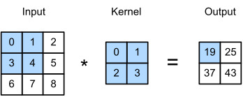
In the two-dimensional cross-correlation operation, we begin with the convolution window positioned at the upper-left corner of the input tensor and slide it across the input tensor, both from left to right and top to bottom. When the convolution window slides to a certain position, the input subtensor contained in that window and the kernel tensor are multiplied elementwise and the resulting tensor is summed up yielding a single scalar value. This result gives the value of the output tensor at the corresponding location. Here, the output tensor has a height of 2 and width of 2 and the four elements are derived from the two-dimensional cross-correlation operation:
2차원 교차 상관 연산에서는 입력 텐서의 왼쪽 위 모서리에 있는 컨볼루션 창에서 시작하여 왼쪽에서 오른쪽으로 그리고 위에서 아래로 입력 텐서를 가로질러 슬라이드합니다. 컨볼루션 윈도우가 특정 위치로 슬라이드되면 해당 윈도우에 포함된 입력 하위 텐서와 커널 텐서가 요소별로 곱해지고 결과 텐서가 합산되어 단일 스칼라 값이 생성됩니다. 이 결과는 해당 위치에서 출력 텐서의 값을 제공합니다. 여기서 출력 텐서는 높이가 2이고 너비가 2이며 4개의 요소는 2차원 교차 상관 연산에서 파생됩니다.
Note that along each axis, the output size is slightly smaller than the input size. Because the kernel has width and height greater than one, we can only properly compute the cross-correlation for locations where the kernel fits wholly within the image, the output size is given by the input size nℎ×bw minus the size of the convolution kernel kℎ×kw via
각 축을 따라 출력 크기는 입력 크기보다 약간 작습니다. 커널의은 1보다 큰 너비와 높이가 있기 때문에 우리는 location에 대한 cross-correlation 계산만 할 수 있습니다. 출력 크기는 다음을 거쳐서 입력 크기 nℎ×nw에서 컨볼루션 커널 크기 kℎ×kw를 뺀 값입니다.

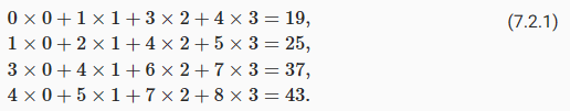
This is the case since we need enough space to “shift” the convolution kernel across the image. Later we will see how to keep the size unchanged by padding the image with zeros around its boundary so that there is enough space to shift the kernel. Next, we implement this process in the corr2d function, which accepts an input tensor X and a kernel tensor K and returns an output tensor Y.
이것은 이미지에서 컨볼루션 커널을 "shift"할 충분한 공간이 필요하기 때문입니다. 나중에 커널을 이동할 충분한 공간이 있도록 이미지 경계 주위에 0을 채워 크기를 변경하지 않고 유지하는 방법을 살펴보겠습니다. 다음으로 입력 텐서 X와 커널 텐서 K를 받아들이고 출력 텐서 Y를 반환하는 corr2d 함수에서 이 프로세스를 구현합니다.
def corr2d(X, K):  #@save
    """Compute 2D cross-correlation."""
    h, w = K.shape
    Y = torch.zeros((X.shape[0] - h + 1, X.shape[1] - w + 1))
    for i in range(Y.shape[0]):
        for j in range(Y.shape[1]):
            Y[i, j] = (X[i:i + h, j:j + w] * K).sum()
    return Y
위 코드는 2D 크로스-상관(correlation) 연산을 수행하는 함수인 corr2d를 구현한 코드입니다.
해당 코드를 한 줄씩 설명하면 다음과 같습니다:
- def corr2d(X, K): : corr2d라는 함수를 정의하고, X와 K라는 두 개의 인자를 받습니다. X는 입력 데이터이고, K는 커널(필터)입니다.
- h, w = K.shape : 커널의 높이 h와 너비 w를 추출합니다.
- Y = torch.zeros((X.shape[0] - h + 1, X.shape[1] - w + 1)) : 출력을 저장할 Y 텐서를 생성합니다. Y의 크기는 입력 데이터와 커널의 크기에 따라 결정됩니다.
- for i in range(Y.shape[0]): : Y의 행을 반복합니다.
- for j in range(Y.shape[1]): : Y의 열을 반복합니다.
- Y[i, j] = (X[i:i + h, j:j + w] * K).sum() : 입력 데이터 X와 커널 K 사이의 2D 크로스-상관 값을 계산하여 Y에 저장합니다. 이를 위해 입력 데이터와 커널을 요소별로 곱한 후 합을 구합니다.
- return Y : 계산된 출력 텐서 Y를 반환합니다.
이 함수는 입력 데이터 X와 커널 K 사이의 2D 크로스-상관 값을 계산하여 출력하는 함수입니다. 크로스-상관은 입력 데이터와 커널 간의 유사성을 측정하는데 사용되며, 주로 이미지 처리에서 필터와 이미지의 관련성을 파악하는 데 활용됩니다.
We can construct the input tensor X and the kernel tensor K from Fig. 7.2.1 to validate the output of the above implementation of the two-dimensional cross-correlation operation.
그림 7.2.1에서 입력 텐서 X와 커널 텐서 K를 구성하여 위의 2차원 교차 상관 연산의 출력을 검증할 수 있습니다.
X = torch.tensor([[0.0, 1.0, 2.0], [3.0, 4.0, 5.0], [6.0, 7.0, 8.0]])
K = torch.tensor([[0.0, 1.0], [2.0, 3.0]])
corr2d(X, K)
위 코드는 주어진 입력 데이터 X와 커널 K를 이용하여 corr2d 함수를 호출하는 코드입니다.
해당 코드를 한 줄씩 설명하면 다음과 같습니다:
- X = torch.tensor([[0.0, 1.0, 2.0], [3.0, 4.0, 5.0], [6.0, 7.0, 8.0]]) : 입력 데이터인 X를 정의합니다. 이는 크기가 3x3인 텐서로, 2D 매트릭스 형태의 데이터입니다.
- K = torch.tensor([[0.0, 1.0], [2.0, 3.0]]) : 커널인 K를 정의합니다. 이는 크기가 2x2인 텐서로, 2D 매트릭스 형태의 필터입니다.
- corr2d(X, K) : corr2d 함수를 호출하여 입력 데이터 X와 커널 K 사이의 2D 크로스-상관 값을 계산합니다.
즉, 주어진 입력 데이터 X와 커널 K를 사용하여 corr2d 함수를 호출하고, 2D 크로스-상관 값을 계산하는 결과를 반환합니다. 이를 통해 입력 데이터와 커널 사이의 유사성을 측정하고, 컨볼루션 연산을 수행할 수 있습니다.
7.2.2. Convolutional Layers
A convolutional layer cross-correlates the input and kernel and adds a scalar bias to produce an output. The two parameters of a convolutional layer are the kernel and the scalar bias. When training models based on convolutional layers, we typically initialize the kernels randomly, just as we would with a fully connected layer.
컨볼루션 계층은 입력과 커널(혹은 필터)을 상호 연관(cross-correlates)시키고 스칼라 편향(scalar bias)을 추가하여 출력을 생성합니다. 컨볼루션 레이어의 두 매개변수는 커널과 스칼라 편향((scalar bias))입니다. 컨벌루션 레이어를 기반으로 모델을 교육할 때 일반적으로 완전히 연결된 레이어에서와 마찬가지로 커널을 무작위로 초기화합니다.
scalar bias란?
In the context of a convolutional layer, the scalar bias refers to a single constant value that is added to each output channel of the convolutional operation. It is an additional learnable parameter in the convolutional layer, apart from the kernel/filter weights.
합성곱 층에서의 스칼라 편향은 커널(필터)과 별개로 각 출력 채널에 더해지는 단일 상수값을 의미합니다. 합성곱 층에서 스칼라 편향은 커널 가중치 외에 추가적인 학습 가능한 매개변수입니다.
During the convolution operation, the input data is convolved with the kernel weights, and the resulting values are summed along with the scalar bias for each output channel. The scalar bias helps introduce an additional degree of freedom in the model by allowing the network to shift the output values based on the bias term.
합성곱 연산 과정에서 입력 데이터는 커널 가중치와 합성곱되고, 각 출력 채널에 대해 스칼라 편향이 더해집니다. 스칼라 편향은 신경망에게 추가적인 자유도를 부여하여 편향 항에 따라 출력 값을 조정할 수 있게 합니다.
The scalar bias allows the network to adjust the baseline or offset of the output feature maps, enabling the model to capture and represent more complex patterns and relationships in the data. It provides flexibility in modeling data with varying levels of intensity or activation.
스칼라 편향은 출력 특징 맵의 기준선 또는 오프셋을 조정할 수 있도록 합니다. 이를 통해 모델은 데이터의 다양한 강도나 활성화 수준에 따라 출력 값을 조절할 수 있게 됩니다.
In summary, the scalar bias is a single constant value added to the output channels of a convolutional layer to introduce an offset or baseline to the feature maps. It helps the model capture and represent complex patterns and relationships in the data.
요약하면, 스칼라 편향은 합성곱 층의 출력 채널에 더해지는 단일 상수값으로, 특징 맵에 기준선 또는 오프셋을 도입합니다. 이를 통해 모델은 데이터의 복잡한 패턴과 관계를 포착하고 표현할 수 있습니다.
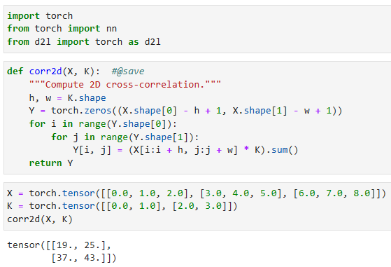
We are now ready to implement a two-dimensional convolutional layer based on the corr2d function defined above. In the __init__ constructor method, we declare weight and bias as the two model parameters. The forward propagation method calls the corr2d function and adds the bias.
이제 위에서 정의한 corr2d 함수를 기반으로 2차원 컨볼루션 계층을 구현할 준비가 되었습니다. __init__ 생성자 메서드에서 가중치와 편향을 두 모델 매개변수로 선언합니다. 정방향 전파 방법은 corr2d 함수를 호출하고 바이어스를 추가합니다.
class Conv2D(nn.Module):
    def __init__(self, kernel_size):
        super().__init__()
        self.weight = nn.Parameter(torch.rand(kernel_size))
        self.bias = nn.Parameter(torch.zeros(1))

    def forward(self, x):
return corr2d(x, self.weight) + self.bias- Conv2D 클래스는 nn.Module을 상속하는 합성곱 층을 정의합니다.
- __init__ 메서드는 합성곱 커널 크기(kernel_size)를 입력으로 받고, 초기화 작업을 수행합니다.
- self.weight는 커널 가중치를 나타내는 파라미터로 정의됩니다. torch.rand(kernel_size)를 사용하여 랜덤한 초기값으로 초기화됩니다.
- self.bias는 스칼라 편향을 나타내는 파라미터로 정의됩니다. 초기값으로 0을 가집니다.
- forward 메서드는 입력(x)을 받고, corr2d 함수를 사용하여 입력과 커널 가중치의 합성곱을 계산합니다. 그리고 스칼라 편향(self.bias)을 더한 결과를 반환합니다.
이 코드는 합성곱 층을 정의하고, 커널 가중치와 스칼라 편향을 포함한 학습 가능한 매개변수를 가지고 있습니다. 입력과 커널의 합성곱 결과에 편향을 더한 값이 출력으로 반환됩니다.
In ℎ×w convolution or a ℎ×w convolution kernel, the height and width of the convolution kernel are ℎ and w, respectively. We also refer to a convolutional layer with a ℎ×w convolution kernel simply as a ℎ×w convolutional layer.
ℎ×w 컨볼루션 또는 ℎ×w 컨볼루션 커널에서 컨볼루션 커널의 높이와 너비는 각각 ℎ와 w입니다. 또한 ℎ×w 컨볼루션 커널이 있는 컨볼루션 레이어를 단순히 ℎ×w 컨볼루션 레이어라고 합니다.
7.2.3. Object Edge Detection in Images
Let’s take a moment to parse a simple application of a convolutional layer: detecting the edge of an object in an image by finding the location of the pixel change. First, we construct an “image” of 6×8 pixels. The middle four columns are black (0) and the rest are white (1).
컨볼루션 레이어의 간단한 애플리케이션을 파싱하는 시간을 가져보겠습니다. 픽셀 변화의 위치를 찾아 이미지에서 객체의 가장자리를 감지합니다. 먼저 6×8 픽셀의 "이미지"를 구성합니다. 가운데 4개 열은 검은색(0)이고 나머지는 흰색(1)입니다.
X = torch.ones((6, 8))
X[:, 2:6] = 0
X- X는 크기가 (6, 8)인 텐서로 초기값은 모두 1로 설정됩니다.
- X[:, 2:6] = 0은 X 텐서의 모든 행(:)에서 열 인덱스 2부터 6 전까지의 범위에 해당하는 요소들을 0으로 변경합니다. 즉, 2부터 5까지의 열에 해당하는 값들을 0으로 설정합니다.
- X를 출력하면 변경된 텐서가 나타납니다.
이 코드는 크기가 (6, 8)인 텐서 X를 생성한 후, 열 인덱스 2부터 5까지의 범위에 해당하는 요소들을 0으로 변경합니다. 변경된 X 텐서가 출력됩니다.
Next, we construct a kernel K with a height of 1 and a width of 2. When we perform the cross-correlation operation with the input, if the horizontally adjacent elements are the same, the output is 0. Otherwise, the output is non-zero. Note that this kernel is special case of a finite difference operator. At location (i,j) it computes xi,j−x(i+1),j', i.e., it computes the difference between the values of horizontally adjacent pixels. This is a discrete approximation of the first derivative in the horizontal direction. After all, for a function f(i,j) its derivative −∂if(i,j)=limϵ→0 f(i,j)−f(i+ϵ,j)/ϵ. Let’s see how this works in practice.
다음으로 높이가 1이고 너비가 2인 커널 K를 구성합니다. 입력으로 교차 상관 연산을 수행할 때 가로로 인접한 요소가 같으면 출력은 0입니다. 그렇지 않으면 출력은 0이 아닙니다. 이 커널은 유한 차분 연산자(finite difference operator)의 특수한 경우입니다. 위치 (i,j)에서 xi,j−x(i+1),j'를 계산합니다. 즉, 수평으로 인접한 픽셀 값 간의 차이를 계산합니다. 이것은 수평 방향에서 1차 도함수의 이산 근사치(discrete approximation)입니다. 결국, 함수 f(i,j)의 경우 파생물 −∂if(i,j)=limϵ→0 f(i,j)−f(i+ϵ,j)/ϵ입니다. 이것이 실제로 어떻게 작동하는지 봅시다.
K = torch.tensor([[1.0, -1.0]])- K는 크기가 (1, 2)인 텐서로 초기값은 [1.0, -1.0]으로 설정됩니다.
이 코드는 크기가 (1, 2)인 텐서 K를 생성하고, 초기값으로 [1.0, -1.0]을 사용합니다.
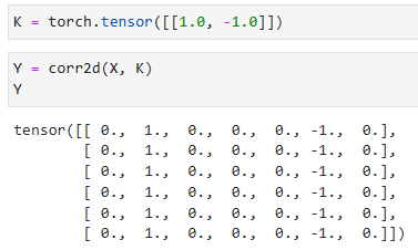
We are ready to perform the cross-correlation operation with arguments X (our input) and K (our kernel). As you can see, we detect 1 for the edge from white to black and -1 for the edge from black to white. All other outputs take value 0.
인수 X(입력) 및 K(커널)를 사용하여 cross-correlation 연산을 수행할 준비가 되었습니다. 보시다시피 흰색에서 검은색으로의 가장자리에 대해 1을 감지하고 검은색에서 흰색으로의 가장자리에 대해 -1을 감지합니다. 다른 모든 출력은 값이 0입니다.
Y = corr2d(X, K)
Y- Y는 corr2d 함수에 X와 K를 입력으로 전달하여 얻은 결과입니다.
이 코드는 X와 K를 corr2d 함수에 입력으로 전달하여 얻은 결과를 Y에 할당합니다. Y는 corr2d 함수의 결과값입니다.
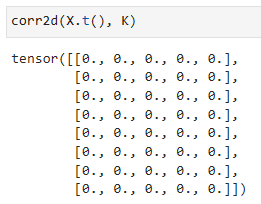
We can now apply the kernel to the transposed image. As expected, it vanishes. The kernel K only detects vertical edges.
이제 커널을 전치된 이미지(transposed image)에 적용할 수 있습니다. 예상대로 사라집니다. 커널 K는 수직 에지만 감지합니다.
corr2d(X.t(), K)- corr2d 함수에 X.t()와 K를 입력으로 전달하여 호출합니다.
- X.t()는 X의 전치(transpose)를 반환하는 연산입니다. 이는 X의 행과 열을 바꾼 행렬을 의미합니다.
- 따라서 corr2d 함수는 X의 전치된 행렬과 K를 입력으로 받아 결과를 계산합니다.
7.2.4. Learning a Kernel
Designing an edge detector by finite differences [1, -1] is neat if we know this is precisely what we are looking for. However, as we look at larger kernels, and consider successive layers of convolutions, it might be impossible to specify precisely what each filter should be doing manually.
유한 차이(finite differences) [1, -1]로 edge detector를 설계하는 것은 이것이 우리가 찾고 있는 것이 정확히 무엇인지 안다면 깔끔합니다. 그러나 더 큰 커널을 살펴보고 연속적인 컨볼루션 레이어를 고려할 때 각 필터가 수동으로 수행해야 하는 작업을 정확하게 지정하는 것이 불가능할 수 있습니다.
Now let’s see whether we can learn the kernel that generated Y from X by looking at the input–output pairs only. We first construct a convolutional layer and initialize its kernel as a random tensor. Next, in each iteration, we will use the squared error to compare Y with the output of the convolutional layer. We can then calculate the gradient to update the kernel. For the sake of simplicity, in the following we use the built-in class for two-dimensional convolutional layers and ignore the bias.
이제 입력-출력 쌍만 보고 X에서 Y를 생성한 커널을 학습할 수 있는지 살펴보겠습니다. 먼저 컨볼루션 레이어를 구성하고 커널을 랜덤 텐서로 초기화합니다. 다음으로 각 반복에서 제곱 오차를 사용하여 Y를 컨볼루션 레이어의 출력과 비교합니다. 그런 다음 기울기를 계산하여 커널을 업데이트할 수 있습니다. 단순화를 위해 다음에서는 2차원 컨볼루션 레이어에 내장 클래스를 사용하고 바이어스를 무시합니다.
# Construct a two-dimensional convolutional layer with 1 output channel and a
# kernel of shape (1, 2). For the sake of simplicity, we ignore the bias here
conv2d = nn.LazyConv2d(1, kernel_size=(1, 2), bias=False)

# The two-dimensional convolutional layer uses four-dimensional input and
# output in the format of (example, channel, height, width), where the batch
# size (number of examples in the batch) and the number of channels are both 1
X = X.reshape((1, 1, 6, 8))
Y = Y.reshape((1, 1, 6, 7))
lr = 3e-2  # Learning rate

for i in range(10):
    Y_hat = conv2d(X)
    l = (Y_hat - Y) ** 2
    conv2d.zero_grad()
    l.sum().backward()
    # Update the kernel
    conv2d.weight.data[:] -= lr * conv2d.weight.grad
    if (i + 1) % 2 == 0:
        print(f'epoch {i + 1}, loss {l.sum():.3f}')
첫째줄은 (conv2d = nn.LazyConv2d(1, kernel_size=(1, 2), bias=False))
- 1개의 출력 채널과 (1, 2) 크기의 커널을 가지는 2D 컨볼루션 레이어(conv2d)를 생성합니다.
- 여기서는 편향(bias)을 고려하지 않고 설정합니다.
- X와 Y를 4차원 형태로 변형하여 입력합니다. 입력과 출력은 (예제 개수, 채널 수, 높이, 너비) 형식을 따릅니다.
- 여기서는 배치 크기(배치에 있는 예제 수)와 채널 수가 모두 1인 형태로 설정합니다.
- lr은 학습률(learning rate)로, 0.03으로 설정합니다.
for loop 문은
- 10번의 에폭(epoch) 동안 학습을 수행합니다.
- conv2d(X)를 통해 예측값 Y_hat을 계산합니다.
- 손실 함수 l은 예측값과 실제값의 차이의 제곱으로 정의됩니다.
- conv2d.zero_grad()를 통해 기울기를 초기화합니다.
- l.sum().backward()를 통해 손실을 역전파합니다.
- 커널을 업데이트합니다. 업데이트는 학습률과 기울기를 이용하여 수행됩니다.
- 매 2번째 에폭마다 손실을 출력합니다.
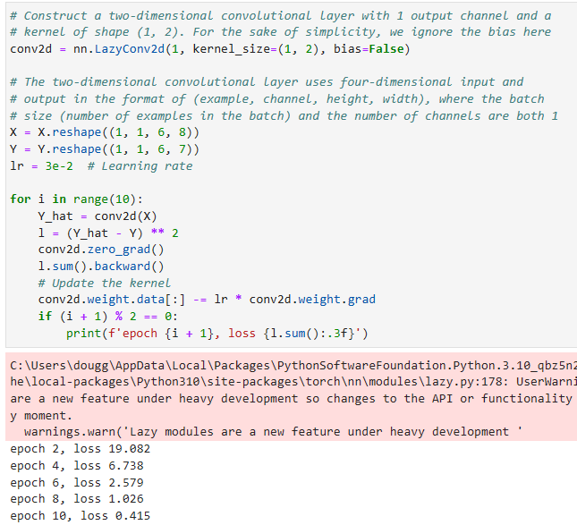
Note that the error has dropped to a small value after 10 iterations. Now we will take a look at the kernel tensor we learned.
오류는 10회 반복 후 작은 값으로 떨어졌습니다. 이제 우리가 배운 커널 텐서를 살펴보겠습니다.
conv2d.weight.data.reshape((1, 2))- conv2d의 가중치(weight)를 (1, 2) 크기로 변형합니다.
- 가중치는 2D 컨볼루션 레이어에 사용되는 커널(kernel)을 나타냅니다.
- (1, 2) 크기로 변형된 가중치는 1개의 출력 채널과 2개의 요소를 가지는 형태로 재구성됩니다.
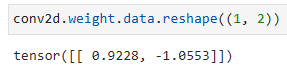
Indeed, the learned kernel tensor is remarkably close to the kernel tensor K we defined earlier.
실제로 학습된 커널 텐서는 이전에 정의한 커널 텐서 K에 매우 가깝습니다.
7.2.5. Cross-Correlation and Convolution
Recall our observation from Section 7.1 of the correspondence between the cross-correlation and convolution operations. Here let’s continue to consider two-dimensional convolutional layers. What if such layers perform strict convolution operations as defined in (7.1.6) instead of cross-correlations? In order to obtain the output of the strict convolution operation, we only need to flip the two-dimensional kernel tensor both horizontally and vertically, and then perform the cross-correlation operation with the input tensor.
교차 상관과 컨볼루션 연산 사이의 대응에 대한 섹션 7.1의 관찰을 상기하십시오. 여기서 계속해서 2차원 컨볼루션 레이어를 살펴보겠습니다. 이러한 레이어가 교차 상관 대신 (7.1.6)에 정의된 엄격한 컨벌루션 연산을 수행한다면 어떻게 될까요? 엄격한 컨벌루션 연산의 출력을 얻기 위해서는 2차원 커널 텐서를 수평 및 수직으로 뒤집은 다음 입력 텐서와 교차 상관 연산을 수행하면 됩니다.
It is noteworthy that since kernels are learned from data in deep learning, the outputs of convolutional layers remain unaffected no matter such layers perform either the strict convolution operations or the cross-correlation operations.
커널은 딥 러닝의 데이터에서 학습되기 때문에 컨볼루션 레이어의 출력은 이러한 레이어가 strict convolution operations또는 cross-correlation operations을 수행하는 것과 상관없이 영향을 받지 않습니다.
To illustrate this, suppose that a convolutional layer performs cross-correlation and learns the kernel in Fig. 7.2.1, which is denoted as the matrix K here. Assuming that other conditions remain unchanged, when this layer performs strict convolution instead, the learned kernel K′ will be the same as K after K′ is flipped both horizontally and vertically. That is to say, when the convolutional layer performs strict convolution for the input in Fig. 7.2.1 and K′, the same output in Fig. 7.2.1 (cross-correlation of the input and K) will be obtained.
이를 설명하기 위해 합성곱 계층이 교차 상관을 수행하고 여기에서 행렬 K로 표시되는 그림 7.2.1의 커널을 학습한다고 가정합니다. 다른 조건이 변하지 않는다고 가정하면, 이 레이어가 대신 엄격한 컨볼루션을 수행하면 학습된 커널 K'는 K'가 수평 및 수직으로 뒤집힌 후 K와 동일할 것입니다. 즉, convolutional layer가 그림 7.2.1의 입력과 K'에 대해 엄격한 컨벌루션을 수행하면 그림 7.2.1과 동일한 출력(입력과 K의 상호 상관)이 얻어집니다.
In keeping with standard terminology with deep learning literature, we will continue to refer to the cross-correlation operation as a convolution even though, strictly-speaking, it is slightly different. Besides, we use the term element to refer to an entry (or component) of any tensor representing a layer representation or a convolution kernel.
딥 러닝 문헌의 표준 용어에 따라 엄밀히 말하면 약간 다르지만 cross-correlation operation 을 convolution 으로 계속 언급할 것입니다. 게다가 element 라는 용어는 layer representation 또는 convolution kernel을 나타내는 모든 텐서의 entry (또는 component)을 참조하는 데 사용됩니다.
7.2.6. Feature Map and Receptive Field
As described in Section 7.1.4, the convolutional layer output in Fig. 7.2.1 is sometimes called a feature map, as it can be regarded as the learned representations (features) in the spatial dimensions (e.g., width and height) to the subsequent layer. In CNNs, for any element x of some layer, its receptive field refers to all the elements (from all the previous layers) that may affect the calculation of x during the forward propagation. Note that the receptive field may be larger than the actual size of the input.
섹션 7.1.4에서 설명한 것처럼 그림 7.2.1의 컨볼루션 레이어 출력은 spatial dimensions(예: 너비 및 높이)에서 subsequent layer로 가면서 learned representations (features)으로 간주될 수 있으므로 feature map이라고도 합니다. CNN에서 일부 계층의 모든 요소 x에 대해 수용 필드는 순방향 전파 중에 x 계산에 영향을 미칠 수 있는 모든 이전 계층의 요소를 참조합니다. 수용 필드는 입력의 실제 크기보다 클 수 있습니다.
Let’s continue to use Fig. 7.2.1 to explain the receptive field. Given the 2×2 convolution kernel, the receptive field of the shaded output element (of value 19) is the four elements in the shaded portion of the input. Now let’s denote the 2×2 output as Y and consider a deeper CNN with an additional 2×2 convolutional layer that takes Y as its input, outputting a single element z. In this case, the receptive field of z on Y includes all the four elements of Y, while the receptive field on the input includes all the nine input elements. Thus, when any element in a feature map needs a larger receptive field to detect input features over a broader area, we can build a deeper network.
계속해서 그림 7.2.1을 사용하여 수용 필드를 설명하겠습니다. 2×2 컨볼루션 커널이 주어지면 음영 처리된 출력 요소(값 19)의 수용 필드는 입력의 음영 처리된 부분에 있는 4개의 요소입니다. 이제 2×2 출력을 Y로 표시하고 Y를 입력으로 사용하여 단일 요소 z를 출력하는 추가 2×2 컨벌루션 레이어가 있는 더 깊은 CNN을 고려해 보겠습니다. 이 경우 Y에 대한 z의 수용 필드는 Y의 네 가지 요소를 모두 포함하고 입력의 수용 필드는 9개의 입력 요소를 모두 포함합니다. 따라서 기능 맵의 요소가 더 넓은 영역에서 입력 기능을 감지하기 위해 더 큰 수용 필드가 필요한 경우 더 깊은 네트워크를 구축할 수 있습니다.
Receptive fields derive their name from neurophysiology. In a series of experiments (Hubel and Wiesel, 1959, Hubel and Wiesel, 1962, Hubel and Wiesel, 1968) on a range of animals and different stimuli, Hubel and Wiesel explored the response of what is called the visual cortex on said stimuli. By and large they found that lower levels respond to edges and related shapes. Later on, Field (1987) illustrated this effect on natural images with, what can only be called, convolutional kernels. We reprint a key figure in Fig. 7.2.2 to illustrate the striking similarities.
수용 분야는 신경생리학에서 이름을 따왔습니다. 다양한 동물과 다양한 자극에 대한 일련의 실험(Hubel과 Wiesel, 1959, Hubel과 Wiesel, 1962, Hubel과 Wiesel, 1968)에서 Hubel과 Wiesel은 상기 자극에 대한 시각 피질이라고 불리는 것의 반응을 탐구했습니다. 전반적으로 그들은 낮은 수준이 가장자리 및 관련 모양에 반응한다는 것을 발견했습니다. 나중에 Field(1987)는 컨볼루션 커널이라고만 할 수 있는 자연 이미지에 대한 이 효과를 설명했습니다. 놀라운 유사성을 설명하기 위해 그림 7.2.2의 핵심 수치를 다시 인쇄합니다.
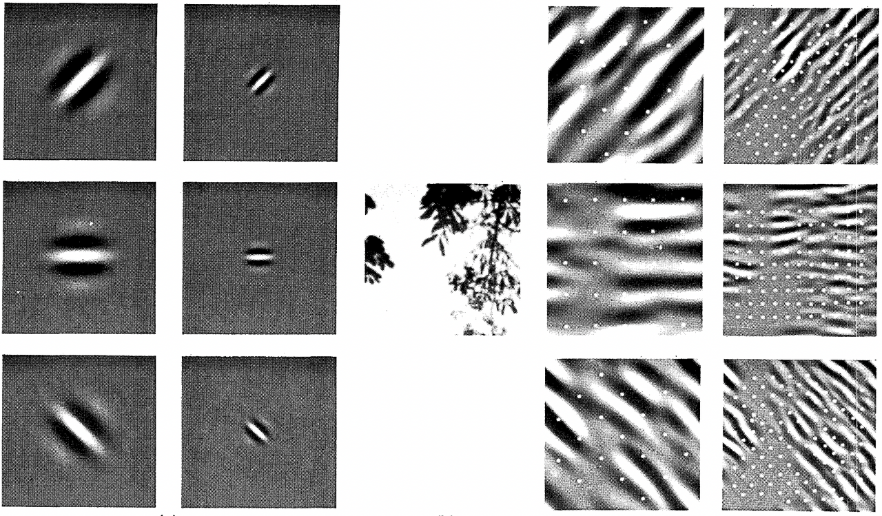
As it turns out, this relation even holds for the features computed by deeper layers of networks trained on image classification tasks, as demonstrated e.g., in Kuzovkin et al. (2018). Suffice it to say, convolutions have proven to be an incredibly powerful tool for computer vision, both in biology and in code. As such, it is not surprising (in hindsight) that they heralded the recent success in deep learning.
결과적으로 Kuzovkin et al. (2018)에서 보여 주었듯 이 관계는 이미지 분류 작업에 대해 훈련된 더 깊은 네트워크 계층에서 계산된 기능에도 적용됩니다. 컨볼루션은 생물학과 코드 모두에서 컴퓨터 비전을 위한 매우 강력한 도구임이 입증되었습니다. 따라서 그들이 최근 딥 러닝의 성공을 예고한 것은 (돌이켜보면) 놀라운 일이 아닙니다.
7.2.7. Summary
The core computation required for a convolutional layer is a cross-correlation operation. We saw that a simple nested for-loop is all that is required to compute its value. If we have multiple input and multiple output channels, we are performing a matrix-matrix operation between channels. As can be seen, the computation is straightforward and, most importantly, highly local. This affords significant hardware optimization and many recent results in computer vision are only possible due to that. After all, it means that chip designers can invest into fast computation rather than memory, when it comes to optimizing for convolutions. While this may not lead to optimal designs for other applications, it opens the door to ubiquitous and affordable computer vision.
컨볼루션 계층에 필요한 핵심 계산은 cross-correlation operation입니다. 값을 계산하는 데 필요한 것은 간단한 중첩 for-loop 뿐입니다. 입력 채널과 출력 채널이 여러 개인 경우 채널 간에 행렬-행렬 연산(matrix-matrix operation)을 수행합니다. 여러분이 보았듯이 계산은 직관적이고 가장 중요한 것은 highly local 이라는 점입니다. 이것은 상당한 하드웨어 최적화를 제공하며 컴퓨터 비전의 많은 최근 결과는 그로 인해 가능합니다. 결국 이는 칩 설계자가 컨볼루션을 최적화할 때 메모리가 아닌 빠른 계산에 투자할 수 있음을 의미합니다. 이것은 다른 응용 프로그램에 대한 최적의 설계로 이어지지 않을 수 있지만 유비쿼터스 및 저렴한 컴퓨터 비전의 문을 엽니다.
In terms of convolutions themselves, they can be used for many purposes such as to detect edges and lines, to blur images, or to sharpen them. Most importantly, it is not necessary that the statistician (or engineer) invents suitable filters. Instead, we can simply learn them from data. This replaces feature engineering heuristics by evidence-based statistics. Lastly, and quite delightfully, these filters are not just advantageous for building deep networks but they also correspond to receptive fields and feature maps in the brain. This gives us confidence that we are on the right track.
컨볼루션 자체의 측면에서 가장자리와 선을 감지하거나 이미지를 흐리게 하거나 선명하게 하는 것과 같은 다양한 목적으로 사용할 수 있습니다. 가장 중요한 것은 통계학자(또는 엔지니어)가 적절한 필터를 발명할 필요가 없다는 것입니다. 대신 데이터에서 간단하게 배울 수 있습니다. 이는 기능 엔지니어링 휴리스틱을 증거 기반 통계로 대체합니다. 마지막으로 매우 기쁘게도 이러한 필터는 심층 네트워크를 구축하는 데 유리할 뿐만 아니라 뇌의 수용 영역 및 기능 맵에 해당합니다. 이것은 우리가 올바른 길을 가고 있다는 확신을 줍니다.
7.2.8. Exercises
'Dive into Deep Learning > D2L Convolutional Neural Networks (CNN)' 카테고리의 다른 글
| D2L - 8.3. Network in Network (NiN) (0) | 2023.07.11 |
|---|---|
| D2L - 8.2. Networks Using Blocks (VGG) (0) | 2023.07.10 |
| D2L - 8.1. Deep Convolutional Neural Networks (AlexNet) (0) | 2023.07.10 |
| D2L - 8. Modern Convolutional Neural Networks (0) | 2023.07.10 |
| D2L - 7.6. Convolutional Neural Networks (LeNet) (0) | 2023.07.09 |
| D2L - 7.5. Pooling (1) | 2023.07.09 |
| D2L - 7.4. Multiple Input and Multiple Output Channels (0) | 2023.07.09 |
| D2L - 7.3. Padding and Stride (0) | 2023.07.09 |
| D2L - 7.1. From Fully Connected Layers to Convolutions (0) | 2023.07.09 |
| D2L - 7. Convolutional Neural Networks (0) | 2023.07.09 |