

7.3. Padding and Stride — Dive into Deep Learning 1.0.0-beta0 documentation (d2l.ai)
7.3. Padding and Stride — Dive into Deep Learning 1.0.0-beta0 documentation
d2l.ai
7.3. Padding and Stride
Recall the example of a convolution in Fig. 7.2.1. The input had both a height and width of 3 and the convolution kernel had both a height and width of 2, yielding an output representation with dimension 2×2. Assuming that the input shape is nℎ×nw and the convolution kernel shape is kℎ×kw, the output shape will be (nℎ−kℎ+1)×(nw−kw+1): we can only shift the convolution kernel so far until it runs out of pixels to apply the convolution to.
그림 7.2.1의 컨벌루션의 예를 상기하십시오. 입력은 높이와 너비가 모두 3이고 컨볼루션 커널은 높이와 너비가 모두 2이므로 크기가 2×2인 출력 표현이 생성됩니다. 입력 형태가 nℎ×nw이고 컨볼루션 커널 형태가 kℎ×kw라고 가정하면, 출력 형태는 (nℎ−kℎ+1)×(nw−kw+1)입니다. 컨볼루션을 적용할 픽셀이 부족해 질때 까지만 컨볼루션 커널을 이동할 수 있습니다.
In the following we will explore a number of techniques, including padding and strided convolutions, that offer more control over the size of the output. As motivation, note that since kernels generally have width and height greater than 1, after applying many successive convolutions, we tend to wind up with outputs that are considerably smaller than our input. If we start with a 240×240 pixel image, 10 layers of 5×5 convolutions reduce the image to 200×200 pixels, slicing off 30% of the image and with it obliterating any interesting information on the boundaries of the original image. Padding is the most popular tool for handling this issue. In other cases, we may want to reduce the dimensionality drastically, e.g., if we find the original input resolution to be unwieldy. Strided convolutions are a popular technique that can help in these instances.
다음에서는 패딩 및 스트라이드 컨볼루션을 포함하여 출력 크기를 더 잘 제어할 수 있는 여러 기술을 살펴보겠습니다. 동기 부여로, 커널은 일반적으로 너비와 높이가 1보다 크기 때문에 많은 연속 컨볼루션을 적용한 후 입력보다 상당히 작은 출력으로 마무리되는 경향이 있습니다. 240×240픽셀 이미지로 시작하면 5×5 컨볼루션의 10개 레이어가 이미지를 200×200픽셀로 축소하여 이미지의 30%를 잘라내고 원본 이미지의 경계에 대한 흥미로운 정보를 제거합니다. 패딩은 이 문제를 처리하는 데 가장 널리 사용되는 도구입니다. 다른 경우, 예를 들어 원래 입력 해상도가 다루기 힘든 경우와 같이 차원을 대폭 줄이고 싶을 수 있습니다. Strided convolution은 이러한 경우에 도움이 될 수 있는 인기 있는 기술입니다.
import torch
from torch import nn
7.3.1. Padding
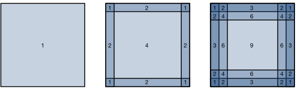
As described above, one tricky issue when applying convolutional layers is that we tend to lose pixels on the perimeter of our image. Consider Fig. 7.3.1 that depicts the pixel utilization as a function of the convolution kernel size and the position within the image. The pixels in the corners are hardly used at all.
위에서 설명한 것처럼 컨볼루션 레이어를 적용할 때 까다로운 문제 중 하나는 이미지 주변에서 픽셀이 손실되는 경향이 있다는 것입니다. 컨벌루션 커널 크기와 이미지 내 위치의 함수로 픽셀 활용도를 나타내는 그림 7.3.1을 고려하십시오. 모서리의 픽셀은 거의 사용되지 않습니다.
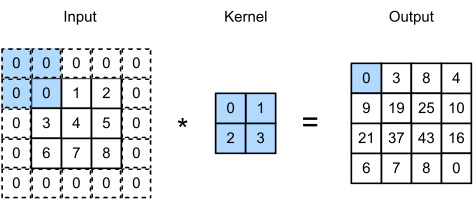
Since we typically use small kernels, for any given convolution, we might only lose a few pixels, but this can add up as we apply many successive convolutional layers. One straightforward solution to this problem is to add extra pixels of filler around the boundary of our input image, thus increasing the effective size of the image. Typically, we set the values of the extra pixels to zero. In Fig. 7.3.2, we pad a 3×3 input, increasing its size to 5×5. The corresponding output then increases to a 4×4 matrix. The shaded portions are the first output element as well as the input and kernel tensor elements used for the output computation: 0×0+0×1+0×2+0×3=0.
우리는 일반적으로 작은 커널을 사용하기 때문에 주어진 컨볼루션에 대해 몇 개의 픽셀만 손실될 수 있지만 이는 많은 연속 컨볼루션 레이어를 적용함에 따라 합산될 수 있습니다. 이 문제에 대한 간단한 해결책 중 하나는 입력 이미지의 경계 주위에 필러 픽셀을 추가하여 이미지의 유효 크기를 늘리는 것입니다. 일반적으로 추가 픽셀 값을 0으로 설정합니다. 그림 7.3.2에서 3×3 입력을 패딩하여 크기를 5×5로 늘립니다. 그러면 해당 출력이 4×4 행렬로 증가합니다. 음영 부분은 첫 번째 출력 요소이자 출력 계산에 사용되는 입력 및 커널 텐서 요소입니다: 0×0+0×1+0×2+0×3=0.
In general, if we add a total of pℎ rows of padding (roughly half on top and half on bottom) and a total of pw columns of padding (roughly half on the left and half on the right), the output shape will be
일반적으로 총 pℎ 행의 패딩(대략 절반은 위쪽, 절반은 아래쪽)과 총 pw 열의 패딩(대략 왼쪽 절반, 오른쪽 절반)을 추가하면 출력 모양은 다음과 같습니다.

This means that the height and width of the output will increase by pℎ and pw, respectively.
이것은 출력의 높이와 너비가 각각 pℎ와 pw만큼 증가한다는 것을 의미합니다.
In many cases, we will want to set pℎ=kℎ−1 and pw=kw−1 to give the input and output the same height and width. This will make it easier to predict the output shape of each layer when constructing the network. Assuming that kℎ is odd here, we will pad pℎ/2 rows on both sides of the height. If kℎ is even, one possibility is to pad ⌈pℎ/2⌉ rows on the top of the input and ⌊pℎ/2⌋ rows on the bottom. We will pad both sides of the width in the same way.
대부분의 경우 입력과 출력에 동일한 높이와 너비를 제공하기 위해 pℎ=kℎ−1 및 pw=kw−1을 설정하려고 합니다. 이렇게 하면 네트워크를 구성할 때 각 레이어의 출력 모양을 더 쉽게 예측할 수 있습니다. 여기서 kℎ가 홀수라고 가정하면 높이 양쪽에 pℎ/2 행을 채울 것입니다. kℎ가 짝수인 경우 한 가지 가능성은 입력 상단의 ⌈pℎ/2⌉ 행과 하단의 ⌊pℎ/2⌋ 행을 채우는 것입니다. 너비의 양쪽을 같은 방식으로 채웁니다.
CNNs commonly use convolution kernels with odd height and width values, such as 1, 3, 5, or 7. Choosing odd kernel sizes has the benefit that we can preserve the dimensionality while padding with the same number of rows on top and bottom, and the same number of columns on left and right.
CNN은 일반적으로 1, 3, 5 또는 7과 같은 홀수 높이 및 너비 값을 가진 컨볼루션 커널을 사용합니다. 홀수 커널 크기를 선택하면 위와 아래에 동일한 수의 행으로 패딩하면서 차원을 보존할 수 있다는 이점이 있습니다. 왼쪽과 오른쪽에 같은 수의 열이 있습니다.
Moreover, this practice of using odd kernels and padding to precisely preserve dimensionality offers a clerical benefit. For any two-dimensional tensor X, when the kernel’s size is odd and the number of padding rows and columns on all sides are the same, producing an output with the same height and width as the input, we know that the output Y[i, j] is calculated by cross-correlation of the input and convolution kernel with the window centered on X[i, j].
더욱이 차원을 정확하게 보존하기 위해 홀수 커널과 패딩을 사용하는 이러한 관행은 사무적인 이점을 제공합니다. 임의의 2차원 텐서 X에 대해 커널의 크기가 홀수이고 모든 면의 패딩 행과 열의 수가 동일하여 입력과 동일한 높이와 너비의 출력을 생성할 때 출력 Y[i , j]는 X[i, j]를 중심으로 하는 윈도우와 입력 및 컨벌루션 커널의 상호 상관에 의해 계산됩니다.
In the following example, we create a two-dimensional convolutional layer with a height and width of 3 and apply 1 pixel of padding on all sides. Given an input with a height and width of 8, we find that the height and width of the output is also 8.
다음 예제에서는 높이와 너비가 3인 2차원 컨볼루션 레이어를 만들고 모든 면에 1픽셀의 패딩을 적용합니다. 높이와 너비가 8인 입력이 주어지면 출력의 높이와 너비도 8임을 알 수 있습니다.
# We define a helper function to calculate convolutions. It initializes the
# convolutional layer weights and performs corresponding dimensionality
# elevations and reductions on the input and output
def comp_conv2d(conv2d, X):
    # (1, 1) indicates that batch size and the number of channels are both 1
    X = X.reshape((1, 1) + X.shape)
    Y = conv2d(X)
    # Strip the first two dimensions: examples and channels
    return Y.reshape(Y.shape[2:])

# 1 row and column is padded on either side, so a total of 2 rows or columns
# are added
conv2d = nn.LazyConv2d(1, kernel_size=3, padding=1)
X = torch.rand(size=(8, 8))
comp_conv2d(conv2d, X).shape- 합성곱(convolution)을 계산하기 위한 도우미 함수를 정의합니다. 이 함수는 컨볼루션 레이어 가중치를 초기화하고 입력과 출력에 대한 차원 변환을 수행합니다.
- (1, 1)은 배치 크기와 채널 수가 모두 1임을 나타냅니다.
- 입력 X를 (1, 1) 크기로 재구성합니다. 이 때, X의 형상에 (1, 1) 차원을 추가합니다.
- 재구성된 입력을 사용하여 컨볼루션 레이어 conv2d를 통과시킵니다.
- 결과인 Y를 반환하기 전에 첫 번째와 두 번째 차원을 제거하여 형상을 조정합니다. 이는 예시와 채널 차원을 제거하는 것을 의미합니다.
- conv2d는 1개의 입력 채널과 3x3 크기의 커널(kernel)을 가지는 컨볼루션 레이어를 정의합니다.
- X는 8x8 크기의 랜덤한 텐서입니다.
- comp_conv2d 함수를 사용하여 conv2d를 X에 적용한 결과의 형상을 확인합니다.

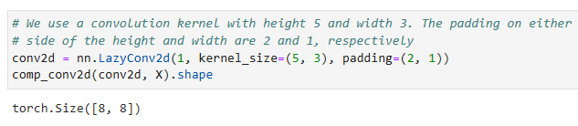
When the height and width of the convolution kernel are different, we can make the output and input have the same height and width by setting different padding numbers for height and width.
컨볼루션 커널의 높이와 너비가 다른 경우 높이와 너비에 다른 패딩 수를 설정하여 출력과 입력의 높이와 너비를 같게 만들 수 있습니다.
# We use a convolution kernel with height 5 and width 3. The padding on either
# side of the height and width are 2 and 1, respectively
conv2d = nn.LazyConv2d(1, kernel_size=(5, 3), padding=(2, 1))
comp_conv2d(conv2d, X).shape- 높이(height)가 5이고 너비(width)가 3인 컨볼루션 커널을 사용합니다. 높이와 너비 양쪽에 대한 패딩(padding)은 각각 2와 1입니다.
- conv2d는 1개의 입력 채널과 5x3 크기의 커널을 가지는 컨볼루션 레이어를 정의합니다.
- 앞선 설명에서 정의한 comp_conv2d 함수를 사용하여 conv2d를 X에 적용한 결과의 형상을 확인합니다.
7.3.2. Stride
When computing the cross-correlation, we start with the convolution window at the upper-left corner of the input tensor, and then slide it over all locations both down and to the right. In the previous examples, we defaulted to sliding one element at a time. However, sometimes, either for computational efficiency or because we wish to downsample, we move our window more than one element at a time, skipping the intermediate locations. This is particularly useful if the convolution kernel is large since it captures a large area of the underlying image.
상호 상관을 계산할 때 입력 텐서의 왼쪽 위 모서리에 있는 컨볼루션 창에서 시작한 다음 모든 위치를 아래로 오른쪽으로 밉니다. 이전 예제에서는 기본적으로 한 번에 하나의 요소를 슬라이딩했습니다. 그러나 때로는 계산 효율성을 위해 또는 다운샘플링을 원하기 때문에 중간 위치를 건너뛰고 한 번에 둘 이상의 요소를 이동합니다. 이는 기본 이미지의 넓은 영역을 캡처하기 때문에 컨볼루션 커널이 큰 경우에 특히 유용합니다.
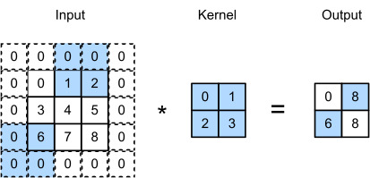
We refer to the number of rows and columns traversed per slide as stride. So far, we have used strides of 1, both for height and width. Sometimes, we may want to use a larger stride. Fig. 7.3.3 shows a two-dimensional cross-correlation operation with a stride of 3 vertically and 2 horizontally. The shaded portions are the output elements as well as the input and kernel tensor elements used for the output computation: 0×0+0×1+1×2+2×3=8, 0×0+6×1+0×2+0×3=6. We can see that when the second element of the first column is generated, the convolution window slides down three rows. The convolution window slides two columns to the right when the second element of the first row is generated. When the convolution window continues to slide two columns to the right on the input, there is no output because the input element cannot fill the window (unless we add another column of padding).
슬라이드당 통과하는 행과 열의 수를 stride(보폭)이라고 합니다. 지금까지 높이와 너비 모두에 1의 보폭(stride)을 사용했습니다. 때로는 더 큰 보폭(stride)을 사용하고 싶을 수도 있습니다. 그림 7.3.3은 스트라이드가 수직으로 3, 수평으로 2인 2차원 교차 상관 연산을 보여줍니다. 음영 부분은 출력 요소와 출력 계산에 사용되는 입력 및 커널 텐서 요소입니다: 0×0+0×1+1×2+2×3=8, 0×0+6×1+0× 2+0×3=6. 첫 번째 열의 두 번째 요소가 생성되면 컨볼루션 창이 세 행 아래로 미끄러지는 것을 볼 수 있습니다. 컨볼루션 창은 첫 번째 행의 두 번째 요소가 생성될 때 오른쪽으로 두 열을 슬라이드합니다. 컨볼루션 창이 입력에서 오른쪽으로 두 열을 계속 슬라이드하면 입력 요소가 창을 채울 수 없기 때문에 출력이 없습니다(다른 패딩 열을 추가하지 않는 한).
In general, when the stride for the height is sℎ and the stride for the width is sw, the output shape is
일반적으로 높이에 대한 stride를 sℎ, 너비에 대한 stride를 sw라고 하면 출력 형태는

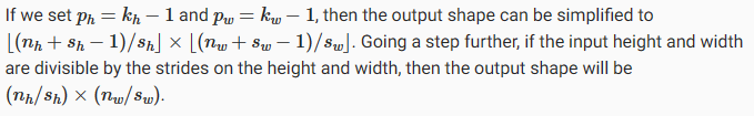
Below, we set the strides on both the height and width to 2, thus halving the input height and width.
pℎ=kℎ−1 및 pw=kw−1로 설정하면 출력 형태를 ⌊(nℎ+sℎ−1)/sℎ⌋×⌊(nw+sw−1)/sw⌋로 단순화할 수 있습니다. 한 단계 더 나아가 입력 높이와 너비를 높이와 너비의 보폭으로 나눌 수 있는 경우 출력 모양은 (nℎ/sℎ)×(nw/sw)가 됩니다.
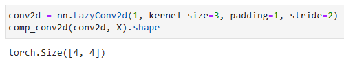
아래에서는 높이와 너비 모두에 대한 보폭을 2로 설정하여 입력 높이와 너비를 반으로 줄입니다.
conv2d = nn.LazyConv2d(1, kernel_size=3, padding=1, stride=2)
comp_conv2d(conv2d, X).shape- 패딩(padding) 값은 1이고 스트라이드(stride) 값은 2인 3x3 커널을 사용하는 컨볼루션 레이어 conv2d를 정의합니다.
- conv2d를 입력 데이터 X에 적용한 결과의 형상을 확인합니다.
- comp_conv2d 함수를 사용하여 컨볼루션 레이어를 적용할 때의 형상 변화를 확인합니다.
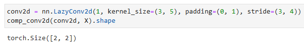
Let’s look at a slightly more complicated example.
조금 더 복잡한 예를 살펴보겠습니다.
conv2d = nn.LazyConv2d(1, kernel_size=(3, 5), padding=(0, 1), stride=(3, 4))
comp_conv2d(conv2d, X).shape- 패딩(padding) 값은 (0, 1)이고 스트라이드(stride) 값은 (3, 4)인 3x5 커널을 사용하는 컨볼루션 레이어 conv2d를 정의합니다.
- conv2d를 입력 데이터 X에 적용한 결과의 형상을 확인합니다.
- comp_conv2d 함수를 사용하여 컨볼루션 레이어를 적용할 때의 형상 변화를 확인합니다.
7.3.3. Summary and Discussion
Padding can increase the height and width of the output. This is often used to give the output the same height and width as the input to avoid undesirable shrinkage of the output. Moreover, it ensures that all pixels are used equally frequently. Typically we pick symmetric padding on both sides of the input height and width. In this case we refer to (pℎ,pw) padding. Most commonly we set pℎ=pw, in which case we simply state that we choose padding p.
패딩은 출력의 높이와 너비를 증가시킬 수 있습니다. 이는 종종 출력이 바람직하지 않게 축소되는 것을 방지하기 위해 입력과 동일한 높이와 너비를 출력에 제공하는 데 사용됩니다. 또한 모든 픽셀이 균등하게 자주 사용되도록 합니다. 일반적으로 입력 높이와 너비의 양쪽에서 대칭 패딩을 선택합니다. 이 경우 (pℎ,pw) 패딩을 참조합니다. 가장 일반적으로 우리는 pℎ=pw를 설정합니다. 이 경우 단순히 패딩 p를 선택한다고 명시합니다.
A similar convention applies to strides. When horizontal stride sℎ and vertical stride sw match, we simply talk about stride s. The stride can reduce the resolution of the output, for example reducing the height and width of the output to only 1/n of the height and width of the input for n>1. By default, the padding is 0 and the stride is 1.
strides에도 유사한 규칙이 적용됩니다. 수평 stride sℎ와 수직 stride sw가 일치하면 간단하게 stride s 라고 합니다. strides은 출력의 해상도를 줄일 수 있습니다. 예를 들어 출력의 높이와 너비를 n>1의 경우 입력의 높이와 너비의 1/n으로만 줄입니다. 기본적으로 패딩은 0이고 스트라이드는 1입니다.
So far all padding that we discussed simply extended images with zeros. This has significant computational benefit since it is trivial to accomplish. Moreover, operators can be engineered to take advantage of this padding implicitly without the need to allocate additional memory. At the same time, it allows CNNs to encode implicit position information within an image, simply by learning where the “whitespace” is. There are many alternatives to zero-padding. Alsallakh et al. (2020) provided an extensive overview of alternatives (albeit without a clear case to use nonzero paddings unless artifacts occur).
지금까지 우리가 논의한 모든 패딩은 단순히 0으로 확장된 이미지입니다. 이것은 달성하기가 쉽지 않기 때문에 계산상 상당한 이점이 있습니다. 또한 연산자는 추가 메모리를 할당할 필요 없이 암시적으로 이 패딩을 활용하도록 설계할 수 있습니다. 동시에 CNN은 단순히 "whitespace"이 어디에 있는지 학습함으로써 이미지 내의 암시적 위치 정보를 인코딩할 수 있습니다. 제로 패딩에 대한 많은 대안이 있습니다. Alsallakhet al. (2020)은 대안에 대한 광범위한 개요를 제공했습니다(아티팩트가 발생하지 않는 한 0이 아닌 패딩을 사용하는 명확한 사례는 없지만).
7.3.4. Exercises
'Dive into Deep Learning > D2L Convolutional Neural Networks (CNN)' 카테고리의 다른 글
| D2L - 8.3. Network in Network (NiN) (0) | 2023.07.11 |
|---|---|
| D2L - 8.2. Networks Using Blocks (VGG) (0) | 2023.07.10 |
| D2L - 8.1. Deep Convolutional Neural Networks (AlexNet) (0) | 2023.07.10 |
| D2L - 8. Modern Convolutional Neural Networks (0) | 2023.07.10 |
| D2L - 7.6. Convolutional Neural Networks (LeNet) (0) | 2023.07.09 |
| D2L - 7.5. Pooling (1) | 2023.07.09 |
| D2L - 7.4. Multiple Input and Multiple Output Channels (0) | 2023.07.09 |
| D2L - 7.2. Convolutions for Images (0) | 2023.07.09 |
| D2L - 7.1. From Fully Connected Layers to Convolutions (0) | 2023.07.09 |
| D2L - 7. Convolutional Neural Networks (0) | 2023.07.09 |