

8.2. Networks Using Blocks (VGG) — Dive into Deep Learning 1.0.0-beta0 documentation (d2l.ai)
8.2. Networks Using Blocks (VGG) — Dive into Deep Learning 1.0.0-beta0 documentation
d2l.ai
8.2. Networks Using Blocks (VGG)
While AlexNet offered empirical evidence that deep CNNs can achieve good results, it did not provide a general template to guide subsequent researchers in designing new networks. In the following sections, we will introduce several heuristic concepts commonly used to design deep networks.
AlexNet은 심층 CNN이 좋은 결과를 달성할 수 있다는 경험적 증거를 제공했지만 후속 연구원이 새로운 네트워크를 설계하는 데 도움이 되는 일반적인 템플릿은 제공하지 않았습니다. 다음 섹션에서는 딥 네트워크를 설계하는 데 일반적으로 사용되는 몇 가지 휴리스틱 개념을 소개합니다.
Progress in this field mirrors that of VLSI (very large scale integration) in chip design where engineers moved from placing transistors to logical elements to logic blocks (Mead, 1980). Similarly, the design of neural network architectures has grown progressively more abstract, with researchers moving from thinking in terms of individual neurons to whole layers, and now to blocks, repeating patterns of layers. A decade later, this has now progressed to researchers using entire trained models to repurpose them for different, albeit related, tasks. Such large pretrained models are typically called foundation models (Bommasani et al., 2021).
이 분야의 발전은 엔지니어가 트랜지스터 배치에서 논리 요소, 논리 블록으로 이동한 칩 설계의 VLSI(초대규모 통합)를 반영합니다(Mead, 1980). 유사하게, 신경망 구조의 디자인은 연구자들이 개별 뉴런의 관점에서 생각하는 것에서 전체 층으로, 이제는 층의 패턴을 반복하는 블록으로 이동하면서 점점 더 추상적으로 성장했습니다. 10년 후, 이것은 비록 관련이 있긴 하지만 다른 작업을 위해 용도를 변경하기 위해 전체 훈련된 모델을 사용하는 연구자에게 발전했습니다. 이러한 대규모 사전 훈련 모델은 일반적으로 foundation models이라고 합니다(Bommasani et al., 2021).
Back to network design. The idea of using blocks first emerged from the Visual Geometry Group (VGG) at Oxford University, in their eponymously-named VGG network (Simonyan and Zisserman, 2014). It is easy to implement these repeated structures in code with any modern deep learning framework by using loops and subroutines.
네트워크 설계로 돌아갑니다. 블록을 사용한다는 아이디어는 옥스포드 대학의 VGG(Visual Geometry Group)에서 VGG 네트워크라는 이름으로 처음 등장했습니다(Simonyan and Zisserman, 2014). 루프와 서브루틴을 사용하여 최신 딥 러닝 프레임워크를 사용하여 코드에서 이러한 반복 구조를 쉽게 구현할 수 있습니다.
Vissual Geometry Group (VGG) 란?
The Visual Geometry Group (VGG) is a convolutional neural network architecture that was proposed by the Visual Geometry Group at the University of Oxford. VGG is known for its simplicity and effectiveness in image classification tasks.
Visual Geometry Group (VGG)은 옥스퍼드 대학교의 Visual Geometry Group에서 제안한 합성곱 신경망 구조입니다. VGG는 이미지 분류 작업에서의 간결성과 효율성으로 알려져 있습니다.
The VGG architecture consists of a series of convolutional layers, followed by max-pooling layers, and finally fully connected layers. The key characteristic of VGG is that it uses a stack of small-sized convolutional filters (3x3) with a stride of 1, and always uses the same padding to maintain the spatial resolution of the feature maps. This design choice allows VGG to learn hierarchical representations of visual patterns at different scales.
VGG 아키텍처는 일련의 합성곱 레이어, 맥스 풀링 레이어, 그리고 완전 연결 레이어로 구성됩니다. VGG의 주요 특징은 스트라이드 1과 동일한 패딩을 사용하여 작은 크기의 합성곱 필터(3x3)를 스택 형태로 사용한다는 점입니다. 이러한 설계 선택은 VGG가 다양한 스케일의 시각적 패턴에 대한 계층적인 표현을 학습할 수 있도록 합니다.
The original VGG network comes in different variants, such as VGG16 and VGG19, which differ in the number of layers. VGG16 has 16 layers, including 13 convolutional layers and 3 fully connected layers, while VGG19 has 19 layers. The deeper architectures allow VGG to capture more complex features and achieve higher accuracy on image classification tasks.
원래의 VGG 네트워크에는 VGG16과 VGG19와 같은 여러 가지 변형이 있으며, 이는 레이어의 수에 차이가 있습니다. VGG16은 13개의 합성곱 레이어와 3개의 완전 연결 레이어를 포함하여 총 16개의 레이어로 구성되어 있으며, VGG19는 19개의 레이어로 이루어져 있습니다. 더 깊은 아키텍처를 통해 VGG는 더 복잡한 특징을 학습하고 이미지 분류 작업에서 더 높은 정확도를 달성할 수 있습니다.
VGG networks have been widely used as a benchmark architecture for various computer vision tasks, including image classification, object detection, and image segmentation. They have also influenced the design of subsequent convolutional neural network architectures.
VGG 네트워크는 이미지 분류, 객체 검출, 이미지 세그멘테이션 등 다양한 컴퓨터 비전 작업에서 벤치마크 아키텍처로 널리 사용되었습니다. 또한, VGG는 후속 합성곱 신경망 아키텍처의 설계에도 영향을 미쳤습니다.
Overall, VGG is known for its simplicity, strong performance, and ability to learn expressive representations of visual data, making it a popular choice in the field of deep learning for computer vision tasks.
전반적으로 VGG는 간결성, 강력한 성능, 시각적 데이터의 표현 학습 능력을 갖춘 특징으로 인해 컴퓨터 비전 작업에서 인기 있는 선택지입니다.
VGGNet
* Convolution + ReLU, max poling, fully connected + ReLU, softmax
* 3X3 convolution -> Max Pooling을 계속 반복함 => 이 반복하는 구간을 Block 이라고 함 (VGG Block)
블럭 내에서 Convolution을 몇번 반복 할 것인가? 그리고 필터는 몇개를 쓸 것인가? 를 결정해야 함
* Receptive Field : Convolution을 많이 반복 할 수록 더 큰 영역의 원본 이미지를 처리하게 된다.
import torch
from torch import nn
from d2l import torch as d2l
8.2.1. VGG Blocks
The basic building block of CNNs is a sequence of the following: (i) a convolutional layer with padding to maintain the resolution, (ii) a nonlinearity such as a ReLU, (iii) a pooling layer such as max-pooling to reduce the resolution. One of the problems with this approach is that the spatial resolution decreases quite rapidly. In particular, this imposes a hard limit of log2d convolutional layers on the network before all dimensions (d) are used up. For instance, in the case of ImageNet, it would be impossible to have more than 8 convolutional layers in this way.
CNN의 기본 빌딩 블록은 (i) 해상도를 유지하기 위한 패딩이 있는 컨볼루션 레이어, (ii) ReLU와 같은 비선형성, (iii) 해결. 이 접근법의 문제점 중 하나는 공간 해상도가 매우 빠르게 감소한다는 것입니다. 특히 이것은 모든 차원(d)이 사용되기 전에 네트워크에서 log2d 컨벌루션 계층의 엄격한 제한을 부과합니다. 예를 들어 ImageNet의 경우 이런 방식으로 8개 이상의 컨볼루션 레이어를 갖는 것은 불가능합니다.
The key idea of Simonyan and Zisserman (2014) was to use multiple convolutions in between downsampling via max-pooling in the form of a block. They were primarily interested in whether deep or wide networks perform better. For instance, the successive application of two 3×3 convolutions touches the same pixels as a single 5×5 convolution does. At the same time, the latter uses approximately as many parameters (25⋅c2) as three 3×3 convolutions do (3⋅9⋅c2). In a rather detailed analysis they showed that deep and narrow networks significantly outperform their shallow counterparts. This set deep learning on a quest for ever deeper networks with over 100 layers for typical applications. Stacking 3×3 convolutions has become a gold standard in later deep networks (a design decision only to be revisited recently by Liu et al. (2022)). Consequently, fast implementations for small convolutions have become a staple on GPUs (Lavin and Gray, 2016).
Simonyan과 Zisserman(2014)의 핵심 아이디어는 블록 형태의 최대 풀링을 통해 다운샘플링 사이에 다중 컨벌루션을 사용하는 것이었습니다. 그들은 주로 깊은 네트워크 또는 넓은 네트워크가 더 잘 수행되는지 여부에 관심이 있었습니다. 예를 들어 두 개의 3×3 컨볼루션을 연속적으로 적용하면 단일 5×5 컨볼루션과 동일한 픽셀에 닿습니다. 동시에 후자는 대략 3개의 3×3 컨볼루션(3⋅9⋅c2)만큼 많은 매개변수(25⋅c2)를 사용합니다. 다소 상세한 분석에서 그들은 깊고 좁은 네트워크가 얕은 네트워크보다 훨씬 뛰어난 성능을 보인다는 것을 보여주었습니다. 이는 일반적인 애플리케이션을 위한 100개 이상의 레이어가 있는 더 깊은 네트워크에 대한 탐구에 대한 딥 러닝을 설정합니다. Stacking 3×3 Convolution은 이후 딥 네트워크에서 금본위제가 되었습니다(Liu et al.(2022)이 최근에 재검토한 디자인 결정). 결과적으로 작은 컨볼루션을 위한 빠른 구현은 GPU의 필수 요소가 되었습니다(Lavin and Gray, 2016).
Back to VGG: a VGG block consists of a sequence of convolutions with 3×3 kernels with padding of 1 (keeping height and width) followed by a 2×2 max-pooling layer with stride of 2 (halving height and width after each block). In the code below, we define a function called vgg_block to implement one VGG block.
VGG로 돌아가서: VGG 블록은 패딩이 1(높이와 너비 유지)인 3×3 커널과 보폭이 2인 2×2 최대 풀링 레이어(각 블록 후 높이와 너비를 반으로 줄임)가 있는 일련의 컨볼루션으로 구성됩니다. ). 아래 코드에서는 하나의 VGG 블록을 구현하기 위해 vgg_block이라는 함수를 정의합니다.
The function below takes two arguments, corresponding to the number of convolutional layers num_convs and the number of output channels num_channels.
아래 함수는 컨벌루션 레이어의 수 num_convs와 출력 채널의 수 num_channels에 해당하는 두 개의 인수를 사용합니다.
def vgg_block(num_convs, out_channels):
    layers = []
    for _ in range(num_convs):
        layers.append(nn.LazyConv2d(out_channels, kernel_size=3, padding=1))
        layers.append(nn.ReLU())
    layers.append(nn.MaxPool2d(kernel_size=2,stride=2))
    return nn.Sequential(*layers)
위의 코드는 VGG 블록을 생성하는 함수인 vgg_block을 정의합니다. VGG 블록은 일련의 합성곱 레이어, 활성화 함수(ReLU), 그리고 맥스 풀링 레이어로 구성됩니다.
함수의 인자로는 num_convs와 out_channels가 있습니다. num_convs는 VGG 블록 내에서 반복되는 합성곱 레이어의 개수를 나타냅니다. out_channels는 각 합성곱 레이어의 출력 채널 수를 의미합니다.
함수는 빈 리스트인 layers를 생성한 후, num_convs만큼의 반복문을 실행합니다. 각 반복에서는 합성곱 레이어(nn.LazyConv2d)와 활성화 함수(ReLU)를 순서대로 layers 리스트에 추가합니다.
반복문이 끝난 후에는 맥스 풀링 레이어(nn.MaxPool2d)를 layers 리스트에 추가합니다. 맥스 풀링 레이어는 입력의 크기를 절반으로 줄이는 역할을 수행합니다.
마지막으로, layers 리스트의 모든 요소를 nn.Sequential을 사용하여 순차적으로 결합한 후 반환합니다. 이렇게 생성된 VGG 블록은 더 큰 VGG 네트워크에서 사용될 수 있습니다.
8.2.2. VGG Network
Like AlexNet and LeNet, the VGG Network can be partitioned into two parts: the first consisting mostly of convolutional and pooling layers and the second consisting of fully connected layers that are identical to those in AlexNet. The key difference is that the convolutional layers are grouped in nonlinear transformations that leave the dimensonality unchanged, followed by a resolution-reduction step, as depicted in Fig. 8.2.1.
AlexNet 및 LeNet과 마찬가지로 VGG 네트워크는 두 부분으로 나눌 수 있습니다. 첫 번째 부분은 주로 컨벌루션 및 풀링 레이어로 구성되고 두 번째 부분은 AlexNet의 레이어와 동일한 완전히 연결된 레이어로 구성됩니다. 주요 차이점은 그림 8.2.1에 묘사된 것처럼 컨벌루션 레이어가 차원을 변경하지 않고 해상도 감소 단계가 뒤따르는 비선형 변환으로 그룹화된다는 것입니다.
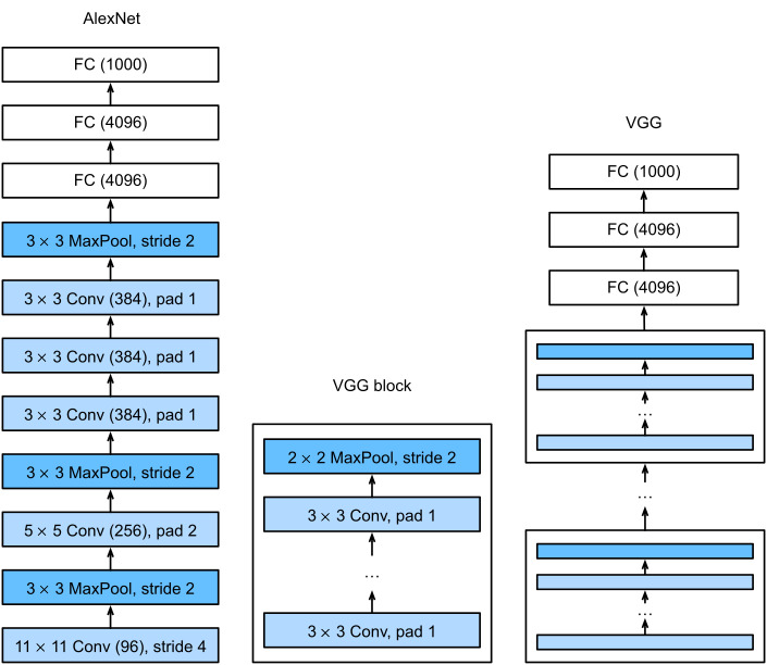
The convolutional part of the network connects several VGG blocks from Fig. 8.2.1 (also defined in the vgg_block function) in succession. This grouping of convolutions is a pattern that has remained almost unchanged over the past decade, although the specific choice of operations has undergone considerable modifications. The variable conv_arch consists of a list of tuples (one per block), where each contains two values: the number of convolutional layers and the number of output channels, which are precisely the arguments required to call the vgg_block function. As such, VGG defines a family of networks rather than just a specific manifestation. To build a specific network we simply iterate over arch to compose the blocks.
네트워크의 컨벌루션 부분은 그림 8.2.1(vgg_block 함수에서도 정의됨)의 여러 VGG 블록을 연속적으로 연결합니다. 이 컨볼루션 그룹화는 특정 작업 선택이 상당한 수정을 거쳤지만 지난 10년 동안 거의 변경되지 않은 패턴입니다. 변수 conv_arch는 튜플 목록(블록당 하나)으로 구성되며 각 튜플에는 vgg_block 함수를 호출하는 데 필요한 정확히 인수인 컨벌루션 레이어 수와 출력 채널 수라는 두 가지 값이 포함됩니다. 이와 같이 VGG는 특정 표현이 아닌 네트워크 제품군을 정의합니다. 특정 네트워크를 구축하기 위해 우리는 단순히 블록을 구성하기 위해 아치를 반복합니다.
class VGG(d2l.Classifier):
    def __init__(self, arch, lr=0.1, num_classes=10):
        super().__init__()
        self.save_hyperparameters()
        conv_blks = []
        for (num_convs, out_channels) in arch:
            conv_blks.append(vgg_block(num_convs, out_channels))
        self.net = nn.Sequential(
            *conv_blks, nn.Flatten(),
            nn.LazyLinear(4096), nn.ReLU(), nn.Dropout(0.5),
            nn.LazyLinear(4096), nn.ReLU(), nn.Dropout(0.5),
            nn.LazyLinear(num_classes))
        self.net.apply(d2l.init_cnn)
위의 코드는 VGG 모델을 정의하는 VGG 클래스를 나타냅니다. VGG 클래스는 d2l.Classifier 클래스를 상속받습니다.
클래스의 __init__ 메서드에서는 VGG 모델의 구조를 정의하고 초기화를 수행합니다. arch 인자는 VGG 모델의 구조를 나타내는 리스트로, 각 요소는 (num_convs, out_channels) 형태의 튜플입니다. num_convs는 VGG 블록 내에서 반복되는 합성곱 레이어의 개수를 의미하고, out_channels는 각 합성곱 레이어의 출력 채널 수를 나타냅니다.
conv_blks 리스트를 생성한 후, arch를 순회하면서 각각의 (num_convs, out_channels)에 대해 vgg_block 함수를 호출하여 VGG 블록을 생성하고 conv_blks 리스트에 추가합니다.
그 다음, nn.Sequential을 사용하여 conv_blks 리스트에 저장된 VGG 블록들을 순차적으로 결합합니다. 이후에는 nn.Flatten 레이어를 추가하여 다차원 텐서를 1차원으로 평탄화합니다.
마지막으로, fully connected 레이어를 추가합니다. nn.LazyLinear은 지연 초기화된 선형 레이어를 나타냅니다. VGG 모델의 fully connected 레이어는 두 개의 4096 차원 레이어와 마지막에 출력 클래스 수에 해당하는 레이어로 구성됩니다. 활성화 함수로는 ReLU를 사용하고, dropout을 적용하여 모델의 일반화 능력을 향상시킵니다.
마지막으로, self.net에 적용된 d2l.init_cnn 함수를 사용하여 모델의 가중치를 초기화합니다. 이렇게 정의된 VGG 클래스는 이미지 분류 작업에 사용될 수 있는 VGG 모델을 생성합니다.
Sequential — PyTorch 2.0 documentation
Sequential — PyTorch 2.0 documentation
Shortcuts
pytorch.org
LazyLinear — PyTorch 2.0 documentation
LazyLinear — PyTorch 2.0 documentation
Shortcuts
pytorch.org
The original VGG network had 5 convolutional blocks, among which the first two have one convolutional layer each and the latter three contain two convolutional layers each. The first block has 64 output channels and each subsequent block doubles the number of output channels, until that number reaches 512. Since this network uses 8 convolutional layers and 3 fully connected layers, it is often called VGG-11.
원래 VGG 네트워크에는 5개의 컨볼루션 블록이 있으며, 그 중 처음 2개는 각각 1개의 컨볼루션 레이어를, 나머지 3개는 각각 2개의 컨볼루션 레이어를 포함합니다. 첫 번째 블록에는 64개의 출력 채널이 있고 각 후속 블록은 그 수가 512에 도달할 때까지 출력 채널 수를 두 배로 늘립니다. 이 네트워크는 8개의 컨볼루션 레이어와 3개의 완전 연결 레이어를 사용하므로 종종 VGG-11이라고 합니다.
VGG(arch=((1, 64), (1, 128), (2, 256), (2, 512), (2, 512))).layer_summary(
    (1, 1, 224, 224))
위의 코드는 VGG 모델의 구조를 정의한 후, layer_summary 메서드를 사용하여 각 레이어의 출력 형태를 요약하는 예시입니다.
VGG(arch=((1, 64), (1, 128), (2, 256), (2, 512), (2, 512)))는 VGG 모델을 생성하는데, arch 인자로 (num_convs, out_channels) 형태의 튜플로 이루어진 리스트를 전달합니다. 각 튜플은 VGG 블록 내에서의 합성곱 레이어 개수와 출력 채널 수를 나타냅니다.
그리고 layer_summary 메서드를 호출하여 모델의 레이어를 요약합니다. 이 메서드는 주어진 입력 형태 (1, 1, 224, 224)에 대해 각 레이어의 출력 형태를 출력합니다. 이를 통해 모델의 구조와 레이어 간의 입력-출력 관계를 파악할 수 있습니다.
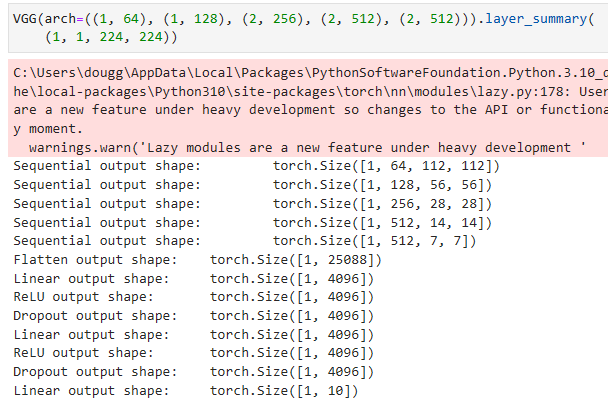
As you can see, we halve height and width at each block, finally reaching a height and width of 7 before flattening the representations for processing by the fully connected part of the network. Simonyan and Zisserman (2014) described several other variants of VGG. In fact, it has become the norm to propose families of networks with different speed-accuracy trade-off when introducing a new architecture.
보시다시피, 우리는 각 블록에서 높이와 너비를 절반으로 줄였고, 완전히 연결된 네트워크 부분에서 처리하기 위해 표현을 평면화하기 전에 마침내 높이와 너비가 7에 도달했습니다. Simonyan과 Zisserman(2014)은 VGG의 몇 가지 다른 변종을 설명했습니다. 실제로 새로운 아키텍처를 도입할 때 서로 다른 속도-정확도 트레이드 오프를 가진 네트워크 제품군을 제안하는 것이 일반적이 되었습니다.
8.2.3. Training
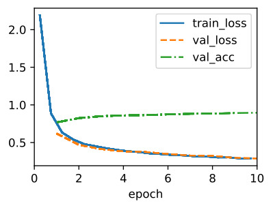
Since VGG-11 is computationally more demanding than AlexNet we construct a network with a smaller number of channels. This is more than sufficient for training on Fashion-MNIST. The model training process is similar to that of AlexNet in Section 8.1. Again observe the close match between validation and training loss, suggesting only a small amount of overfitting.
8.1. Deep Convolutional Neural Networks (AlexNet) — Dive into Deep Learning 1.0.0-beta0 documentation
d2l.ai
VGG-11은 AlexNet보다 계산적으로 더 까다롭기 때문에 더 적은 수의 채널로 네트워크를 구성합니다. 이것은 Fashion-MNIST 교육에 충분합니다. 모델 학습 과정은 섹션 8.1의 AlexNet과 유사합니다. 유효성 검사와 훈련 손실 사이의 밀접한 일치를 다시 관찰하여 소량의 과적합만 제안합니다.
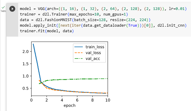
model = VGG(arch=((1, 16), (1, 32), (2, 64), (2, 128), (2, 128)), lr=0.01)
trainer = d2l.Trainer(max_epochs=10, num_gpus=1)
data = d2l.FashionMNIST(batch_size=128, resize=(224, 224))
model.apply_init([next(iter(data.get_dataloader(True)))[0]], d2l.init_cnn)
trainer.fit(model, data)
위의 코드는 VGG 모델을 생성하고 훈련하는 과정을 나타냅니다.
model = VGG(arch=((1, 16), (1, 32), (2, 64), (2, 128), (2, 128)), lr=0.01)은 VGG 모델을 생성합니다. arch 인자에는 VGG 블록 내의 합성곱 레이어 개수와 출력 채널 수를 지정한 튜플로 이루어진 리스트를 전달합니다. 또한, 학습률 lr도 지정합니다.
trainer = d2l.Trainer(max_epochs=10, num_gpus=1)은 훈련에 필요한 Trainer 객체를 생성합니다. max_epochs는 최대 에폭 수를, num_gpus는 사용할 GPU 개수를 나타냅니다.
data = d2l.FashionMNIST(batch_size=128, resize=(224, 224))는 FashionMNIST 데이터셋을 로드하고 전처리합니다. 배치 크기 batch_size와 이미지 크기 resize를 지정합니다.
model.apply_init([next(iter(data.get_dataloader(True)))[0]], d2l.init_cnn)은 모델의 가중치를 초기화합니다. 데이터로더에서 첫 번째 배치를 가져와서 입력으로 사용하고, d2l.init_cnn 함수를 통해 가중치를 초기화합니다.
trainer.fit(model, data)은 모델을 훈련합니다. Trainer 객체를 사용하여 지정된 데이터셋을 사용하여 모델을 학습하고, 주어진 에폭 수만큼 반복적으로 훈련을 진행합니다.
8.2.4. Summary
One might argue that VGG is the first truly modern convolutional neural network. While AlexNet introduced many of the components of what make deep learning effective at scale, it is VGG that arguably introduced key properties such as blocks of multiple convolutions and a preference for deep and narrow networks. It is also the first network that is actually an entire family of similarly parametrized models, giving the practitioner ample trade-off between complexity and speed. This is also the place where modern deep learning frameworks shine. It is no longer necessary to generate XML config files to specify a network but rather, to assemble said networks through simple Python code.
VGG가 최초의 진정한 현대 컨볼루션 신경망이라고 주장할 수도 있습니다. AlexNet은 딥 러닝을 대규모로 효과적으로 만드는 많은 구성 요소를 도입했지만 VGG는 여러 컨볼루션의 블록 및 깊고 좁은 네트워크에 대한 선호와 같은 주요 속성을 도입했다고 주장할 수 있습니다. 이것은 실제로 유사하게 매개변수화된 모델의 전체 제품군인 최초의 네트워크로, 실무자에게 복잡성과 속도 사이에서 충분한 절충안을 제공합니다. 이것은 또한 최신 딥 러닝 프레임워크가 빛나는 곳이기도 합니다. 더 이상 네트워크를 지정하기 위해 XML 구성 파일을 생성할 필요가 없으며 간단한 Python 코드를 통해 해당 네트워크를 조립할 수 있습니다.
Very recently ParNet (Goyal et al., 2021) demonstrated that it is possible to achieve competitive performance using a much more shallow architecture through a large number of parallel computations. This is an exciting development and there’s hope that it will influence architecture designs in the future. For the remainder of the chapter, though, we will follow the path of scientific progress over the past decade.
아주 최근에 ParNet(Goyal et al., 2021)은 많은 수의 병렬 계산을 통해 훨씬 더 얕은 아키텍처를 사용하여 경쟁력 있는 성능을 달성할 수 있음을 보여주었습니다. 이것은 흥미로운 발전이며 미래의 건축 디자인에 영향을 미칠 것이라는 희망이 있습니다. 하지만 이 장의 나머지 부분에서는 지난 10년 동안의 과학적 진보의 길을 따라갈 것입니다.
8.2.5. Exercises
- Compared with AlexNet, VGG is much slower in terms of computation, and it also needs more GPU memory.
- Compare the number of parameters needed for AlexNet and VGG.
- Compare the number of floating point operations used in the convolutional layers and in the fully connected layers.
- How could you reduce the computational cost created by the fully connected layers?
- When displaying the dimensions associated with the various layers of the network, we only see the information associated with 8 blocks (plus some auxiliary transforms), even though the network has 11 layers. Where did the remaining 3 layers go?
- Use Table 1 in the VGG paper (Simonyan and Zisserman, 2014) to construct other common models, such as VGG-16 or VGG-19.
- Upsampling the resolution in Fashion-MNIST by a factor of 8 from 28×28 to 224×224 dimensions is very wasteful. Try modifying the network architecture and resolution conversion, e.g., to 56 or to 84 dimensions for its input instead. Can you do so without reducing the accuracy of the network? Consider the VGG paper (Simonyan and Zisserman, 2014) for ideas on adding more nonlinearities prior to downsampling.
'Dive into Deep Learning > D2L Convolutional Neural Networks (CNN)' 카테고리의 다른 글
| D2L - 8.7. Densely Connected Networks (DenseNet) (0) | 2023.07.18 |
|---|---|
| D2L - 8.6. Residual Networks (ResNet) and ResNeXt (0) | 2023.07.18 |
| D2L - 8.5. Batch Normalization (0) | 2023.07.18 |
| D2L - 8.4. Multi-Branch Networks (GoogLeNet) (0) | 2023.07.18 |
| D2L - 8.3. Network in Network (NiN) (0) | 2023.07.11 |
| D2L - 8.1. Deep Convolutional Neural Networks (AlexNet) (0) | 2023.07.10 |
| D2L - 8. Modern Convolutional Neural Networks (0) | 2023.07.10 |
| D2L - 7.6. Convolutional Neural Networks (LeNet) (0) | 2023.07.09 |
| D2L - 7.5. Pooling (1) | 2023.07.09 |
| D2L - 7.4. Multiple Input and Multiple Output Channels (0) | 2023.07.09 |