

https://d2l.ai/chapter_convolutional-modern/resnet.html
8.6. Residual Networks (ResNet) and ResNeXt — Dive into Deep Learning 1.0.0-beta0 documentation
d2l.ai
8.6. Residual Networks (ResNet) and ResNeXt
점점 더 깊은 네트워크를 설계함에 따라 레이어 추가가 어떻게 네트워크의 복잡성과 표현력을 증가시킬 수 있는지 이해하는 것이 필수적입니다. 훨씬 더 중요한 것은 레이어를 추가하면 네트워크가 단순히 다른 것보다 훨씬 더 표현력 있게 만드는 네트워크를 설계하는 능력입니다. 진전을 이루려면 약간의 수학이 필요합니다.
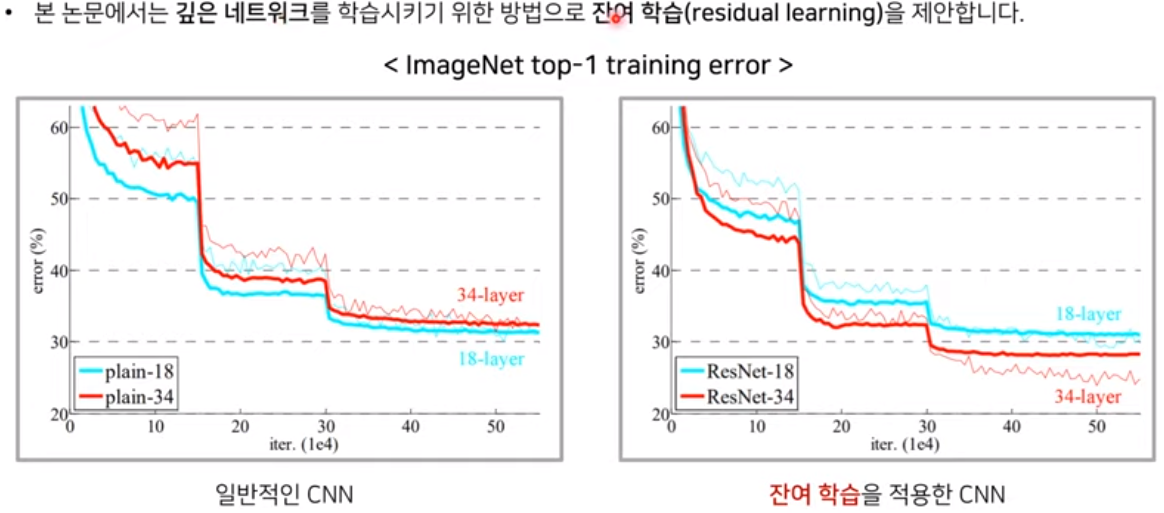
이때부터 에러율이 사람보다 낮아졌다.
Layer가 깊어질 수록 성능이 좋아지지 않는 이유는 기울기 소실(degradation) 문제 때문임
Conversion block과 Identification block으로 나뉨
아래 방식으로 Vanishing Gradient를 해결 (backpropagate 시 미분값이 덜 적어짐)
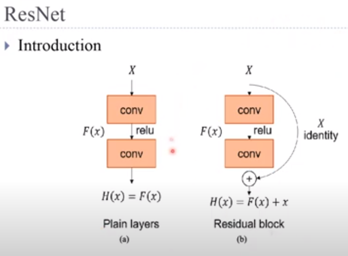

Residual learning framework : input 값을 output 값에 더애서 다음 layer의 input 값으로 넣어 줌
: 앞 단계 (layer들)에서 학습된 정보에 현재 layer에서 학습된 정보를 더해 줌으로서 현재 layer까지 학습된 모든 정보를 다음 layer에 전달할 수 있음. ==> layer가 깊어 질 수록 성능이 더 좋아 짐
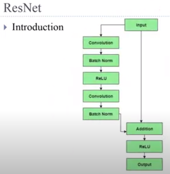
Conv와 ReLu 사이에 batch normalization 사용함
이 논문에 나오는 Identity란?
In the context of ResNet's thesis, 'identity' refers to the concept of using the identity mapping as one of the building blocks in the deep neural network architecture. In a traditional deep neural network, each layer is typically responsible for learning a specific transformation from its input to its output. However, as the network becomes deeper, it may face challenges in learning these transformations effectively, leading to issues like vanishing gradients and degradation of performance.
ResNet 논문에서의 'identity(항등)'은 딥 뉴럴 네트워크 아키텍처의 구성 요소 중 하나로서 항등 매핑(identity mapping)을 사용하는 개념을 의미합니다. 전통적인 딥 뉴럴 네트워크에서 각 레이어는 일반적으로 입력에서 출력으로의 특정 변환을 학습하는 것으로 구성됩니다. 그러나 네트워크가 깊어질수록 이러한 변환을 효과적으로 학습하는 데 어려움을 겪을 수 있으며, 이로 인해 사라지는 그래디언트와 성능 저하 등의 문제가 발생할 수 있습니다.
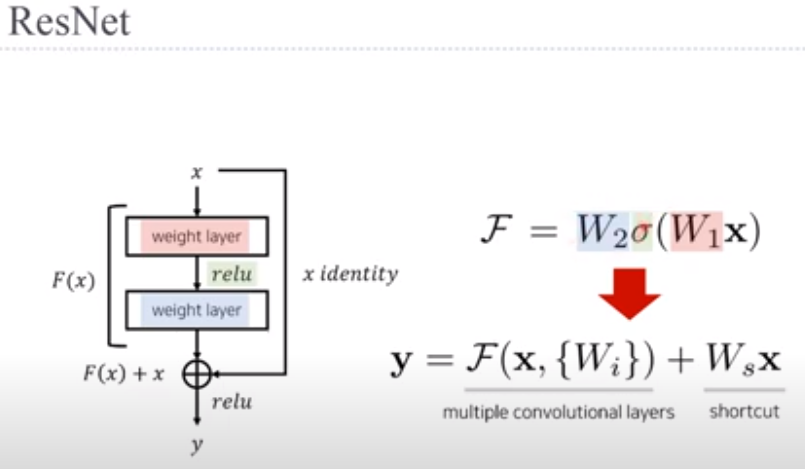
The ResNet architecture introduces the concept of residual blocks, which allow the network to learn the residual (the difference between the desired output and the input) instead of the entire transformation. The key idea is to define the mapping of each layer as the sum of the original input (identity mapping) and the learned residual mapping. This way, the network can be encouraged to learn small changes to the input data, making it easier for the model to optimize and preventing the vanishing gradient problem.
ResNet 아키텍처는 잔차 블록(residual block) 개념을 도입하여 네트워크가 전체 변환 대신 잔차(입력과 원하는 출력 간의 차이)를 학습하도록 할 수 있습니다. 주요 아이디어는 각 레이어의 매핑을 원래 입력(항등 매핑)과 학습된 잔차 매핑의 합으로 정의하는 것입니다. 이렇게 함으로써 네트워크는 입력 데이터에 대한 작은 변경을 학습하도록 장려되며, 모델이 최적화하기 쉽고 사라지는 그래디언트 문제를 방지할 수 있습니다.
By introducing identity mappings, the authors of the ResNet paper proposed that deep neural networks could be trained effectively even with hundreds or thousands of layers, allowing them to achieve state-of-the-art performance on various image recognition tasks.
항등 매핑을 도입함으로써 ResNet 논문의 저자들은 수백 개 또는 수천 개의 레이어를 가진 깊은 딥 뉴럴 네트워크도 효과적으로 학습할 수 있다고 제안하였으며, 이를 통해 다양한 이미지 인식 작업에서 최첨단 성능을 달성할 수 있었습니다.
In summary, 'identity' in ResNet's thesis refers to the direct mapping from input to output, and the use of identity mappings as a key component in the residual blocks helps address the optimization challenges associated with very deep neural networks.
요약하면, ResNet 논문에서의 'identity(항등)'은 입력에서 출력으로의 직접적인 매핑을 의미하며, 이러한 항등 매핑을 잔차 블록의 주요 구성 요소로 사용함으로써 매우 깊은 딥 뉴럴 네트워크와 관련된 최적화 문제를 해결하는 데 도움이 되었습니다.
ResNet은 각 layer별로 크게 차이가 나지 않게 함으로서 천천히 작업을 진행하도록 함
차이만 학습하는 것이 ResNet임.
import torch
from torch import nn
from torch.nn import functional as F
from d2l import torch as d2l
위 코드는 PyTorch와 deep learning 라이브러리인 d2l을 사용하는데 필요한 모듈들을 임포트하는 부분입니다.
- import torch: PyTorch 라이브러리를 임포트합니다. PyTorch는 딥러닝 연구 및 개발을 위한 강력한 프레임워크로, 텐서 조작, 모델 구성, 학습 등에 사용됩니다.
- from torch import nn: PyTorch의 nn 모듈에서 nn이라는 클래스를 가져옵니다. nn 모듈은 신경망 구성 요소를 정의하는 데 사용되며, 여기서는 nn.Module을 확장한 다양한 층과 모듈들을 사용할 수 있습니다.
- from torch.nn import functional as F: PyTorch의 nn.functional 모듈에서 F라는 별칭을 가져옵니다. nn.functional 모듈은 신경망의 활성화 함수, 손실 함수 등과 같은 함수적인 기능들을 제공합니다.
- from d2l import torch as d2l: d2l이라는 패키지에서 torch라는 이름의 모듈을 가져옵니다. 이것은 d2l 패키지에서 torch와 관련된 함수들을 사용할 수 있게 해줍니다. d2l은 Dive into Deep Learning (D2L) 교재의 코드를 위한 도우미 라이브러리로, 딥러닝 학습에 도움이 되는 함수들과 유틸리티들을 제공합니다.
이러한 모듈들을 임포트하면 딥러닝 모델을 구성하고 학습하는 데 필요한 다양한 기능들을 사용할 수 있습니다.
8.6.1. Function Classes
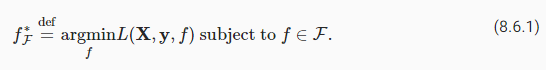
Consider F, the class of functions that a specific network architecture (together with learning rates and other hyperparameter settings) can reach. That is, for all f∈F there exists some set of parameters (e.g., weights and biases) that can be obtained through training on a suitable dataset. Let’s assume that f∗ is the “truth” function that we really would like to find. If it is in F, we are in good shape but typically we will not be quite so lucky. Instead, we will try to find somefF∗ which is our best bet within F. For instance, given a dataset with features X and labels y, we might try finding it by solving the following optimization problem:
특정 네트워크 아키텍처(학습률 및 기타 하이퍼파라미터 설정과 함께)가 도달할 수 있는 함수 클래스인 F를 고려하십시오. 즉, 모든 f∈F에 대해 적절한 데이터 세트에 대한 훈련을 통해 얻을 수 있는 일부 매개변수 세트(예: 가중치 및 편향)가 존재합니다. f*가 우리가 정말로 찾고자 하는 "진실" 함수라고 가정해 봅시다. 그것이 F에 있다면 우리는 좋은 상태이지만 일반적으로 우리는 그렇게 운이 좋지 않을 것입니다. 대신, 우리는 F 내에서 최선의 선택인 fF*를 찾으려고 노력할 것입니다. 예를 들어, 특성 X와 레이블 y가 있는 데이터 세트가 주어지면 다음 최적화 문제를 해결하여 찾을 수 있습니다.
We know that regularization (Morozov, 1984, Tikhonov and Arsenin, 1977) may control complexity of F and achieve consistency, so a larger size of training data generally leads to better fF∗. It is only reasonable to assume that if we design a different and more powerful architecture F′ we should arrive at a better outcome. In other words, we would expect that fF′∗ is “better” than fF∗. However, if F⊈F′ there is no guarantee that this should even happen. In fact, fF′∗ might well be worse. As illustrated by Fig. 8.6.1, for non-nested function classes, a larger function class does not always move closer to the “truth” function f∗. For instance, on the left of Fig. 8.6.1, though F3 is closer to f∗ than F1, F6 moves away and there is no guarantee that further increasing the complexity can reduce the distance from f∗. With nested function classes where F1⊆…⊆F6 on the right of Fig. 8.6.1, we can avoid the aforementioned issue from the non-nested function classes.
우리는 정규화(Morozov, 1984, Tikhonov and Arsenin, 1977)가 F의 복잡성을 제어하고 일관성을 달성할 수 있으므로 일반적으로 훈련 데이터의 크기가 클수록 fF*가 더 좋아진다는 것을 알고 있습니다. 우리가 다르고 더 강력한 아키텍처 F'를 설계하면 더 나은 결과에 도달해야 한다고 가정하는 것이 타당합니다. 즉, fF′∗가 fF∗보다 "더 낫다"고 기대할 수 있습니다. 그러나 F⊈F′이면 이런 일이 발생한다는 보장이 없습니다. 사실 fF′∗가 더 나쁠 수도 있습니다. 그림 8.6.1에서 볼 수 있듯이 중첩되지 않은 함수 클래스의 경우 더 큰 함수 클래스가 항상 "진실" 함수 f*에 더 가깝게 이동하는 것은 아닙니다. 예를 들어 그림 8.6.1의 왼쪽에서 F3이 F1보다 f*에 가깝지만 F6은 멀어지고 복잡도를 더 높이면 f*로부터의 거리가 줄어들 수 있다는 보장이 없습니다.그림 8.6.1의 오른쪽에 F1⊆...⊆F6이 있는 중첩된 함수 클래스를 사용하면 앞서 언급한 중첩되지 않은 함수 클래스의 문제를 피할 수 있습니다.

Thus, only if larger function classes contain the smaller ones are we guaranteed that increasing them strictly increases the expressive power of the network. For deep neural networks, if we can train the newly-added layer into an identity function f(x)=x, the new model will be as effective as the original model. As the new model may get a better solution to fit the training dataset, the added layer might make it easier to reduce training errors.
따라서 더 큰 함수 클래스가 더 작은 함수 클래스를 포함하는 경우에만 함수를 늘리면 네트워크의 표현력이 엄격하게 증가합니다. 심층 신경망의 경우 새로 추가된 레이어를 항등 함수 (identity function) f(x)=x로 훈련할 수 있으면 새 모델이 원래 모델만큼 효과적일 것입니다. 새 모델이 교육 데이터 세트에 맞는 더 나은 솔루션을 얻을 수 있으므로 추가된 계층을 통해 교육 오류를 더 쉽게 줄일 수 있습니다.
This is the question that He et al. (2016) considered when working on very deep computer vision models. At the heart of their proposed residual network (ResNet) is the idea that every additional layer should more easily contain the identity function as one of its elements. These considerations are rather profound but they led to a surprisingly simple solution, a residual block. With it, ResNet won the ImageNet Large Scale Visual Recognition Challenge in 2015. The design had a profound influence on how to build deep neural networks. For instance, residual blocks have been added to recurrent networks (Kim et al., 2017, Prakash et al., 2016). Likewise, Transformers (Vaswani et al., 2017) use them to stack many layers of networks efficiently. It is also used in graph neural networks (Kipf and Welling, 2016) and, as a basic concept, it has been used extensively in computer vision (Redmon and Farhadi, 2018, Ren et al., 2015). Note that residual networks are predated by highway networks (Srivastava et al., 2015) that share some of the motivation, albeit without the elegant parametrization around the identity function.
이것은 He et al. (2016)은 매우 깊은 컴퓨터 비전 모델을 작업할 때 고려했습니다. 그들이 제안한 잔차 네트워크(residual network)(ResNet)의 핵심은 모든 추가 계층이 해당 요소 중 하나로 항등 기능(identity function)을 더 쉽게 포함해야 한다는 생각입니다. 이러한 고려 사항은 다소 심오하지만 잔여 블록(residual block)이라는 놀랍도록 간단한 솔루션으로 이어졌습니다. 이를 통해 ResNet은 2015년 ImageNet Large Scale Visual Recognition Challenge에서 우승했습니다. 이 디자인은 심층 신경망을 구축하는 방법에 지대한 영향을 미쳤습니다. 예를 들어 잔여 블록이 순환 네트워크에 추가되었습니다(Kim et al., 2017, Prakash et al., 2016). 마찬가지로 Transformers(Vaswani et al., 2017)는 이를 사용하여 여러 계층의 네트워크를 효율적으로 쌓습니다. 그래프 신경망(Kipf and Welling, 2016)에서도 사용되며, 기본 개념으로 컴퓨터 비전(Redmon and Farhadi, 2018, Ren et al., 2015)에서도 광범위하게 사용되어 왔다. residual networks는 identity function에 대한 우아한 매개변수화 없이도 일부 동기를 공유하는 highway networks(Srivastava et al., 2015)보다 앞선다는 점에 유의하십시오.
8.6.2. Residual Blocks
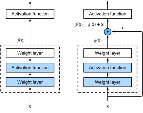
Let’s focus on a local part of a neural network, as depicted in Fig. 8.6.2. Denote the input by x. We assume that the desired underlying mapping we want to obtain by learning is f(x), to be used as input to the activation function on the top. On the left, the portion within the dotted-line box must directly learn the mapping f(x). On the right, the portion within the dotted-line box needs to learn the residual mapping g(x)=f(x)−x, which is how the residual block derives its name. If the identity mapping f(x)=x is the desired underlying mapping, the residual mapping amounts to g(x)=0 and it is thus easier to learn: we only need to push the weights and biases of the upper weight layer (e.g., fully connected layer and convolutional layer) within the dotted-line box to zero. The right figure illustrates the residual block of ResNet, where the solid line carrying the layer input x to the addition operator is called a residual connection (or shortcut connection). With residual blocks, inputs can forward propagate faster through the residual connections across layers. In fact, the residual block can be thought of as a special case of the multi-branch Inception block: it has two branches one of which is the identity mapping.
그림 8.6.2와 같이 신경망의 로컬 부분에 초점을 맞추겠습니다. x로 입력을 나타냅니다. 우리는 학습을 통해 얻고자 하는 원하는 기본 매핑이 상단의 활성화 함수에 대한 입력으로 사용되는 f(x)라고 가정합니다. 왼쪽에서 점선 상자 안의 부분은 매핑 f(x)를 직접 학습해야 합니다. 오른쪽에서 점선 상자 내의 부분은 잔차 매핑 g(x)=f(x)−x를 학습해야 하며, 이는 잔차 블록이 이름을 파생하는 방법입니다. ID 매핑 f(x)=x가 원하는 기본 매핑인 경우 잔여 매핑은 g(x)=0이 되므로 배우기가 더 쉽습니다. 상위 가중치 레이어의 가중치와 편향만 푸시하면 됩니다( 예를 들어 점선 상자 내에서 완전 연결 계층 및 컨볼루션 계층)을 0으로 설정합니다. 오른쪽 그림은 ResNet의 잔차 블록을 나타낸 것으로, 여기서 레이어 입력 x를 덧셈 연산자로 전달하는 실선을 잔차 연결(또는 바로가기 연결)이라고 합니다. 잔차 블록을 사용하면 입력이 계층 전체의 잔차 연결을 통해 더 빠르게 전달될 수 있습니다. 사실, 잔차 블록은 다중 분기 시작 블록의 특수한 경우로 생각할 수 있습니다. 여기에는 두 개의 분기가 있으며 그 중 하나는 identity mapping입니다.
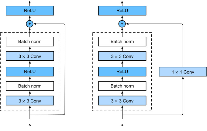
ResNet follows VGG’s full 3×3 convolutional layer design. The residual block has two 3×3 convolutional layers with the same number of output channels. Each convolutional layer is followed by a batch normalization layer and a ReLU activation function. Then, we skip these two convolution operations and add the input directly before the final ReLU activation function. This kind of design requires that the output of the two convolutional layers has to be of the same shape as the input, so that they can be added together. If we want to change the number of channels, we need to introduce an additional 1×1 convolutional layer to transform the input into the desired shape for the addition operation. Let’s have a look at the code below.
ResNet은 VGG의 전체 3×3 컨볼루션 레이어 디자인을 따릅니다. 잔차 블록에는 출력 채널 수가 같은 두 개의 3×3 컨벌루션 레이어가 있습니다. 각 컨볼루션 계층 다음에는 배치 정규화 계층과 ReLU 활성화 함수가 옵니다. 그런 다음 이 두 컨볼루션 작업을 건너뛰고 최종 ReLU 활성화 함수 바로 앞에 입력을 추가합니다. 이러한 종류의 설계에서는 두 컨볼루션 레이어의 출력이 입력과 동일한 모양이어야 하므로 함께 더할 수 있습니다. 채널 수를 변경하려면 추가 작업을 위해 입력을 원하는 모양으로 변환하기 위해 추가 1x1 컨벌루션 레이어를 도입해야 합니다. 아래 코드를 살펴보겠습니다.
class Residual(nn.Module):  #@save
    """The Residual block of ResNet models."""
    def __init__(self, num_channels, use_1x1conv=False, strides=1):
        super().__init__()
        self.conv1 = nn.LazyConv2d(num_channels, kernel_size=3, padding=1,
                                   stride=strides)
        self.conv2 = nn.LazyConv2d(num_channels, kernel_size=3, padding=1)
        if use_1x1conv:
            self.conv3 = nn.LazyConv2d(num_channels, kernel_size=1,
                                       stride=strides)
        else:
            self.conv3 = None
        self.bn1 = nn.LazyBatchNorm2d()
        self.bn2 = nn.LazyBatchNorm2d()

    def forward(self, X):
        Y = F.relu(self.bn1(self.conv1(X)))
        Y = self.bn2(self.conv2(Y))
        if self.conv3:
            X = self.conv3(X)
        Y += X
        return F.relu(Y)
위 코드는 ResNet 모델의 Residual 블록을 정의하는 클래스입니다.
- class Residual(nn.Module):: Residual 클래스는 nn.Module 클래스를 상속하여 정의됩니다. nn.Module은 PyTorch의 모델 구성 요소를 정의하기 위해 사용되는 기본 클래스입니다.
- def __init__(self, num_channels, use_1x1conv=False, strides=1):: 클래스의 생성자 함수입니다. 이 함수는 Residual 블록을 초기화하는데 필요한 파라미터들을 받습니다.
- self.conv1 = nn.LazyConv2d(num_channels, kernel_size=3, padding=1, stride=strides): 3x3 컨볼루션 레이어를 생성합니다. 이 레이어는 입력 채널의 수 num_channels로 설정되며, 커널 크기는 3x3이고 패딩은 1로 설정됩니다. strides는 컨볼루션의 보폭을 나타냅니다.
- self.conv2 = nn.LazyConv2d(num_channels, kernel_size=3, padding=1): 두 번째 3x3 컨볼루션 레이어를 생성합니다. 이 레이어의 설정은 conv1과 동일하지만, 보폭은 따로 지정하지 않아 기본 값으로 1이 됩니다.
- if use_1x1conv: ...: 만약 use_1x1conv가 True인 경우 1x1 컨볼루션 레이어를 생성합니다. 이 레이어는 입력 채널을 줄이기 위해 사용되며, 보폭은 strides와 동일하게 설정됩니다. 만약 use_1x1conv가 False라면 이 레이어는 None으로 설정됩니다.
- self.bn1 = nn.LazyBatchNorm2d(): 첫 번째 배치 정규화(Batch Normalization) 레이어를 생성합니다.
- self.bn2 = nn.LazyBatchNorm2d(): 두 번째 배치 정규화 레이어를 생성합니다.
- def forward(self, X): ...: forward 함수는 Residual 블록의 순방향 연산을 정의합니다. 입력 X를 받아서 Residual 블록을 통과시키고 결과를 반환합니다.
- Y = F.relu(self.bn1(self.conv1(X))): 입력 X를 첫 번째 컨볼루션 레이어와 배치 정규화 레이어를 통과시키고 활성화 함수 ReLU를 적용합니다.
- Y = self.bn2(self.conv2(Y)): 이후 두 번째 컨볼루션 레이어와 배치 정규화 레이어를 통과시키고 결과를 Y에 저장합니다.
- if self.conv3: X = self.conv3(X): use_1x1conv가 True일 경우 1x1 컨볼루션 레이어를 통과시키고 결과를 X에 저장합니다.
- Y += X: 이전의 Y에 이전 입력 X를 더합니다. 이것이 바로 잔차 연결(Residual Connection)을 의미합니다.
- return F.relu(Y): 최종 결과 Y를 ReLU 활성화 함수를 통과시킨 후 반환합니다.
Residual 블록은 ResNet에서 사용되는 핵심 구성 요소로, 잔차 연결을 통해 신경망의 깊이가 깊어져도 그레디언트 소실과 폭주 문제를 완화하고 더욱 쉽게 학습할 수 있도록 도와줍니다. 이 구조를 사용하면 더 깊고 더 강력한 딥러닝 모델을 구축할 수 있습니다.
This code generates two types of networks: one where we add the input to the output before applying the ReLU nonlinearity whenever use_1x1conv=False, and one where we adjust channels and resolution by means of a 1×1 convolution before adding. Fig. 8.6.3 illustrates this.
이 코드는 두 가지 유형의 네트워크를 생성합니다. 하나는 use_1x1conv=False일 때마다 ReLU 비선형성을 적용하기 전에 출력에 입력을 추가하는 것이고, 다른 하나는 추가하기 전에 1×1 컨벌루션을 통해 채널과 해상도를 조정하는 것입니다. 그림 8.6.3이 이를 설명합니다.
Now let’s look at a situation where the input and output are of the same shape, where 1×1 convolution is not needed.
이제 입력과 출력이 같은 모양으로 1×1 컨벌루션이 필요하지 않은 상황을 살펴보겠습니다.
blk = Residual(3)
X = torch.randn(4, 3, 6, 6)
blk(X).shape
위 코드는 ResNet의 Residual 블록을 정의하고, 이를 활용하여 입력 데이터 X에 대한 출력의 형태를 계산하는 예시입니다.
- blk = Residual(3): Residual 클래스를 이용하여 블록 blk를 생성합니다. 이 블록은 입력 채널이 3인 Residual 블록을 의미합니다.
- X = torch.randn(4, 3, 6, 6): 크기가 (4, 3, 6, 6)인 랜덤한 입력 데이터 X를 생성합니다. 이는 4개의 샘플, 3개의 채널, 각각 6x6 크기의 이미지로 구성된 데이터입니다.
- blk(X).shape: 생성한 blk에 입력 데이터 X를 통과시켜 출력의 형태를 계산합니다. 이 때 출력의 형태를 확인하기 위해 .shape 메서드를 사용합니다.
결과로 출력된 형태는 입력 데이터 X가 Residual 블록을 통과한 후의 결과 형태를 나타내며, (4, 3, 6, 6)입니다. 이는 입력 데이터 X와 동일한 형태를 가지고 있음을 의미합니다. Residual 블록의 역할은 입력과 출력의 차원을 보존하면서 추가적인 비선형 변환을 적용하여 딥러닝 모델의 성능을 향상시키는 것입니다.
torch.Size([4, 3, 6, 6])
We also have the option to halve the output height and width while increasing the number of output channels. In this case we use 1×1 convolutions via use_1x1conv=True. This comes in handy at the beginning of each ResNet block to reduce the spatial dimensionality via strides=2.
또한 출력 채널 수를 늘리면서 출력 높이와 너비를 절반으로 줄이는 옵션도 있습니다. 이 경우 use_1x1conv=True를 통해 1×1 컨볼루션을 사용합니다. 이것은 strides=2를 통해 공간 차원을 줄이기 위해 각 ResNet 블록의 시작 부분에서 유용합니다.
blk = Residual(6, use_1x1conv=True, strides=2)
blk(X).shape
위 코드는 ResNet의 Residual 블록을 정의하고, 이를 활용하여 입력 데이터 X에 대한 출력의 형태를 계산하는 예시입니다. 이번에는 Residual 블록에 use_1x1conv=True와 strides=2 옵션을 주어 블록을 생성합니다.
- blk = Residual(6, use_1x1conv=True, strides=2): Residual 클래스를 이용하여 블록 blk를 생성합니다. 이 블록은 입력 채널이 6인 Residual 블록을 의미합니다. use_1x1conv=True 옵션은 블록 내에서 1x1 컨볼루션 연산을 사용함을 의미하며, strides=2는 블록 내에서 2칸씩 이동하는 스트라이드를 사용함을 의미합니다.
- X = torch.randn(4, 6, 6, 6): 크기가 (4, 6, 6, 6)인 랜덤한 입력 데이터 X를 생성합니다. 이는 4개의 샘플, 6개의 채널, 각각 6x6 크기의 이미지로 구성된 데이터입니다.
- blk(X).shape: 생성한 blk에 입력 데이터 X를 통과시켜 출력의 형태를 계산합니다. 이 때 출력의 형태를 확인하기 위해 .shape 메서드를 사용합니다.
결과로 출력된 형태는 입력 데이터 X가 Residual 블록을 통과한 후의 결과 형태를 나타내며, (4, 6, 3, 3)입니다. 이는 입력 데이터 X의 채널 수는 그대로 유지되지만, 3x3 크기로 다운샘플링되었음을 의미합니다. strides=2 옵션에 의해 블록 내에서 2칸씩 이동하는 스트라이드를 사용하여 입력 데이터의 공간 해상도를 줄이고, use_1x1conv=True 옵션에 의해 1x1 컨볼루션 연산이 적용되어 채널 수는 유지되면서 공간 크기가 반으로 줄어든 것입니다. 이를 통해 더 깊고 복잡한 모델을 구성할 때 공간 크기를 효과적으로 줄여 계산 비용을 절감하고 성능을 향상시킬 수 있습니다.
torch.Size([4, 6, 3, 3])
8.6.3. ResNet Model
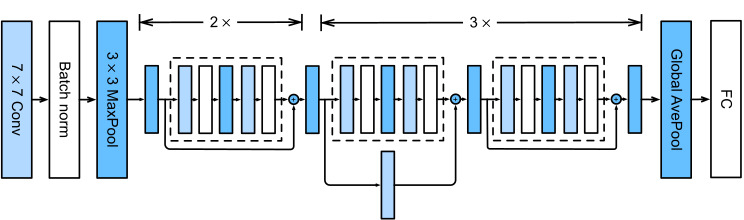
The first two layers of ResNet are the same as those of the GoogLeNet we described before: the 7×7 convolutional layer with 64 output channels and a stride of 2 is followed by the 3×3 max-pooling layer with a stride of 2. The difference is the batch normalization layer added after each convolutional layer in ResNet.
ResNet의 처음 두 레이어는 이전에 설명한 GoogLeNet의 레이어와 동일합니다. 출력 채널이 64개이고 스트라이드가 2인 7×7 컨볼루션 레이어 다음에는 스트라이드가 2인 3×3 최대 풀링 레이어가 있습니다. 차이점은 ResNet의 각 컨볼루션 계층 뒤에 배치 정규화 계층이 추가된다는 것입니다.
class ResNet(d2l.Classifier):
    def b1(self):
        return nn.Sequential(
            nn.LazyConv2d(64, kernel_size=7, stride=2, padding=3),
            nn.LazyBatchNorm2d(), nn.ReLU(),
            nn.MaxPool2d(kernel_size=3, stride=2, padding=1))
위 코드는 ResNet의 블록을 정의하는 클래스 ResNet입니다. 이 클래스는 d2l.Classifier를 상속하여 정의되었습니다. 해당 클래스 내의 b1 함수는 ResNet에서 첫 번째 블록을 의미합니다. 이 블록은 입력 이미지의 크기를 줄이기 위한 역할을 합니다.
- nn.Sequential: nn.Sequential을 사용하여 여러 레이어를 차례대로 쌓아 순차적으로 실행하는 블록을 생성합니다.
- nn.LazyConv2d(64, kernel_size=7, stride=2, padding=3): 입력 채널 수가 64인 2D 컨볼루션 레이어를 생성합니다. 커널 크기는 7x7이며, 스트라이드는 2로 설정되어 입력 이미지의 공간 해상도를 절반으로 줄입니다. 패딩은 3으로 설정되어 입력 이미지의 크기를 유지합니다.
- nn.LazyBatchNorm2d(): 배치 정규화(Batch Normalization) 레이어를 생성합니다. 배치 정규화는 학습을 안정화시키고 더 빠른 수렴을 도와주는 기법으로, 블록 내의 각 채널에 대해 평균과 표준 편차를 구해 정규화를 수행합니다.
- nn.ReLU(): ReLU(ReLU, Rectified Linear Unit) 활성화 함수를 적용합니다. ReLU는 입력값이 양수일 경우 그대로 출력하고, 음수일 경우 0으로 출력합니다.
- nn.MaxPool2d(kernel_size=3, stride=2, padding=1): 2D 최대 풀링 레이어를 생성합니다. 커널 크기는 3x3이며, 스트라이드는 2로 설정되어 입력 이미지의 공간 해상도를 절반으로 줄입니다. 패딩은 1로 설정되어 입력 이미지의 크기를 유지합니다.
이렇게 정의된 b1 함수는 ResNet의 첫 번째 블록으로, 입력 이미지의 공간 해상도를 절반으로 줄이고, 일부 채널에 배치 정규화와 ReLU 활성화 함수를 적용하는 과정을 담고 있습니다.
GoogLeNet uses four modules made up of Inception blocks. However, ResNet uses four modules made up of residual blocks, each of which uses several residual blocks with the same number of output channels. The number of channels in the first module is the same as the number of input channels. Since a max-pooling layer with a stride of 2 has already been used, it is not necessary to reduce the height and width. In the first residual block for each of the subsequent modules, the number of channels is doubled compared with that of the previous module, and the height and width are halved.
GoogLeNet은 Inception 블록으로 구성된 4개의 모듈을 사용합니다. 그러나 ResNet은 잔차 블록으로 구성된 4개의 모듈을 사용하며, 각 모듈은 동일한 수의 출력 채널을 가진 여러 잔차 블록을 사용합니다. 첫 번째 모듈의 채널 수는 입력 채널 수와 동일합니다. stride가 2인 max-pooling 레이어가 이미 사용되었으므로 높이와 너비를 줄일 필요가 없습니다. 각 후속 모듈에 대한 첫 번째 잔차 블록에서 채널 수는 이전 모듈에 비해 두 배가 되고 높이와 너비는 절반으로 줄어듭니다.
@d2l.add_to_class(ResNet)
def block(self, num_residuals, num_channels, first_block=False):
    blk = []
    for i in range(num_residuals):
        if i == 0 and not first_block:
            blk.append(Residual(num_channels, use_1x1conv=True, strides=2))
        else:
            blk.append(Residual(num_channels))
    return nn.Sequential(*blk)
위 코드는 ResNet 클래스에 새로운 함수인 block을 추가하는 부분입니다.
- @d2l.add_to_class(ResNet): 이 부분은 ResNet 클래스에 새로운 함수를 추가하기 위해 데코레이터를 사용하는 부분입니다.
- def block(self, num_residuals, num_channels, first_block=False):: block 함수는 ResNet의 블록을 구성하는 함수입니다. 이 함수는 다음과 같은 인자를 받습니다.
- num_residuals: 각 블록에 포함되는 Residual 레이어의 개수입니다.
- num_channels: Residual 레이어의 출력 채널 수입니다.
- first_block: 첫 번째 블록인지 여부를 나타내는 불리언 값입니다. 기본값은 False이며, 첫 번째 블록이 아님을 의미합니다.
- blk = []: 빈 리스트를 생성하여 블록을 담을 리스트를 초기화합니다.
- for i in range(num_residuals):: 지정된 num_residuals 만큼 반복문을 수행합니다.
- if i == 0 and not first_block:: 첫 번째 Residual 레이어가 아니고 첫 번째 블록인 경우를 확인합니다.
- blk.append(Residual(num_channels, use_1x1conv=True, strides=2)): 첫 번째 Residual 레이어이며 1x1 컨볼루션 레이어를 사용하고 스트라이드를 2로 설정하여 입력 이미지의 공간 해상도를 절반으로 줄입니다.
- else:
- blk.append(Residual(num_channels)): 나머지 경우에는 일반적인 Residual 레이어를 추가합니다.
- return nn.Sequential(*blk): 생성된 블록 리스트를 nn.Sequential로 묶어서 순차적으로 실행되도록 만듭니다.
이렇게 정의된 block 함수는 ResNet에서 여러 개의 Residual 레이어로 구성된 블록을 만드는 역할을 합니다. 첫 번째 블록인 경우에는 1x1 컨볼루션 레이어와 스트라이드를 사용하여 입력 이미지의 공간 해상도를 절반으로 줄이고, 그 외에는 일반적인 Residual 레이어를 반복하여 쌓습니다. 이렇게 생성된 블록은 순차적으로 연결되어 ResNet의 핵심적인 구조를 형성합니다.
Then, we add all the modules to ResNet. Here, two residual blocks are used for each module. Lastly, just like GoogLeNet, we add a global average pooling layer, followed by the fully connected layer output.
그런 다음 모든 모듈을 ResNet에 추가합니다. 여기서 각 모듈에 대해 두 개의 잔차 블록이 사용됩니다. 마지막으로 GoogLeNet과 마찬가지로 전역 평균 풀링 레이어를 추가한 다음 완전히 연결된 레이어 출력을 추가합니다.
@d2l.add_to_class(ResNet)
def __init__(self, arch, lr=0.1, num_classes=10):
    super(ResNet, self).__init__()
    self.save_hyperparameters()
    self.net = nn.Sequential(self.b1())
    for i, b in enumerate(arch):
        self.net.add_module(f'b{i+2}', self.block(*b, first_block=(i==0)))
    self.net.add_module('last', nn.Sequential(
        nn.AdaptiveAvgPool2d((1, 1)), nn.Flatten(),
        nn.LazyLinear(num_classes)))
    self.net.apply(d2l.init_cnn)
위 코드는 ResNet 클래스의 생성자 __init__에 새로운 기능을 추가하는 부분입니다.
- @d2l.add_to_class(ResNet): 이 부분은 ResNet 클래스에 새로운 함수를 추가하기 위해 데코레이터를 사용하는 부분입니다.
- def __init__(self, arch, lr=0.1, num_classes=10):: __init__ 함수는 ResNet의 생성자입니다. 이 함수는 다음과 같은 인자를 받습니다.
- arch: 블록들의 구조를 정의한 튜플들의 리스트입니다. 각 튜플은 다음과 같은 정보를 포함합니다.
- num_residuals: 각 블록에 포함되는 Residual 레이어의 개수입니다.
- num_channels: Residual 레이어의 출력 채널 수입니다.
- lr: 학습률을 나타내는 값입니다. 기본값은 0.1입니다.
- num_classes: 분류할 클래스의 개수입니다. 기본값은 10입니다.
- arch: 블록들의 구조를 정의한 튜플들의 리스트입니다. 각 튜플은 다음과 같은 정보를 포함합니다.
- super(ResNet, self).__init__(): 상위 클래스인 ResNet의 생성자를 호출하여 초기화합니다.
- self.save_hyperparameters(): 하이퍼파라미터들을 저장합니다.
- self.net = nn.Sequential(self.b1()): ResNet의 첫 번째 블록인 b1을 순차적으로 실행할 수 있도록 nn.Sequential로 초기화합니다.
- for i, b in enumerate(arch):: arch에서 각 블록의 정보를 가져옵니다. enumerate 함수를 사용하여 인덱스와 함께 반복합니다.
- self.net.add_module(f'b{i+2}', self.block(*b, first_block=(i==0))): i+2와 b를 사용하여 블록을 순차적으로 추가합니다. first_block 인자는 첫 번째 블록인 경우에 True로 설정하여 1x1 컨볼루션 레이어와 스트라이드를 사용하도록 합니다.
- self.net.add_module('last', nn.Sequential(: 마지막 블록인 last를 추가합니다.
- nn.AdaptiveAvgPool2d((1, 1)): 주어진 입력 크기에 따라 적응적 평균 풀링 레이어를 생성합니다. 입력 크기를 (1, 1)로 설정하여 공간 차원을 평균화합니다.
- nn.Flatten(): 다차원 텐서를 일차원으로 평면화하는 레이어입니다.
- nn.LazyLinear(num_classes)): num_classes를 출력 크기로 하는 선형 레이어를 생성합니다.
- self.net.apply(d2l.init_cnn): 생성된 ResNet 모델에 CNN 레이어들을 초기화하는 함수인 d2l.init_cnn을 적용합니다.
이렇게 정의된 ResNet 클래스는 입력으로 받은 arch에 따라서 여러 개의 ResNet 블록들을 순차적으로 추가하여 ResNet 모델을 만들게 됩니다. 이때, 첫 번째 블록은 1x1 컨볼루션 레이어와 스트라이드를 사용하여 입력 이미지의 공간 해상도를 줄이게 됩니다. 그리고 마지막 블록에는 평균 풀링과 선형 레이어를 추가하여 최종적으로 출력 클래스의 개수에 맞는 예측 결과를 얻습니다. 이렇게 구성된 ResNet 모델은 self.net에 저장되어 있으며 학습 및 추론에 사용할 수 있습니다.
There are 4 convolutional layers in each module (excluding the 1×1 convolutional layer). Together with the first 7×7 convolutional layer and the final fully connected layer, there are 18 layers in total. Therefore, this model is commonly known as ResNet-18. By configuring different numbers of channels and residual blocks in the module, we can create different ResNet models, such as the deeper 152-layer ResNet-152. Although the main architecture of ResNet is similar to that of GoogLeNet, ResNet’s structure is simpler and easier to modify. All these factors have resulted in the rapid and widespread use of ResNet. Fig. 8.6.4 depicts the full ResNet-18.
각 모듈에는 4개의 컨볼루션 레이어가 있습니다(1×1 컨볼루션 레이어 제외). 첫 번째 7×7 컨볼루션 레이어와 마지막 완전 연결 레이어를 포함하여 총 18개의 레이어가 있습니다. 따라서 이 모델은 일반적으로 ResNet-18로 알려져 있습니다. 모듈에서 서로 다른 수의 채널과 잔차 블록을 구성하여 더 깊은 152계층 ResNet-152와 같은 다양한 ResNet 모델을 생성할 수 있습니다. ResNet의 주요 아키텍처는 GoogLeNet과 유사하지만 ResNet의 구조는 더 간단하고 수정하기 쉽습니다. 이러한 모든 요인으로 인해 ResNet이 빠르고 광범위하게 사용되었습니다. 그림 8.6.4는 전체 ResNet-18을 보여줍니다.
Before training ResNet, let’s observe how the input shape changes across different modules in ResNet. As in all the previous architectures, the resolution decreases while the number of channels increases up until the point where a global average pooling layer aggregates all features.
ResNet을 교육하기 전에 ResNet의 여러 모듈에서 입력 모양이 어떻게 변경되는지 살펴보겠습니다. 이전의 모든 아키텍처와 마찬가지로 전역 평균 풀링 레이어가 모든 기능을 집계하는 지점까지 채널 수가 증가하는 동안 해상도는 감소합니다.
class ResNet18(ResNet):
    def __init__(self, lr=0.1, num_classes=10):
        super().__init__(((2, 64), (2, 128), (2, 256), (2, 512)),
                       lr, num_classes)

ResNet18().layer_summary((1, 1, 96, 96))
위 코드는 ResNet18 모델을 정의하는 부분과 해당 모델의 레이어 구성을 확인하는 코드로 이루어져 있습니다.
- class ResNet18(ResNet): ResNet18 클래스는 ResNet 클래스를 상속받습니다. 따라서 ResNet18 클래스는 ResNet 클래스의 모든 기능과 구조를 상속받아 사용할 수 있습니다.
- def __init__(self, lr=0.1, num_classes=10): ResNet18의 생성자 함수입니다. 이 함수는 다음과 같은 인자를 받습니다.
- lr: 학습률을 나타내는 값으로 기본값은 0.1입니다.
- num_classes: 분류할 클래스의 개수로 기본값은 10입니다.
- super().__init__(((2, 64), (2, 128), (2, 256), (2, 512)), lr, num_classes): ResNet 클래스의 생성자를 호출하여 ResNet18 모델을 초기화합니다. 인자로는 ResNet18 모델의 구조를 정의하는 튜플들의 리스트를 전달합니다. 각 튜플은 다음과 같은 정보를 포함합니다.
- num_residuals: 각 Residual 블록에 포함되는 레이어의 개수입니다.
- num_channels: Residual 블록의 출력 채널 수입니다.
- ResNet18().layer_summary((1, 1, 96, 96)): ResNet18 모델의 레이어 구성을 확인하는 코드입니다. 이를 위해 layer_summary 함수를 사용하여 입력 이미지 크기가 (1, 1, 96, 96)인 경우의 모델 구성을 요약해서 보여줍니다.
ResNet18 모델은 ResNet 클래스를 상속받아 ResNet 구조에 기반하여 만들어졌으며, ResNet18 모델의 구조는 18개의 레이어를 가진 ResNet 버전입니다. 또한 layer_summary 함수를 사용하여 모델의 레이어 구성을 확인할 수 있습니다.
Sequential output shape:     torch.Size([1, 64, 24, 24])
Sequential output shape:     torch.Size([1, 64, 24, 24])
Sequential output shape:     torch.Size([1, 128, 12, 12])
Sequential output shape:     torch.Size([1, 256, 6, 6])
Sequential output shape:     torch.Size([1, 512, 3, 3])
Sequential output shape:     torch.Size([1, 10])
8.6.4. Training
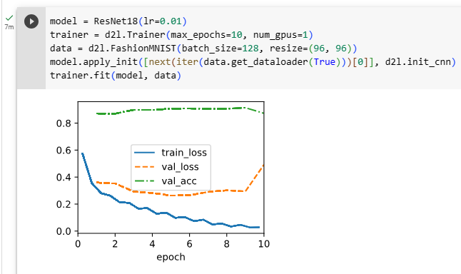
We train ResNet on the Fashion-MNIST dataset, just like before. ResNet is quite a powerful and flexible architecture. The plot capturing training and validation loss illustrates a significant gap between both graphs, with the training loss being significantly lower. For a network of this flexibility, more training data would offer significant benefit in closing the gap and improving accuracy.
이전과 마찬가지로 Fashion-MNIST 데이터 세트에서 ResNet을 교육합니다. ResNet은 매우 강력하고 유연한 아키텍처입니다. 훈련 및 검증 손실을 캡처하는 플롯은 훈련 손실이 훨씬 더 낮은 두 그래프 사이의 상당한 차이를 보여줍니다. 이러한 유연성을 갖춘 네트워크의 경우 더 많은 교육 데이터가 격차를 좁히고 정확도를 개선하는 데 상당한 이점을 제공할 것입니다.
model = ResNet18(lr=0.01)
trainer = d2l.Trainer(max_epochs=10, num_gpus=1)
data = d2l.FashionMNIST(batch_size=128, resize=(96, 96))
model.apply_init([next(iter(data.get_dataloader(True)))[0]], d2l.init_cnn)
trainer.fit(model, data)
위 코드는 ResNet18 모델을 생성하고 이를 FashionMNIST 데이터셋으로 학습하는 과정을 나타내고 있습니다.
- model = ResNet18(lr=0.01): ResNet18 모델을 생성하고 학습률을 0.01로 설정하여 초기화합니다.
- trainer = d2l.Trainer(max_epochs=10, num_gpus=1): d2l 라이브러리의 Trainer를 생성합니다. 이 때, 최대 에폭(epoch)을 10으로 설정하고 하나의 GPU를 사용하여 학습합니다.
- data = d2l.FashionMNIST(batch_size=128, resize=(96, 96)): FashionMNIST 데이터셋을 생성합니다. 이 데이터셋은 배치 크기를 128로 설정하고 이미지 크기를 (96, 96)으로 변환합니다.
- model.apply_init([next(iter(data.get_dataloader(True)))[0]], d2l.init_cnn): 모델의 가중치를 초기화합니다. 이를 위해 FashionMNIST 데이터셋의 첫 번째 배치를 가져와서 모델에 적용하여 가중치를 초기화합니다. 초기화 방법으로는 d2l.init_cnn 함수를 사용합니다.
- trainer.fit(model, data): 생성한 모델과 데이터셋을 사용하여 학습을 수행합니다. Trainer의 fit 함수를 호출하여 모델을 학습시키고, 데이터셋을 사용하여 모델을 평가합니다. 학습은 최대 10 에폭까지 진행됩니다.
이 코드는 ResNet18 모델을 FashionMNIST 데이터셋으로 학습하는 과정을 단계별로 나타낸 것입니다. ResNet18 모델을 생성하고 학습 데이터셋으로 학습하여 모델을 최적화하는 과정을 쉽게 이해할 수 있도록 코드로 표현한 것입니다.

8.6.5. ResNeXt
One of the challenges one encounters in the design of ResNet is the trade-off between nonlinearity and dimensionality within a given block. That is, we could add more nonlinearity by increasing the number of layers, or by increasing the width of the convolutions. An alternative strategy is to increase the number of channels that can carry information between blocks. Unfortunately, the latter comes with a quadratic penalty since the computational cost of ingesting ci channels and emitting co channels is proportional to O(ci⋅co) (see our discussion in Section 7.4).
ResNet 설계에서 직면하는 문제 중 하나는 주어진 블록 내에서 비선형성과 차원 간의 절충입니다. 즉, 레이어 수를 늘리거나 컨볼루션의 너비를 늘려 더 많은 비선형성을 추가할 수 있습니다. 대안 전략은 블록 간에 정보를 전달할 수 있는 채널의 수를 늘리는 것입니다. 불행하게도 후자는 ci 채널을 수집하고 co 채널을 방출하는 계산 비용이 O(ci⋅co)에 비례하기 때문에 2차 페널티가 있습니다(섹션 7.4의 논의 참조).
We can take some inspiration from the Inception block of Fig. 8.4.1 which has information flowing through the block in separate groups. Applying the idea of multiple independent groups to the ResNet block of Fig. 8.6.3 led to the design of ResNeXt (Xie et al., 2017). Different from the smorgasbord of transformations in Inception, ResNeXt adopts the same transformation in all branches, thus minimizing the need for manual tuning of each branch.
그림 8.4.1의 인셉션 블록에서 정보가 개별 그룹으로 흐르는 정보를 가지고 있는 것에서 영감을 얻을 수 있습니다. 그림 8.6.3의 ResNet 블록에 여러 독립 그룹의 아이디어를 적용하면 ResNeXt가 설계되었습니다(Xie et al., 2017). Inception의 다양한 변환과 달리 ResNeXt는 모든 분기에서 동일한 변환을 채택하므로 각 분기의 수동 조정 필요성이 최소화됩니다.
Breaking up a convolution from ci to co channels into one of g groups of size ci/g generating g outputs of size co/g is called, quite fittingly, a grouped convolution. The computational cost (proportionally) is reduced from O(ci⋅co) to O(g⋅(ci/g)⋅(co/g))=O(ci⋅co/g), i.e., it is g times faster. Even better, the number of parameters needed to generate the output is also reduced from a ci×co matrix to g smaller matrices of size (ci/g)×(co/g), again a g times reduction. In what follows we assume that both ci and co are divisible by g.
ci에서 co 채널로의 컨볼루션을 크기 co/g의 g 출력을 생성하는 크기 ci/g의 g 그룹 중 하나로 분해하는 것을 그룹화 컨벌루션이라고 합니다. 계산 비용은 (비례적으로) O(ci⋅co)에서 O(g⋅(ci/g)⋅(co/g))=O(ci⋅co/g)로 감소합니다. 즉, g배 더 빠릅니다. 더 좋은 점은 출력을 생성하는 데 필요한 매개변수의 수도 ci×co 행렬에서 (ci/g)×(co/g) 크기의 더 작은 행렬 g로 줄어 다시 g배 감소한다는 것입니다. 다음에서 우리는 ci와 co 모두 g로 나눌 수 있다고 가정합니다.
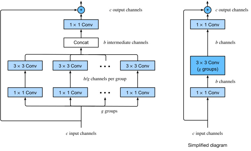
The only challenge in this design is that no information is exchanged between the g groups. The ResNeXt block of Fig. 8.6.5 amends this in two ways: the grouped convolution with a 3×3 kernel is sandwiched in between two 1×1 convolutions. The second one serves double duty in changing the number of channels back. The benefit is that we only pay the O(c⋅b) cost for 1×1 kernels and can make do with an O(b2/g) cost for 3×3 kernels. Similar to the residual block implementation in Section 8.6.2, the residual connection is replaced (thus generalized) by a 1×1 convolution.
이 디자인의 유일한 문제는 g 그룹 간에 정보가 교환되지 않는다는 것입니다. 그림 8.6.5의 ResNeXt 블록은 이를 두 가지 방식으로 수정합니다. 3×3 커널이 있는 그룹화된 컨볼루션이 두 개의 1×1 컨볼루션 사이에 끼어 있습니다. 두 번째는 채널 수를 다시 변경하는 이중 역할을 합니다. 이점은 1×1 커널에 대한 O(c⋅b) 비용만 지불하고 3×3 커널에 대한 O(b2/g) 비용으로 해결할 수 있다는 것입니다. 섹션 8.6.2의 잔차 블록 구현과 유사하게 잔차 연결은 1×1 컨벌루션으로 대체됩니다(따라서 일반화됨).
The right figure in Fig. 8.6.5 provides a much more concise summary of the resulting network block. It will also play a major role in the design of generic modern CNNs in Section 8.8. Note that the idea of grouped convolutions dates back to the implementation of AlexNet (Krizhevsky et al., 2012). When distributing the network across two GPUs with limited memory, the implementation treated each GPU as its own channel with no ill effects.
그림 8.6.5의 오른쪽 그림은 결과 네트워크 블록에 대한 훨씬 더 간결한 요약을 제공합니다. 또한 섹션 8.8에서 일반적인 최신 CNN 설계에 중요한 역할을 할 것입니다. 그룹 컨볼루션의 아이디어는 AlexNet 구현으로 거슬러 올라갑니다(Krizhevsky et al., 2012). 메모리가 제한된 두 개의 GPU에 네트워크를 분산할 때 구현 시 각 GPU를 악영향 없이 자체 채널로 처리했습니다.
The following implementation of the ResNeXtBlock class takes as argument groups (g), with bot_channels (b) intermediate (bottleneck) channels. Lastly, when we need to reduce the height and width of the representation, we add a stride of 2 by setting use_1x1conv=True, strides=2.
ResNeXtBlock 클래스의 다음 구현은 인수 그룹(g)과 bot_channels(b) 중간(병목) 채널을 사용합니다. 마지막으로 표현의 높이와 너비를 줄여야 할 때 use_1x1conv=True, strides=2를 설정하여 stride 2를 추가합니다.
class ResNeXtBlock(nn.Module):  #@save
    """The ResNeXt block."""
    def __init__(self, num_channels, groups, bot_mul, use_1x1conv=False,
                 strides=1):
        super().__init__()
        bot_channels = int(round(num_channels * bot_mul))
        self.conv1 = nn.LazyConv2d(bot_channels, kernel_size=1, stride=1)
        self.conv2 = nn.LazyConv2d(bot_channels, kernel_size=3,
                                   stride=strides, padding=1,
                                   groups=bot_channels//groups)
        self.conv3 = nn.LazyConv2d(num_channels, kernel_size=1, stride=1)
        self.bn1 = nn.LazyBatchNorm2d()
        self.bn2 = nn.LazyBatchNorm2d()
        self.bn3 = nn.LazyBatchNorm2d()
        if use_1x1conv:
            self.conv4 = nn.LazyConv2d(num_channels, kernel_size=1,
                                       stride=strides)
            self.bn4 = nn.LazyBatchNorm2d()
        else:
            self.conv4 = None

    def forward(self, X):
        Y = F.relu(self.bn1(self.conv1(X)))
        Y = F.relu(self.bn2(self.conv2(Y)))
        Y = self.bn3(self.conv3(Y))
        if self.conv4:
            X = self.bn4(self.conv4(X))
        return F.relu(Y + X)
위 코드는 ResNeXt 블록을 정의한 클래스인 ResNeXtBlock을 나타내고 있습니다.
ResNeXt 블록은 ResNet과 유사한 구조를 가지며, 여러 그룹으로 나누어 병렬적으로 처리하는 특징을 가지고 있습니다. 각각의 그룹은 동일한 작은 네트워크 블록을 가지고 있으며, 이들을 병렬적으로 실행함으로써 더 강력한 표현력을 얻을 수 있습니다.
ResNeXtBlock 클래스는 다음과 같은 인자들을 사용하여 초기화됩니다.
- num_channels: 블록의 입력 채널 수입니다.
- groups: 그룹 수입니다. 그룹의 수가 채널의 수를 나눈 값이며, 각 그룹은 병렬적으로 작동합니다.
- bot_mul: 작은 네트워크 블록의 채널 수를 조절하는 비율입니다.
- use_1x1conv: 1x1 합성곱을 사용할지 여부를 결정하는 플래그입니다.
- strides: 컨볼루션 연산의 스트라이드 값을 지정합니다.
ResNeXtBlock 클래스는 다음과 같은 레이어들을 가지고 있습니다.
- self.conv1: 1x1 컨볼루션 레이어
- self.conv2: 3x3 컨볼루션 레이어
- self.conv3: 1x1 컨볼루션 레이어
- self.bn1, self.bn2, self.bn3: 배치 정규화(Batch Normalization) 레이어들
- self.conv4, self.bn4: use_1x1conv가 True일 경우 추가로 사용되는 1x1 컨볼루션 레이어와 배치 정규화 레이어
forward 함수는 블록의 순전파(forward) 연산을 정의하고 있습니다. 입력 X를 먼저 1x1 컨볼루션 레이어를 통과시킨 후 배치 정규화와 ReLU 활성화 함수를 적용합니다. 다음으로 3x3 컨볼루션 레이어를 통과시킨 후 다시 배치 정규화와 ReLU를 적용합니다. 그리고 다시 1x1 컨볼루션 레이어와 배치 정규화를 거친 후 추가적으로 self.conv4와 self.bn4를 사용하는 경우 해당 레이어를 통과시킵니다. 최종적으로 ReLU를 적용한 후 입력 X와 더해진 결과를 반환합니다. 이를 통해 ResNeXt 블록의 순전파 연산이 수행됩니다.
Its use is entirely analogous to that of the ResNetBlock discussed previously. For instance, when using (use_1x1conv=False, strides=1), the input and output are of the same shape. Alternatively, setting use_1x1conv=True, strides=2 halves the output height and width.
그 사용은 이전에 논의된 ResNetBlock의 사용과 완전히 유사합니다. 예를 들어 (use_1x1conv=False, strides=1)을 사용하면 입력과 출력이 같은 모양입니다. 또는 use_1x1conv=True, strides=2로 설정하면 출력 높이와 너비가 반으로 줄어듭니다.
blk = ResNeXtBlock(32, 16, 1)
X = torch.randn(4, 32, 96, 96)
blk(X).shape
위 코드는 ResNeXt 블록인 ResNeXtBlock 클래스를 사용하여 새로운 블록 blk를 생성하고, 임의의 입력 데이터 X에 대해 blk를 통과시킨 후 출력의 크기를 확인하는 내용입니다.
ResNeXtBlock은 다음과 같은 인자들을 사용하여 초기화됩니다.
- num_channels: 블록의 입력 채널 수입니다. 위 코드에서는 32로 설정되어 있습니다.
- groups: 그룹 수입니다. 그룹의 수가 채널의 수를 나눈 값이며, 각 그룹은 병렬적으로 작동합니다. 위 코드에서는 16으로 설정되어 있습니다.
- bot_mul: 작은 네트워크 블록의 채널 수를 조절하는 비율입니다. 위 코드에서는 1로 설정되어 있습니다.
- use_1x1conv: 1x1 합성곱을 사용할지 여부를 결정하는 플래그입니다. 위 코드에서는 False로 설정되어 있으므로 1x1 합성곱은 사용되지 않습니다.
- strides: 컨볼루션 연산의 스트라이드 값을 지정합니다. 위 코드에서는 기본값인 1로 설정되어 있습니다.
위 코드에서는 ResNeXtBlock을 사용하여 blk 객체를 생성한 후, 크기가 (4, 32, 96, 96)인 입력 데이터 X를 blk에 통과시키고, 최종적으로 출력의 크기를 확인하는 작업을 수행합니다.
출력의 크기를 확인하기 위해 blk(X).shape를 호출하면, 입력 X를 blk에 통과시켜 나온 출력의 크기를 반환합니다. 위 코드에서는 입력 X의 크기가 (4, 32, 96, 96)이므로 blk(X)의 출력 크기 또한 (4, 32, 96, 96)입니다. 이 결과는 ResNeXt 블록의 순전파 연산을 통해 출력이 입력과 동일한 크기를 가지는 것을 의미합니다.
torch.Size([4, 32, 96, 96])
8.6.6. Summary and Discussion
Nested function classes are desirable since they allow us to obtain strictly more powerful rather than also subtly different function classes when adding capacity. One way to accomplish this is by allowing additional layers to simply pass through the input to the output. Residual connections allow for this. As a consequence, this changes the inductive bias from simple functions being of the form f(x)=0 to simple functions looking like f(x)=x.
중첩된 함수 클래스는 용량을 추가할 때 미묘하게 다른 함수 클래스가 아니라 엄격하게 더 강력한 기능을 얻을 수 있기 때문에 바람직합니다. 이를 달성하는 한 가지 방법은 추가 레이어가 단순히 입력을 통해 출력으로 전달되도록 하는 것입니다. 잔여 연결이 이를 허용합니다. 결과적으로 이것은 f(x)=0 형식의 단순 함수에서 f(x)=x처럼 보이는 단순 함수로 유도 편향을 변경합니다.
The residual mapping can learn the identity function more easily, such as pushing parameters in the weight layer to zero. We can train an effective deep neural network by having residual blocks. Inputs can forward propagate faster through the residual connections across layers. As a consequence, we can thus train much deeper networks. For instance, the original ResNet paper (He et al., 2016) allowed for up to 152 layers. Another benefit of residual networks is that it allows us to add layers, initialized as the identity function, during the training process. After all, the default behavior of a layer is to let the data pass through unchanged. This can accelerate the training of very large networks in some cases.
residual 매핑은 가중치 계층의 매개변수를 0으로 푸는 것과 같이 항등 함수를 보다 쉽게 학습할 수 있습니다. 잔차 블록을 가짐으로써 효과적인 심층 신경망을 훈련시킬 수 있습니다. 입력은 레이어 전체의 나머지 연결을 통해 더 빠르게 전달될 수 있습니다. 결과적으로 우리는 훨씬 더 깊은 네트워크를 훈련시킬 수 있습니다. 예를 들어 원래 ResNet 논문(He et al., 2016)은 최대 152개의 레이어를 허용했습니다. 잔여 네트워크의 또 다른 이점은 훈련 과정 중에 항등 함수로 초기화된 계층을 추가할 수 있다는 것입니다. 결국 레이어의 기본 동작은 데이터가 변경되지 않은 상태로 전달되도록 하는 것입니다. 이것은 경우에 따라 매우 큰 네트워크의 훈련을 가속화할 수 있습니다.
Prior to residual connections, bypassing paths with gating units were introduced to effectively train highway networks with over 100 layers (Srivastava et al., 2015). Using identity functions as bypassing paths, ResNet performed remarkably well on multiple computer vision tasks. Residual connections had a major influence on the design of subsequent deep neural networks, both for convolutional and sequential nature. As we will introduce later, the Transformer architecture (Vaswani et al., 2017) adopts residual connections (together with other design choices) and is pervasive in areas as diverse as language, vision, speech, and reinforcement learning.
잔류 연결 이전에는 게이팅 장치가 있는 우회 경로가 도입되어 100개 이상의 레이어가 있는 고속도로 네트워크를 효과적으로 훈련했습니다(Srivastava et al., 2015). ID 기능을 우회 경로로 사용하여 ResNet은 여러 컴퓨터 비전 작업에서 놀라운 성능을 보였습니다. 잔여 연결은 컨볼루션 및 순차 특성 모두에 대해 후속 심층 신경망 설계에 큰 영향을 미쳤습니다. 나중에 소개하겠지만 Transformer 아키텍처(Vaswani et al., 2017)는 잔류 연결(다른 설계 선택과 함께)을 채택하고 언어, 시각, 음성 및 강화 학습과 같은 다양한 영역에 널리 퍼져 있습니다.
ResNeXt is an example for how the design of convolutional neural networks has evolved over time: by being more frugal with computation and trading it off with the size of the activations (number of channels), it allows for faster and more accurate networks at lower cost. An alternative way of viewing grouped convolutions is to think of a block-diagonal matrix for the convolutional weights. Note that there are quite a few such “tricks” that lead to more efficient networks. For instance, ShiftNet (Wu et al., 2018) mimicks the effects of a 3×3 convolution, simply by adding shifted activations to the channels, offering increased function complexity, this time without any computational cost.
ResNeXt는 컨볼루션 신경망의 설계가 시간이 지남에 따라 어떻게 발전해 왔는지에 대한 예입니다. 계산을 더 검소하게 하고 활성화 크기(채널 수)와 교환함으로써 더 낮은 비용으로 더 빠르고 더 정확한 네트워크를 허용합니다. . 그룹화된 컨볼루션을 보는 또 다른 방법은 컨볼루션 가중치에 대한 블록-대각선 행렬을 생각하는 것입니다. 보다 효율적인 네트워크로 이끄는 이러한 "트릭"이 상당히 많이 있다는 점에 유의하십시오. 예를 들어, ShiftNet(Wu et al., 2018)은 단순히 채널에 이동된 활성화를 추가하여 3×3 컨볼루션의 효과를 모방하여 이번에는 계산 비용 없이 향상된 기능 복잡성을 제공합니다.
A common feature of the designs we have discussed so far is that the network design is fairly manual, primarily relying on the ingenuity of the designer to find the “right” network hyperparameters. While clearly feasible, it is also very costly in terms of human time and there is no guarantee that the outcome is optimal in any sense. In Section 8.8 we will discuss a number of strategies for obtaining high quality networks in a more automated fashion. In particular, we will review the notion of network design spaces that led to the RegNetX/Y models (Radosavovic et al., 2020).
지금까지 논의한 설계의 공통적인 특징은 네트워크 설계가 "올바른" 네트워크 하이퍼파라미터를 찾기 위해 디자이너의 독창성에 주로 의존하는 상당히 수동적이라는 것입니다. 분명히 실현 가능하지만 인적 시간 측면에서 비용이 많이 들고 결과가 어떤 의미에서든 최적이라는 보장이 없습니다. 섹션 8.8에서 우리는 보다 자동화된 방식으로 고품질 네트워크를 얻기 위한 여러 가지 전략에 대해 논의할 것입니다. 특히, RegNetX/Y 모델(Radosavovic et al., 2020)로 이어진 네트워크 설계 공간의 개념을 검토할 것입니다.
8.6.7. Exercises
- What are the major differences between the Inception block in Fig. 8.4.1 and the residual block? How do they compare in terms of computation, accuracy, and the classes of functions they can describe?
- Refer to Table 1 in the ResNet paper (He et al., 2016) to implement different variants of the network.
- For deeper networks, ResNet introduces a “bottleneck” architecture to reduce model complexity. Try to implement it.
- In subsequent versions of ResNet, the authors changed the “convolution, batch normalization, and activation” structure to the “batch normalization, activation, and convolution” structure. Make this improvement yourself. See Figure 1 in He et al. (2016) for details.
- Why can’t we just increase the complexity of functions without bound, even if the function classes are nested?
'Dive into Deep Learning > D2L Convolutional Neural Networks (CNN)' 카테고리의 다른 글
| D2L - 8.8. Designing Convolution Network Architectures (0) | 2023.07.18 |
|---|---|
| D2L - 8.7. Densely Connected Networks (DenseNet) (0) | 2023.07.18 |
| D2L - 8.5. Batch Normalization (0) | 2023.07.18 |
| D2L - 8.4. Multi-Branch Networks (GoogLeNet) (0) | 2023.07.18 |
| D2L - 8.3. Network in Network (NiN) (0) | 2023.07.11 |
| D2L - 8.2. Networks Using Blocks (VGG) (0) | 2023.07.10 |
| D2L - 8.1. Deep Convolutional Neural Networks (AlexNet) (0) | 2023.07.10 |
| D2L - 8. Modern Convolutional Neural Networks (0) | 2023.07.10 |
| D2L - 7.6. Convolutional Neural Networks (LeNet) (0) | 2023.07.09 |
| D2L - 7.5. Pooling (1) | 2023.07.09 |