

https://d2l.ai/chapter_convolutional-modern/batch-norm.html
8.5. Batch Normalization — Dive into Deep Learning 1.0.0-beta0 documentation
d2l.ai
8.5. Batch Normalization
Training deep neural networks is difficult. Getting them to converge in a reasonable amount of time can be tricky. In this section, we describe batch normalization, a popular and effective technique that consistently accelerates the convergence of deep networks (Ioffe and Szegedy, 2015). Together with residual blocks—covered later in Section 8.6—batch normalization has made it possible for practitioners to routinely train networks with over 100 layers. A secondary (serendipitous) benefit of batch normalization lies in its inherent regularization.
심층 신경망을 훈련시키는 것은 어렵습니다. 합리적인 시간 내에 수렴하는 것은 까다로울 수 있습니다. 이 섹션에서는 딥 네트워크의 수렴을 지속적으로 가속화하는 널리 사용되고 효과적인 기술인 배치 정규화에 대해 설명합니다(Ioffe and Szegedy, 2015). 섹션 8.6에서 나중에 다룰 잔차 블록(residual blocks)과 함께 배치 정규화를 통해 실무자는 100개 이상의 계층으로 네트워크를 일상적으로 훈련할 수 있습니다. 배치 정규화의 두 번째(우연한) 이점은 고유한 정규화에 있습니다.
import torch
from torch import nn
from d2l import torch as d2l
8.5.1. Training Deep Networks
When working with data, we often preprocess before training. Choices regarding data preprocessing often make an enormous difference in the final results. Recall our application of MLPs to predicting house prices (Section 5.7). Our first step when working with real data was to standardize our input features to have zero mean μ=0 and unit variance Σ=1 across multiple observations (Friedman, 1987). At a minimum, one frequently rescales it such that the diagonal is unity, i.e., Σii=1. Yet another strategy is to rescale vectors to unit length, possibly zero mean per observation. This can work well, e.g., for spatial sensor data. These preprocessing techniques and many more are beneficial to keep the estimation problem well controlled. See e.g., the articles by Guyon et al. (2008) for a review of feature selection and extraction techniques. Standardizing vectors also has the nice side-effect of constraining the function complexity of functions that act upon it. For instance, the celebrated radius-margin bound (Vapnik, 1995) in support vector machines and the Perceptron Convergence Theorem (Novikoff, 1962) rely on inputs of bounded norm.
데이터로 작업할 때 훈련 전에 전처리하는 경우가 많습니다. 데이터 전처리와 관련된 선택은 종종 최종 결과에 엄청난 차이를 만듭니다. 주택 가격 예측에 MLP를 적용한 것을 상기하십시오(섹션 5.7). 실제 데이터로 작업할 때 첫 번째 단계는 입력 기능을 표준화하여 여러 관측치에서 zero mean μ=0 및 unit varianceΣ=1을 갖도록 표준화하는 것이었습니다(Friedman, 1987). 최소한 대각선이 1이 되도록(예: Σii=1) 자주 크기를 조정합니다. 또 다른 전략은 벡터를 단위 길이로 재조정하는 것입니다. 관찰당 평균은 0일 수 있습니다. 예를 들어 공간 센서 데이터에 대해 잘 작동할 수 있습니다. 이러한 전처리 기술과 기타 많은 기술은 추정 문제를 잘 제어하는 데 유용합니다. 예를 들어 Guyon 등의 기사를 참조하십시오. (2008) feature selection 및 extraction techniques 에 대해 아실 수 있습니다. 벡터를 표준화하면 그에 따라 작용하는 함수의 복잡도를 제한하는 좋은 부작용도 있습니다. 예를 들어, 서포트 벡터 머신의 유명한 반경-여백 경계(Vapnik, 1995)와 퍼셉트론 수렴 정리(Novikoff, 1962)는 경계 규범의 입력에 의존합니다.
Intuitively, this standardization plays nicely with our optimizers since it puts the parameters a priori at a similar scale. As such, it is only natural to ask whether a corresponding normalization step inside a deep network might not be beneficial. While this is not quite the reasoning that led to the invention of batch normalization (Ioffe and Szegedy, 2015), it is a useful way of understanding it and its cousin, layer normalization (Ba et al., 2016) within a unified framework.
직관적으로 이 표준화는 매개변수를 비슷한 규모로 선험적으로 설정하기 때문에 옵티마이저와 잘 어울립니다. 따라서 딥 네트워크 내부의 해당 정규화 단계가 도움이 되지 않을 수 있는지 묻는 것은 자연스러운 일입니다. 이것이 배치 정규화(Ioffe and Szegedy, 2015)의 발명으로 이어진 추론은 아니지만 통합 프레임워크 내에서 배치 정규화와 그 사촌인 레이어 정규화(Ba et al., 2016)를 이해하는 데 유용한 방법입니다.
Second, for a typical MLP or CNN, as we train, the variables in intermediate layers (e.g., affine transformation outputs in MLP) may take values with widely varying magnitudes: both along the layers from input to output, across units in the same layer, and over time due to our updates to the model parameters. The inventors of batch normalization postulated informally that this drift in the distribution of such variables could hamper the convergence of the network. Intuitively, we might conjecture that if one layer has variable activations that are 100 times that of another layer, this might necessitate compensatory adjustments in the learning rates. Adaptive solvers such as AdaGrad (Duchi et al., 2011), Adam (Kingma and Ba, 2014), Yogi (Zaheer et al., 2018), or Distributed Shampoo (Anil et al., 2020) aim to address this from the viewpoint of optimization, e.g., by adding aspects of second-order methods. The alternative is to prevent the problem from occurring, simply by adaptive normalization.
둘째, 일반적인 MLP 또는 CNN의 경우, 우리가 훈련할 때 중간 계층의 변수(예: MLP의 아핀 변환 출력)는 입력에서 출력까지 계층을 따라, 동일한 계층의 단위 간에 매우 다양한 크기의 값을 가질 수 있습니다. , 모델 매개변수에 대한 업데이트로 인해 시간이 지남에 따라 배치 정규화의 발명가는 이러한 변수 분포의 드리프트가 네트워크의 수렴을 방해할 수 있다고 비공식적으로 가정했습니다. 직관적으로, 우리는 한 레이어가 다른 레이어의 100배 가변 활성화를 갖는 경우 학습 속도에서 보상 조정이 필요할 수 있다고 추측할 수 있습니다. AdaGrad(Duchi et al., 2011), Adam(Kingma and Ba, 2014), Yogi(Zaheer et al., 2018) 또는 Distributed Shampoo(Anil et al., 2020)와 같은 적응형 솔버는 예를 들어 2차 방법의 측면을 추가함으로써 최적화의 관점. 대안은 단순히 적응 정규화를 통해 문제가 발생하지 않도록 하는 것입니다.
Third, deeper networks are complex and tend to be more easily capable of overfitting. This means that regularization becomes more critical. A common technique for regularization is noise injection. This has been known for a long time, e.g., with regard to noise injection for the inputs (Bishop, 1995). It also forms the basis of dropout in Section 5.6. As it turns out, quite serendipitously, batch normalization conveys all three benefits: preprocessing, numerical stability, and regularization.
셋째, 더 깊은 네트워크는 복잡하고 더 쉽게 과적합될 수 있는 경향이 있습니다. 이것은 정규화가 더 중요해진다는 것을 의미합니다. 정규화를 위한 일반적인 기술은 노이즈 주입입니다. 이것은 예를 들어 입력에 대한 노이즈 주입과 관련하여 오랫동안 알려져 왔습니다(Bishop, 1995). 또한 섹션 5.6에서 탈락의 기초를 형성합니다. 결과적으로 배치 정규화는 전처리, 수치 안정성 및 정규화라는 세 가지 이점을 모두 전달합니다.
Batch normalization is applied to individual layers, or optionally, to all of them: In each training iteration, we first normalize the inputs (of batch normalization) by subtracting their mean and dividing by their standard deviation, where both are estimated based on the statistics of the current minibatch. Next, we apply a scale coefficient and an offset to recover the lost degrees of freedom. It is precisely due to this normalization based on batch statistics that batch normalization derives its name.
배치 정규화는 개별 레이어에 적용되거나 선택적으로 모든 레이어에 적용됩니다. 각 교육 반복에서 먼저 평균을 빼고 표준 편차로 나누어 입력(배치 정규화의)을 정규화합니다. 여기서 둘 다 통계를 기반으로 추정됩니다. 현재 미니 배치의. 다음으로 스케일 계수와 오프셋을 적용하여 손실된 자유도를 복구합니다. 배치 정규화가 그 이름을 파생시킨 배치 통계에 기반한 정규화 때문입니다.
Note that if we tried to apply batch normalization with minibatches of size 1, we would not be able to learn anything. That is because after subtracting the means, each hidden unit would take value 0. As you might guess, since we are devoting a whole section to batch normalization, with large enough minibatches, the approach proves effective and stable. One takeaway here is that when applying batch normalization, the choice of batch size is even more significant than without batch normalization, or at least, suitable calibration is needed as we might adjust it.
크기가 1인 미니 배치로 배치 정규화를 적용하려고 하면 아무 것도 배울 수 없습니다. 이는 평균을 뺀 후 각 숨겨진 단위가 값 0을 갖기 때문입니다. 짐작할 수 있듯이 전체 섹션을 배치 정규화에 할애하고 있으므로 충분히 큰 미니배치를 사용하여 접근 방식이 효과적이고 안정적입니다. 여기서 한 가지 중요한 점은 배치 정규화를 적용할 때 배치 정규화를 적용하지 않을 때보다 배치 크기 선택이 훨씬 더 중요하거나 적어도 조정할 수 있으므로 적절한 보정이 필요하다는 것입니다.
Denote by B a minibatch and let x∈B be an input to batch normalization (BN). In this case the batch normalization is defined as follows:
미니배치를 B로 표시하고 x∈B를 배치 정규화(BN)에 대한 입력으로 둡니다. 이 경우 배치 정규화는 다음과 같이 정의됩니다.
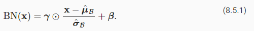
In (8.5.1), μ^B is the sample mean and σ^B is the sample standard deviation of the minibatch B. After applying standardization, the resulting minibatch has zero mean and unit variance. The choice of unit variance (vs. some other magic number) is an arbitrary choice. We recover this degree of freedom by including an elementwise scale parameter γ and shift parameter B that have the same shape as x. Both are parameters that need to be learned as part of model training.
(8.5.1)에서 μ^B는 표본 평균이고 σ^B는 미니 배치 B의 표본 표준 편차입니다. 표준화를 적용한 후 결과 미니 배치는 평균이 0이고 단위 분산이 있습니다. 단위 분산(다른 매직 넘버와 비교하여)의 선택은 임의의 선택입니다. 우리는 x와 같은 모양을 가진 요소별 척도 매개변수 γ와 이동 매개변수 B를 포함하여 이 자유도를 복구합니다. 둘 다 모델 학습의 일부로 학습해야 하는 매개변수입니다.
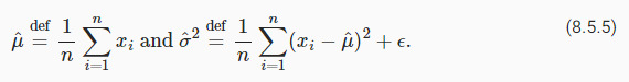
The variable magnitudes for intermediate layers cannot diverge during training since batch normalization actively centers and rescales them back to a given mean and size (via μ^B and σ^B). Practical experience confirms that, as alluded to when discussing feature rescaling, batch normalization seems to allow for more aggressive learning rates. We calculate μ^B and σ^B in (8.5.1) as follows:
중간 레이어의 변수 크기는 훈련 중에 발산할 수 없습니다. 배치 정규화가 능동적으로 중앙에 배치하고 주어진 평균 및 크기로 재조정하기 때문입니다(μ^B 및 σ^B를 통해). 실제 경험에 따르면 기능 크기 조정을 논의할 때 언급했듯이 배치 정규화가 보다 공격적인 학습 속도를 허용하는 것으로 보입니다. (8.5.1)에서 μ^B 및 σ^B를 다음과 같이 계산합니다.

Note that we add a small constant ϵ>0 to the variance estimate to ensure that we never attempt division by zero, even in cases where the empirical variance estimate might be very small or even vanish. The estimates μ^B and σ^B counteract the scaling issue by using noisy estimates of mean and variance. You might think that this noisiness should be a problem. Quite to the contrary, this is actually beneficial.
경험적 분산 추정이 매우 작거나 심지어 사라질 수 있는 경우에도 0으로 나누기를 시도하지 않도록 분산 추정에 작은 상수 ϵ>0을 추가합니다. 추정치 μ^B 및 σ^B는 평균 및 분산의 노이즈 추정치를 사용하여 스케일링 문제에 대응합니다. 이 소음이 문제가 되어야 한다고 생각할 수도 있습니다. 오히려 이것은 실제로 유익합니다.
This turns out to be a recurring theme in deep learning. For reasons that are not yet well-characterized theoretically, various sources of noise in optimization often lead to faster training and less overfitting: this variation appears to act as a form of regularization. Teye et al. (2018) and Luo et al. (2018) related the properties of batch normalization to Bayesian priors and penalties, respectively. In particular, this sheds some light on the puzzle of why batch normalization works best for moderate minibatches sizes in the 50∼100 range. This particular size of minibatch seems to inject just the “right amount” of noise per layer, both in terms of scale via σ^, and in terms of offset via μ^: a larger minibatch regularizes less due to the more stable estimates, whereas tiny minibatches destroy useful signal due to high variance. Exploring this direction further, considering alternative types of preprocessing and filtering may yet lead to other effective types of regularization.
이것은 딥 러닝에서 되풀이되는 주제로 밝혀졌습니다. 이론적으로 아직 잘 특성화되지 않은 이유로 인해 최적화에서 다양한 노이즈 소스는 종종 더 빠른 훈련과 덜 과대적합으로 이어집니다. 이러한 변형은 정규화의 한 형태로 작용하는 것으로 보입니다. Teyeet al. (2018) 및 Luo et al. (2018)은 배치 정규화의 속성을 각각 베이지안 사전 및 페널티와 관련시켰습니다. 특히 이것은 배치 정규화가 50~100 범위의 적당한 미니배치 크기에 가장 적합한 이유에 대한 퍼즐에 약간의 빛을 제공합니다. 미니배치의 이 특정 크기는 σ^를 통한 스케일과 μ^를 통한 오프셋 측면 모두에서 레이어당 "적절한 양"의 노이즈를 주입하는 것으로 보입니다. 작은 미니 배치는 높은 분산으로 인해 유용한 신호를 파괴합니다. 다른 유형의 전처리 및 필터링을 고려하여 이 방향을 더 탐색하면 다른 효과적인 유형의 정규화로 이어질 수 있습니다.
Fixing a trained model, you might think that we would prefer using the entire dataset to estimate the mean and variance. Once training is complete, why would we want the same image to be classified differently, depending on the batch in which it happens to reside? During training, such exact calculation is infeasible because the intermediate variables for all data examples change every time we update our model. However, once the model is trained, we can calculate the means and variances of each layer’s variables based on the entire dataset. Indeed this is standard practice for models employing batch normalization and thus batch normalization layers function differently in training mode (normalizing by minibatch statistics) and in prediction mode (normalizing by dataset statistics). In this form they closely resemble the behavior of dropout regularization of Section 5.6, where noise is only injected during training.
훈련된 모델을 수정하면 평균과 분산을 추정하기 위해 전체 데이터 세트를 사용하는 것이 더 좋다고 생각할 수 있습니다. 학습이 완료되면 배치에 따라 동일한 이미지를 다르게 분류해야 하는 이유는 무엇입니까? 학습 중에는 모델을 업데이트할 때마다 모든 데이터 예제의 중간 변수가 변경되기 때문에 이러한 정확한 계산은 불가능합니다. 그러나 모델이 훈련되면 전체 데이터 세트를 기반으로 각 계층 변수의 평균과 분산을 계산할 수 있습니다. 실제로 이것은 배치 정규화를 사용하는 모델의 표준 사례이므로 배치 정규화 계층은 교육 모드(미니배치 통계로 정규화)와 예측 모드(데이터 세트 통계로 정규화)에서 다르게 작동합니다. 이 형태에서 노이즈는 학습 중에만 주입되는 섹션 5.6의 드롭아웃 정규화 동작과 매우 유사합니다.
Batch Normalization 이란?
In deep learning, Batch Normalization (BN) is a technique used to improve the training process and stability of neural networks. It was proposed to address the problem of internal covariate shift, which occurs when the distribution of the inputs to a layer changes during training.
딥 러닝에서 배치 정규화(Batch Normalization, BN)은 신경망의 학습 과정과 안정성을 향상시키기 위한 기법입니다. 이 기법은 내부 공변량 변화(Internal Covariate Shift)라는 문제를 해결하기 위해 제안되었습니다. 내부 공변량 변화란, 신경망의 각 층의 입력 분포가 학습 중에 크게 변하는 현상을 의미합니다.
During the training of deep neural networks, the distribution of the activations in each layer can change significantly due to updates in the model's parameters during the optimization process. This can slow down training and make it harder for the model to converge to good solutions. Batch Normalization addresses this issue by normalizing the activations of each layer across mini-batches of data during training.
딥 뉴럴 네트워크를 학습할 때, 최적화 과정에서 모델의 매개변수가 업데이트되면서 각 층의 활성화 분포가 크게 변할 수 있습니다. 이는 학습 속도를 느리게 하고 모델이 좋은 솔루션으로 수렴하기 어렵게 만듭니다. 배치 정규화는 학습 과정에서 각 층의 활성화를 미니 배치 단위로 정규화하여 이 문제를 해결합니다.
The Batch Normalization algorithm works as follows:
배치 정규화 알고리즘의 동작은 다음과 같습니다:
- For each mini-batch of data during training, the mean and variance of the activations in each layer are computed.
학습 과정에서 각 미니 배치에 대해 각 층의 활성화의 평균과 분산을 계산합니다. - The activations are then normalized by subtracting the mean and dividing by the square root of the variance. This step ensures that the activations have a mean close to zero and a standard deviation close to one.
그런 다음 활성화를 정규화하기 위해 평균을 빼고 분산의 제곱근으로 나눕니다. 이 단계는 활성화의 평균이 거의 0이 되고 표준 편차가 거의 1이 되도록 합니다. - The normalized activations are then scaled and shifted using learnable parameters (gamma and beta) to allow the model to learn the optimal scale and shift for each activation.
정규화된 활성화는 가중치와 편향을 이용해 스케일링과 시프트됩니다. 이러한 가중치와 편향은 모델이 각 활성화에 대해 최적의 스케일과 시프트를 학습할 수 있게 합니다.
The benefits of Batch Normalization include:
배치 정규화의 이점은 다음과 같습니다:
- Improved training speed: Normalizing the activations helps to reduce internal covariate shift, which can speed up the training process and allow for the use of higher learning rates.
학습 속도 향상: 정규화된 활성화는 내부 공변량 변화를 줄여 학습 속도를 향상시키고 더 높은 학습률을 사용할 수 있게 합니다. - Increased stability: Batch Normalization can make the optimization process more stable, making it less likely for the model to diverge or get stuck in poor local minima.
안정성 향상: 배치 정규화는 최적화 과정을 더 안정적으로 만들어 모델이 발산하거나 나쁜 지역 최솟값에 빠지는 것을 방지합니다. - Regularization: Batch Normalization acts as a form of regularization by adding some noise to the activations during training, which can help prevent overfitting.
정규화 효과: 배치 정규화는 활성화에 약간의 노이즈를 추가하여 정규화의 역할을 하며, 과적합을 방지하는데 도움을 줍니다.
Batch Normalization has become a standard component in most deep neural network architectures and is widely used in various tasks such as image classification, object detection, and natural language processing.
배치 정규화는 현재 대부분의 딥 뉴럴 네트워크 구조에서 표준 구성 요소가 되어 있으며, 이미지 분류, 객체 검출, 자연어 처리 등 다양한 작업에 널리 사용됩니다.
8.5.2. Batch Normalization Layers
Batch normalization implementations for fully connected layers and convolutional layers are slightly different. One key difference between batch normalization and other layers is that because batch normalization operates on a full minibatch at a time, we cannot just ignore the batch dimension as we did before when introducing other layers.
완전 연결 계층과 컨벌루션 계층에 대한 배치 정규화 구현은 약간 다릅니다. 배치 정규화와 다른 레이어의 주요 차이점 중 하나는 배치 정규화가 한 번에 전체 미니배치에서 작동하기 때문에 이전에 다른 레이어를 도입할 때 했던 것처럼 배치 차원을 무시할 수 없다는 것입니다.
8.5.2.1. Fully Connected Layers
When applying batch normalization to fully connected layers, the original paper inserted batch normalization after the affine transformation and before the nonlinear activation function. Later applications experimented with inserting batch normalization right after activation functions (Ioffe and Szegedy, 2015). Denoting the input to the fully connected layer by x, the affine transformation by Wx+b (with the weight parameter W and the bias parameter b), and the activation function by ϕ, we can express the computation of a batch-normalization-enabled, fully connected layer output ℎ as follows:
완전 연결 레이어에 배치 정규화를 적용할 때 원본 논문에서는 아핀 변환 후와 비선형 활성화 함수 전에 배치 정규화를 삽입했습니다. 이후 애플리케이션에서는 활성화 함수 바로 뒤에 배치 정규화를 삽입하는 실험을 했습니다(Ioffe and Szegedy, 2015). 완전 연결 레이어에 대한 입력을 x, 아핀 변환을 Wx+b(가중 매개변수 W 및 편향 매개변수 b 사용), 활성화 함수를 φ로 나타내면 배치 정규화가 가능한 계산을 다음과 같이 표현할 수 있습니다. , 완전히 연결된 레이어 출력 ℎ은 다음과 같습니다.

Recall that mean and variance are computed on the same minibatch on which the transformation is applied.
평균과 분산은 변환이 적용된 동일한 미니배치에서 계산됩니다.
8.5.2.2. Convolutional Layers
Similarly, with convolutional layers, we can apply batch normalization after the convolution and before the nonlinear activation function. The key difference from batch normalization in fully connected layers is that we apply the operation on a per-channel basis across all locations. This is compatible with our assumption of translation invariance that led to convolutions: we assumed that the specific location of a pattern within an image was not critical for the purpose of understanding.
마찬가지로 컨볼루션 레이어를 사용하면 컨볼루션 이후와 비선형 활성화 함수 이전에 배치 정규화를 적용할 수 있습니다. 완전히 연결된 레이어의 배치 정규화와 주요 차이점은 모든 위치에서 채널별로 작업을 적용한다는 것입니다. 이는 컨볼루션으로 이어지는 변환 불변성 가정과 호환됩니다. 이미지 내 패턴의 특정 위치가 이해 목적에 중요하지 않다고 가정했습니다.
Assume that our minibatches contain m examples and that for each channel, the output of the convolution has height p and width q. For convolutional layers, we carry out each batch normalization over the m⋅p⋅q elements per output channel simultaneously. Thus, we collect the values over all spatial locations when computing the mean and variance and consequently apply the same mean and variance within a given channel to normalize the value at each spatial location. Each channel has its own scale and shift parameters, both of which are scalars.
미니배치가 m개의 예제를 포함하고 각 채널에 대한 컨볼루션 출력의 높이가 p이고 너비가 q라고 가정합니다. 컨벌루션 레이어의 경우 출력 채널당 m⋅p⋅q 요소에 대해 각 배치 정규화를 동시에 수행합니다. 따라서 평균과 분산을 계산할 때 모든 공간 위치에 대한 값을 수집하고 결과적으로 주어진 채널 내에서 동일한 평균과 분산을 적용하여 각 공간 위치에서 값을 정규화합니다. 각 채널에는 자체 스케일 및 시프트 매개변수가 있으며 둘 다 스칼라입니다.
8.5.2.3. Layer Normalization
Note that in the context of convolutions the batch normalization is well-defined even for minibatches of size 1: after all, we have all the locations across an image to average. Consequently, mean and variance are well defined, even if it is just within a single observation. This consideration led Ba et al. (2016) to introduce the notion of layer normalization. It works just like a batch norm, only that it is applied to one observation at a time. Consequently both the offset and the scaling factor are scalars. Given an n-dimensional vector x layer norms are given by
회선의 맥락에서 배치 정규화는 크기 1의 미니배치에 대해서도 잘 정의되어 있습니다. 결국 이미지 전체의 모든 위치를 평균화할 수 있습니다. 결과적으로 평균과 분산은 단일 관측치 내에 있더라도 잘 정의됩니다. 이러한 고려 사항은 Ba et al. (2016) 레이어 정규화의 개념을 소개합니다. 배치 표준처럼 작동하지만 한 번에 하나의 관측치에만 적용됩니다. 결과적으로 오프셋과 배율 인수는 모두 스칼라입니다. 주어진 n차원 벡터 x 레이어 규범은 다음과 같이 지정됩니다.
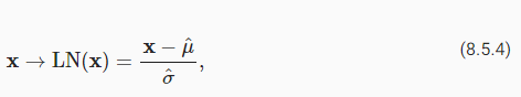
where scaling and offset are applied coefficient-wise and given by
여기서 스케일링 및 오프셋은 계수별로 적용되며 다음과 같이 지정됩니다.
As before we add a small offset ε>0 to prevent division by zero. One of the major benefits of using layer normalization is that it prevents divergence. After all, ignoring ε, the output of the layer normalization is scale independent. That is, we have LN(x)≈LN(αx) for any choice of α≠0. This becomes an equality for |α|→∞ (the approximate equality is due to the offset ε for the variance).
이전과 마찬가지로 작은 오프셋 ε>0을 추가하여 0으로 나누는 것을 방지합니다. 계층 정규화 사용의 주요 이점 중 하나는 발산을 방지한다는 것입니다. 결국, ε을 무시하면 레이어 정규화의 출력은 스케일에 독립적입니다. 즉, α≠0을 선택하는 경우 LN(x)≈LN(αx)가 있습니다. 이는 |α|→∞에 대한 등식이 됩니다(대략적인 등식은 분산에 대한 오프셋 ε 때문입니다).
Layer Normalization 이란?
딥 러닝에서 레이어 정규화(Layer Normalization, LN)은 배치 정규화와 마찬가지로 내부 공변량 변화(Internal Covariate Shift)를 해결하기 위해 제안된 정규화 기법입니다. 내부 공변량 변화란, 신경망의 각 층의 입력 분포가 학습 중에 크게 변하는 현상을 의미합니다. 배치 정규화는 미니 배치 단위로 정규화하지만, 레이어 정규화는 미니 배치가 아니라 층 내에서 정규화를 수행합니다.
레이어 정규화 알고리즘의 동작은 다음과 같습니다:
- 학습 과정에서 각 층의 활성화에 대해 평균과 분산을 계산합니다.
- 그런 다음 활성화를 정규화하기 위해 평균을 빼고 분산의 제곱근으로 나눕니다. 이 단계는 활성화의 평균이 거의 0이 되고 표준 편차가 거의 1이 되도록 합니다.
- 정규화된 활성화는 가중치와 편향을 이용해 스케일링과 시프트됩니다. 이러한 가중치와 편향은 모델이 각 활성화에 대해 최적의 스케일과 시프트를 학습할 수 있게 합니다.
레이어 정규화는 배치 크기에 상관없이 항상 일관된 정규화를 제공하므로, 배치 크기가 작거나 크더라도 안정적인 학습을 가능하게 합니다. 또한 레이어 정규화는 미니 배치의 크기가 1일 때도 사용할 수 있으며, RNN과 같은 순환 신경망에서도 적용할 수 있습니다.
레이어 정규화는 배치 정규화와 비교하여 메모리 요구량이 더 적고, 학습 시간이 더 빠르며, 미니 배치 크기에 덜 민감합니다. 따라서 최근의 딥 러닝 모델에서 레이어 정규화가 널리 사용되고 있으며, 배치 정규화와 함께 다양한 응용 분야에서 성능을 향상시키는데 기여하고 있습니다.
Internal Covariate Shift란?
내부 공변량 변화(Internal Covariate Shift)란 딥 러닝 모델의 각 층의 입력 분포가 학습 도중 크게 변하는 현상을 의미합니다. 딥 러닝 신경망은 여러 개의 층으로 구성되어 있으며, 각 층에서는 입력 데이터에 가중치를 적용하고 비선형 활성화 함수를 거쳐 출력을 계산합니다. 이렇게 여러 개의 층을 거치면서 입력 데이터의 분포가 변화하게 되는데, 이러한 변화를 내부 공변량 변화라고 합니다.
내부 공변량 변화는 심층 신경망에서 학습을 어렵게 만들 수 있습니다. 이는 두 가지 주요 이유로 발생합니다. 첫째, 각 층마다 입력 데이터의 분포가 변화하면 학습 과정에서 각 층을 통과한 출력의 분포도 달라집니다. 이는 가중치 업데이트를 어렵게 하며, 학습이 불안정해지게 합니다. 둘째, 내부 공변량 변화는 각 층의 가중치를 재사용하기 어렵게 만들어, 효과적인 학습을 어렵게 합니다.
이러한 내부 공변량 변화를 해결하는 방법으로 배치 정규화(Batch Normalization)과 레이어 정규화(Layer Normalization) 등의 정규화 기법이 제안되었습니다. 이러한 정규화 기법은 각 층의 입력 데이터의 분포를 안정화시켜 학습을 원활하게 만들어주고, 심층 신경망의 학습을 향상시키는데 기여합니다. 내부 공변량 변화의 해결은 딥 러닝 모델의 안정적인 학습과 성능 향상을 위해 중요한 문제 중 하나입니다.
8.5.2.4. Batch Normalization During Prediction
As we mentioned earlier, batch normalization typically behaves differently in training mode and prediction mode. First, the noise in the sample mean and the sample variance arising from estimating each on minibatches are no longer desirable once we have trained the model. Second, we might not have the luxury of computing per-batch normalization statistics. For example, we might need to apply our model to make one prediction at a time.
앞서 언급했듯이 배치 정규화는 일반적으로 훈련 모드와 예측 모드에서 다르게 작동합니다. 첫째, 샘플 평균의 노이즈와 미니 배치에서 각각을 추정하여 발생하는 샘플 분산은 모델을 훈련한 후에는 더 이상 바람직하지 않습니다. 둘째, 배치당 정규화 통계를 계산할 여유가 없을 수도 있습니다. 예를 들어 한 번에 하나의 예측을 수행하기 위해 모델을 적용해야 할 수 있습니다.
Typically, after training, we use the entire dataset to compute stable estimates of the variable statistics and then fix them at prediction time. Consequently, batch normalization behaves differently during training and at test time. Recall that dropout also exhibits this characteristic.
일반적으로 교육 후 전체 데이터 세트를 사용하여 변수 통계의 안정적인 추정치를 계산한 다음 예측 시간에 수정합니다. 결과적으로 배치 정규화는 훈련 중과 테스트 중에 다르게 작동합니다. 드롭아웃도 이러한 특성을 나타냄을 상기하십시오.
8.5.3. Implementation from Scratch
To see how batch normalization works in practice, we implement one from scratch below.
배치 정규화가 실제로 어떻게 작동하는지 확인하기 위해 아래에서 하나를 처음부터 구현합니다.
def batch_norm(X, gamma, beta, moving_mean, moving_var, eps, momentum):
    # Use is_grad_enabled to determine whether we are in training mode
    if not torch.is_grad_enabled():
        # In prediction mode, use mean and variance obtained by moving average
        X_hat = (X - moving_mean) / torch.sqrt(moving_var + eps)
    else:
        assert len(X.shape) in (2, 4)
        if len(X.shape) == 2:
            # When using a fully connected layer, calculate the mean and
            # variance on the feature dimension
            mean = X.mean(dim=0)
            var = ((X - mean) ** 2).mean(dim=0)
        else:
            # When using a two-dimensional convolutional layer, calculate the
            # mean and variance on the channel dimension (axis=1). Here we
            # need to maintain the shape of X, so that the broadcasting
            # operation can be carried out later
            mean = X.mean(dim=(0, 2, 3), keepdim=True)
            var = ((X - mean) ** 2).mean(dim=(0, 2, 3), keepdim=True)
        # In training mode, the current mean and variance are used
        X_hat = (X - mean) / torch.sqrt(var + eps)
        # Update the mean and variance using moving average
        moving_mean = (1.0 - momentum) * moving_mean + momentum * mean
        moving_var = (1.0 - momentum) * moving_var + momentum * var
    Y = gamma * X_hat + beta  # Scale and shift
    return Y, moving_mean.data, moving_var.data
위 코드는 배치 정규화(Batch Normalization) 기능을 수행하는 함수를 정의한 것입니다. 배치 정규화는 딥 러닝 모델에서 내부 공변량 변화(Internal Covariate Shift)를 해결하고 학습을 안정화시키기 위해 사용되는 기법 중 하나입니다.
이 함수에서 사용되는 인자들은 다음과 같습니다.
- X: 입력 데이터
- gamma: 스케일(scale) 파라미터
- beta: 시프트(shift) 파라미터
- moving_mean: 이동 평균(Moving Average)을 저장하기 위한 변수
- moving_var: 이동 분산(Moving Variance)을 저장하기 위한 변수
- eps: 분모가 0이 되는 것을 방지하기 위한 작은 값(epsilon)
- momentum: 이동 평균과 이동 분산을 업데이트할 때 사용되는 모멘텀 파라미터
함수의 동작은 다음과 같습니다.
- torch.is_grad_enabled() 함수를 사용하여 현재 학습 모드인지 판단합니다.
- 학습 모드가 아닐 경우(예측 모드), 이동 평균과 이동 분산을 사용하여 정규화된 데이터 X_hat을 계산합니다.
- 학습 모드일 경우, 입력 데이터 X의 shape에 따라 평균(mean)과 분산(var)을 계산합니다. Fully connected layer인 경우 feature 차원을 기준으로, 2D 합성곱(Convolutional) layer인 경우 채널 차원을 기준으로 평균과 분산을 계산합니다.
- 학습 모드일 경우, 계산된 평균과 분산을 사용하여 X를 정규화하고, 이동 평균과 이동 분산을 업데이트합니다.
- 최종적으로 정규화된 X_hat에 스케일(gamma)과 시프트(beta)를 적용하여 최종 결과 Y를 반환합니다.
이렇게 배치 정규화는 입력 데이터의 분포를 안정화시키고 학습을 더욱 안정적으로 만들어주는 기법으로 널리 사용됩니다. 주로 딥 러닝 모델의 층 사이에 배치 정규화를 추가하여 학습을 개선하는데 사용됩니다.
We can now create a proper BatchNorm layer. Our layer will maintain proper parameters for scale gamma and shift beta, both of which will be updated in the course of training. Additionally, our layer will maintain moving averages of the means and variances for subsequent use during model prediction.
이제 적절한 BatchNorm 레이어를 생성할 수 있습니다. 우리 레이어는 스케일 감마 및 시프트 베타에 대한 적절한 매개 변수를 유지하며 둘 다 교육 과정에서 업데이트됩니다. 또한 레이어는 모델 예측 중에 후속 사용을 위해 평균 및 분산의 이동 평균을 유지합니다.
Putting aside the algorithmic details, note the design pattern underlying our implementation of the layer. Typically, we define the mathematics in a separate function, say batch_norm. We then integrate this functionality into a custom layer, whose code mostly addresses bookkeeping matters, such as moving data to the right device context, allocating and initializing any required variables, keeping track of moving averages (here for mean and variance), and so on. This pattern enables a clean separation of mathematics from boilerplate code. Also note that for the sake of convenience we did not worry about automatically inferring the input shape here, thus we need to specify the number of features throughout. By now all modern deep learning frameworks offer automatic detection of size and shape in the high-level batch normalization APIs (in practice we will use this instead).
알고리즘 세부 사항은 제쳐두고 레이어 구현의 기본 디자인 패턴에 주목하십시오. 일반적으로 별도의 함수인 batch_norm에서 수학을 정의합니다. 그런 다음 이 기능을 사용자 지정 계층에 통합합니다. 이 계층의 코드는 데이터를 올바른 장치 컨텍스트로 이동, 필요한 변수 할당 및 초기화, 이동 평균 추적(여기서는 평균 및 분산) 등과 같은 부기 문제를 주로 처리합니다. . 이 패턴을 사용하면 상용구 코드에서 수학을 깔끔하게 분리할 수 있습니다. 또한 편의를 위해 여기에서 입력 모양을 자동으로 유추하는 것에 대해 걱정하지 않았으므로 전체 기능의 수를 지정해야 합니다. 지금까지 모든 최신 딥 러닝 프레임워크는 높은 수준의 배치 정규화 API에서 크기와 모양을 자동으로 감지합니다(실제로는 이를 대신 사용함).
class BatchNorm(nn.Module):
    # num_features: the number of outputs for a fully connected layer or the
    # number of output channels for a convolutional layer. num_dims: 2 for a
    # fully connected layer and 4 for a convolutional layer
    def __init__(self, num_features, num_dims):
        super().__init__()
        if num_dims == 2:
            shape = (1, num_features)
        else:
            shape = (1, num_features, 1, 1)
        # The scale parameter and the shift parameter (model parameters) are
        # initialized to 1 and 0, respectively
        self.gamma = nn.Parameter(torch.ones(shape))
        self.beta = nn.Parameter(torch.zeros(shape))
        # The variables that are not model parameters are initialized to 0 and
        # 1
        self.moving_mean = torch.zeros(shape)
        self.moving_var = torch.ones(shape)

    def forward(self, X):
        # If X is not on the main memory, copy moving_mean and moving_var to
        # the device where X is located
        if self.moving_mean.device != X.device:
            self.moving_mean = self.moving_mean.to(X.device)
            self.moving_var = self.moving_var.to(X.device)
        # Save the updated moving_mean and moving_var
        Y, self.moving_mean, self.moving_var = batch_norm(
            X, self.gamma, self.beta, self.moving_mean,
            self.moving_var, eps=1e-5, momentum=0.1)
        return Y
위 코드는 배치 정규화를 수행하는 사용자 정의 클래스인 BatchNorm을 정의한 것입니다. 배치 정규화는 딥 러닝 모델에서 내부 공변량 변화(Internal Covariate Shift)를 줄이고 학습을 안정화시키기 위해 사용되는 기법 중 하나입니다.
클래스의 생성자(__init__)에서는 다음과 같은 인자들을 받습니다:
- num_features: fully connected layer의 출력 뉴런 수 또는 합성곱 레이어의 출력 채널 수
- num_dims: fully connected layer의 경우 2, 합성곱 레이어의 경우 4
클래스의 동작은 다음과 같습니다:
- 생성자에서 스케일 파라미터 gamma와 시프트 파라미터 beta를 초기화합니다. 이들은 모델의 학습 가능한 파라미터로 선언되며, nn.Parameter를 사용하여 정의됩니다. 초기값으로는 스케일 파라미터 gamma는 1로 초기화하고, 시프트 파라미터 beta는 0으로 초기화합니다.
- 이동 평균과 이동 분산을 저장할 변수 self.moving_mean과 self.moving_var를 정의합니다. 이들은 학습 가능한 파라미터가 아니며, 초기값으로는 이동 평균을 0으로, 이동 분산을 1로 설정합니다.
- 클래스의 forward 메서드에서는 입력 데이터 X에 대해 배치 정규화를 수행합니다. 이 때, 이동 평균과 이동 분산은 이전 단계에서 업데이트된 값을 사용합니다.
- 만약 입력 데이터 X가 주 메모리에 있지 않은 경우, 이동 평균과 이동 분산을 X와 동일한 디바이스로 복사합니다.
- batch_norm 함수를 호출하여 X를 정규화하고, 결과로 스케일과 시프트가 적용된 Y를 얻습니다. 이 때, 이동 평균과 이동 분산은 업데이트된 값으로 갱신됩니다.
- 최종적으로 스케일과 시프트가 적용된 정규화된 데이터 Y를 반환합니다.
이렇게 BatchNorm 클래스를 사용하면 배치 정규화를 쉽게 사용할 수 있으며, 딥 러닝 모델의 학습과 안정화에 도움이 됩니다.
We used momentum to govern the aggregation over past mean and variance estimates. This is somewhat of a misnomer as it has nothing whatsoever to do with the momentum term of optimization in Section 12.6. Nonetheless, it is the commonly adopted name for this term and in deference to API naming convention we use the same variable name in our code, too.
모멘텀을 사용하여 과거 평균 및 분산 추정치에 대한 집계를 관리했습니다. 이것은 섹션 12.6의 최적화의 모멘텀 항과 전혀 관련이 없기 때문에 다소 잘못된 이름입니다. 그럼에도 불구하고 이 용어에 대해 일반적으로 채택되는 이름이며 API 명명 규칙에 따라 코드에서도 동일한 변수 이름을 사용합니다.
8.5.4. LeNet with Batch Normalization
To see how to apply BatchNorm in context, below we apply it to a traditional LeNet model (Section 7.6). Recall that batch normalization is applied after the convolutional layers or fully connected layers but before the corresponding activation functions.
컨텍스트에서 BatchNorm을 적용하는 방법을 확인하기 위해 아래에서 이를 기존 LeNet 모델에 적용합니다(섹션 7.6). 배치 정규화는 컨벌루션 계층 또는 완전 연결 계층 이후에 적용되지만 해당 활성화 함수 이전에 적용됩니다.
class BNLeNetScratch(d2l.Classifier):
    def __init__(self, lr=0.1, num_classes=10):
        super().__init__()
        self.save_hyperparameters()
        self.net = nn.Sequential(
            nn.LazyConv2d(6, kernel_size=5), BatchNorm(6, num_dims=4),
            nn.Sigmoid(), nn.AvgPool2d(kernel_size=2, stride=2),
            nn.LazyConv2d(16, kernel_size=5), BatchNorm(16, num_dims=4),
            nn.Sigmoid(), nn.AvgPool2d(kernel_size=2, stride=2),
            nn.Flatten(), nn.LazyLinear(120),
            BatchNorm(120, num_dims=2), nn.Sigmoid(), nn.LazyLinear(84),
            BatchNorm(84, num_dims=2), nn.Sigmoid(),
            nn.LazyLinear(num_classes))
위 코드는 Scratch에서 학습하는 Batch Normalization을 적용한 LeNet과 같은 모델인 BNLeNetScratch 클래스를 정의하는 것입니다.
BNLeNetScratch 클래스의 생성자(__init__)에서는 다음과 같은 인자들을 받습니다:
- lr: 학습률 (기본값은 0.1)
- num_classes: 분류하고자 하는 클래스의 수 (기본값은 10)
클래스의 동작은 다음과 같습니다:
- nn.Sequential을 사용하여 모델 레이어를 순차적으로 쌓습니다.
- 첫 번째 합성곱 레이어 (nn.LazyConv2d) 다음에 배치 정규화 레이어 (BatchNorm)를 적용합니다. 이렇게 함으로써 입력 데이터의 분포를 정규화하고 학습을 안정화시킬 수 있습니다. 각 합성곱 레이어는 5x5 커널 크기를 사용하며, 첫 번째 레이어는 6개의 출력 채널을 가지고, 두 번째 레이어는 16개의 출력 채널을 가집니다.
- 배치 정규화 레이어 이후에는 활성화 함수로 시그모이드 (nn.Sigmoid())를 사용합니다.
- 평균 풀링 레이어 (nn.AvgPool2d)를 적용하여 특성 맵의 크기를 줄입니다.
- 평탄화 레이어 (nn.Flatten())를 사용하여 2D 텐서를 1D 벡터로 변환합니다.
- 완전 연결 레이어 (nn.LazyLinear)를 추가하고 배치 정규화 레이어를 적용합니다. 첫 번째 완전 연결 레이어는 120개의 출력 뉴런을 가지고, 두 번째 레이어는 84개의 출력 뉴런을 가집니다.
- 완전 연결 레이어 이후에는 다시 시그모이드 활성화 함수를 사용합니다.
- 마지막으로 완전 연결 레이어를 추가하고, 클래스의 수에 해당하는 출력 뉴런을 가지게 됩니다.
이렇게 정의된 BNLeNetScratch 클래스는 학습 가능한 모델로, 배치 정규화를 통해 학습 안정성을 증가시키고, 일반화 능력을 향상시킬 수 있습니다.
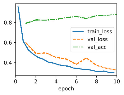
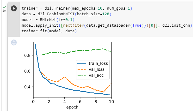
As before, we will train our network on the Fashion-MNIST dataset. This code is virtually identical to that when we first trained LeNet.
이전과 마찬가지로 Fashion-MNIST 데이터 세트에서 네트워크를 훈련할 것입니다. 이 코드는 LeNet을 처음 학습했을 때와 거의 동일합니다.
trainer = d2l.Trainer(max_epochs=10, num_gpus=1)
data = d2l.FashionMNIST(batch_size=128)
model = BNLeNetScratch(lr=0.1)
model.apply_init([next(iter(data.get_dataloader(True)))[0]], d2l.init_cnn)
trainer.fit(model, data)
위 코드는 다음과 같은 작업을 수행하는 것입니다.
- d2l.Trainer 클래스의 인스턴스를 생성합니다. Trainer는 딥러닝 모델을 학습시키기 위한 도우미 클래스로, 에폭 수(max_epochs)를 10으로 설정하고, 사용할 GPU 개수(num_gpus)를 1개로 설정합니다.
- d2l.FashionMNIST 클래스의 인스턴스를 생성하여 데이터를 로드합니다. 이 데이터셋은 패션 관련 이미지를 분류하는데 사용되며, 배치 크기(batch_size)는 128로 설정됩니다.
- BNLeNetScratch 클래스의 인스턴스를 생성합니다. 이 모델은 BNLeNetScratch(lr=0.1)로 생성되며, 학습률(lr)은 0.1로 설정됩니다.
- model.apply_init([next(iter(data.get_dataloader(True)))[0]], d2l.init_cnn)를 호출하여 모델의 파라미터를 초기화합니다. 이 함수는 BNLeNetScratch 클래스의 인스턴스 model과 데이터 로더의 첫 번째 미니배치를 사용하여, 미리 정의된 d2l.init_cnn 함수를 이용해 모델의 파라미터를 초기화합니다.
- trainer.fit(model, data)를 호출하여 모델을 학습합니다. Trainer 클래스의 fit 메서드를 사용하여 모델과 데이터를 전달하면, 지정한 에폭 수만큼 모델을 학습합니다. 학습은 미니배치 단위로 이루어지며, 지정된 에폭 수 만큼 반복하여 모델의 파라미터를 조정하면서 손실 함수를 최적화하여 모델을 훈련시킵니다.
이렇게 코드를 실행하면 BNLeNetScratch 모델이 Fashion MNIST 데이터셋에 대해 학습되고, 훈련된 모델을 사용하여 패션 관련 이미지를 분류할 수 있습니다.
Let’s have a look at the scale parameter gamma and the shift parameter beta learned from the first batch normalization layer.
첫 번째 배치 정규화 레이어에서 학습한 척도 매개변수 감마와 이동 매개변수 베타를 살펴보겠습니다.
model.net[1].gamma.reshape((-1,)), model.net[1].beta.reshape((-1,))(tensor([1.7430, 1.9467, 1.6972, 1.5474, 2.0986, 1.8447], device='cuda:0',
grad_fn=<ReshapeAliasBackward0>),
tensor([ 0.9244, -1.3682, 1.4599, -1.5325, 1.3034, -0.0391], device='cuda:0',
grad_fn=<ReshapeAliasBackward0>))위 코드는 모델의 Batch Normalization(BN) 레이어에서 사용되는 스케일 파라미터(gamma)와 시프트 파라미터(beta)를 1차원으로 변환하여 출력하는 코드입니다.
- model.net[1]: 모델(BNLeNetScratch)의 nn.Sequential에서 두 번째 레이어를 선택합니다. 두 번째 레이어는 Batch Normalization 레이어입니다.
- model.net[1].gamma: 선택된 Batch Normalization 레이어의 스케일 파라미터(gamma)를 가져옵니다. 스케일 파라미터는 학습되는 모델 파라미터이며, 각 채널(channel)마다 하나의 값이 있습니다.
- model.net[1].beta: 선택된 Batch Normalization 레이어의 시프트 파라미터(beta)를 가져옵니다. 시프트 파라미터도 스케일 파라미터와 같이 학습되는 모델 파라미터입니다.
- model.net[1].gamma.reshape((-1,)): 스케일 파라미터인 gamma를 1차원으로 변환합니다. reshape 함수를 사용하여 모든 채널의 값을 일렬로 나열합니다.
- model.net[1].beta.reshape((-1,)): 시프트 파라미터인 beta를 1차원으로 변환합니다. 마찬가지로 reshape 함수를 사용하여 모든 채널의 값을 일렬로 나열합니다.
즉, 위 코드는 Batch Normalization 레이어의 스케일 파라미터와 시프트 파라미터를 각각 1차원 벡터로 변환하여 출력합니다. 이렇게 1차원 벡터로 변환하는 이유는, 이후에 이 스케일 파라미터와 시프트 파라미터를 사용하여 테스트 데이터에 대해 Batch Normalization을 적용하기 위해서입니다. 일반적으로 테스트 시에는 미리 학습된 모델의 파라미터만 사용하므로, 학습된 스케일 파라미터와 시프트 파라미터를 사용하여 정규화를 수행합니다.
8.5.5. Concise Implementation
Compared with the BatchNorm class, which we just defined ourselves, we can use the BatchNorm class defined in high-level APIs from the deep learning framework directly. The code looks virtually identical to our implementation above, except that we no longer need to provide additional arguments for it to get the dimensions right.
방금 정의한 BatchNorm 클래스와 비교하면 딥러닝 프레임워크에서 상위 API에 정의된 BatchNorm 클래스를 직접 사용할 수 있습니다. 코드는 치수를 올바르게 가져오기 위해 더 이상 추가 인수를 제공할 필요가 없다는 점을 제외하면 위의 구현과 거의 동일합니다.
class BNLeNet(d2l.Classifier):
    def __init__(self, lr=0.1, num_classes=10):
        super().__init__()
        self.save_hyperparameters()
        self.net = nn.Sequential(
            nn.LazyConv2d(6, kernel_size=5), nn.LazyBatchNorm2d(),
            nn.Sigmoid(), nn.AvgPool2d(kernel_size=2, stride=2),
            nn.LazyConv2d(16, kernel_size=5), nn.LazyBatchNorm2d(),
            nn.Sigmoid(), nn.AvgPool2d(kernel_size=2, stride=2),
            nn.Flatten(), nn.LazyLinear(120), nn.LazyBatchNorm1d(),
            nn.Sigmoid(), nn.LazyLinear(84), nn.LazyBatchNorm1d(),
            nn.Sigmoid(), nn.LazyLinear(num_classes))
위 코드는 Batch Normalization을 포함하는 LeNet 모델(BNLeNet)을 정의하는 코드입니다.
- nn.LazyConv2d(6, kernel_size=5): 입력 채널이 6개인 2D 컨볼루션 레이어를 생성합니다. 커널 크기는 5x5 입니다.
- nn.LazyBatchNorm2d(): 2D Batch Normalization 레이어를 생성합니다. 이 레이어는 컨볼루션 레이어의 출력에 대해 각 채널별로 정규화를 수행합니다.
- nn.Sigmoid(): Sigmoid 활성화 함수를 추가합니다.
- nn.AvgPool2d(kernel_size=2, stride=2): 2x2 크기의 평균 풀링 레이어를 생성합니다. 스트라이드는 2로 설정되어 입력 이미지의 크기를 반으로 줄입니다.
이와 같은 구조를 반복하여 모델을 정의하고, 마지막에는 클래스의 개수에 해당하는 출력 노드 개수를 가진 nn.LazyLinear(num_classes) 레이어를 추가합니다. 이 모델은 입력 이미지를 처리하여 클래스를 분류하는 데 사용됩니다. 또한 Batch Normalization 레이어가 컨볼루션 레이어와 완전 연결 레이어에 모두 사용되는 것을 볼 수 있습니다. 이렇게 Batch Normalization을 적용하여 모델의 학습 안정성을 향상시킬 수 있습니다.
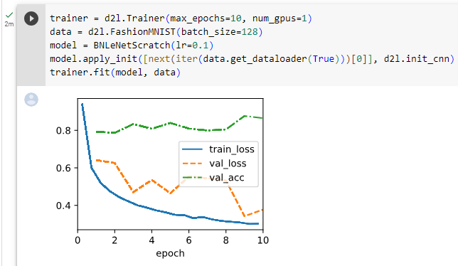
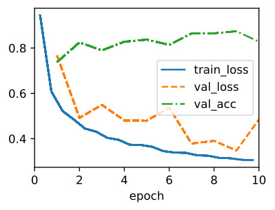
Below, we use the same hyperparameters to train our model. Note that as usual, the high-level API variant runs much faster because its code has been compiled to C++ or CUDA while our custom implementation must be interpreted by Python.
아래에서는 동일한 하이퍼파라미터를 사용하여 모델을 훈련합니다. 평소와 같이 고수준 API 변형은 코드가 C++ 또는 CUDA로 컴파일되었기 때문에 훨씬 빠르게 실행되는 반면 사용자 정의 구현은 Python으로 해석되어야 합니다.
trainer = d2l.Trainer(max_epochs=10, num_gpus=1)
data = d2l.FashionMNIST(batch_size=128)
model = BNLeNet(lr=0.1)
model.apply_init([next(iter(data.get_dataloader(True)))[0]], d2l.init_cnn)
trainer.fit(model, data)
위 코드는 BNLeNet 모델을 FashionMNIST 데이터셋으로 학습하는 과정을 보여주는 코드입니다.
- trainer = d2l.Trainer(max_epochs=10, num_gpus=1): 학습을 수행하기 위한 트레이너 객체를 생성합니다. max_epochs는 최대 학습 에포크(epoch) 수를 의미하고, num_gpus는 사용할 GPU 개수를 나타냅니다.
- data = d2l.FashionMNIST(batch_size=128): FashionMNIST 데이터셋을 생성하고 배치 크기(batch_size)를 128로 설정합니다.
- model = BNLeNet(lr=0.1): BNLeNet 모델을 생성하고, 학습률(learning rate)로 0.1을 설정합니다.
- model.apply_init([next(iter(data.get_dataloader(True)))[0]], d2l.init_cnn): 모델의 파라미터들을 초기화합니다. data.get_dataloader(True)로부터 다음 배치를 가져와 모델의 초기화에 사용합니다.
- trainer.fit(model, data): 앞서 생성한 트레이너를 사용하여 모델을 FashionMNIST 데이터셋으로 학습합니다. 학습은 최대 10 에포크 동안 진행됩니다.
이렇게 코드를 실행하면 BNLeNet 모델이 FashionMNIST 데이터셋으로 학습되고, 최대 10 에포크까지 학습이 진행됩니다. 학습이 끝나면 모델은 FashionMNIST 데이터셋의 분류 작업에 적용할 수 있습니다.
8.5.6. Discussion
Intuitively, batch normalization is thought to make the optimization landscape smoother. However, we must be careful to distinguish between speculative intuitions and true explanations for the phenomena that we observe when training deep models. Recall that we do not even know why simpler deep neural networks (MLPs and conventional CNNs) generalize well in the first place. Even with dropout and weight decay, they remain so flexible that their ability to generalize to unseen data likely needs significantly more refined learning-theoretic generalization guarantees.
직관적으로 배치 정규화는 최적화 환경을 더 매끄럽게 만드는 것으로 생각됩니다. 그러나 딥 모델을 훈련할 때 관찰하는 현상에 대한 추론적 직관과 참된 설명을 구별하는 데 주의해야 합니다. 더 간단한 심층 신경망(MLP 및 기존 CNN)이 처음부터 잘 일반화되는 이유조차 알지 못한다는 점을 상기하십시오. 드롭아웃 및 가중치 감소에도 불구하고 그들은 매우 유연하여 보이지 않는 데이터를 일반화하는 능력에는 훨씬 더 세련된 학습 이론 일반화 보장이 필요할 수 있습니다.
In the original paper proposing batch normalization (Ioffe and Szegedy, 2015), in addition to introducing a powerful and useful tool, offered an explanation for why it works: by reducing internal covariate shift. Presumably by internal covariate shift the authors meant something like the intuition expressed above—the notion that the distribution of variable values changes over the course of training. However, there were two problems with this explanation: i) This drift is very different from covariate shift, rendering the name a misnomer. If anything, it is closer to concept drift. ii) The explanation offers an under-specified intuition but leaves the question of why precisely this technique works an open question wanting for a rigorous explanation. Throughout this book, we aim to convey the intuitions that practitioners use to guide their development of deep neural networks. However, we believe that it is important to separate these guiding intuitions from established scientific fact. Eventually, when you master this material and start writing your own research papers you will want to be clear to delineate between technical claims and hunches.
배치 정규화를 제안하는 원본 논문(Ioffe and Szegedy, 2015)에서 강력하고 유용한 도구를 소개하는 것 외에도 내부 공변량 이동을 줄임으로써 작동하는 이유에 대한 설명을 제공했습니다. 아마도 내부 공변량 이동에 의해 저자는 위에서 표현된 직관과 같은 것을 의미했습니다. 즉, 변수 값의 분포가 훈련 과정에서 변경된다는 개념입니다. 그러나이 설명에는 두 가지 문제가 있습니다. i) 이 드리프트는 공변량 이동과 매우 다르기 때문에 이름이 잘못되었습니다. 오히려 개념 드리프트에 가깝다. ii) 설명은 덜 구체화된 직관을 제공하지만 정확히 이 기술이 작동하는 이유에 대한 질문을 엄격한 설명이 필요한 열린 질문으로 남겨 둡니다. 이 책 전체에서 우리는 실무자가 심층 신경망 개발을 안내하는 데 사용하는 직관을 전달하는 것을 목표로 합니다. 그러나 우리는 이러한 직관을 확립된 과학적 사실과 분리하는 것이 중요하다고 믿습니다. 결국, 이 자료를 마스터하고 자신의 연구 논문을 작성하기 시작할 때 기술적 주장과 직감을 명확하게 구분하고 싶을 것입니다.
Following the success of batch normalization, its explanation in terms of internal covariate shift has repeatedly surfaced in debates in the technical literature and broader discourse about how to present machine learning research. In a memorable speech given while accepting a Test of Time Award at the 2017 NeurIPS conference, Ali Rahimi used internal covariate shift as a focal point in an argument likening the modern practice of deep learning to alchemy. Subsequently, the example was revisited in detail in a position paper outlining troubling trends in machine learning (Lipton and Steinhardt, 2018). Other authors have proposed alternative explanations for the success of batch normalization, some claiming that batch normalization’s success comes despite exhibiting behavior that is in some ways opposite to those claimed in the original paper (Santurkar et al., 2018).
배치 정규화의 성공에 따라 내부 공변량 변화에 대한 설명이 기계 학습 연구를 제시하는 방법에 대한 기술 문헌 및 광범위한 담론에서 반복적으로 표면화되었습니다. 2017 NeurIPS 컨퍼런스에서 Test of Time Award를 수상하면서 기억에 남는 연설에서 Ali Rahimi는 딥 러닝의 현대적 관행을 연금술에 비유하는 논쟁에서 내부 공변량 이동을 초점으로 사용했습니다. 그 후, 기계 학습의 문제가 되는 추세를 요약한 입장 문서에서 이 예를 자세히 다시 검토했습니다(Lipton and Steinhardt, 2018). 다른 저자들은 배치 정규화의 성공에 대한 대안적인 설명을 제안했으며, 일부는 원래 논문에서 주장한 것과 반대되는 행동을 보임에도 불구하고 배치 정규화의 성공이 왔다고 주장했습니다(Santurkar et al., 2018).
We note that the internal covariate shift is no more worthy of criticism than any of thousands of similarly vague claims made every year in the technical machine learning literature. Likely, its resonance as a focal point of these debates owes to its broad recognizability to the target audience. Batch normalization has proven an indispensable method, applied in nearly all deployed image classifiers, earning the paper that introduced the technique tens of thousands of citations. We conjecture, though, that the guiding principles of regularization through noise injection, acceleration through rescaling and lastly preprocessing may well lead to further inventions of layers and techniques in the future.
우리는 내부 공변량 변화가 기술 기계 학습 문헌에서 매년 제기되는 유사하게 모호한 수천 건의 주장보다 더 이상 비판할 가치가 없다는 점에 주목합니다. 아마도 이러한 논쟁의 초점으로서의 공명은 대상 청중에 대한 광범위한 인식 가능성 때문일 것입니다. 배치 정규화는 배포된 거의 모든 이미지 분류기에 적용되는 필수적인 방법으로 입증되었으며, 이 기술을 소개한 논문은 수만 번 인용되었습니다. 그러나 잡음 주입을 통한 정규화, 크기 조정을 통한 가속 및 마지막으로 전처리의 기본 원리는 향후 레이어 및 기술의 추가 발명으로 이어질 수 있다고 추측합니다.
On a more practical note, there are a number of aspects worth remembering about batch normalization:
보다 실용적으로 배치 정규화에 대해 기억할 가치가 있는 여러 측면이 있습니다.
- During model training, batch normalization continuously adjusts the intermediate output of the network by utilizing the mean and standard deviation of the minibatch, so that the values of the intermediate output in each layer throughout the neural network are more stable.
- 모델 학습 중에 배치 정규화는 미니배치의 평균과 표준편차를 활용하여 네트워크의 중간 출력을 지속적으로 조정하여 신경망 전체의 각 계층의 중간 출력 값이 보다 안정적이 되도록 합니다.
- Batch normalization for fully connected layers and convolutional layers are slightly different. In fact, for convolutional layers, layer normalization can sometimes be used as an alternative.
- 완전 연결 계층과 컨벌루션 계층의 배치 정규화는 약간 다릅니다. 실제로 컨볼루션 레이어의 경우 레이어 정규화가 때때로 대안으로 사용될 수 있습니다.
- Like a dropout layer, batch normalization layers have different behaviors in training mode and prediction mode.
- 드롭아웃 레이어와 마찬가지로 배치 정규화 레이어는 훈련 모드와 예측 모드에서 서로 다른 동작을 합니다.
- Batch normalization is useful for regularization and improving convergence in optimization. On the other hand, the original motivation of reducing internal covariate shift seems not to be a valid explanation.
- 배치 정규화는 최적화에서 정규화 및 수렴 개선에 유용합니다. 반면에 내부 공변량 이동을 줄이려는 원래 동기는 유효한 설명이 아닌 것 같습니다.
- For more robust models that are less sensitive to input perturbations, consider removing batch normalization (Wang et al., 2022).
- 입력 섭동에 덜 민감한 보다 강력한 모델의 경우 배치 정규화를 제거하는 것이 좋습니다(Wang et al., 2022).
8.5.7. Exercises
- Should we remove the bias parameter from the fully connected layer or the convolutional layer before the batch normalization? Why?
- Compare the learning rates for LeNet with and without batch normalization.
- Plot the increase in validation accuracy.
- How large can you make the learning rate before the optimization fails in both cases?
- Do we need batch normalization in every layer? Experiment with it?
- Implement a “lite” version of batch normalization that only removes the mean, or alternatively one that only removes the variance. How does it behave?
- Fix the parameters beta and gamma. Observe and analyze the results.
- Can you replace dropout by batch normalization? How does the behavior change?
- Research ideas: think of other normalization transforms that you can apply:
- Can you apply the probability integral transform?
- Can you use a full rank covariance estimate? Why should you probably not do that?
- Can you use other compact matrix variants (block-diagonal, low-displacement rank, Monarch, etc.)?
- Does a sparsification compression act as a regularizer?
- Are there other projections (e.g., convex cone, symmetry group-specific transforms) that you can use?
'Dive into Deep Learning > D2L Convolutional Neural Networks (CNN)' 카테고리의 다른 글
| D2L - 8.8. Designing Convolution Network Architectures (0) | 2023.07.18 |
|---|---|
| D2L - 8.7. Densely Connected Networks (DenseNet) (0) | 2023.07.18 |
| D2L - 8.6. Residual Networks (ResNet) and ResNeXt (0) | 2023.07.18 |
| D2L - 8.4. Multi-Branch Networks (GoogLeNet) (0) | 2023.07.18 |
| D2L - 8.3. Network in Network (NiN) (0) | 2023.07.11 |
| D2L - 8.2. Networks Using Blocks (VGG) (0) | 2023.07.10 |
| D2L - 8.1. Deep Convolutional Neural Networks (AlexNet) (0) | 2023.07.10 |
| D2L - 8. Modern Convolutional Neural Networks (0) | 2023.07.10 |
| D2L - 7.6. Convolutional Neural Networks (LeNet) (0) | 2023.07.09 |
| D2L - 7.5. Pooling (1) | 2023.07.09 |