

https://d2l.ai/chapter_convolutional-modern/cnn-design.html
8.8. Designing Convolution Network Architectures — Dive into Deep Learning 1.0.0-beta0 documentation
d2l.ai
8.8. Designing Convolution Network Architectures
The past sections took us on a tour of modern network design for computer vision. Common to all the work we covered was that it heavily relied on the intuition of scientists. Many of the architectures are heavily informed by human creativity and to a much lesser extent by systematic exploration of the design space that deep networks offer. Nonetheless, this network engineering approach has been tremendously successful.
지난 섹션에서는 컴퓨터 비전을 위한 최신 네트워크 설계를 살펴보았습니다. 우리가 다룬 모든 작업의 공통점은 과학자의 직관에 크게 의존한다는 것입니다. 많은 아키텍처는 인간의 창의성에 의해 크게 영향을 받으며 심층 네트워크가 제공하는 디자인 공간의 체계적인 탐색에 의해 훨씬 덜 영향을 받습니다. 그럼에도 불구하고 이 네트워크 엔지니어링 접근 방식은 엄청난 성공을 거두었습니다.
Since AlexNet (Section 8.1) beat conventional computer vision models on ImageNet, it became popular to construct very deep networks by stacking blocks of convolutions, all designed by the same pattern. In particular, 3×3 convolutions were popularized by VGG networks (Section 8.2). NiN (Section 8.3) showed that even 1×1 convolutions could be beneficial by adding local nonlinearities. Moreover, NiN solved the problem of aggregating information at the head of a network by aggregation across all locations. GoogLeNet (Section 8.4) added multiple branches of different convolution width, combining the advantages of VGG and NiN in its Inception block. ResNets (Section 8.6) changed the inductive bias towards the identity mapping (from f(x)=0). This allowed for very deep networks. Almost a decade later, the ResNet design is still popular, a testament to its design. Lastly, ResNeXt (Section 8.6.5) added grouped convolutions, offering a better trade-off between parameters and computation. A precursor to Transformers for vision, the Squeeze-and-Excitation Networks (SENets) allow for efficient information transfer between locations (Hu et al., 2018). They accomplished this by computing a per-channel global attention function.
AlexNet(섹션 8.1)이 ImageNet에서 기존 컴퓨터 비전 모델을 능가했기 때문에 모두 동일한 패턴으로 설계된 컨볼루션 블록을 쌓아 매우 깊은 네트워크를 구성하는 것이 인기를 얻었습니다. 특히 3×3 컨볼루션은 VGG 네트워크에 의해 대중화되었습니다(섹션 8.2). NiN(섹션 8.3)은 1×1 컨볼루션도 로컬 비선형성을 추가하면 도움이 될 수 있음을 보여주었습니다. 또한 NiN은 모든 위치에서 집계하여 네트워크 헤드에서 정보를 집계하는 문제를 해결했습니다. GoogLeNet(섹션 8.4)은 Inception 블록에서 VGG와 NiN의 장점을 결합하여 서로 다른 컨볼루션 폭의 여러 분기를 추가했습니다. ResNets(섹션 8.6)는 identity mapping(f(x)=0에서)에 대한 귀납적 편향을 변경했습니다. 이것은 매우 깊은 네트워크를 허용했습니다. 거의 10년이 지난 후에도 ResNet 디자인은 여전히 인기가 있으며 그 디자인의 증거입니다. 마지막으로 ResNeXt(섹션 8.6.5)는 그룹화 컨볼루션을 추가하여 매개변수와 계산 사이에 더 나은 절충안을 제공합니다. 비전을 위한 Transformers의 선구자인 Squeeze-and-Excitation Networks(SENets)는 위치 간의 효율적인 정보 전송을 허용합니다(Hu et al., 2018). 그들은 채널별 전역 주의 기능을 계산하여 이를 달성했습니다.
So far we omitted networks obtained via neural architecture search (NAS) (Liu et al., 2018, Zoph and Le, 2016). We chose to do so since their cost is usually enormous, relying on brute force search, genetic algorithms, reinforcement learning, or some other form of hyperparameter optimization. Given a fixed search space, NAS uses a search strategy to automatically select an architecture based on the returned performance estimation. The outcome of NAS is a single network instance. EfficientNets are a notable outcome of this search (Tan and Le, 2019).
지금까지 신경망 구조 검색(NAS)을 통해 얻은 네트워크는 생략했습니다(Liu et al., 2018, Zoph and Le, 2016). 무차별 대입 검색, 유전자 알고리즘, 강화 학습 또는 다른 형태의 하이퍼파라미터 최적화에 의존하는 비용이 일반적으로 엄청나기 때문에 그렇게 하기로 했습니다. 고정된 검색 공간이 주어지면 NAS는 검색 전략을 사용하여 반환된 성능 추정을 기반으로 아키텍처를 자동으로 선택합니다. NAS의 결과는 단일 네트워크 인스턴스입니다. EfficientNets는 이 검색의 주목할 만한 결과입니다(Tan and Le, 2019).
In the following we discuss an idea that is quite different to the quest for the single best network. It is computationally relatively inexpensive, it leads to scientific insights on the way, and it is quite effective in terms of the quality of outcomes. Let’s review the strategy by Radosavovic et al. (2020) to design network design spaces. The strategy combines the strength of manual design and NAS. It accomplishes this by operating on distributions of networks and optimizing the distributions in a way to obtain good performance for entire families of networks. The outcome of it are RegNets, specifically RegNetX and RegNetY, plus a range of guiding principles for the design of performant CNNs.
다음에서 우리는 하나의 최상의 네트워크를 찾는 것과는 상당히 다른 아이디어에 대해 논의합니다. 그것은 계산적으로 상대적으로 저렴하고 도중에 과학적 통찰력으로 이어지며 결과의 품질 측면에서 상당히 효과적입니다. Radosavovic et al.의 전략을 검토해 보겠습니다. (2020) 네트워크 설계 공간을 설계합니다. 이 전략은 수동 설계와 NAS의 장점을 결합합니다. 네트워크 배포에서 작동하고 전체 네트워크 제품군에 대해 우수한 성능을 얻을 수 있는 방식으로 배포를 최적화하여 이를 수행합니다. 그 결과는 RegNets, 특히 RegNetX 및 RegNetY와 고성능 CNN 설계를 위한 다양한 지침 원리입니다.
import torch
from torch import nn
from torch.nn import functional as F
from d2l import torch as d2l
8.8.1. The AnyNet Design Space
The description below closely follows the reasoning in Radosavovic et al. (2020) with some abbreviations to make it fit in the scope of the book. To begin, we need a template for the family of networks to explore. One of the commonalities of the designs in this chapter is that the networks consist of a stem, a body and a head. The stem performs initial image processing, often through convolutions with a larger window size. The body consists of multiple blocks, carrying out the bulk of the transformations needed to go from raw images to object representations. Lastly, the head converts this into the desired outputs, such as via a softmax regressor for multiclass classification. The body, in turn, consists of multiple stages, operating on the image at decreasing resolutions. In fact, both the stem and each subsequent stage quarter the spatial resolution. Lastly, each stage consists of one or more blocks. This pattern is common to all networks, from VGG to ResNeXt. Indeed, for the design of generic AnyNet networks, Radosavovic et al. (2020) used the ResNeXt block of Fig. 8.6.5.
아래 설명은 Radosavovic et al.의 추론을 밀접하게 따릅니다. (2020) 책의 범위에 맞도록 일부 약어가 포함되어 있습니다. 시작하려면 탐색할 네트워크 제품군에 대한 템플릿이 필요합니다. 이 장에 있는 디자인의 공통점 중 하나는 네트워크가 스템, 바디 및 헤드로 구성된다는 것입니다. 스템은 종종 더 큰 창 크기의 컨볼루션을 통해 초기 이미지 처리를 수행합니다. 본문은 원시 이미지에서 개체 표현으로 이동하는 데 필요한 대부분의 변환을 수행하는 여러 블록으로 구성됩니다. 마지막으로 헤드는 이를 다중 클래스 분류를 위한 softmax 회귀 분석기와 같이 원하는 출력으로 변환합니다. 본체는 여러 단계로 구성되어 해상도가 낮아지는 이미지에서 작동합니다. 실제로 스템과 각 후속 단계는 공간 해상도를 4분의 1로 나눈다. 마지막으로 각 단계는 하나 이상의 블록으로 구성됩니다. 이 패턴은 VGG에서 ResNeXt까지 모든 네트워크에 공통적입니다. 실제로 일반적인 AnyNet 네트워크의 설계를 위해 Radosavovic et al. (2020)은 그림 8.6.5의 ResNeXt 블록을 사용했습니다.
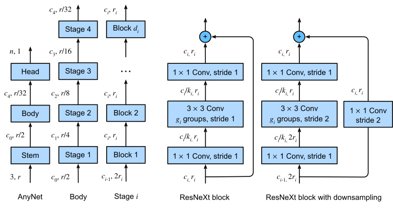
Let’s review the structure outlined in Fig. 8.8.1 in detail. As mentioned, an AnyNet consists of a stem, body, and head. The stem takes as its input RGB images (3 channels), using a 3×3 convolution with a stride of 2, followed by a batch norm, to halve the resolution from r×r to r/2×r/2. Moreover, it generates c0 channels that serve as input to the body.
그림 8.8.1의 구조를 자세히 살펴보자. 언급한 바와 같이 AnyNet은 스템, 바디, 헤드로 구성됩니다. 스템은 r×r에서 r/2×r/2로 해상도를 절반으로 줄이기 위해 스트라이드가 2인 3×3 컨볼루션을 사용하여 RGB 이미지(3개 채널)로 사용하고 배치 표준을 따릅니다. 또한 신체에 대한 입력 역할을 하는 c0 채널을 생성합니다.
Since the network is designed to work well with ImageNet images of shape 224×224×3, the body serves to reduce this to 7×7×c4 through 4 stages (recall that 224/21+4=7), each with an eventual stride of 2. Lastly, the head employs an entirely standard design via global average pooling, similar to NiN (Section 8.3), followed by a fully connected layer to emit an n-dimensional vector for n-class classification.
네트워크는 224×224×3 모양의 ImageNet 이미지와 잘 작동하도록 설계되었기 때문에 본문은 이를 4단계(224/2^1+4=7임을 상기)를 통해 7×7×c4로 줄이는 역할을 합니다. 마지막으로, 헤드는 NiN(섹션 8.3)과 유사한 전역 평균 풀링을 통해 완전히 표준적인 디자인을 사용하고, n-클래스 분류를 위해 n차원 벡터를 방출하기 위해 완전히 연결된 레이어가 뒤따릅니다.
Most of the relevant design decisions are inherent to the body of the network. It proceeds in stages, where each stage is composed of the same type of ResNeXt blocks as we discussed in Section 8.6.5. The design there is again entirely generic: we begin with a block that halves the resolution by using a stride of 2 (the rightmost in Fig. 8.8.1). To match this, the residual branch of the ResNeXt block needs to pass through a 1×1 convolution. This block is followed by a variable number of additional ResNeXt blocks that leave both resolution and the number of channels unchanged. Note that a common design practice is to add a slight bottleneck in the design of convolutional blocks. As such, with bottleneck ratio ki≥1 we afford some number of channels ci/ki within each block for stage i (as the experiments show, this is not really effective and should be skipped). Lastly, since we are dealing with ResNeXt blocks, we also need to pick the number of groups gi for grouped convolutions at stage i.
대부분의 관련 설계 결정은 네트워크 본문에 내재되어 있습니다. 각 단계는 섹션 8.6.5에서 논의한 것과 동일한 유형의 ResNeXt 블록으로 구성됩니다. 디자인은 다시 완전히 일반적입니다. 우리는 스트라이드 2(그림 8.8.1에서 가장 오른쪽)를 사용하여 해상도를 절반으로 줄이는 블록으로 시작합니다. 이를 일치시키려면 ResNeXt 블록의 잔여 분기가 1×1 컨벌루션을 통과해야 합니다. 이 블록 다음에는 해상도와 채널 수를 모두 변경하지 않고 그대로 두는 다양한 수의 추가 ResNeXt 블록이 옵니다. 일반적인 설계 관행은 컨볼루션 블록 설계에 약간의 병목 현상을 추가하는 것입니다. 이와 같이 병목 비율이 ki≥1인 경우 단계 i에 대해 각 블록 내에서 일정 수의 채널 ci/ki를 제공합니다(실험에서 알 수 있듯이 이것은 실제로 효과적이지 않으며 건너뛰어야 합니다). 마지막으로 ResNeXt 블록을 다루기 때문에 단계 i에서 그룹화된 컨볼루션에 대한 그룹 gi의 수를 선택해야 합니다.
This seemingly generic design space provides us nonetheless with many parameters: we can set the block width (number of channels) c0,…c4, the depth (number of blocks) per stage d1,…d4, the bottleneck ratios k1,…k4, and the group widths (numbers of groups) g1,…g4. In total this adds up to 17 parameters, resulting in an unreasonably large number of configurations that would warrant exploring. We need some tools to reduce this huge design space effectively. This is where the conceptual beauty of design spaces comes in. Before we do so, let’s implement the generic design first.
겉보기에 일반적인 이 설계 공간은 그럼에도 불구하고 많은 매개변수를 제공합니다. 블록 폭(채널 수) c0,…c4, 단계당 깊이(블록 수) d1,…d4, 병목 비율 k1,…k4, 및 그룹 폭(그룹의 수) g1,…g4. 전체적으로 이것은 최대 17개의 매개변수를 추가하므로 탐색을 보증할 수 있는 비합리적으로 많은 수의 구성이 생성됩니다. 이 거대한 디자인 공간을 효과적으로 줄이기 위한 몇 가지 도구가 필요합니다. 이것은 디자인 공간의 개념적 아름다움이 들어오는 곳입니다. 그렇게 하기 전에 먼저 일반적인 디자인을 구현합시다.
class AnyNet(d2l.Classifier):
    def stem(self, num_channels):
        return nn.Sequential(
            nn.LazyConv2d(num_channels, kernel_size=3, stride=2, padding=1),
            nn.LazyBatchNorm2d(), nn.ReLU())
Each stage consists of depth ResNeXt blocks, where num_channels specifies the block width. Note that the first block halves the height and width of input images.
각 단계는 깊이 ResNeXt 블록으로 구성되며 여기서 num_channels는 블록 너비를 지정합니다. 첫 번째 블록은 입력 이미지의 높이와 너비를 반으로 나눕니다.
@d2l.add_to_class(AnyNet)
def stage(self, depth, num_channels, groups, bot_mul):
    blk = []
    for i in range(depth):
        if i == 0:
            blk.append(d2l.ResNeXtBlock(num_channels, groups, bot_mul,
                use_1x1conv=True, strides=2))
        else:
            blk.append(d2l.ResNeXtBlock(num_channels, groups, bot_mul))
    return nn.Sequential(*blk)
Putting the network stem, body, and head together, we complete the implementation of AnyNet.
네트워크 스템, 바디, 헤드를 합치면 AnyNet 구현이 완료됩니다.
@d2l.add_to_class(AnyNet)
def __init__(self, arch, stem_channels, lr=0.1, num_classes=10):
    super(AnyNet, self).__init__()
    self.save_hyperparameters()
    self.net = nn.Sequential(self.stem(stem_channels))
    for i, s in enumerate(arch):
        self.net.add_module(f'stage{i+1}', self.stage(*s))
    self.net.add_module('head', nn.Sequential(
        nn.AdaptiveAvgPool2d((1, 1)), nn.Flatten(),
        nn.LazyLinear(num_classes)))
    self.net.apply(d2l.init_cnn)
8.8.2. Distributions and Parameters of Design Spaces
As just discussed in Section 8.8.1, parameters of a design space are hyperparameters of networks in that design space. Consider the problem of identifying good parameters in the AnyNet design space. We could try finding the single best parameter choice for a given amount of computation (e.g., FLOPs and compute time). If we allowed for even only two possible choices for each parameter, we would have to explore 2^17=131072 combinations to find the best solution. This is clearly infeasible due to its exorbitant cost. Even worse, we do not really learn anything from this exercise in terms of how one should design a network. Next time we add, say, an X-stage, or a shift operation, or similar, we would need to start from scratch. Even worse, due to the stochasticity in training (rounding, shuffling, bit errors), no two runs are likely to produce exactly the same results. A better strategy is to try to determine general guidelines of how the choices of parameters should be related. For instance, the bottleneck ratio, the number of channels, blocks, groups, or their change between layers should ideally be governed by a collection of simple rules. The approach in Radosavovic et al. (2019) relies on the following four assumptions:
섹션 8.8.1에서 설명한 것처럼 디자인 공간의 매개변수는 해당 디자인 공간에 있는 네트워크의 하이퍼 매개변수입니다. AnyNet 설계 공간에서 좋은 매개변수를 식별하는 문제를 고려하십시오. 주어진 계산량(예: FLOP 및 계산 시간)에 대해 단일 최상의 매개변수 선택을 찾으려고 시도할 수 있습니다. 각 매개변수에 대해 두 가지 가능한 선택만 허용하는 경우 최상의 솔루션을 찾기 위해 2^17=131072 조합을 탐색해야 합니다. 이것은 엄청난 비용 때문에 분명히 실행 불가능합니다. 설상가상으로 우리는 네트워크를 어떻게 설계해야 하는지에 대해 이 연습에서 실제로 아무것도 배우지 않습니다. 다음에 예를 들어 X-단계 또는 교대 작업 또는 이와 유사한 작업을 추가할 때는 처음부터 다시 시작해야 합니다. 설상가상으로 훈련의 확률성(반올림, 섞기, 비트 오류)으로 인해 두 번의 실행이 정확히 동일한 결과를 생성할 가능성이 없습니다. 더 나은 전략은 매개변수 선택이 어떻게 연관되어야 하는지에 대한 일반적인 지침을 결정하는 것입니다. 예를 들어, 병목 현상 비율, 채널, 블록, 그룹의 수 또는 계층 간의 변경은 이상적으로 간단한 규칙 모음에 의해 제어되어야 합니다. Radosavovic et al. (2019)은 다음 네 가지 가정에 의존합니다.
- We assume that general design principles actually exist, such that many networks satisfying these requirements should offer good performance. Consequently, identifying a distribution over networks can be a good strategy. In other words, we assume that there are many good needles in the haystack.
우리는 이러한 요구 사항을 충족하는 많은 네트워크가 좋은 성능을 제공해야 하는 일반적인 설계 원칙이 실제로 존재한다고 가정합니다. 결과적으로 네트워크를 통한 분포를 식별하는 것이 좋은 전략이 될 수 있습니다. 즉, 우리는 건초 더미에 좋은 바늘이 많이 있다고 가정합니다. - We need not train networks to convergence before we can assess whether a network is good. Instead, it is sufficient to use the intermediate results as reliable guidance for final accuracy. Using (approximate) proxies to optimize an objective is referred to as multi-fidelity optimization (Forrester et al., 2007). Consequently, design optimization is carried out, based on the accuracy achieved after only a few passes through the dataset, reducing the cost significantly.
네트워크가 양호한지 평가하기 전에 네트워크를 수렴하도록 교육할 필요는 없습니다. 대신 최종 정확도에 대한 신뢰할 수 있는 지침으로 중간 결과를 사용하는 것으로 충분합니다. 목표를 최적화하기 위해 (대략적인) 프록시를 사용하는 것을 다중 충실도 최적화라고 합니다(Forrester et al., 2007). 결과적으로 데이터 세트를 몇 번 통과한 후에 달성된 정확도를 기반으로 설계 최적화가 수행되어 비용이 크게 절감됩니다. - Results obtained at a smaller scale (for smaller networks) generalize to larger ones. Consequently, optimization is carried out for networks that are structurally similar, but with a smaller number of blocks, fewer channels, etc. Only in the end will we need to verify that the so-found networks also offer good performance at scale.
더 작은 규모(소규모 네트워크의 경우)에서 얻은 결과는 더 큰 규모로 일반화됩니다. 결과적으로 구조적으로 유사하지만 더 적은 수의 블록, 더 적은 채널 등을 가진 네트워크에 대해 최적화가 수행됩니다. 결국 우리는 이렇게 발견된 네트워크가 대규모로 우수한 성능을 제공하는지 확인해야 합니다. - Aspects of the design can be approximately factorized such that it is possible to infer their effect on the quality of the outcome somewhat independently. In other words, the optimization problem is moderately easy.
디자인의 측면은 결과의 품질에 대한 영향을 다소 독립적으로 추론할 수 있도록 대략적으로 분해될 수 있습니다. 즉, 최적화 문제는 적당히 쉽습니다.
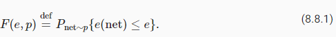
These assumptions allow us to test many networks cheaply. In particular, we can sample uniformly from the space of configurations and evaluate their performance. Subsequently, we can evaluate the quality of the choice of parameters by reviewing the distribution of error/accuracy that can be achieved with said networks. Denote by F(e) the cumulative distribution function (CDF) for errors committed by networks of a given design space, drawn using probability disribution p. That is,
이러한 가정을 통해 많은 네트워크를 저렴하게 테스트할 수 있습니다. 특히 구성 공간에서 균일하게 샘플링하여 성능을 평가할 수 있습니다. 그 후, 상기 네트워크로 달성할 수 있는 오류/정확도 분포를 검토하여 매개변수 선택의 품질을 평가할 수 있습니다. F(e)는 확률 분포 p를 사용하여 도출된 주어진 설계 공간의 네트워크에서 저지른 오류에 대한 누적 분포 함수(CDF)를 나타냅니다. 그건,
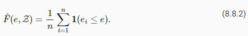
Our goal is now to find a distribution p over networks such that most networks have a very low error rate and where the support of p is concise. Of course, this is computationally infeasible to perform accurately. We resort to a sample of networks Z=def {net1,…netn} (with errors e1,…,en, respectively) from p and use the empirical CDF F^(e,Z) instead:
우리의 목표는 이제 대부분의 네트워크가 오류율이 매우 낮고 p의 지원이 간결한 네트워크를 통해 분포 p를 찾는 것입니다. 물론 이것은 정확하게 수행하기 위해 계산적으로 불가능합니다. 우리는 p에서 네트워크 Z=def {net1...netn}(각각 오류 e1,…,en 포함)의 샘플에 의존하고 대신 경험적 CDF F^(e,Z)를 사용합니다.
Whenever the CDF for one set of choices majorizes (or matches) another CDF it follows that its choice of parameters is superior (or indifferent). Accordingly Radosavovic et al. (2020) experimented with a shared network bottleneck ratio ki=k for all stages i of the network. This gets rid of 3 of the 4 parameters governing the bottleneck ratio. To assess whether this (negatively) affects the performance one can draw networks from the constrained and from the unconstrained distribution and compare the corresonding CDFs. It turns out that this constraint does not affect accuracy of the distribution of networks at all, as can be seen in the first panel of Fig. 8.8.2. Likewise, we could choose to pick the same group width gi=g occurring at the various stages of the network. Again, this does not affect performance, as can be seen in the second panel of Fig. 8.8.2. Both steps combined reduce the number of free parameters by 6.
하나의 선택 세트에 대한 CDF가 다른 CDF를 메이저화(또는 일치)할 때마다 매개변수 선택이 우월(또는 무관심)합니다. 따라서 Radosavovic et al. (2020)은 네트워크의 모든 단계 i에 대해 공유 네트워크 병목 현상 비율 ki=k로 실험했습니다. 이렇게 하면 병목 현상 비율을 제어하는 4개의 매개변수 중 3개가 제거됩니다. 이것이 성능에 (부정적인) 영향을 미치는지 평가하기 위해 제약이 있는 분포와 제약이 없는 분포에서 네트워크를 끌어와 해당 CDF를 비교할 수 있습니다. 그림 8.8.2의 첫 번째 패널에서 볼 수 있듯이 이 제약 조건은 네트워크 분포의 정확도에 전혀 영향을 미치지 않는 것으로 나타났습니다. 마찬가지로 네트워크의 다양한 단계에서 발생하는 동일한 그룹 너비 gi=g를 선택하도록 선택할 수 있습니다. 다시 말하지만 이것은 그림 8.8.2의 두 번째 패널에서 볼 수 있듯이 성능에 영향을 미치지 않습니다. 두 단계를 결합하면 사용 가능한 매개변수의 수가 6개 줄어듭니다.
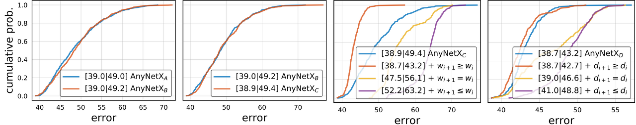
Next we look for ways to reduce the multitude of potential choices for width and depth of the stages. It is a reasonable assumption that as we go deeper, the number of channels should increase, i.e., ci≥ci−1 (wi+1≥wi per their notation in Fig. 8.8.2), yielding AnyNetXD. Likewise, it is equally reasonable to assume that as the stages progress, they should become deeper, i.e., di≥di−1, yielding AnyNetXE. This can be experimentally verified in the third and fourth panel of Fig. 8.8.2, respectively.
다음으로 스테이지의 폭과 깊이에 대한 다양한 잠재적 선택을 줄이는 방법을 찾습니다. 더 깊이 들어갈수록 채널 수가 증가해야 한다는 합리적인 가정입니다. 마찬가지로 단계가 진행됨에 따라 단계가 더 깊어져야 한다고 가정하는 것도 마찬가지로 합리적입니다(예: di≥di-1). 이는 그림 8.8.2의 세 번째와 네 번째 패널에서 각각 실험적으로 확인할 수 있다.
8.8.3. RegNet
The resulting AnyNetXE design space consists of simple networks following easy-to-interpret design principles:
결과적인 AnyNetXE 설계 공간은 해석하기 쉬운 설계 원칙을 따르는 간단한 네트워크로 구성됩니다.
- Share the bottleneck ratio ki=k for all stages i;
- Share the group width gi=g for all stages i;
- Increase network width across stages: ci≤ci+1;
- Increase network depth across stages: di≤di+1.
This leaves us with the last set of choices: how to pick the specific values for the above parameters of the eventual AnyNetXE design space. By studying the best-performing networks from the distribution in AnyNetXE one can observe that: the width of the network ideally increases linearly with the block index across the network, i.e., cj≈c0+caj, where j is the block index and slope ca>0. Given that we get to choose a different block width only per stage, we arrive at a piecewise constant function, engineered to match this dependence. Secondly, experiments also show that a bottleneck ratio of k=1 performs best, i.e., we are advised not to use bottlenecks at all.
최종적인 AnyNetXE 설계 공간의 위 매개변수에 대한 특정 값을 선택하는 방법과 같은 마지막 선택 세트가 남아 있습니다. AnyNetXE의 분포에서 가장 성능이 좋은 네트워크를 연구하면 다음을 관찰할 수 있습니다. 네트워크의 너비는 네트워크 전체의 블록 인덱스와 함께 이상적으로 선형적으로 증가합니다. 즉, cj≈c0+caj, 여기서 j는 블록 인덱스이고 기울기 ca >0. 단계마다 다른 블록 폭을 선택할 수 있다는 점을 감안할 때, 이 종속성과 일치하도록 설계된 조각별 상수 함수에 도달합니다. 둘째, 실험은 k=1의 병목 현상 비율이 가장 잘 수행됨을 보여줍니다. 즉, 병목 현상을 전혀 사용하지 않는 것이 좋습니다.
We recommend the interested reader to review further details for how to design specific networks for different amounts of computation by perusing Radosavovic et al. (2020). For instance, an effective 32-layer RegNetX variant is given by k=1 (no bottleneck), g=16 (group width is 16), c1=32 and c2=80 channels for the first and second stage, respectively, chosen to be d1=4 and d2=6 blocks deep. The astonishing insight from the design is that it applies, even when investigating networks at a larger scale. Even better, it even holds for Squeeze-and-Excitation (SE) network designs (RegNetY) that have a global channel activation (Hu et al., 2018).
관심 있는 독자는 Radosavovic et al. (2020). 예를 들어, 효과적인 32계층 RegNetX 변형은 k=1(병목 현상 없음), g=16(그룹 너비는 16), c1=32 및 c2=80 채널로 각각 첫 번째 및 두 번째 단계에 대해 선택됩니다. d1=4 및 d2=6 블록 깊이여야 합니다. 설계의 놀라운 통찰력은 더 큰 규모의 네트워크를 조사할 때에도 적용된다는 것입니다. 더 나아가 글로벌 채널 활성화가 있는 Squeeze-and-Excitation(SE) 네트워크 설계(RegNetY)에도 적용됩니다(Hu et al., 2018).
class RegNetX32(AnyNet):
    def __init__(self, lr=0.1, num_classes=10):
        stem_channels, groups, bot_mul = 32, 16, 1
        depths, channels = (4, 6), (32, 80)
        super().__init__(
            ((depths[0], channels[0], groups, bot_mul),
             (depths[1], channels[1], groups, bot_mul)),
            stem_channels, lr, num_classes)
We can see that each RegNetX stage progressively reduces resolution and increases output channels.
각 RegNetX 단계가 점진적으로 해상도를 줄이고 출력 채널을 증가시키는 것을 볼 수 있습니다.
RegNetX32().layer_summary((1, 1, 96, 96))Sequential output shape: torch.Size([1, 32, 48, 48])
Sequential output shape: torch.Size([1, 32, 24, 24])
Sequential output shape: torch.Size([1, 80, 12, 12])
Sequential output shape: torch.Size([1, 10])
8.8.4. Training
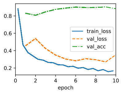
Training the 32-layer RegNetX on the Fashion-MNIST dataset is just like before.
Fashion-MNIST 데이터 세트에서 32계층 RegNetX를 교육하는 것은 이전과 동일합니다.
model = RegNetX32(lr=0.05)
trainer = d2l.Trainer(max_epochs=10, num_gpus=1)
data = d2l.FashionMNIST(batch_size=128, resize=(96, 96))
trainer.fit(model, data)
8.8.5. Discussion
With desirable inductive biases (assumptions or preferences) like locality and translation invariance (Section 7.1) for vision, CNNs have been the dominant architectures in this area. This has remained the case since LeNet up until recently when Transformers (Section 11.7) (Dosovitskiy et al., 2021, Touvron et al., 2021) started surpassing CNNs in terms of accuracy. While much of the recent progress in terms of vision Transformers can be backported into CNNs (Liu et al., 2022), it is only possible at a higher computational cost. Just as importantly, recent hardware optimizations (NVIDIA Ampere and Hopper) have only widened the gap in favor of Transformers.
시각에 대한 지역성 및 변환 불변성(섹션 7.1)과 같은 바람직한 귀납적 편향(가정 또는 선호도)을 통해 CNN은 이 영역에서 지배적인 아키텍처였습니다. 이는 트랜스포머(섹션 11.7)(Dosovitskiy et al., 2021, Touvron et al., 2021)가 정확성 측면에서 CNN을 능가하기 시작한 최근까지 LeNet 이후로 계속 유지되었습니다. 비전 트랜스포머 측면에서 최근의 많은 발전이 CNN으로 백포트될 수 있지만(Liu et al., 2022), 더 높은 계산 비용에서만 가능합니다. 마찬가지로 중요한 것은 최근의 하드웨어 최적화(NVIDIA Ampere 및 Hopper)가 트랜스포머에 유리한 격차를 더 벌렸을 뿐입니다.
It is worth noting that Transformers have a significantly lower degree of inductive bias towards locality and translation invariance than CNNs. It is not the least due to the availability of large image collections, such as LAION-400m and LAION-5B (Schuhmann et al., 2022) with up to 5 billion images that learned structures prevailed. Quite surprisingly, some of the more relevant work in this context even includes MLPs (Tolstikhin et al., 2021).
Transformers는 CNN보다 locality 및 translation invariance에 대한 귀납적 편향이 훨씬 낮다는 점은 주목할 가치가 있습니다. 학습 구조가 우세한 최대 50억 개의 이미지가 포함된 LAION-400m 및 LAION-5B(Schuhmann et al., 2022)와 같은 대규모 이미지 컬렉션의 가용성으로 인해 최소한이 아닙니다. 놀랍게도 이 맥락에서 더 관련성이 높은 일부 작업에는 MLP도 포함됩니다(Tolstikhin et al., 2021).
In sum, vision Transformers (Section 11.8) by now lead in terms of state-of-the-art performance in large-scale image classification, showing that scalability trumps inductive biases (Dosovitskiy et al., 2021). This includes pretraining large-scale Transformers (Section 11.9) with multi-head self-attention (Section 11.5). We invite the readers to dive into these chapters for a much more detailed discussion.
11.5. Multi-Head Attention — Dive into Deep Learning 1.0.0-beta0 documentation
d2l.ai
요약하면 비전 트랜스포머(섹션 11.8)는 이제 대규모 이미지 분류에서 최첨단 성능 측면에서 선두를 달리고 있으며 확장성이 유도 편향을 능가한다는 것을 보여줍니다(Dosovitskiy et al., 2021). 여기에는 multi-head self-attention(섹션 11.5)을 사용하여 대규모 Transformers(섹션 11.9)를 사전 훈련하는 것이 포함됩니다. 우리는 독자들이 훨씬 더 자세한 논의를 위해 이 장으로 뛰어들도록 초대합니다.
'Dive into Deep Learning > D2L Convolutional Neural Networks (CNN)' 카테고리의 다른 글
| D2L - 8.7. Densely Connected Networks (DenseNet) (0) | 2023.07.18 |
|---|---|
| D2L - 8.6. Residual Networks (ResNet) and ResNeXt (0) | 2023.07.18 |
| D2L - 8.5. Batch Normalization (0) | 2023.07.18 |
| D2L - 8.4. Multi-Branch Networks (GoogLeNet) (0) | 2023.07.18 |
| D2L - 8.3. Network in Network (NiN) (0) | 2023.07.11 |
| D2L - 8.2. Networks Using Blocks (VGG) (0) | 2023.07.10 |
| D2L - 8.1. Deep Convolutional Neural Networks (AlexNet) (0) | 2023.07.10 |
| D2L - 8. Modern Convolutional Neural Networks (0) | 2023.07.10 |
| D2L - 7.6. Convolutional Neural Networks (LeNet) (0) | 2023.07.09 |
| D2L - 7.5. Pooling (1) | 2023.07.09 |