

8.3. Network in Network (NiN) — Dive into Deep Learning 1.0.0-beta0 documentation (d2l.ai)
8.3. Network in Network (NiN) — Dive into Deep Learning 1.0.0-beta0 documentation
d2l.ai
8.3. Network in Network (NiN)
LeNet, AlexNet, and VGG all share a common design pattern: extract features exploiting spatial structure via a sequence of convolutions and pooling layers and post-process the representations via fully connected layers. The improvements upon LeNet by AlexNet and VGG mainly lie in how these later networks widen and deepen these two modules.
LeNet, AlexNet 및 VGG는 모두 공통 설계 패턴을 공유합니다. 컨볼루션 시퀀스 및 풀링 레이어를 통해 spatial 구조를 활용하는 기능을 추출하고 완전히 연결된 레이어를 통해 representations 을 후처리합니다. AlexNet 및 VGG에 의한 LeNet의 개선 사항은 주로 이러한 최신 네트워크가 이 두 모듈을 확장하고 심화시키는 방법에 있습니다.
This design poses two major challenges. First, the fully connected layers at the end of the architecture consume tremendous numbers of parameters. For instance, even a simple model such as VGG-11 requires a monstrous 25088×4096 matrix, occupying almost 400MB of RAM in single precision (FP32). This is a significant impediment to computation, in particular on mobile and embedded devices. After all, even high-end mobile phones sport no more than 8GB of RAM. At the time VGG was invented, this was an order of magnitude less (the iPhone 4S had 512MB). As such, it would have been difficult to justify spending the majority of memory on an image classifier.
이 설계에는 두 가지 주요 과제가 있습니다. 첫째, 아키텍처 끝에 있는 fully connected layers은 엄청난 수의 매개변수를 사용합니다. 예를 들어, VGG-11과 같은 간단한 모델도 단일 정밀도(FP32)에서 거의 400MB의 RAM을 차지하는 엄청난 25088×4096 매트릭스가 필요합니다. 이것은 특히 모바일 및 임베디드 장치에서 계산에 상당한 장애가 됩니다. 결국 고급 휴대폰도 8GB 이하의 RAM을 사용합니다. VGG가 발명되었을 때 이것은 훨씬 적었습니다(iPhone 4S는 512MB였습니다). 따라서 이미지 분류기에 대부분의 메모리를 소비하는 것을 정당화하기 어려웠을 것입니다.
Second, it is equally impossible to add fully connected layers earlier in the network to increase the degree of nonlinearity: doing so would destroy the spatial structure and require potentially even more memory.
둘째, 비선형성의 정도를 높이기 위해 네트워크 초기에 완전히 연결된 계층을 추가하는 것도 똑같이 불가능합니다. 그렇게 하면 공간 구조가 파괴되고 잠재적으로 더 많은 메모리가 필요할 수 있습니다.
The network in network (NiN) blocks (Lin et al., 2013) offer an alternative, capable of solving both problems in one simple strategy. They were proposed based on a very simple insight: (i) use 1×1 convolutions to add local nonlinearities across the channel activations and (ii) use global average pooling to integrate across all locations in the last representation layer. Note that global average pooling would not be effective, were it not for the added nonlinearities. Let’s dive into this in detail.
network in network (NiN) blocks (Lin et al., 2013)는 하나의 간단한 전략으로 두 가지 문제를 모두 해결할 수 있는 대안을 제공합니다. 그들은 매우 간단한 통찰력을 기반으로 제안되었습니다. (i) 1×1 컨볼루션을 사용하여 채널 활성화에 로컬 비선형성을 추가하고 (ii) global average pooling을 사용하여 마지막 representation 레이어의 모든 위치에 걸쳐 통합합니다. 추가된 비선형성이 없다면 전역 평균 풀링은 효과적이지 않을 것입니다. 이에 대해 자세히 알아보겠습니다.
Network in Network (NiN) 이란?
Network in Network (NiN) is a deep learning architecture introduced to enhance the expressiveness and efficiency of convolutional neural networks (CNNs). Unlike traditional CNNs that use linear filters followed by nonlinear activation functions, NiN introduces the concept of "micro neural networks" to capture complex patterns within each spatial location.
네트워크 인 네트워크(NiN)는 합성곱 신경망(Convolutional Neural Network, CNN)의 표현력과 효율성을 향상시키기 위해 도입된 딥러닝 아키텍처입니다. 기존의 CNN이 선형 필터를 사용하고 이후에 비선형 활성화 함수를 적용하는 방식과는 달리, NiN은 "마이크로 신경망"이라고 불리는 개념을 도입하여 각 공간 위치에서 복잡한 패턴을 포착합니다.
In NiN, instead of using a single convolutional layer with linear filters, it employs a set of parallel MLP-like convolutional layers called "networks". Each network consists of a series of 1x1 convolutional layers followed by nonlinearity. These 1x1 convolutions are responsible for capturing the nonlinear interactions between the channels. By stacking these network modules, NiN can learn more expressive feature representations.
NiN에서는 선형 필터로 구성된 단일 합성곱 레이어 대신 "네트워크"라고 불리는 병렬 MLP(다중 퍼셉트론) 형태의 합성곱 레이어 집합을 사용합니다. 각 네트워크는 1x1 합성곱 레이어들과 비선형 활성화 함수로 구성됩니다. 이러한 1x1 합성곱은 채널 간의 비선형 상호작용을 포착하는 역할을 담당합니다. 이러한 네트워크 모듈들을 쌓음으로써 NiN은 더욱 표현력 있는 특성 표현을 학습할 수 있습니다.
The key advantages of NiN are its ability to capture complex features using small receptive fields, reducing the number of parameters and improving computational efficiency. It also introduces a global average pooling layer that spatially averages the features to form a fixed-length vector, enabling the network to have a flexible input size.
NiN의 주요 장점은 작은 수용 영역을 사용하여 복잡한 특성을 포착할 수 있으며, 매개변수 수를 줄이고 계산 효율성을 향상시킬 수 있다는 것입니다. 또한, 입력 크기에 유연하게 대응할 수 있도록 전역 평균 풀링 레이어를 도입합니다.
NiN has been successful in various computer vision tasks, showing improved performance and interpretability compared to traditional CNN architectures.
NiN은 다양한 컴퓨터 비전 작업에서 성공적으로 적용되어 기존의 CNN 아키텍처와 비교하여 성능과 해석 가능성을 향상시킵니다.
Network In Network(NIN) 정리 (velog.io)
Network In Network(NIN) 정리
2014년에 ICLR에 accept된 Network In Network를 정리해본다.논문 작성자는 수용영역안에서 local patches에 대한 모델 차별성을 높이기 위해 Network In Network 모델 구조를 제시한다.고전적 convolution 모델은 비
velog.io
Micro Neural Network : 전통적 convolution 모델은 비선형 활성화 함수 + 선형 필터. but NiN은 수용 영역 안에서 데이터를 더 복잡하게 추상화 할 수 있는 micro neural network를 사용
Global average pooling : 모델 해석이 쉬워짐, fully-connected layer에서 발생할 수 있는 over-fitting 영향 줄여줌
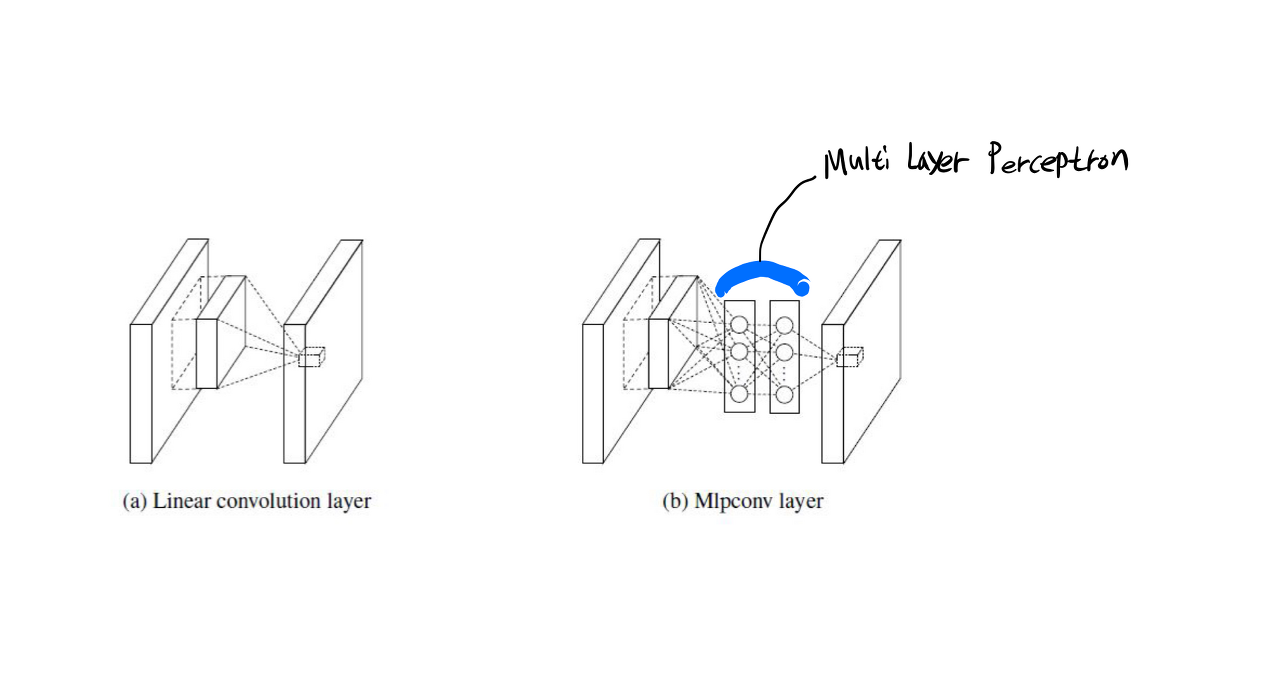
Mlpconv Layer를 여러겹 쌓은 것이 NiN임
NiN에서는 classification을 위해 fully connected layer대신 global average pooling을 사용.
fully connected layer는 dropout에 의존적이고 파라미터 수가 폭발적으로 증가
global average pooling은 파라미터 수가 늘지 않기 때문에 overfitting이 되지 않음
일반적인 CNN은 conv layer를 지난 feature map이 fully connected layer를 거친 후 softmax layer를 통해 결과 값 제시
NiN에서는 fully connected layer 대신 global average pooling을 제시
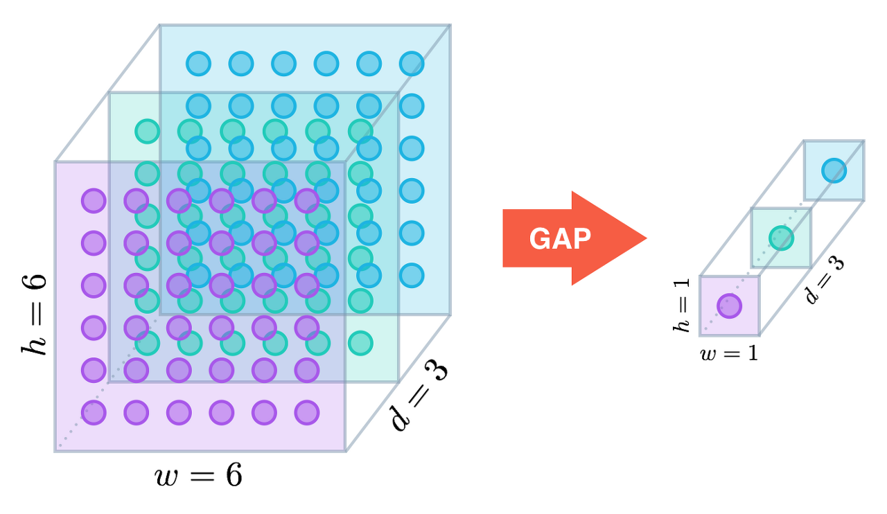
global average pooling은 이 그림에서 처럼 각 feature map의 평균을 계산하는 것.
conv layer를 통과한 각각의 feature map을 평균을 냄. 그러므로 각 feature map의 특성이 어느정도 남아 있다.
==> 이는 모델의 해석에 도움을 준다. 평균을 내기 때문에 parameter가 없다. (overfitting) 방지
NiN Structure
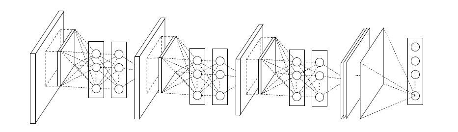
이 Structure에서는 3개의 Mlpconv layers와 global average pooling layer로 구성. (layer의 갯수는 변할 수 있다.)
import torch
from torch import nn
from d2l import torch as d2l
8.3.1. NiN Blocks
Recall Section 7.4.3. In it we discussed that the inputs and outputs of convolutional layers consist of four-dimensional tensors with axes corresponding to the example, channel, height, and width. Also recall that the inputs and outputs of fully connected layers are typically two-dimensional tensors corresponding to the example and feature. The idea behind NiN is to apply a fully connected layer at each pixel location (for each height and width). The resulting 1×1 convolution can be thought as a fully connected layer acting independently on each pixel location.
섹션 7.4.3을 상기하십시오. 여기에서 우리는 컨볼루션 레이어의 입력과 출력이 채널, 높이 및 너비에 해당하는 축을 가진 4차원 텐서로 구성된다고 논의했습니다. 또한 완전히 연결된 계층의 입력과 출력은 일반적으로 예제와 기능에 해당하는 2차원 텐서라는 점을 상기하십시오. NiN의 기본 아이디어는 각 픽셀 위치(각 높이와 너비에 대해)에 완전히 연결된 레이어를 적용하는 것입니다. 결과 1×1 컨볼루션은 각 픽셀 위치에서 독립적으로 작동하는 완전히 연결된 레이어로 생각할 수 있습니다.
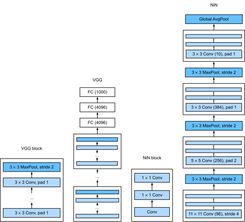
Fig. 8.3.1 illustrates the main structural differences between VGG and NiN, and their blocks. Note both the difference in the NiN blocks (the initial convolution is followed by 1×1 convolutions, whereas VGG retains 3×3 convolutions) and in the end where we no longer require a giant fully connected layer.
그림 8.3.1은 VGG와 NiN 사이의 주요 구조적 차이점과 해당 블록을 보여줍니다. NiN 블록의 차이점(초기 컨볼루션 다음에는 1×1 컨볼루션이 이어지는 반면 VGG는 3×3 컨볼루션을 유지함)과 결국 더 이상 거대한 fully connected layer가 필요하지 않은 점에 유의하십시오.
def nin_block(out_channels, kernel_size, strides, padding):
    return nn.Sequential(
        nn.LazyConv2d(out_channels, kernel_size, strides, padding), nn.ReLU(),
        nn.LazyConv2d(out_channels, kernel_size=1), nn.ReLU(),
nn.LazyConv2d(out_channels, kernel_size=1), nn.ReLU())- nin_block 함수는 NiN 블록을 생성하는 함수입니다. 이 함수는 출력 채널 수 out_channels, 커널 크기 kernel_size, 스트라이드 strides, 패딩 padding을 인자로 받습니다.
- nn.Sequential은 여러 개의 모듈을 순차적으로 쌓아 하나의 모듈로 만들어주는 함수입니다. 이를 통해 NiN 블록을 정의합니다.
- 첫 번째 nn.LazyConv2d 레이어는 출력 채널 수 out_channels, 커널 크기 kernel_size, 스트라이드 strides, 패딩 padding을 가진 합성곱 레이어입니다. 이후에 nn.ReLU() 함수를 사용하여 비선형 활성화 함수인 ReLU를 적용합니다.
- 두 번째와 세 번째 nn.LazyConv2d 레이어는 출력 채널 수 out_channels, 커널 크기 1을 가진 합성곱 레이어입니다. 이는 NiN 블록 내에서 1x1 컨볼루션 연산을 수행하기 위한 레이어입니다. 마찬가지로 nn.ReLU() 함수를 사용하여 비선형 활성화 함수인 ReLU를 적용합니다.
- 이렇게 생성된 레이어들은 nn.Sequential을 통해 하나의 모듈로 합쳐진 후 반환됩니다.
8.3.2. NiN Model
NiN uses the same initial convolution sizes as AlexNet (it was proposed shortly thereafter). The kernel sizes are 11×11, 5×5, and 3×3, respectively, and the numbers of output channels match those of AlexNet. Each NiN block is followed by a max-pooling layer with a stride of 2 and a window shape of 3×3.
NiN은 AlexNet과 동일한 초기 컨볼루션 크기를 사용합니다(그 직후에 제안됨). 커널 크기는 각각 11×11, 5×5, 3×3이며 출력 채널의 수는 AlexNet과 일치합니다. 각 NiN 블록 다음에는 보폭이 2이고 창 모양이 3×3인 최대 풀링 레이어가 옵니다.
The second significant difference between NiN and both AlexNet and VGG is that NiN avoids fully connected layers altogether. Instead, NiN uses a NiN block with a number of output channels equal to the number of label classes, followed by a global average pooling layer, yielding a vector of logits. This design significantly reduces the number of required model parameters, albeit at the expense of a potential increase in training time.
NiN과 AlexNet 및 VGG의 두 번째 중요한 차이점은 NiN이 fully connected layers를 모두 피한다는 것입니다. 대신 NiN은 레이블 클래스 수와 동일한 수의 출력 채널이 있는 NiN 블록을 사용하고 뒤이어 global average pooling layer 를 사용하여 로짓 벡터를 생성합니다. 이 디자인은 학습 시간이 잠재적으로 증가하더라도 필요한 모델 매개변수의 수를 크게 줄입니다.
class NiN(d2l.Classifier):
    def __init__(self, lr=0.1, num_classes=10):
        super().__init__()
        self.save_hyperparameters()
        self.net = nn.Sequential(
            nin_block(96, kernel_size=11, strides=4, padding=0),
            nn.MaxPool2d(3, stride=2),
            nin_block(256, kernel_size=5, strides=1, padding=2),
            nn.MaxPool2d(3, stride=2),
            nin_block(384, kernel_size=3, strides=1, padding=1),
            nn.MaxPool2d(3, stride=2),
            nn.Dropout(0.5),
            nin_block(num_classes, kernel_size=3, strides=1, padding=1),
            nn.AdaptiveAvgPool2d((1, 1)),
            nn.Flatten())
self.net.apply(d2l.init_cnn)- NiN 클래스는 NiN 모델을 정의하는 클래스입니다. 생성자 함수 __init__을 통해 모델을 초기화합니다. 학습률 lr과 클래스의 개수 num_classes를 인자로 받습니다.
- super().__init__()을 사용하여 상위 클래스인 d2l.Classifier의 초기화 함수를 호출합니다.
- self.save_hyperparameters()를 사용하여 하이퍼파라미터를 저장합니다.
- self.net은 nn.Sequential을 통해 여러 개의 레이어를 순차적으로 쌓은 네트워크 모델입니다.
- nin_block 함수를 사용하여 NiN 블록을 생성하고 nn.Sequential에 추가합니다. 첫 번째 NiN 블록은 96개의 출력 채널을 가지며, 커널 크기는 11, 스트라이드는 4, 패딩은 0입니다.
- nn.MaxPool2d 레이어를 사용하여 최대 풀링을 수행합니다. 첫 번째 풀링 레이어는 커널 크기가 3이고 스트라이드가 2입니다.
- 두 번째 NiN 블록은 256개의 출력 채널을 가지며, 커널 크기는 5, 스트라이드는 1, 패딩은 2입니다.
- 두 번째 풀링 레이어는 동일하게 커널 크기가 3이고 스트라이드가 2입니다.
- 세 번째 NiN 블록은 384개의 출력 채널을 가지며, 커널 크기는 3, 스트라이드는 1, 패딩은 1입니다.
- 세 번째 풀링 레이어도 동일하게 커널 크기가 3이고 스트라이드가 2입니다.
- nn.Dropout 레이어를 사용하여 드롭아웃을 수행합니다. 확률은 0.5로 설정됩니다.
- 네 번째 NiN 블록은 클래스 개수 num_classes를 가지며, 커널 크기는 3, 스트라이드는 1, 패딩은 1입니다.
- nn.AdaptiveAvgPool2d 레이어를 사용하여 출력 특성맵의 크기를 고정된 크기로 조정합니다. 이 경우 (1, 1) 크기로 조정됩니다.
- nn.Flatten 레이어를 사용하여 특성맵을 1차원으로 평탄화합니다.
- self.net.apply(d2l.init_cnn)를 통해 네트워크의 가중치를 초기화합니다.
AdaptiveAvgPool2d — PyTorch 2.0 documentation
AdaptiveAvgPool2d — PyTorch 2.0 documentation
Shortcuts
pytorch.org
We create a data example to see the output shape of each block.
각 블록의 출력 형태를 보기 위해 데이터 예제를 생성합니다.
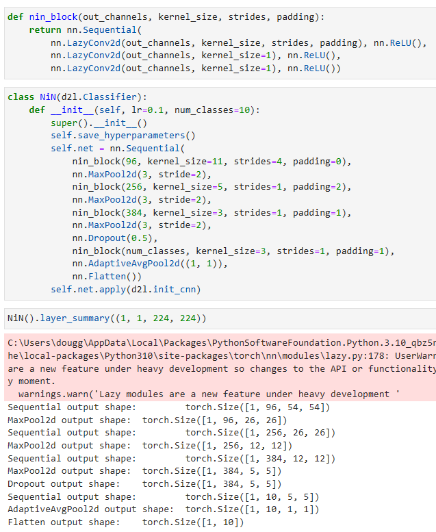
NiN().layer_summary((1, 1, 224, 224))- NiN 클래스의 인스턴스를 생성합니다.
- layer_summary 메서드를 호출하여 모델의 레이어 요약 정보를 출력합니다. 인자로 입력 데이터의 크기를 전달합니다. 이 경우 입력 데이터의 크기는 (1, 1, 224, 224)입니다.
8.3.3. Training
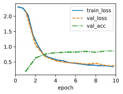
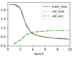
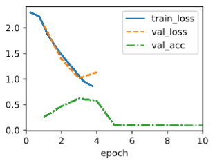
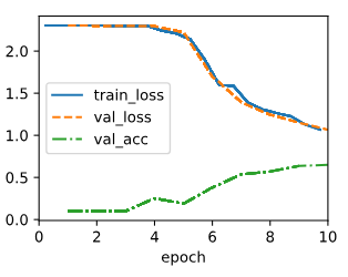
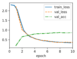
As before we use Fashion-MNIST to train the model using the same optimizer that we used for AlexNet and VGG.
이전과 마찬가지로 Fashion-MNIST를 사용하여 AlexNet 및 VGG에 사용한 것과 동일한 옵티마이저를 사용하여 모델을 교육합니다.
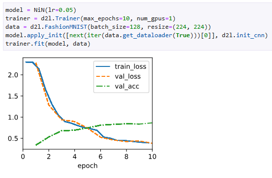
model = NiN(lr=0.05)
trainer = d2l.Trainer(max_epochs=10, num_gpus=1)
data = d2l.FashionMNIST(batch_size=128, resize=(224, 224))
model.apply_init([next(iter(data.get_dataloader(True)))[0]], d2l.init_cnn)
trainer.fit(model, data)- NiN 클래스의 인스턴스인 model을 생성합니다. 학습률 lr은 0.05로 설정되어 있습니다.
- Trainer 클래스의 인스턴스인 trainer를 생성합니다. max_epochs는 10으로 설정되어 있고, num_gpus는 1로 설정되어 있습니다.
- FashionMNIST 데이터셋을 로드합니다. 배치 크기는 128이고, 이미지 크기는 (224, 224)로 변경되도록 설정되어 있습니다.
- data를 사용하여 모델의 가중치를 초기화합니다. 초기화 방법은 d2l.init_cnn 함수를 사용하여 첫 번째 미니 배치의 입력 데이터로 초기화됩니다.
- trainer를 사용하여 model을 data에 대해 학습시킵니다.
SageMaker
CoLab
8.3.4. Summary
NiN has dramatically fewer parameters than AlexNet and VGG. This stems primarily from the fact that it needs no giant fully connected layers. Instead, it uses global average pooling to aggregate across all image locations after the last stage of the network body. This obviates the need for expensive (learned) reduction operations and replaces them by a simple average. What was surprising at the time is the fact that this averaging operation did not harm accuracy. Note that averaging across a low-resolution representation (with many channels) also adds to the amount of translation invariance that the network can handle.
NiN은 AlexNet 및 VGG보다 매개변수가 훨씬 적습니다. 이것은 주로 거대한 fully connected layers가 필요하지 않다는 사실에서 비롯됩니다. 대신 global average pooling을 사용하여 네트워크 본문의 마지막 단계 이후 모든 이미지 위치에 걸쳐 집계합니다. 이는 비용이 많이 드는(학습된) 축소 작업의 필요성을 없애고 단순 평균으로 대체합니다. 당시 놀라운 점은 이 평균 연산이 정확도를 해치지 않았다는 사실입니다. 저해상도 표현(많은 채널 포함)에 대한 평균화는 네트워크가 처리할 수 있는 변환 불변의 양을 추가합니다.
Choosing fewer convolutions with wide kernels and replacing them by 1×1 convolutions aids the quest for fewer parameters further. It affords for a significant amount of nonlinearity across channels within any given location. Both 1×1 convolutions and global average pooling significantly influenced subsequent CNN designs.
넓은 커널이 있는 더 적은 컨볼루션을 선택하고 1×1 컨볼루션으로 대체하면 더 적은 매개변수를 찾는 데 도움이 됩니다. 주어진 위치 내에서 채널 전반에 걸쳐 상당한 양의 비선형성을 제공합니다. 1×1 컨볼루션과 전역 평균 풀링은 후속 CNN 설계에 상당한 영향을 미쳤습니다.
8.3.5. Exercises
- Why are there two 1×1 convolutional layers per NiN block? Increase their number to three. Reduce their number to one. What changes?
- What changes if you replace the 1×1 convolutions by 3×3 convolutions?
- What happens if you replace the global average pooling by a fully connected layer (speed, accuracy, number of parameters)?
- Calculate the resource usage for NiN.
- What is the number of parameters?
- What is the amount of computation?
- What is the amount of memory needed during training?
- What is the amount of memory needed during prediction?
- What are possible problems with reducing the 384×5×5 representation to a 10×5×5 representation in one step?
- Use the structural design decisions in VGG that led to VGG-11, VGG-16, and VGG-19 to design a family of NiN-like networks.
'Dive into Deep Learning > D2L Convolutional Neural Networks (CNN)' 카테고리의 다른 글
| D2L - 8.8. Designing Convolution Network Architectures (0) | 2023.07.18 |
|---|---|
| D2L - 8.7. Densely Connected Networks (DenseNet) (0) | 2023.07.18 |
| D2L - 8.6. Residual Networks (ResNet) and ResNeXt (0) | 2023.07.18 |
| D2L - 8.5. Batch Normalization (0) | 2023.07.18 |
| D2L - 8.4. Multi-Branch Networks (GoogLeNet) (0) | 2023.07.18 |
| D2L - 8.2. Networks Using Blocks (VGG) (0) | 2023.07.10 |
| D2L - 8.1. Deep Convolutional Neural Networks (AlexNet) (0) | 2023.07.10 |
| D2L - 8. Modern Convolutional Neural Networks (0) | 2023.07.10 |
| D2L - 7.6. Convolutional Neural Networks (LeNet) (0) | 2023.07.09 |
| D2L - 7.5. Pooling (1) | 2023.07.09 |