

https://d2l.ai/chapter_convolutional-modern/densenet.html
8.7. Densely Connected Networks (DenseNet) — Dive into Deep Learning 1.0.0-beta0 documentation
d2l.ai
8.7. Densely Connected Networks (DenseNet)
ResNet significantly changed the view of how to parametrize the functions in deep networks. DenseNet (dense convolutional network) is to some extent the logical extension of this (Huang et al., 2017). DenseNet is characterized by both the connectivity pattern where each layer connects to all the preceding layers and the concatenation operation (rather than the addition operator in ResNet) to preserve and reuse features from earlier layers. To understand how to arrive at it, let’s take a small detour to mathematics.
ResNet은 심층 네트워크에서 기능을 매개변수화하는 방법에 대한 관점을 크게 변경했습니다. DenseNet(dense convolutional network)은 어느 정도 이것의 논리적 확장입니다(Huang et al., 2017). DenseNet은 각 레이어가 모든 이전 레이어에 연결되는 연결 패턴과 이전 레이어의 기능을 보존하고 재사용하기 위한 연결 작업(ResNet의 추가 연산자가 아님)이 모두 특징입니다. 그것에 도달하는 방법을 이해하기 위해 수학으로 약간 우회해 봅시다.
import torch
from torch import nn
from d2l import torch as d2l
8.7.1. From ResNet to DenseNet
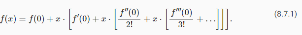
Recall the Taylor expansion for functions. For the point x=0 it can be written as
함수에 대한 Taylor 확장을 상기하십시오. 점 x=0에 대해 다음과 같이 쓸 수 있습니다.
The key point is that it decomposes a function into increasingly higher order terms. In a similar vein, ResNet decomposes functions into
요점은 함수를 점점 더 고차 항으로 분해한다는 것입니다. 유사한 맥락에서 ResNet은 기능을 다음으로 분해합니다.

That is, ResNet decomposes f into a simple linear term and a more complex nonlinear one. What if we wanted to capture (not necessarily add) information beyond two terms? One such solution is DenseNet (Huang et al., 2017).
즉, ResNet은 f를 간단한 선형 항과 더 복잡한 비선형 항으로 분해합니다. 두 용어 이상의 정보를 캡처(반드시 추가할 필요는 없음)하려면 어떻게 해야 합니까? 그러한 솔루션 중 하나가 DenseNet입니다(Huang et al., 2017).

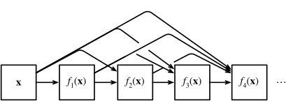
As shown in Fig. 8.7.1, the key difference between ResNet and DenseNet is that in the latter case outputs are concatenated (denoted by [,]) rather than added. As a result, we perform a mapping from x to its values after applying an increasingly complex sequence of functions:
그림 8.7.1에서 볼 수 있듯이 ResNet과 DenseNet의 주요 차이점은 후자의 경우 출력이 추가되지 않고 연결된다는 것입니다([,]로 표시). 결과적으로 점점 더 복잡한 함수 시퀀스를 적용한 후 x에서 해당 값으로 매핑을 수행합니다.

In the end, all these functions are combined in MLP to reduce the number of features again. In terms of implementation this is quite simple: rather than adding terms, we concatenate them. The name DenseNet arises from the fact that the dependency graph between variables becomes quite dense. The last layer of such a chain is densely connected to all previous layers. The dense connections are shown in Fig. 8.7.2.
결국 이러한 기능을 모두 MLP로 결합하여 기능 수를 다시 줄입니다. 구현 측면에서 이것은 매우 간단합니다. 용어를 추가하는 대신 용어를 연결합니다. DenseNet이라는 이름은 변수 간의 종속성 그래프가 상당히 조밀해진다는 사실에서 유래되었습니다. 이러한 체인의 마지막 레이어는 이전의 모든 레이어와 조밀하게 연결됩니다. 조밀한 연결은 그림 8.7.2에 나와 있습니다.
The main components that compose a DenseNet are dense blocks and transition layers. The former define how the inputs and outputs are concatenated, while the latter control the number of channels so that it is not too large, since the expansion x→[x,f1(x),f2([x,f1(x)]),…] can be quite high-dimensional.
DenseNet을 구성하는 주요 구성 요소는 dense block과 transition layer입니다. 전자는 입력과 출력이 연결되는 방식을 정의하고 후자는 너무 크지 않도록 채널 수를 제어합니다. 확장 x→[x,f1(x),f2([x,f1(x)] ),…]은 상당히 고차원적일 수 있습니다.
8.7.2. Dense Blocks
DenseNet uses the modified “batch normalization, activation, and convolution” structure of ResNet (see the exercise in Section 8.6). First, we implement this convolution block structure.
DenseNet은 ResNet의 수정된 "배치 정규화, 활성화 및 컨볼루션" 구조를 사용합니다(섹션 8.6의 실습 참조). 먼저 이 컨볼루션 블록 구조를 구현합니다.
def conv_block(num_channels):
    return nn.Sequential(
        nn.LazyBatchNorm2d(), nn.ReLU(),
        nn.LazyConv2d(num_channels, kernel_size=3, padding=1))
A dense block consists of multiple convolution blocks, each using the same number of output channels. In the forward propagation, however, we concatenate the input and output of each convolution block on the channel dimension. Lazy evaluation allows us to adjust the dimensionality automatically.
고밀도 블록은 각각 동일한 수의 출력 채널을 사용하는 여러 컨볼루션 블록으로 구성됩니다. 그러나 정방향 전파에서는 채널 차원에서 각 컨볼루션 블록의 입력과 출력을 연결합니다. 게으른 평가를 통해 차원을 자동으로 조정할 수 있습니다.
class DenseBlock(nn.Module):
    def __init__(self, num_convs, num_channels):
        super(DenseBlock, self).__init__()
        layer = []
        for i in range(num_convs):
            layer.append(conv_block(num_channels))
        self.net = nn.Sequential(*layer)

    def forward(self, X):
        for blk in self.net:
            Y = blk(X)
            # Concatenate input and output of each block along the channels
            X = torch.cat((X, Y), dim=1)
        return X
In the following example, we define a DenseBlock instance with 2 convolution blocks of 10 output channels. When using an input with 3 channels, we will get an output with 3+10+10=23 channels. The number of convolution block channels controls the growth in the number of output channels relative to the number of input channels. This is also referred to as the growth rate.
다음 예제에서는 10개 출력 채널의 2개 컨볼루션 블록으로 DenseBlock 인스턴스를 정의합니다. 3채널 입력을 사용하면 3+10+10=23채널 출력이 됩니다. 컨볼루션 블록 채널의 수는 입력 채널 수에 비해 출력 채널 수의 증가를 제어합니다. 이를 성장률이라고도 합니다.
blk = DenseBlock(2, 10)
X = torch.randn(4, 3, 8, 8)
Y = blk(X)
Y.shape
torch.Size([4, 23, 8, 8])
8.7.3. Transition Layers
Since each dense block will increase the number of channels, adding too many of them will lead to an excessively complex model. A transition layer is used to control the complexity of the model. It reduces the number of channels by using an 1×1 convolution. Moreover, it halves the height and width via average pooling with a stride of 2.
밀도가 높은 각 블록은 채널 수를 증가시키므로 채널을 너무 많이 추가하면 모델이 지나치게 복잡해집니다. 전환 레이어는 모델의 복잡성을 제어하는 데 사용됩니다. 1×1 컨벌루션을 사용하여 채널 수를 줄입니다. 또한 스트라이드 2의 평균 풀링을 통해 높이와 너비를 절반으로 줄입니다.
def transition_block(num_channels):
    return nn.Sequential(
        nn.LazyBatchNorm2d(), nn.ReLU(),
        nn.LazyConv2d(num_channels, kernel_size=1),
        nn.AvgPool2d(kernel_size=2, stride=2))
Apply a transition layer with 10 channels to the output of the dense block in the previous example. This reduces the number of output channels to 10, and halves the height and width.
이전 예에서 고밀도 블록의 출력에 10개의 채널이 있는 전환 레이어를 적용합니다. 이렇게 하면 출력 채널 수가 10개로 줄어들고 높이와 너비가 절반으로 줄어듭니다.
blk = transition_block(10)
blk(Y).shape
torch.Size([4, 10, 4, 4])
8.7.4. DenseNet Model
Next, we will construct a DenseNet model. DenseNet first uses the same single convolutional layer and max-pooling layer as in ResNet.
다음으로 DenseNet 모델을 구성합니다. DenseNet은 먼저 ResNet에서와 동일한 단일 컨벌루션 레이어와 최대 풀링 레이어를 사용합니다.
class DenseNet(d2l.Classifier):
    def b1(self):
        return nn.Sequential(
            nn.LazyConv2d(64, kernel_size=7, stride=2, padding=3),
            nn.LazyBatchNorm2d(), nn.ReLU(),
            nn.MaxPool2d(kernel_size=3, stride=2, padding=1))
Then, similar to the four modules made up of residual blocks that ResNet uses, DenseNet uses four dense blocks. Similar to ResNet, we can set the number of convolutional layers used in each dense block. Here, we set it to 4, consistent with the ResNet-18 model in Section 8.6. Furthermore, we set the number of channels (i.e., growth rate) for the convolutional layers in the dense block to 32, so 128 channels will be added to each dense block.
그런 다음 ResNet이 사용하는 잔차 블록으로 구성된 4개의 모듈과 유사하게 DenseNet은 4개의 고밀도 블록을 사용합니다. ResNet과 유사하게 각 고밀도 블록에서 사용되는 컨볼루션 레이어의 수를 설정할 수 있습니다. 여기에서는 섹션 8.6의 ResNet-18 모델과 일치하도록 4로 설정했습니다. 또한 dense 블록의 컨볼루션 레이어에 대한 채널 수(즉, 성장 속도)를 32로 설정하여 각 dense 블록에 128개의 채널을 추가합니다.
In ResNet, the height and width are reduced between each module by a residual block with a stride of 2. Here, we use the transition layer to halve the height and width and halve the number of channels. Similar to ResNet, a global pooling layer and a fully connected layer are connected at the end to produce the output.
ResNet에서 높이와 너비는 stride가 2인 잔여 블록에 의해 각 모듈 사이에서 줄어듭니다. 여기에서 전환 레이어를 사용하여 높이와 너비를 절반으로 줄이고 채널 수를 절반으로 줄입니다. ResNet과 유사하게 전역 풀링 계층과 완전히 연결된 계층이 끝에 연결되어 출력을 생성합니다.
@d2l.add_to_class(DenseNet)
def __init__(self, num_channels=64, growth_rate=32, arch=(4, 4, 4, 4),
             lr=0.1, num_classes=10):
    super(DenseNet, self).__init__()
    self.save_hyperparameters()
    self.net = nn.Sequential(self.b1())
    for i, num_convs in enumerate(arch):
        self.net.add_module(f'dense_blk{i+1}', DenseBlock(num_convs,
                                                          growth_rate))
        # The number of output channels in the previous dense block
        num_channels += num_convs * growth_rate
        # A transition layer that halves the number of channels is added
        # between the dense blocks
        if i != len(arch) - 1:
            num_channels //= 2
            self.net.add_module(f'tran_blk{i+1}', transition_block(
                num_channels))
    self.net.add_module('last', nn.Sequential(
        nn.LazyBatchNorm2d(), nn.ReLU(),
        nn.AdaptiveAvgPool2d((1, 1)), nn.Flatten(),
        nn.LazyLinear(num_classes)))
    self.net.apply(d2l.init_cnn)
8.7.5. Training
Since we are using a deeper network here, in this section, we will reduce the input height and width from 224 to 96 to simplify the computation.
여기에서 더 깊은 네트워크를 사용하고 있으므로 이 섹션에서는 계산을 단순화하기 위해 입력 높이와 너비를 224에서 96으로 줄입니다.
model = DenseNet(lr=0.01)
trainer = d2l.Trainer(max_epochs=10, num_gpus=1)
data = d2l.FashionMNIST(batch_size=128, resize=(96, 96))
trainer.fit(model, data)
8.7.6. Summary and Discussion
The main components that compose DenseNet are dense blocks and transition layers. For the latter, we need to keep the dimensionality under control when composing the network by adding transition layers that shrink the number of channels again. In terms of cross-layer connections, unlike ResNet, where inputs and outputs are added together, DenseNet concatenates inputs and outputs on the channel dimension. Although these concatenation operations reuse features to achieve computational efficiency, unfortunately they lead to heavy GPU memory consumption. As a result, applying DenseNet may require more memory-efficient implementations that may increase training time (Pleiss et al., 2017).
DenseNet을 구성하는 주요 구성 요소는 dense block과 transition layer입니다. 후자의 경우 채널 수를 다시 줄이는 전환 레이어를 추가하여 네트워크를 구성할 때 차원을 제어해야 합니다. 교차 계층 연결 측면에서 입력과 출력이 함께 추가되는 ResNet과 달리 DenseNet은 채널 차원에서 입력과 출력을 연결합니다. 이러한 연결 작업은 계산 효율성을 달성하기 위해 기능을 재사용하지만 불행하게도 GPU 메모리 사용량이 많이 발생합니다. 결과적으로 DenseNet을 적용하려면 훈련 시간을 늘릴 수 있는 메모리 효율적인 구현이 필요할 수 있습니다(Pleiss et al., 2017).
8.7.7. Exercises
- Why do we use average pooling rather than max-pooling in the transition layer?
- One of the advantages mentioned in the DenseNet paper is that its model parameters are smaller than those of ResNet. Why is this the case?
- One problem for which DenseNet has been criticized is its high memory consumption.
- Is this really the case? Try to change the input shape to 224×224 to see the actual GPU memory consumption empirically.
- Can you think of an alternative means of reducing the memory consumption? How would you need to change the framework?
- Implement the various DenseNet versions presented in Table 1 of the DenseNet paper (Huang et al., 2017).
- Design an MLP-based model by applying the DenseNet idea. Apply it to the housing price prediction task in Section 5.7.
'Dive into Deep Learning > D2L Convolutional Neural Networks (CNN)' 카테고리의 다른 글
| D2L - 8.8. Designing Convolution Network Architectures (0) | 2023.07.18 |
|---|---|
| D2L - 8.6. Residual Networks (ResNet) and ResNeXt (0) | 2023.07.18 |
| D2L - 8.5. Batch Normalization (0) | 2023.07.18 |
| D2L - 8.4. Multi-Branch Networks (GoogLeNet) (0) | 2023.07.18 |
| D2L - 8.3. Network in Network (NiN) (0) | 2023.07.11 |
| D2L - 8.2. Networks Using Blocks (VGG) (0) | 2023.07.10 |
| D2L - 8.1. Deep Convolutional Neural Networks (AlexNet) (0) | 2023.07.10 |
| D2L - 8. Modern Convolutional Neural Networks (0) | 2023.07.10 |
| D2L - 7.6. Convolutional Neural Networks (LeNet) (0) | 2023.07.09 |
| D2L - 7.5. Pooling (1) | 2023.07.09 |