

https://d2l.ai/chapter_attention-mechanisms-and-transformers/transformer.html
11.7. The Transformer Architecture — Dive into Deep Learning 1.0.0-beta0 documentation
d2l.ai
11.7. The Transformer Architecture
We have compared CNNs, RNNs, and self-attention in Section 11.6.2. Notably, self-attention enjoys both parallel computation and the shortest maximum path length. Therefore naturally, it is appealing to design deep architectures by using self-attention. Unlike earlier self-attention models that still rely on RNNs for input representations (Cheng et al., 2016, Lin et al., 2017, Paulus et al., 2017), the Transformer model is solely based on attention mechanisms without any convolutional or recurrent layer (Vaswani et al., 2017). Though originally proposed for sequence to sequence learning on text data, Transformers have been pervasive in a wide range of modern deep learning applications, such as in areas of language, vision, speech, and reinforcement learning.
섹션 11.6.2에서 CNN, RNN 및 self-attention을 비교했습니다. 특히 self-attention은 병렬 계산과 가장 짧은 최대 경로 길이를 모두 즐깁니다. 따라서 당연히 self-attention을 사용하여 심층적인 아키텍처를 설계하는 것이 매력적입니다. 입력 representations 에 대해 여전히 RNN에 의존하는 이전의 self-attention 모델(Cheng et al., 2016, Lin et al., 2017, Paulus et al., 2017)과 달리 Transformer 모델은 컨볼루션 또는 recurrent layer(Vaswani et al., 2017)에 없이 attention 메카니즘만을 사용합니다. 원래 텍스트 데이터에 대한 sequence to sequence learning을 위해 제안되었지만 트랜스포머는 언어, 시각, 음성 및 강화 학습 영역과 같은 광범위한 최신 딥 러닝 응용 프로그램에 널리 보급되었습니다.
import math
import pandas as pd
import torch
from torch import nn
from d2l import torch as d2l
11.7.1. Model
As an instance of the encoder-decoder architecture, the overall architecture of the Transformer is presented in Fig. 11.7.1. As we can see, the Transformer is composed of an encoder and a decoder. Different from Bahdanau attention for sequence to sequence learning in Fig. 11.4.2, the input (source) and output (target) sequence embeddings are added with positional encoding before being fed into the encoder and the decoder that stack modules based on self-attention.
인코더-디코더 아키텍처의 예로서 Transformer의 전체 아키텍처는 그림 11.7.1에 나와 있습니다. 보시다시피 Transformer는 인코더와 디코더로 구성됩니다. 그림 11.4.2의 sequence to sequence learning을 위한 Bahdanau 어텐션과 달리 입력(소스) 및 출력(타겟) 시퀀스 임베딩은 positional encoding이 추가된 후 셀프 어텐션을 기반으로 모듈을 쌓는 인코더 및 디코더에 공급됩니다. .

Now we provide an overview of the Transformer architecture in Fig. 11.7.1. On a high level, the Transformer encoder is a stack of multiple identical layers, where each layer has two sublayers (either is denoted as sublayer). The first is a multi-head self-attention pooling and the second is a positionwise feed-forward network. Specifically, in the encoder self-attention, queries, keys, and values are all from the outputs of the previous encoder layer. Inspired by the ResNet design in Section 8.6, a residual connection is employed around both sublayers. In the Transformer, for any input x∈ℝ^d at any position of the sequence, we require that sublayer(x)∈ℝ^d so that the residual connection x+sublayer(x)∈ℝ^d is feasible. This addition from the residual connection is immediately followed by layer normalization (Ba et al., 2016). As a result, the Transformer encoder outputs a d-dimensional vector representation for each position of the input sequence.
이제 그림 11.7.1에서 Transformer 아키텍처의 개요를 제공합니다. high level에서 Transformer 인코더는 여러 identical 레이어의 스택이며 각 레이어에는 두 개의 하위 레이어가 있습니다(둘 중 하나는 하위 레이어로 표시됨). 첫 번째는 multi-head self-attention pooling이고 두 번째는 positionwise feed-forward network입니다. 특히 인코더 self-attention에서 쿼리, 키 및 값은 모두 이전 인코더 계층의 출력에서 가져옵니다. 섹션 8.6의 ResNet 설계에서 영감을 받아 두 하위 계층 주위에 잔여 연결이 사용됩니다. Transformer에서 시퀀스의 임의 위치에 있는 입력 x∈ℝ^d에 대해 나머지 연결 x+sublayer(x)∈ℝ^d가 가능하도록 sublayer(x)∈ℝ^d가 필요합니다. 잔류 연결로부터의 이 추가는 즉시 계층 정규화로 이어집니다(Ba et al., 2016). 결과적으로 Transformer 인코더는 입력 시퀀스의 각 위치에 대한 d차원 벡터 표현을 출력합니다.
The Transformer decoder is also a stack of multiple identical layers with residual connections and layer normalizations. Besides the two sublayers described in the encoder, the decoder inserts a third sublayer, known as the encoder-decoder attention, between these two. In the encoder-decoder attention, queries are from the outputs of the previous decoder layer, and the keys and values are from the Transformer encoder outputs. In the decoder self-attention, queries, keys, and values are all from the outputs of the previous decoder layer. However, each position in the decoder is allowed to only attend to all positions in the decoder up to that position. This masked attention preserves the auto-regressive property, ensuring that the prediction only depends on those output tokens that have been generated.
Transformer 디코더는 또한 residual connections 및 layer normalizations가 포함된 여러 identical layers 의 스택입니다. 인코더에 설명된 두 하위 계층 외에도 디코더는 이 두 계층 사이에 encoder-decoder attention라고 하는 세 번째 sublayer을 삽입합니다. encoder-decoder attention에서 쿼리는 이전 디코더 계층의 출력에서 가져오고 키와 값은 Transformer 인코더 출력에서 가져옵니다. 디코더 self-attention에서 쿼리, 키 및 값은 모두 이전 디코더 계층의 출력에서 가져옵니다. 그러나 디코더의 각 위치는 해당 위치까지 디코더의 모든 위치에만 attend할 수 있습니다. 이 masked attention 는 auto-regressive property을 보존하여 generate 된 output token들에 대해서만 prediction 하도록 합니다.
We have already described and implemented multi-head attention based on scaled dot-products in Section 11.5 and positional encoding in Section 11.6.3. In the following, we will implement the rest of the Transformer model.
우리는 섹션 11.5에서 scaled dot-products 과 섹션 11.6.3에서 positional encoding에 기반한 multi-head attention을 이미 설명하고 구현했습니다. 다음에서는 Transformer 모델의 나머지 부분을 구현합니다.
11.7.2. Positionwise Feed-Forward Networks
The positionwise feed-forward network transforms the representation at all the sequence positions using the same MLP. This is why we call it positionwise. In the implementation below, the input X with shape (batch size, number of time steps or sequence length in tokens, number of hidden units or feature dimension) will be transformed by a two-layer MLP into an output tensor of shape (batch size, number of time steps, ffn_num_outputs).
positionwise feed-forward network 는 동일한 MLP를 사용하여 모든 sequence positions에서 representation 을 변환합니다. 그래서 우리는 이것을 positionwise라고 부르는 이유입니다. 아래 구현에서 shape (배치 크기, 시간 단계 수 또는 토큰의 시퀀스 길이, 숨겨진 단위 수 또는 기능 차원)이 있는 입력 X는 two-layer MLP에 의해 shape (배치 크기, 시간 단계 수, ffn_num_outputs의 출력 텐서로 변환됩니다.
class PositionWiseFFN(nn.Module):  #@save
    """The positionwise feed-forward network."""
    def __init__(self, ffn_num_hiddens, ffn_num_outputs):
        super().__init__()
        self.dense1 = nn.LazyLinear(ffn_num_hiddens)
        self.relu = nn.ReLU()
        self.dense2 = nn.LazyLinear(ffn_num_outputs)

    def forward(self, X):
        return self.dense2(self.relu(self.dense1(X)))
위의 코드는 'PositionWiseFFN'이라는 클래스를 정의하고 있는 부분입니다. 이 클래스는 트랜스포머(Transformer)와 같은 모델의 구성 요소 중 하나인 Positionwise Feed-Forward Network(위치별 전방향 신경망)을 구현한 것입니다.
이 클래스의 목적은 각 위치별로 다른 출력을 생성하기 위해 특정 위치의 입력을 인코딩하는 역할을 합니다. 트랜스포머에서는 이러한 Positionwise FFN을 각 인코더 및 디코더 레이어 내에서 사용하여 입력 시퀀스의 각 요소에 대한 개별적인 변환을 수행합니다.
구체적으로 클래스는 다음과 같은 구성 요소를 가지고 있습니다:
- nn.LazyLinear: 이 클래스는 선형 변환을 수행하는 레이어입니다. 여기서 ffn_num_hiddens 크기의 출력을 생성하는 첫 번째 레이어와, 이를 ffn_num_outputs 크기의 출력으로 변환하는 두 번째 레이어로 구성됩니다.
- nn.ReLU: ReLU(렐루) 활성화 함수로서, 신경망의 비선형성을 추가합니다.
forward 메서드는 다음과 같은 과정을 거칩니다:
- 입력 X를 첫 번째 레이어인 dense1에 통과시켜 변환을 수행합니다.
- 변환된 출력에 ReLU 활성화 함수를 적용합니다.
- ReLU를 통과한 출력을 두 번째 레이어인 dense2에 통과시켜 최종 출력을 생성합니다.
이렇게 구현된 Positionwise FFN은 트랜스포머 내에서 다양한 위치별 변환을 수행하는 데 사용되며, 모델의 특징을 추출하고 문맥 정보를 활용하는 데 도움을 줍니다.
The following example shows that the innermost dimension of a tensor changes to the number of outputs in the positionwise feed-forward network. Since the same MLP transforms at all the positions, when the inputs at all these positions are the same, their outputs are also identical.
다음 예제에서는 텐서의 innermost dimension이 positionwise feed-forward network안에서 number of outputs로 변경됨을 보여줍니다. 동일한 MLP가 모든 위치에서 transforms되기 때문에 이러한 모든 위치의 입력이 동일하면 출력도 동일합니다.
ffn = PositionWiseFFN(4, 8)
ffn.eval()
ffn(torch.ones((2, 3, 4)))[0]
위의 코드는 PositionWiseFFN 클래스의 인스턴스를 생성하고 해당 인스턴스에 입력 데이터를 전달하여 출력을 확인하는 부분입니다.
- ffn = PositionWiseFFN(4, 8): PositionWiseFFN 클래스의 인스턴스를 생성합니다. 이 때 첫 번째 인자는 첫 번째 선형 레이어의 출력 크기(ffn_num_hiddens), 두 번째 인자는 두 번째 선형 레이어의 출력 크기(ffn_num_outputs)를 나타냅니다. 따라서 첫 번째 선형 레이어는 입력을 4차원으로 변환하고, 두 번째 선형 레이어는 이를 다시 8차원으로 변환합니다.
- ffn.eval(): 모델을 평가 모드로 설정합니다. 평가 모드로 설정하면 드롭아웃과 같은 레이어들이 활성화되지 않으므로, 예측과 같은 작업에 사용됩니다.
- ffn(torch.ones((2, 3, 4)))[0]: 2개의 샘플로 이루어진 미니배치에서 각 샘플은 3개의 위치와 4차원의 임베딩을 가진 입력을 생성합니다. 이 입력을 ffn에 전달하여 변환을 수행하고, 결과로 출력 벡터를 생성합니다. [0]을 사용하여 첫 번째 샘플의 결과만 선택합니다.
결과적으로, 입력에 대한 ffn의 변환을 확인할 수 있습니다. 이 코드에서는 입력 벡터의 각 위치에 대해 4차원에서 8차원으로 변환하는 작업이 수행되었습니다.
tensor([[ 0.0295, -0.0195,  0.1643,  0.1921,  0.3140, -0.1169, -0.1694, -0.0699],
        [ 0.0295, -0.0195,  0.1643,  0.1921,  0.3140, -0.1169, -0.1694, -0.0699],
        [ 0.0295, -0.0195,  0.1643,  0.1921,  0.3140, -0.1169, -0.1694, -0.0699]],
       grad_fn=<SelectBackward0>)

11.7.3. Residual Connection and Layer Normalization
Now let’s focus on the “add & norm” component in Fig. 11.7.1. As we described at the beginning of this section, this is a residual connection immediately followed by layer normalization. Both are key to effective deep architectures.
이제 그림 11.7.1의 "add & norm" 구성 요소에 초점을 맞추겠습니다. 이 섹션의 시작 부분에서 설명한 것처럼 이것은 레이어 정규화가 바로 뒤따르는 잔류 연결입니다. 둘 다 효과적인 심층 아키텍처의 핵심입니다.
In Section 8.5, we explained how batch normalization recenters and rescales across the examples within a minibatch. As discussed in Section 8.5.2.3, layer normalization is the same as batch normalization except that the former normalizes across the feature dimension, thus enjoying benefits of scale independence and batch size independence. Despite its pervasive applications in computer vision, batch normalization is usually empirically less effective than layer normalization in natural language processing tasks, whose inputs are often variable-length sequences.
섹션 8.5에서 우리는 배치 정규화가 미니배치 내의 예제 전체에서 어떻게 중앙화 및 재조정되는지 설명했습니다. 섹션 8.5.2.3에서 논의된 바와 같이 레이어 정규화는 배치 정규화와 동일하지만 전자는 피처 차원 전체에서 정규화되므로 스케일 독립성과 배치 크기 독립성의 이점을 누릴 수 있습니다. 컴퓨터 비전의 광범위한 적용에도 불구하고 배치 정규화는 일반적으로 입력이 종종 가변 길이 시퀀스인 자연어 처리 작업의 계층 정규화보다 경험적으로 덜 효과적입니다.
The following code snippet compares the normalization across different dimensions by layer normalization and batch normalization.
다음 코드 스니펫은 레이어 정규화와 일괄 정규화를 통해 다양한 차원에서 정규화를 비교합니다.
ln = nn.LayerNorm(2)
bn = nn.LazyBatchNorm1d()
X = torch.tensor([[1, 2], [2, 3]], dtype=torch.float32)
# Compute mean and variance from X in the training mode
print('layer norm:', ln(X), '\nbatch norm:', bn(X))
위의 코드는 PyTorch의 nn.LayerNorm과 nn.LazyBatchNorm1d 레이어를 사용하여 입력 데이터에 대한 정규화를 수행하고 결과를 출력하는 부분입니다.
- ln = nn.LayerNorm(2): nn.LayerNorm 클래스의 인스턴스를 생성합니다. 2는 입력 데이터의 피처 차원을 의미합니다. 이 정규화 레이어는 입력 데이터의 피처 차원에 대해 평균과 표준편차를 계산하여 정규화합니다.
- bn = nn.LazyBatchNorm1d(): nn.LazyBatchNorm1d 클래스의 인스턴스를 생성합니다. 이는 배치 정규화 레이어로, 학습 시 배치 단위로 평균과 표준편차를 계산하여 정규화합니다.
- X = torch.tensor([[1, 2], [2, 3]], dtype=torch.float32): 입력 데이터 X를 생성합니다. 이 데이터는 2개의 샘플과 각 샘플은 2차원의 피처를 가진 형태입니다.
- print('layer norm:', ln(X), '\nbatch norm:', bn(X)): 입력 데이터 X에 대해 레이어 정규화와 배치 정규화를 각각 수행한 결과를 출력합니다. ln(X)는 X에 대한 레이어 정규화 결과이며, bn(X)는 X에 대한 배치 정규화 결과입니다.
따라서 코드 실행 결과에서 레이어 정규화와 배치 정규화에 의해 변환된 입력 데이터를 확인할 수 있습니다.
layer norm: tensor([[-1.0000,  1.0000],
        [-1.0000,  1.0000]], grad_fn=<NativeLayerNormBackward0>)
batch norm: tensor([[-1.0000, -1.0000],
        [ 1.0000,  1.0000]], grad_fn=<NativeBatchNormBackward0>)
Transformer에서 Normalization이란?
In the context of the Transformer model, "Normalization" refers to techniques used to normalize the activations of neurons or layers within the model. Normalization methods help stabilize and speed up the training process of deep neural networks by ensuring that the input distribution to each layer remains relatively consistent. This can mitigate the vanishing gradient problem and help the model converge more effectively.
트랜스포머 모델의 맥락에서 "정규화(Normalization)"는 모델 내의 뉴런 또는 레이어의 활성화를 정규화하는 데 사용되는 기술을 의미합니다. 정규화 방법은 각 레이어 내에서 뉴런의 입력 분포를 비교적 일관되게 유지하도록 돕는 역할을 합니다. 이를 통해 사라지는 그래디언트 문제를 완화하고 모델의 수렴을 더 효과적으로 이끌어내는 데 도움이 됩니다.
Two common types of normalization used in the Transformer architecture are Layer Normalization and Batch Normalization:
트랜스포머 아키텍처에서 일반적으로 사용되는 정규화 종류는 두 가지입니다:
- Layer Normalization (LN): Layer Normalization is applied independently to each element in the same layer, across all samples in a batch. It normalizes the mean and variance of the activations within a layer, helping to maintain a stable distribution of inputs. Layer Normalization is commonly used in the Transformer's multi-head self-attention and position-wise feedforward network.
레이어 정규화 (Layer Normalization, LN): 레이어 정규화는 동일한 레이어 내의 각 요소에 대해 독립적으로 적용되며, 배치 내 모든 샘플을 대상으로 정규화합니다. 레이어 내 활성화의 평균과 분산을 정규화하여 안정된 입력 분포를 유지하는 데 도움이 됩니다. 레이어 정규화는 주로 트랜스포머의 멀티헤드 셀프 어텐션과 위치별 피드포워드 네트워크에서 사용됩니다. - Batch Normalization (BN): Batch Normalization is applied to a batch of data. It computes the mean and variance across all samples in a batch and uses these statistics to normalize the activations. Batch Normalization can help improve training by reducing internal covariate shifts, which can make the optimization process more stable. However, in the context of the Transformer, where sequence length can vary across batches, using Batch Normalization directly might not be suitable due to the varying sequence lengths.
배치 정규화 (Batch Normalization, BN): 배치 정규화는 데이터 배치에 적용됩니다. 배치 내 모든 샘플을 대상으로 평균과 분산을 계산하고, 이 통계치를 사용하여 활성화를 정규화합니다. 배치 정규화는 내부 공분산 변화(internal covariate shift)를 줄이는 데 도움이 되어 최적화 과정을 더 안정적으로 만들 수 있습니다. 그러나 배치의 시퀀스 길이가 다양한 트랜스포머의 맥락에서는 배치 정규화를 직접 사용하는 것이 적합하지 않을 수 있습니다.
Normalization techniques are important for training deep neural networks, including the Transformer, as they contribute to better convergence, faster training, and more stable gradient propagation. They are crucial components in ensuring the effectiveness of the model's self-attention and feedforward operations.
정규화 기술은 트랜스포머를 비롯한 딥 뉴럴 네트워크의 훈련에 중요한 역할을 하며, 더 나은 수렴, 빠른 훈련 및 안정된 그래디언트 전파에 기여합니다. 이는 모델의 셀프 어텐션과 피드포워드 작업의 효과적인 수행을 보장하는 데 핵심적인 구성 요소입니다.
Now we can implement the AddNorm class using a residual connection followed by layer normalization. Dropout is also applied for regularization.
이제 residual connection과 layer normalization를 사용하여 AddNorm 클래스를 구현할 수 있습니다. 드롭아웃은 정규화에도 적용됩니다.
class AddNorm(nn.Module):  #@save
    """The residual connection followed by layer normalization."""
    def __init__(self, norm_shape, dropout):
        super().__init__()
        self.dropout = nn.Dropout(dropout)
        self.ln = nn.LayerNorm(norm_shape)

    def forward(self, X, Y):
        return self.ln(self.dropout(Y) + X)
위 코드는 레이어 정규화를 적용한 잔차 연결(Residual Connection)을 나타내는 클래스인 AddNorm을 정의하는 부분입니다. 이 클래스는 트랜스포머 내의 블록 구조에서 많이 사용되며, 잔차 연결과 레이어 정규화를 결합하여 네트워크의 안정성과 수렴을 향상시키는 역할을 수행합니다.
이 클래스의 주요 요소들을 한 줄씩 설명해보겠습니다.
- class AddNorm(nn.Module):: AddNorm 클래스를 정의하는 시작 부분입니다.
- def __init__(self, norm_shape, dropout):: 클래스의 생성자(Constructor)입니다. norm_shape은 레이어 정규화를 적용할 때 사용되는 차원의 모양(shape)을 의미하며, dropout은 드롭아웃 비율을 나타냅니다.
- super().__init__(): 상위 클래스 nn.Module의 생성자를 호출하여 초기화합니다.
- self.dropout = nn.Dropout(dropout): 드롭아웃을 적용하기 위한 nn.Dropout 레이어를 생성하고 클래스 내 변수 dropout에 할당합니다.
- self.ln = nn.LayerNorm(norm_shape): 레이어 정규화를 적용하기 위한 nn.LayerNorm 레이어를 생성하고 클래스 내 변수 ln에 할당합니다.
- def forward(self, X, Y):: 순방향 전달 메서드입니다. X는 입력 데이터, Y는 잔차 연결 블록의 출력 데이터입니다.
- return self.ln(self.dropout(Y) + X): 잔차 연결과 레이어 정규화를 수행한 결과를 반환합니다. 먼저 드롭아웃이 적용된 Y와 입력 데이터 X를 더한 다음, 이를 레이어 정규화(self.ln)에 통과시켜 최종 출력을 얻습니다.
이러한 AddNorm 클래스는 트랜스포머의 다양한 부분에서 재사용되며, 잔차 연결과 레이어 정규화를 조합하여 모델의 안정성과 훈련 속도를 향상시키는 데 기여합니다.
The residual connection requires that the two inputs are of the same shape so that the output tensor also has the same shape after the addition operation.
residual connection은 덧셈 연산 후에 출력 텐서도 같은 모양을 갖도록 두 입력이 같은 모양이어야 합니다.
add_norm = AddNorm(4, 0.5)
shape = (2, 3, 4)
d2l.check_shape(add_norm(torch.ones(shape), torch.ones(shape)), shape)
위 코드는 앞서 설명한 AddNorm 클래스를 활용하여 잔차 연결 및 레이어 정규화를 적용하는 예시를 보여주고 있습니다.
- add_norm = AddNorm(4, 0.5): AddNorm 클래스의 인스턴스인 add_norm을 생성합니다. 여기서 norm_shape은 4이며, dropout은 0.5입니다.
- shape = (2, 3, 4): 입력 데이터의 모양(shape)을 정의합니다. 이 경우 (batch_size=2, sequence_length=3, hidden_size=4)의 3D 텐서 모양으로 설정합니다.
- d2l.check_shape(...): 입력 데이터를 add_norm에 전달하고 결과의 모양을 확인하는 도우미 함수입니다.
- add_norm(torch.ones(shape), torch.ones(shape)): 입력 데이터로 torch.ones 함수를 사용하여 생성한 텐서를 add_norm에 전달합니다. 이렇게 하면 잔차 연결과 레이어 정규화가 적용된 결과가 반환됩니다.
- shape): 기대되는 결과의 모양입니다. 앞서 정의한 shape과 동일한 (2, 3, 4) 모양을 가집니다.
이 코드의 목적은 AddNorm 클래스가 올바르게 작동하는지 확인하는 것입니다. add_norm에 입력 데이터를 전달하고 출력의 모양이 기대한대로인지 확인하여, 잔차 연결과 레이어 정규화가 정확하게 수행되는지 검증합니다.

11.7.4. Encoder
With all the essential components to assemble the Transformer encoder, let’s start by implementing a single layer within the encoder. The following TransformerEncoderBlock class contains two sublayers: multi-head self-attention and positionwise feed-forward networks, where a residual connection followed by layer normalization is employed around both sublayers.
Transformer 인코더를 조립하는 데 필요한 모든 필수 구성 요소를 사용하여 인코더 내에서 단일 레이어를 구현하는 것부터 시작하겠습니다. 다음 TransformerEncoderBlock 클래스에는 multi-head self-attention 및 positionwise feed-forward networks의 두 sublayers이 포함되어 있습니다. 여기에서 두 sublayers 주위에 layer normalization가 뒤따르는 residual connection이 사용됩니다.
class TransformerEncoderBlock(nn.Module):  #@save
    """The Transformer encoder block."""
    def __init__(self, num_hiddens, ffn_num_hiddens, num_heads, dropout,
                 use_bias=False):
        super().__init__()
        self.attention = d2l.MultiHeadAttention(num_hiddens, num_heads,
                                                dropout, use_bias)
        self.addnorm1 = AddNorm(num_hiddens, dropout)
        self.ffn = PositionWiseFFN(ffn_num_hiddens, num_hiddens)
        self.addnorm2 = AddNorm(num_hiddens, dropout)

    def forward(self, X, valid_lens):
        Y = self.addnorm1(X, self.attention(X, X, X, valid_lens))
        return self.addnorm2(Y, self.ffn(Y))
위 코드는 Transformer의 인코더 블록을 나타내는 TransformerEncoderBlock 클래스를 정의하는 부분입니다.
- class TransformerEncoderBlock(nn.Module):: TransformerEncoderBlock 클래스를 정의하는 시작 부분입니다.
- def __init__(self, num_hiddens, ffn_num_hiddens, num_heads, dropout, use_bias=False):: 클래스의 초기화 메서드입니다. 인코더 블록을 구성하는 다양한 구성 요소들을 초기화합니다.
- num_hiddens: 인코더 블록 내의 은닉 상태의 크기입니다.
- ffn_num_hiddens: 피드포워드 신경망(Feed-Forward Network)의 은닉 상태 크기입니다.
- num_heads: 멀티헤드 어텐션에서 사용되는 어텐션 헤드의 수입니다.
- dropout: 드롭아웃 비율입니다.
- use_bias: 어텐션 레이어에서 사용할 bias의 여부를 나타냅니다.
- self.attention = d2l.MultiHeadAttention(num_hiddens, num_heads, dropout, use_bias): 멀티헤드 어텐션 레이어를 생성하여 self.attention에 할당합니다.
- self.addnorm1 = AddNorm(num_hiddens, dropout): 잔차 연결과 레이어 정규화를 적용하는 첫 번째 AddNorm 레이어를 생성하여 self.addnorm1에 할당합니다.
- self.ffn = PositionWiseFFN(ffn_num_hiddens, num_hiddens): 포지션 와이즈 피드포워드 신경망을 생성하여 self.ffn에 할당합니다.
- self.addnorm2 = AddNorm(num_hiddens, dropout): 잔차 연결과 레이어 정규화를 적용하는 두 번째 AddNorm 레이어를 생성하여 self.addnorm2에 할당합니다.
- def forward(self, X, valid_lens):: 인코더 블록의 순전파(forward) 연산을 정의하는 메서드입니다.
- X: 입력 데이터입니다.
- valid_lens: 시퀀스의 유효한 길이를 나타내는 텐서입니다.
- Y = self.addnorm1(X, self.attention(X, X, X, valid_lens)): 입력 데이터 X를 멀티헤드 어텐션 레이어에 전달하여 어텐션 연산을 수행하고, 잔차 연결과 레이어 정규화를 적용하여 결과를 Y에 저장합니다.
- return self.addnorm2(Y, self.ffn(Y)): Y에 피드포워드 신경망을 적용하고, 다시 잔차 연결과 레이어 정규화를 적용하여 최종 결과를 반환합니다.
이렇게 정의된 TransformerEncoderBlock 클래스는 Transformer의 인코더 블록을 구성하는 핵심 구성 요소들을 포함하고 있으며, 순전파 과정에서 각 구성 요소들이 어떻게 작용하는지를 나타냅니다.
As we can see, any layer in the Transformer encoder does not change the shape of its input.
보시다시피 Transformer 인코더의 모든 레이어는 입력의 모양을 변경하지 않습니다.
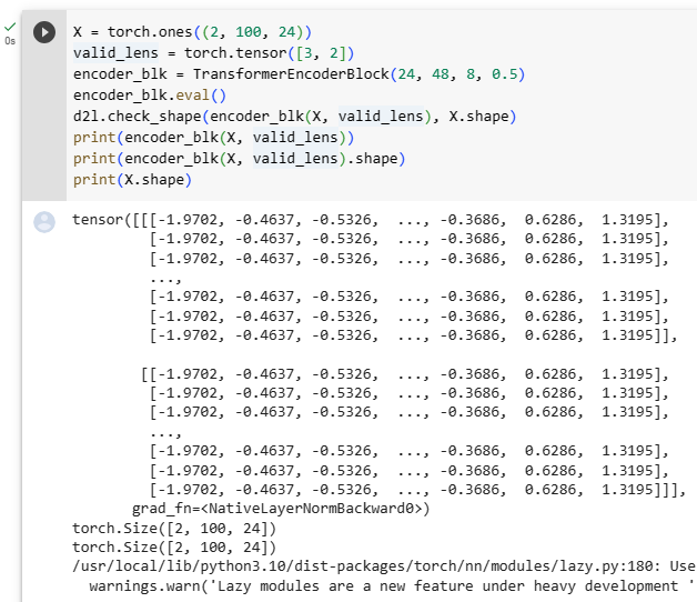
X = torch.ones((2, 100, 24))
valid_lens = torch.tensor([3, 2])
encoder_blk = TransformerEncoderBlock(24, 48, 8, 0.5)
encoder_blk.eval()
d2l.check_shape(encoder_blk(X, valid_lens), X.shape)
위 코드는 TransformerEncoderBlock 클래스의 동작을 테스트하는 부분입니다.
- X = torch.ones((2, 100, 24)): 크기가 (2, 100, 24)인 입력 데이터 X를 생성합니다. 이는 미니배치 크기가 2, 시퀀스 길이가 100, 피처 차원이 24인 데이터입니다.
- valid_lens = torch.tensor([3, 2]): 유효한 시퀀스 길이를 나타내는 텐서를 생성합니다. 이 예에서 첫 번째 시퀀스의 길이는 3, 두 번째 시퀀스의 길이는 2입니다.
- encoder_blk = TransformerEncoderBlock(24, 48, 8, 0.5): TransformerEncoderBlock 클래스를 생성합니다. 인코더 블록의 입력 차원은 24, 피드포워드 신경망의 은닉 상태 크기는 48, 어텐션 헤드 수는 8, 드롭아웃 비율은 0.5로 설정됩니다.
- encoder_blk.eval(): 모델을 평가 모드로 설정합니다. 이는 드롭아웃 레이어 등의 동작을 평가 모드로 변경하여 예측 결과의 안정성을 높이는 역할을 합니다.
- d2l.check_shape(encoder_blk(X, valid_lens), X.shape): encoder_blk에 입력 데이터 X와 유효한 시퀀스 길이 valid_lens를 입력하여 인코더 블록을 테스트합니다. 그 결과로 얻은 출력의 형상을 기존 입력 데이터 X의 형상과 비교하여 일치하는지를 확인합니다. 이를 통해 인코더 블록이 올바르게 동작하는지 검증합니다.
In the following Transformer encoder implementation, we stack num_blks instances of the above TransformerEncoderBlock classes. Since we use the fixed positional encoding whose values are always between -1 and 1, we multiply values of the learnable input embeddings by the square root of the embedding dimension to rescale before summing up the input embedding and the positional encoding.
다음 Transformer Encoder 구현에서는 위의 TransformerEncoderBlock 클래스의 num_blks 인스턴스를 쌓습니다. 값이 항상 -1과 1 사이인 fixed positional encoding을 사용하기 때문에 input embedding과 positional encoding을 합산하기 전에 학습 가능한 input embedding의 값에 embedding dimension의 제곱근을 곱하여 크기를 조정합니다.
class TransformerEncoder(d2l.Encoder):  #@save
    """The Transformer encoder."""
    def __init__(self, vocab_size, num_hiddens, ffn_num_hiddens,
                 num_heads, num_blks, dropout, use_bias=False):
        super().__init__()
        self.num_hiddens = num_hiddens
        self.embedding = nn.Embedding(vocab_size, num_hiddens)
        self.pos_encoding = d2l.PositionalEncoding(num_hiddens, dropout)
        self.blks = nn.Sequential()
        for i in range(num_blks):
            self.blks.add_module("block"+str(i), TransformerEncoderBlock(
                num_hiddens, ffn_num_hiddens, num_heads, dropout, use_bias))

    def forward(self, X, valid_lens):
        # Since positional encoding values are between -1 and 1, the embedding
        # values are multiplied by the square root of the embedding dimension
        # to rescale before they are summed up
        X = self.pos_encoding(self.embedding(X) * math.sqrt(self.num_hiddens))
        self.attention_weights = [None] * len(self.blks)
        for i, blk in enumerate(self.blks):
            X = blk(X, valid_lens)
            self.attention_weights[
                i] = blk.attention.attention.attention_weights
        return X
위 코드는 TransformerEncoder 클래스의 정의입니다. 이 클래스는 Transformer의 인코더 부분을 구성합니다.
- vocab_size, num_hiddens, ffn_num_hiddens, num_heads, num_blks, dropout, use_bias=False: 다양한 매개변수들이 클래스의 생성자에 전달됩니다. 이들은 인코더의 구성 및 하이퍼파라미터 설정에 사용됩니다.
- self.embedding = nn.Embedding(vocab_size, num_hiddens): 입력 토큰을 임베딩하기 위한 임베딩 레이어를 생성합니다. 임베딩 차원은 num_hiddens로 설정됩니다.
- self.pos_encoding = d2l.PositionalEncoding(num_hiddens, dropout): 위치 인코딩을 수행하기 위한 위치 인코딩 레이어를 생성합니다. 위치 인코딩은 임베딩 된 토큰 벡터에 추가되어 위치 정보를 제공합니다.
- self.blks = nn.Sequential(): 여러 개의 TransformerEncoderBlock 블록을 연결하여 시퀀스를 처리하는데 사용됩니다. nn.Sequential을 사용하여 블록을 연결합니다.
- for i in range(num_blks): ...: 입력으로 받은 num_blks 수만큼 루프를 돌며 TransformerEncoderBlock 블록을 추가합니다. 블록의 인수들은 클래스 생성자로부터 전달받은 하이퍼파라미터들로 설정됩니다.
- def forward(self, X, valid_lens): ...: 인코더의 순전파를 정의합니다. 입력 X와 유효한 시퀀스 길이 valid_lens를 받아서 처리한 후 결과를 반환합니다. 순전파 과정에서 임베딩, 위치 인코딩, 그리고 여러 개의 TransformerEncoderBlock 블록을 순차적으로 통과하게 됩니다.
- X = self.pos_encoding(self.embedding(X) * math.sqrt(self.num_hiddens)): 입력 X를 임베딩하고 위치 인코딩을 적용합니다. 임베딩 된 토큰 벡터에 위치 인코딩을 더하고, 임베딩 차원의 제곱근을 곱해줍니다.
- self.attention_weights = [None] * len(self.blks): 각 블록의 어텐션 가중치를 저장하는 빈 리스트를 생성합니다.
- for i, blk in enumerate(self.blks): ...: 연결된 블록들을 순회하며 각 블록에 X와 유효한 시퀀스 길이 valid_lens를 입력으로 전달하여 순전파를 수행합니다. 또한, 각 블록의 어텐션 가중치를 self.attention_weights에 저장합니다.
- return X: 최종적으로 모든 블록을 통과한 결과를 반환합니다.
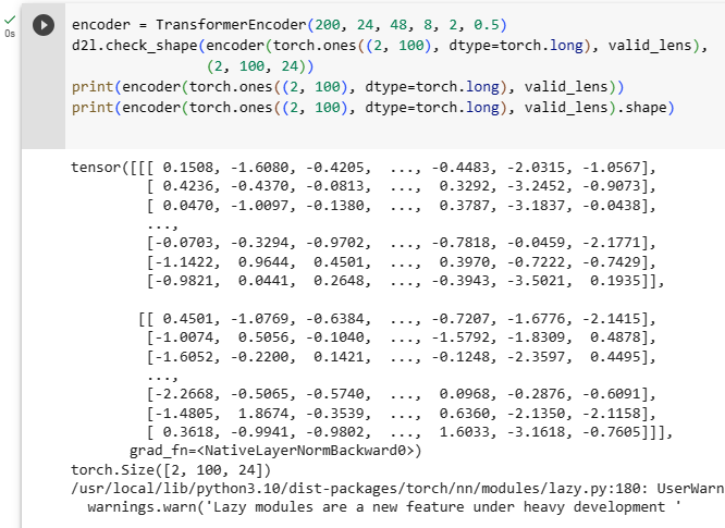
Below we specify hyperparameters to create a two-layer Transformer encoder. The shape of the Transformer encoder output is (batch size, number of time steps, num_hiddens).
아래에서 하이퍼파라미터를 지정하여 2계층 트랜스포머 인코더를 생성합니다. Transformer 인코더 출력의 shape 은 (배치 크기, 시간 단계 수, num_hiddens)입니다.
encoder = TransformerEncoder(200, 24, 48, 8, 2, 0.5)
d2l.check_shape(encoder(torch.ones((2, 100), dtype=torch.long), valid_lens),
                (2, 100, 24))
위 코드는 TransformerEncoder 클래스의 인스턴스를 생성하고, 해당 인스턴스를 사용하여 입력 데이터의 인코딩을 계산하고 결과의 형상을 확인하는 과정을 나타냅니다.
- encoder = TransformerEncoder(200, 24, 48, 8, 2, 0.5): TransformerEncoder 클래스의 인스턴스를 생성합니다. 생성자에 다양한 하이퍼파라미터를 전달하여 인코더의 구성을 설정합니다. 여기서는 입력 어휘 크기(vocab_size)를 200, 은닉 차원(num_hiddens)을 24, 피드포워드 신경망 내부 은닉 차원(ffn_num_hiddens)을 48, 어텐션 헤드 수(num_heads)를 8, 블록 수(num_blks)를 2, 드롭아웃 비율(dropout)을 0.5로 설정합니다.
- d2l.check_shape(encoder(torch.ones((2, 100), dtype=torch.long), valid_lens),(2, 100, 24)): 생성한 인코더 객체를 사용하여 입력 데이터의 인코딩을 계산하고 결과의 형상을 확인합니다. 여기서는 입력 데이터의 형상을 (2, 100)로 가정하고, 유효한 시퀀스 길이 정보인 valid_lens를 함께 전달합니다. 그 결과로 얻은 인코딩의 형상을 (2, 100, 24)로 확인합니다.
11.7.5. Decoder
As shown in Fig. 11.7.1, the Transformer decoder is composed of multiple identical layers. Each layer is implemented in the following TransformerDecoderBlock class, which contains three sublayers: decoder self-attention, encoder-decoder attention, and positionwise feed-forward networks. These sublayers employ a residual connection around them followed by layer normalization.
그림 11.7.1과 같이 Transformer 디코더는 여러 개의 동일한(identical ) 레이어로 구성됩니다. 각 계층은 다음 TransformerDecoderBlock 클래스에서 구현되며 여기에는, decoder self-attention, encoder-decoder attention 및 positionwise feed-forward networks 등 세 가지 sublayers이 포함됩니다. 이러한 sublayers 은 layer normalization가 뒤따르는 잔여 연결(residual connection)을 사용합니다.
As we described earlier in this section, in the masked multi-head decoder self-attention (the first sublayer), queries, keys, and values all come from the outputs of the previous decoder layer. When training sequence-to-sequence models, tokens at all the positions (time steps) of the output sequence are known. However, during prediction the output sequence is generated token by token; thus, at any decoder time step only the generated tokens can be used in the decoder self-attention. To preserve auto-regression in the decoder, its masked self-attention specifies dec_valid_lens so that any query only attends to all positions in the decoder up to the query position.
이 섹션의 앞부분에서 설명한 것처럼 masked multi-head decoder 에서 self-attention(첫 번째 하위 계층), 쿼리, 키 및 값은 모두 이전 디코더 계층의 출력에서 옵니다. sequence-to-sequence 모델을 교육할 때 출력 시퀀스의 모든 위치(시간 단계)에 있는 토큰이 알려져 있습니다. 그러나 예측 중에는 출력 시퀀스가 토큰별로 생성됩니다. 따라서 모든 디코더 시간 단계에서 생성된 토큰만 decoder self-attention에서 사용할 수 있습니다. 디코더에서 자동 회귀 auto-regression를 유지하기 위해 masked self-attention는 모든 쿼리가 디코더의 해당 쿼리까지의 모든 positions 에만 attends 하도록 dec_valid_lens를 지정합니다.
class TransformerDecoderBlock(nn.Module):
    # The i-th block in the Transformer decoder
    def __init__(self, num_hiddens, ffn_num_hiddens, num_heads, dropout, i):
        super().__init__()
        self.i = i
        self.attention1 = d2l.MultiHeadAttention(num_hiddens, num_heads,
                                                 dropout)
        self.addnorm1 = AddNorm(num_hiddens, dropout)
        self.attention2 = d2l.MultiHeadAttention(num_hiddens, num_heads,
                                                 dropout)
        self.addnorm2 = AddNorm(num_hiddens, dropout)
        self.ffn = PositionWiseFFN(ffn_num_hiddens, num_hiddens)
        self.addnorm3 = AddNorm(num_hiddens, dropout)

    def forward(self, X, state):
        enc_outputs, enc_valid_lens = state[0], state[1]
        # During training, all the tokens of any output sequence are processed
        # at the same time, so state[2][self.i] is None as initialized. When
        # decoding any output sequence token by token during prediction,
        # state[2][self.i] contains representations of the decoded output at
        # the i-th block up to the current time step
        if state[2][self.i] is None:
            key_values = X
        else:
            key_values = torch.cat((state[2][self.i], X), dim=1)
        state[2][self.i] = key_values
        if self.training:
            batch_size, num_steps, _ = X.shape
            # Shape of dec_valid_lens: (batch_size, num_steps), where every
            # row is [1, 2, ..., num_steps]
            dec_valid_lens = torch.arange(
                1, num_steps + 1, device=X.device).repeat(batch_size, 1)
        else:
            dec_valid_lens = None
        # Self-attention
        X2 = self.attention1(X, key_values, key_values, dec_valid_lens)
        Y = self.addnorm1(X, X2)
        # Encoder-decoder attention. Shape of enc_outputs:
        # (batch_size, num_steps, num_hiddens)
        Y2 = self.attention2(Y, enc_outputs, enc_outputs, enc_valid_lens)
        Z = self.addnorm2(Y, Y2)
        return self.addnorm3(Z, self.ffn(Z)), state
위 코드는 TransformerDecoderBlock 클래스를 정의하는 부분으로, Transformer 디코더 블록의 동작을 정의하고 있습니다. 이 블록은 Transformer 디코더 내에서 하나의 레이어를 나타내며, 여러 디코더 블록들이 연결되어 전체 디코더를 형성합니다.
- def __init__(self, num_hiddens, ffn_num_hiddens, num_heads, dropout, i): 디코더 블록의 생성자입니다. 다양한 하이퍼파라미터들과 블록의 순서를 나타내는 i 값을 받습니다.
- self.attention1 = d2l.MultiHeadAttention(num_hiddens, num_heads, dropout): 첫 번째 세트의 멀티헤드 어텐션을 생성합니다. 자기 어텐션입니다.
- self.addnorm1 = AddNorm(num_hiddens, dropout): 첫 번째 레이어 정규화와 잔차 연결을 위한 클래스 AddNorm을 생성합니다.
- self.attention2 = d2l.MultiHeadAttention(num_hiddens, num_heads, dropout): 두 번째 세트의 멀티헤드 어텐션을 생성합니다. 인코더-디코더 어텐션입니다.
- self.addnorm2 = AddNorm(num_hiddens, dropout): 두 번째 레이어 정규화와 잔차 연결을 위한 클래스 AddNorm을 생성합니다.
- self.ffn = PositionWiseFFN(ffn_num_hiddens, num_hiddens): 포지션 와이즈 피드포워드 네트워크를 생성합니다.
- self.addnorm3 = AddNorm(num_hiddens, dropout): 세 번째 레이어 정규화와 잔차 연결을 위한 클래스 AddNorm을 생성합니다.
- def forward(self, X, state): 디코더 블록의 순전파 함수입니다. 입력 데이터 X와 이전 상태 state를 받습니다.
- enc_outputs, enc_valid_lens = state[0], state[1]: 상태에서 인코더 출력과 유효한 시퀀스 길이를 가져옵니다.
- if state[2][self.i] is None:: 디코딩 중인 경우와 훈련 중인 경우에 따라서 어텐션 키 밸류 값을 설정합니다.
- if self.training:: 훈련 중인 경우입니다.
- batch_size, num_steps, _ = X.shape: 입력 데이터의 배치 크기와 시퀀스 길이를 가져옵니다.
- dec_valid_lens = torch.arange(1, num_steps + 1, device=X.device).repeat(batch_size, 1): 훈련 중인 경우, 유효한 시퀀스 길이 정보를 생성합니다.
- X2 = self.attention1(X, key_values, key_values, dec_valid_lens): 자기 어텐션 연산을 수행합니다.
- Y = self.addnorm1(X, X2): 첫 번째 어텐션 결과와 입력 데이터를 더하고 레이어 정규화를 수행합니다.
- Y2 = self.attention2(Y, enc_outputs, enc_outputs, enc_valid_lens): 인코더-디코더 어텐션 연산을 수행합니다.
- Z = self.addnorm2(Y, Y2): 두 번째 어텐션 결과와 이전 결과를 더하고 레이어 정규화를 수행합니다.
- return self.addnorm3(Z, self.ffn(Z)), state: 세 번째 어텐션 결과와 포지션 와이즈 피드포워드 네트워크를 수행한 결과를 더하고 레이어 정규화를 수행한 최종 결과와 상태를 반환합니다.
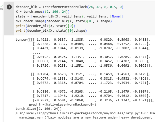
To facilitate scaled dot-product operations in the encoder-decoder attention and addition operations in the residual connections, the feature dimension (num_hiddens) of the decoder is the same as that of the encoder.
인코더-디코더 어텐션에서 scaled dot-product operations 와 residual connections에서 addition operations을 용이하게 하기 위해 디코더의 feature dimension(num_hiddens)은 인코더의 feature dimension과 동일합니다.
decoder_blk = TransformerDecoderBlock(24, 48, 8, 0.5, 0)
X = torch.ones((2, 100, 24))
state = [encoder_blk(X, valid_lens), valid_lens, [None]]
d2l.check_shape(decoder_blk(X, state)[0], X.shape)
위 코드는 TransformerDecoderBlock 클래스의 인스턴스를 생성하고, 디코더 블록의 순전파를 통해 출력의 형상을 확인하는 과정을 보여주고 있습니다.
- decoder_blk = TransformerDecoderBlock(24, 48, 8, 0.5, 0): 디코더 블록 클래스 TransformerDecoderBlock의 인스턴스를 생성합니다. 이 때 필요한 하이퍼파라미터들을 설정합니다.
- X = torch.ones((2, 100, 24)): 입력 데이터 X를 생성합니다. 이 예시에서는 2개의 배치, 100개의 시퀀스 길이, 그리고 24차원의 임베딩을 가지는 입력 데이터를 생성합니다.
- state = [encoder_blk(X, valid_lens), valid_lens, [None]]: 인코더 블록의 순전파를 통해 인코더의 출력과 유효한 시퀀스 길이를 가지는 상태를 생성합니다. 마지막 리스트는 초기에 디코더 블록 내에서 사용하는 어텐션 키 밸류 값입니다.
- d2l.check_shape(decoder_blk(X, state)[0], X.shape): 디코더 블록의 순전파를 통해 출력의 형상을 확인합니다. 디코더 블록의 입력으로 X와 이전 상태 state를 주고, 출력의 형상을 입력 데이터 X의 형상과 비교합니다.
Now we construct the entire Transformer decoder composed of num_blks instances of TransformerDecoderBlock. In the end, a fully connected layer computes the prediction for all the vocab_size possible output tokens. Both of the decoder self-attention weights and the encoder-decoder attention weights are stored for later visualization.
이제 TransformerDecoderBlock의 num_blks 인스턴스로 구성된 전체 Transformer 디코더를 구성합니다. 마지막에 fully connected layer 모든 vocab_size 가능한 출력 토큰에 대한 예측을 계산합니다. self-attention weights와 encoder-decoder attention weights 모두 나중에 시각화하기 위해 저장됩니다.
class TransformerDecoder(d2l.AttentionDecoder):
    def __init__(self, vocab_size, num_hiddens, ffn_num_hiddens, num_heads,
                 num_blks, dropout):
        super().__init__()
        self.num_hiddens = num_hiddens
        self.num_blks = num_blks
        self.embedding = nn.Embedding(vocab_size, num_hiddens)
        self.pos_encoding = d2l.PositionalEncoding(num_hiddens, dropout)
        self.blks = nn.Sequential()
        for i in range(num_blks):
            self.blks.add_module("block"+str(i), TransformerDecoderBlock(
                num_hiddens, ffn_num_hiddens, num_heads, dropout, i))
        self.dense = nn.LazyLinear(vocab_size)

    def init_state(self, enc_outputs, enc_valid_lens):
        return [enc_outputs, enc_valid_lens, [None] * self.num_blks]

    def forward(self, X, state):
        X = self.pos_encoding(self.embedding(X) * math.sqrt(self.num_hiddens))
        self._attention_weights = [[None] * len(self.blks) for _ in range (2)]
        for i, blk in enumerate(self.blks):
            X, state = blk(X, state)
            # Decoder self-attention weights
            self._attention_weights[0][
                i] = blk.attention1.attention.attention_weights
            # Encoder-decoder attention weights
            self._attention_weights[1][
                i] = blk.attention2.attention.attention_weights
        return self.dense(X), state

    @property
    def attention_weights(self):
        return self._attention_weights
위 코드는 TransformerDecoder 클래스를 정의하고, 해당 디코더의 동작을 구현한 것입니다.
- class TransformerDecoder(d2l.AttentionDecoder): TransformerDecoder 클래스를 정의하며, d2l.AttentionDecoder 클래스를 상속받습니다. 이 클래스는 어텐션 메커니즘을 사용하는 디코더를 나타냅니다.
- def __init__(self, vocab_size, num_hiddens, ffn_num_hiddens, num_heads, num_blks, dropout): 초기화 함수에서 필요한 하이퍼파라미터와 레이어를 설정합니다.
- def init_state(self, enc_outputs, enc_valid_lens): 디코더의 상태를 초기화하는 함수입니다. 인코더의 출력과 유효한 시퀀스 길이를 받아 초기 상태를 생성합니다.
- def forward(self, X, state): 순전파 함수를 정의합니다. 입력 X와 현재 상태 state를 받아 디코더 블록들을 통과시키고, 디코더의 출력과 다음 상태를 반환합니다. 각 블록에서의 어텐션 가중치를 _attention_weights에 저장합니다.
- @property 데코레이터를 통해 attention_weights 함수를 프로퍼티로 정의합니다. 이 함수는 _attention_weights를 반환하며, 각 블록에서의 어텐션 가중치를 포함합니다.
11.7.6. Training
Let’s instantiate an encoder-decoder model by following the Transformer architecture. Here we specify that both the Transformer encoder and the Transformer decoder have 2 layers using 4-head attention. Similar to Section 10.7.6, we train the Transformer model for sequence to sequence learning on the English-French machine translation dataset.
Transformer 아키텍처를 따라 인코더-디코더 모델을 인스턴스화해 보겠습니다. 여기서 우리는 Transformer 인코더와 Transformer 디코더 모두 4-head Attention을 사용하는 2개의 레이어를 가지도록 설정합니다. 섹션 10.7.6과 유사하게 영어-프랑스어 기계 번역 데이터 세트에서 sequence to sequence 학습을 위해 Transformer 모델을 훈련합니다.
data = d2l.MTFraEng(batch_size=128)
num_hiddens, num_blks, dropout = 256, 2, 0.2
ffn_num_hiddens, num_heads = 64, 4
encoder = TransformerEncoder(
    len(data.src_vocab), num_hiddens, ffn_num_hiddens, num_heads,
    num_blks, dropout)
decoder = TransformerDecoder(
    len(data.tgt_vocab), num_hiddens, ffn_num_hiddens, num_heads,
    num_blks, dropout)
model = d2l.Seq2Seq(encoder, decoder, tgt_pad=data.tgt_vocab['<pad>'],
                    lr=0.0015)
trainer = d2l.Trainer(max_epochs=30, gradient_clip_val=1, num_gpus=1)
trainer.fit(model, data)
위 코드는 d2l 라이브러리를 사용하여 Transformer 모델을 기반으로한 기계 번역 모델을 학습하는 과정을 나타냅니다.
- data = d2l.MTFraEng(batch_size=128): 기계 번역을 위한 데이터셋을 생성하고 배치 크기를 128로 설정합니다.
- num_hiddens, num_blks, dropout = 256, 2, 0.2: 모델의 하이퍼파라미터를 설정합니다. num_hiddens는 임베딩 및 어텐션의 히든 노드 개수, num_blks는 인코더와 디코더의 블록 개수, dropout은 드롭아웃 확률을 의미합니다.
- ffn_num_hiddens, num_heads = 64, 4: Feed-Forward Network (FFN)과 어텐션의 헤드 개수를 설정합니다.
- encoder = TransformerEncoder(...): 인코더를 생성합니다. 입력 어휘 크기, 히든 노드 개수, FFN의 히든 노드 개수, 어텐션 헤드 개수, 블록 개수, 드롭아웃 확률을 인자로 전달합니다.
- decoder = TransformerDecoder(...): 디코더를 생성합니다. 출력 어휘 크기, 히든 노드 개수, FFN의 히든 노드 개수, 어텐션 헤드 개수, 블록 개수, 드롭아웃 확률을 인자로 전달합니다.
- model = d2l.Seq2Seq(...): Seq2Seq 모델을 생성합니다. 인코더, 디코더, 타겟 패딩 토큰 ID, 학습률 등을 설정합니다.
- trainer = d2l.Trainer(...): 모델 학습을 위한 트레이너를 생성합니다. 최대 에포크 수, 그래디언트 클리핑 값, GPU 개수 등을 설정합니다.
- trainer.fit(model, data): 트레이너를 사용하여 모델을 데이터에 학습시킵니다.


After training, we use the Transformer model to translate a few English sentences into French and compute their BLEU scores.
학습 후 Transformer 모델을 사용하여 몇 개의 영어 문장을 프랑스어로 번역하고 BLEU 점수를 계산합니다.
engs = ['go .', 'i lost .', 'he\'s calm .', 'i\'m home .']
fras = ['va !', 'j\'ai perdu .', 'il est calme .', 'je suis chez moi .']
preds, _ = model.predict_step(
    data.build(engs, fras), d2l.try_gpu(), data.num_steps)
for en, fr, p in zip(engs, fras, preds):
    translation = []
    for token in data.tgt_vocab.to_tokens(p):
        if token == '<eos>':
            break
        translation.append(token)
    print(f'{en} => {translation}, bleu,'
          f'{d2l.bleu(" ".join(translation), fr, k=2):.3f}')
위 코드는 학습된 기계 번역 Transformer 모델을 사용하여 주어진 영어 문장을 프랑스어로 번역하고 BLEU 점수를 계산하는 과정을 나타냅니다.
- engs와 fras: 번역할 영어 문장과 정답 프랑스어 문장들의 리스트입니다.
- preds, _ = model.predict_step(...): 학습된 모델을 사용하여 주어진 영어 문장을 프랑스어로 번역합니다. data.build 함수를 사용하여 입력 데이터를 생성하고, d2l.try_gpu()를 통해 GPU를 사용하도록 설정합니다. data.num_steps는 문장의 최대 길이입니다. 번역 결과와 기타 정보가 preds와 _ 변수에 저장됩니다.
- for en, fr, p in zip(engs, fras, preds):: 번역된 결과를 영어 문장, 정답 프랑스어 문장, 번역된 프랑스어 문장과 함께 루프로 반복합니다.
- translation = []: 번역된 프랑스어 문장을 저장할 빈 리스트를 생성합니다.
- for token in data.tgt_vocab.to_tokens(p):: 번역된 프랑스어 문장의 토큰을 하나씩 확인합니다.
- if token == '<eos>':: 토큰이 <eos> (문장 종료 토큰)인 경우 반복을 종료합니다.
- translation.append(token): 토큰을 translation 리스트에 추가합니다.
- print(f'{en} => {translation}, bleu, ...: 영어 문장, 번역된 프랑스어 문장, BLEU 점수를 출력합니다. BLEU 점수는 d2l.bleu 함수를 사용하여 계산하며, 정답 프랑스어 문장과 번역된 프랑스어 문장을 비교합니다.
After training, we use the Transformer model to [translate a few English sentences] into French and compute their BLEU scores.
훈련 후에는 Transformer 모델을 사용하여 영어 문장 몇 개를 프랑스어로 번역하고 BLEU 점수를 계산합니다.
go . => ['va', '!'], bleu,1.000
i lost . => ["j'ai", 'perdu', '.'], bleu,1.000
he's calm . => ['calme', '.'], bleu,0.368
i'm home . => ['je', 'suis', 'chez', 'moi', '.'], bleu,1.000
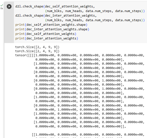
Let’s visualize the Transformer attention weights when translating the last English sentence into French. The shape of the encoder self-attention weights is (number of encoder layers, number of attention heads, num_steps or number of queries, num_steps or number of key-value pairs).
마지막 영어 문장을 프랑스어로 번역할 때 Transformer attention weights를 시각화해 보겠습니다. 인코더 self-attention weights의 형태는 (인코더 레이어 수, 어텐션 헤드 수, num_steps 또는 쿼리 수, num_steps 또는 키-값 쌍 수)입니다.
_, dec_attention_weights = model.predict_step(
    data.build([engs[-1]], [fras[-1]]), d2l.try_gpu(), data.num_steps, True)
enc_attention_weights = torch.cat(model.encoder.attention_weights, 0)
shape = (num_blks, num_heads, -1, data.num_steps)
enc_attention_weights = enc_attention_weights.reshape(shape)
d2l.check_shape(enc_attention_weights,
                (num_blks, num_heads, data.num_steps, data.num_steps))
위 코드는 모델의 self-attention 및 encoder-decoder attention 가중치를 확인하고 검사하는 과정을 나타냅니다.
- _, dec_attention_weights = model.predict_step(...): 주어진 영어 문장을 프랑스어로 번역하면서 두 가지의 attention 가중치를 반환합니다. data.build 함수로 입력 데이터를 생성하고, d2l.try_gpu()를 통해 GPU를 사용하도록 설정합니다. data.num_steps는 문장의 최대 길이입니다. True 파라미터는 attention 가중치를 반환하도록 지시합니다.
- enc_attention_weights = torch.cat(model.encoder.attention_weights, 0): 인코더의 self-attention 가중치를 모두 하나의 텐서로 결합합니다.
- shape = (num_blks, num_heads, -1, data.num_steps): 가중치의 모양을 지정합니다. num_blks는 블록의 수, num_heads는 head의 수, data.num_steps는 문장 길이입니다. -1은 다른 차원을 맞추고 남는 차원을 지정합니다.
- enc_attention_weights = enc_attention_weights.reshape(shape): 가중치 텐서의 모양을 지정한 shape로 재구성합니다.
- d2l.check_shape(enc_attention_weights, ...: 재구성된 가중치 텐서의 모양을 확인합니다. 정확한 모양은 num_blks, num_heads, 문장 길이, 문장 길이입니다. 이는 인코더 블록에서 self-attention 가중치의 모양을 검사하는 것입니다.


In the encoder self-attention, both queries and keys come from the same input sequence. Since padding tokens do not carry meaning, with specified valid length of the input sequence, no query attends to positions of padding tokens. In the following, two layers of multi-head attention weights are presented row by row. Each head independently attends based on a separate representation subspaces of queries, keys, and values.
인코더 self-attention에서 쿼리와 키는 모두 동일한 입력 시퀀스에서 나옵니다. 패딩 토큰은 의미를 전달하지 않으므로 입력 시퀀스의 지정된 유효 길이를 사용하면 패딩 토큰의 위치에 대한 query attends는 없습니다. 다음에서는 multi-head attention weights의 두 레이어가 행별로 표시됩니다. 각 헤드는 쿼리, 키 및 값의 별도 representation 하위 공간을 기반으로 독립적으로 attends 합니다.
d2l.show_heatmaps(
    enc_attention_weights.cpu(), xlabel='Key positions',
    ylabel='Query positions', titles=['Head %d' % i for i in range(1, 5)],
    figsize=(7, 3.5))
위 코드는 인코더의 self-attention 가중치를 시각화하는 과정을 나타냅니다.
- d2l.show_heatmaps(: d2l.show_heatmaps 함수를 호출하여 열쇠(Key) 위치와 질문(Query) 위치에 대한 인코더의 self-attention 가중치를 히트맵으로 표시합니다.
- enc_attention_weights.cpu(): 가중치 텐서를 CPU로 이동시킵니다. 이는 히트맵을 생성할 때 GPU와 호환되도록 하는 과정입니다.
- xlabel='Key positions', ylabel='Query positions': 히트맵의 x축과 y축에 레이블을 붙입니다. 여기서 x축은 Key 위치, y축은 Query 위치를 나타냅니다.
- titles=['Head %d' % i for i in range(1, 5)]: 각 히트맵의 제목을 지정합니다. 인코더 내의 각 head에 대한 히트맵을 생성할 것이며, 제목에는 head의 번호가 포함됩니다.
- figsize=(7, 3.5)): 생성되는 히트맵의 크기를 지정합니다. (7, 3.5)는 가로 7, 세로 3.5의 크기를 가진 히트맵을 생성하라는 의미입니다.
이렇게 하면 인코더 내의 self-attention 가중치가 여러 head 및 위치에 대해 시각화된 히트맵이 생성됩니다.


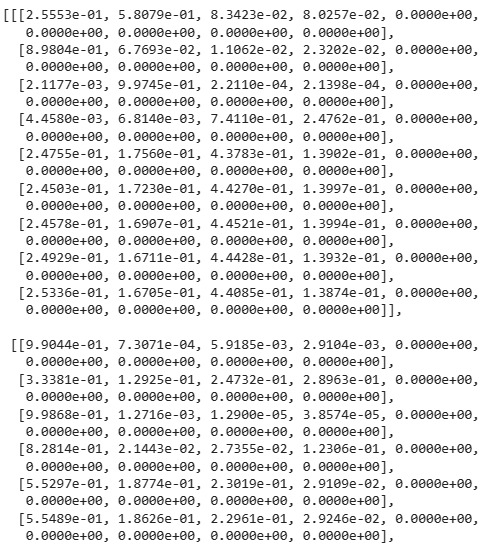
To visualize both the decoder self-attention weights and the encoder-decoder attention weights, we need more data manipulations. For example, we fill the masked attention weights with zero. Note that the decoder self-attention weights and the encoder-decoder attention weights both have the same queries: the beginning-of-sequence token followed by the output tokens and possibly end-of-sequence tokens.
decoder self-attention weights 와 encoder-decoder attention weights를 모두 시각화하려면 더 많은 데이터 조작이 필요합니다. 예를 들어 masked attention weights를 0으로 채웁니다. decoder self-attention weights와 encoder-decoder attention weights는 모두 동일한 쿼리를 가집니다. 즉, beginning-of-sequence token 다음에 output tokens 및 end-of-sequence tokens이 올 수 있습니다.
dec_attention_weights_2d = [head[0].tolist()
                            for step in dec_attention_weights
                            for attn in step for blk in attn for head in blk]
dec_attention_weights_filled = torch.tensor(
    pd.DataFrame(dec_attention_weights_2d).fillna(0.0).values)
shape = (-1, 2, num_blks, num_heads, data.num_steps)
dec_attention_weights = dec_attention_weights_filled.reshape(shape)
dec_self_attention_weights, dec_inter_attention_weights = \
    dec_attention_weights.permute(1, 2, 3, 0, 4)

d2l.check_shape(dec_self_attention_weights,
                (num_blks, num_heads, data.num_steps, data.num_steps))
d2l.check_shape(dec_inter_attention_weights,
                (num_blks, num_heads, data.num_steps, data.num_steps))
위 코드는 디코더의 self-attention 가중치와 인코더-디코더 attention 가중치를 시각화하기 위한 과정을 나타냅니다.
- dec_attention_weights_2d: 디코더의 self-attention 가중치를 2차원 리스트 형태로 변환합니다. 이는 향후 데이터 분석을 위한 과정입니다. 여기서 dec_attention_weights는 디코더의 attention 가중치입니다.
- dec_attention_weights_filled: 2차원 리스트를 이용해 누락된 값을 0.0으로 채운 텐서를 생성합니다. 이를 통해 향후 시각화를 진행할 때 빈 값을 처리할 수 있습니다.
- shape: 텐서의 형태를 재구성하기 위한 shape를 정의합니다. 5차원의 텐서 구조로 만들 것이며, 이는 디코더의 self-attention 및 인코더-디코더 attention 가중치에 대한 구조를 나타냅니다.
- dec_attention_weights: 위에서 만든 dec_attention_weights_filled 텐서를 shape에 맞게 재구성합니다. 이렇게 하면 디코더의 self-attention 및 인코더-디코더 attention 가중치가 적절한 구조로 저장됩니다.
- dec_self_attention_weights와 dec_inter_attention_weights: dec_attention_weights를 통해 생성된 텐서를 디코더의 self-attention 가중치와 인코더-디코더 attention 가중치로 분리합니다. 이를 위해 텐서의 차원을 조정하고 순서를 변경합니다.
- d2l.check_shape: 텐서의 형태를 확인하는 함수를 사용하여 디코더의 self-attention 가중치와 인코더-디코더 attention 가중치의 형태를 검증합니다. 각각의 형태는 (num_blks, num_heads, data.num_steps, data.num_steps)와 같아야 합니다.
이러한 과정을 통해 디코더의 self-attention 가중치와 인코더-디코더 attention 가중치가 적절한 형태로 처리되고 시각화될 준비가 완료됩니다.

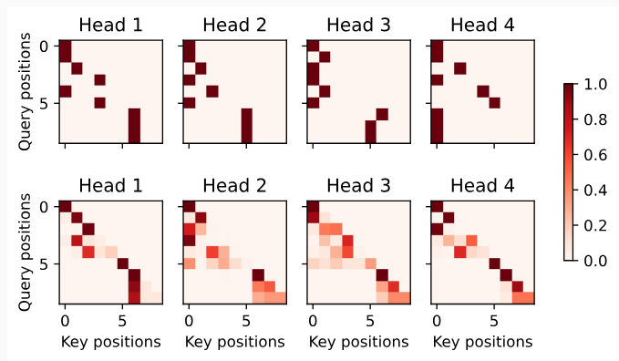
Due to the auto-regressive property of the decoder self-attention, no query attends to key-value pairs after the query position.
디코더 self-attention의 auto-regressive 속성으로 인해 query position 이후의 ey-value pairs에 query attends는 없습니다.
d2l.show_heatmaps(
    dec_self_attention_weights[:, :, :, :],
    xlabel='Key positions', ylabel='Query positions',
    titles=['Head %d' % i for i in range(1, 5)], figsize=(7, 3.5))
위 코드는 디코더의 self-attention 가중치를 열쇠 (Key) 위치와 질의 (Query) 위치에 대한 열과 행으로 시각화합니다.
- dec_self_attention_weights[:, :, :, :]: 디코더의 self-attention 가중치를 해당하는 범위 내에서 선택합니다. 이렇게 함으로써 시각화할 때 필요한 구간을 선택하게 됩니다.
- xlabel과 ylabel: 시각화 결과의 x축과 y축에 표시될 레이블을 설정합니다. 이 경우 "Key positions"와 "Query positions"로 설정되어 key 위치와 query 위치를 의미합니다.
- titles: 시각화된 각 히트맵의 제목을 설정합니다. 여기서는 "Head 1", "Head 2", "Head 3", "Head 4"와 같이 각 헤드에 대한 정보를 표시합니다.
- figsize: 시각화된 히트맵의 크기를 설정합니다. (7, 3.5)로 설정되어 있으며 가로 7, 세로 3.5의 크기로 히트맵이 표시됩니다.
이를 통해 디코더의 self-attention 가중치가 열쇠 위치와 질의 위치에 따라 시각화되며, 각각의 헤드에 대한 정보도 함께 나타납니다.

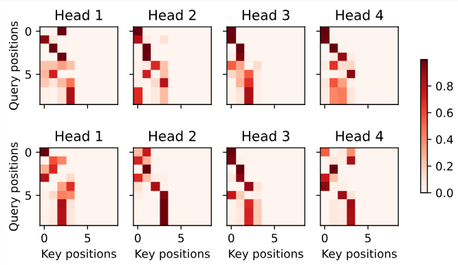
Similar to the case in the encoder self-attention, via the specified valid length of the input sequence, no query from the output sequence attends to those padding tokens from the input sequence.
인코더 self-attention의 경우와 유사하게 입력 시퀀스의 지정된 유효 길이를 통해 output sequence에서 input sequence에서 온 padding tokens로의 query는 없습니다.
d2l.show_heatmaps(
    dec_inter_attention_weights, xlabel='Key positions',
    ylabel='Query positions', titles=['Head %d' % i for i in range(1, 5)],
    figsize=(7, 3.5))
이 코드는 디코더의 self-attention 가중치를 시각화하는 과정을 보여줍니다. 이 코드를 하나씩 설명해보겠습니다.
- dec_self_attention_weights[:, :, :, :]: 디코더의 self-attention 가중치를 선택합니다. 이것은 시각화를 위해 해당 가중치의 특정 부분을 선택하는 것입니다.
- xlabel 및 ylabel: 시각화된 히트맵의 x축 및 y축에 나타날 레이블을 설정합니다. 이 경우 "Key positions"와 "Query positions"로 설정되어 열쇠 (Key) 위치 및 질의 (Query) 위치를 나타냅니다.
- titles: 시각화된 히트맵 각각의 제목을 설정합니다. 여기에서는 "Head 1", "Head 2", "Head 3", "Head 4"와 같이 각 헤드에 대한 정보를 보여줍니다.
- figsize: 시각화된 히트맵의 크기를 설정합니다. (7, 3.5)로 설정되어 있으며 가로 7, 세로 3.5의 크기로 히트맵이 표시됩니다.
이 코드의 목적은 디코더의 self-attention 가중치를 시각화하여 열쇠 위치와 질의 위치 간의 관계를 파악하고, 각 헤드에 대한 정보를 시각적으로 확인하는 것입니다.

Although the Transformer architecture was originally proposed for sequence-to-sequence learning, as we will discover later in the book, either the Transformer encoder or the Transformer decoder is often individually used for different deep learning tasks.
Transformer 아키텍처는 원래 sequence-to-sequence 학습을 위해 제안되었지만 이 책의 뒷부분에서 알게 되겠지만 Transformer 인코더 또는 Transformer 디코더는 서로 다른 딥 러닝 작업에 개별적으로 사용되는 경우가 많습니다.
11.7.7. Summary
The Transformer is an instance of the encoder-decoder architecture, though either the encoder or the decoder can be used individually in practice. In the Transformer architecture, multi-head self-attention is used for representing the input sequence and the output sequence, though the decoder has to preserve the auto-regressive property via a masked version. Both the residual connections and the layer normalization in the Transformer are important for training a very deep model. The positionwise feed-forward network in the Transformer model transforms the representation at all the sequence positions using the same MLP.
Transformer는 인코더-디코더 아키텍처의 인스턴스이지만 실제로는 인코더 또는 디코더를 개별적으로 사용할 수 있습니다. 트랜스포머 아키텍처에서 multi-head self-attention은 입력 시퀀스와 출력 시퀀스를 나타내는 데 사용되지만 디코더는 masked version을 통해 자동 회귀 속성을 보존해야 합니다. Transformer의 residual connections과 layer normalization는 모두 아주 deep 한 model을 교육하는 데 중요합니다. Transformer 모델의 positionwise feed-forward network는 동일한 MLP를 사용하여 모든 시퀀스 위치에서 representation 을 변환합니다.
11.7.8. Exercises
- Train a deeper Transformer in the experiments. How does it affect the training speed and the translation performance?
- Is it a good idea to replace scaled dot-product attention with additive attention in the Transformer? Why?
- For language modeling, should we use the Transformer encoder, decoder, or both? How to design this method?
- What can be challenges to Transformers if input sequences are very long? Why?
- How to improve computational and memory efficiency of Transformers? Hint: you may refer to the survey paper by Tay et al. (2020).
'Dive into Deep Learning > D2L Attention Mechanisms and Transformer' 카테고리의 다른 글
| D2L - 11.9. Large-Scale Pretraining with Transformers (0) | 2023.08.10 |
|---|---|
| D2L - 11.8. Transformers for Vision (0) | 2023.08.10 |
| D2L - 11.6. Self-Attention and Positional Encoding (0) | 2023.08.09 |
| D2L - 11.5. Multi-Head Attention (0) | 2023.08.08 |
| D2L - 11.4. The Bahdanau Attention Mechanism (1) | 2023.08.08 |
| D2L - 11.3. Attention Scoring Functions (0) | 2023.08.07 |
| D2L - 11.2. Attention Pooling by Similarity (0) | 2023.08.06 |
| D2L - 11.1. Queries, Keys, and Values (0) | 2023.08.05 |
| D2L - 11. Attention Mechanisms and Transformers (0) | 2023.08.03 |