아래 내용은 ChatGPT와 MicroK8s 홈페이지에서 도움을 받아 진행한 내용입니다.
ChatGPT + https://microk8s.io/docs/install-windows
https://microk8s.io/docs/install-windows
microk8s.io
Installing Microk8s on Windows 11 Home is not directly supported. However, you can install Microk8s using the Windows Subsystem for Linux (WSL). Here are the steps to do so on Windows 11 Home:
- Install WSL:
- To use Linux on Windows, you must first install WSL. Run PowerShell as an administrator and enter the following command:
wsl --install
- This command installs WSL and typically installs a default Linux distribution, such as Ubuntu.
- To use Linux on Windows, you must first install WSL. Run PowerShell as an administrator and enter the following command:
- Update and Set Up WSL:
- WSL2 offers better performance for running Docker and Kubernetes. To upgrade to WSL2, execute:
wsl --set-default-version 2
- After installing WSL, you can install your preferred Linux distribution from the Microsoft Store, such as Ubuntu.
- WSL2 offers better performance for running Docker and Kubernetes. To upgrade to WSL2, execute:
- Prepare to Install Microk8s:
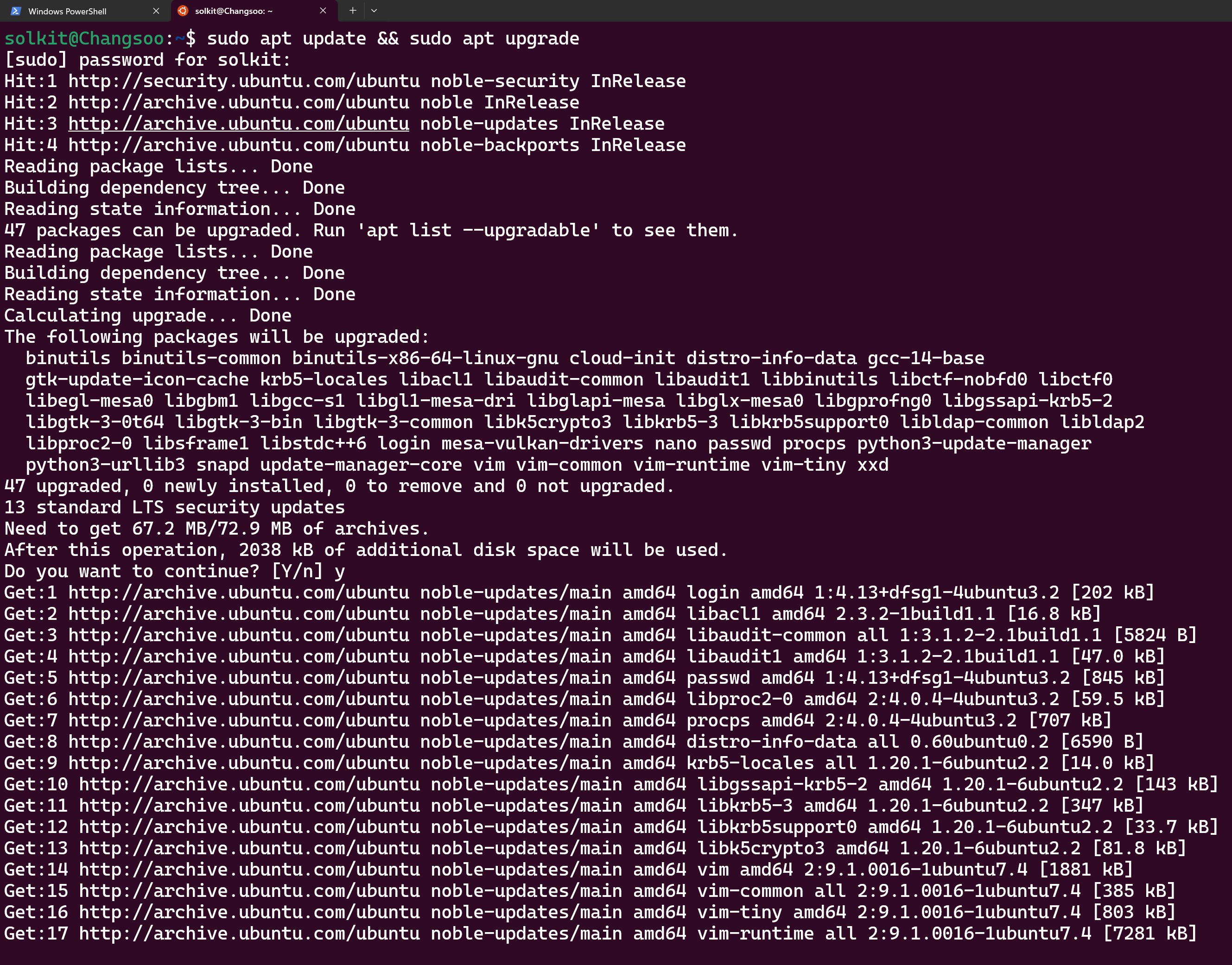
- Launch your Linux distribution and update your system:
sudo apt update && sudo apt upgrade
- Launch your Linux distribution and update your system:
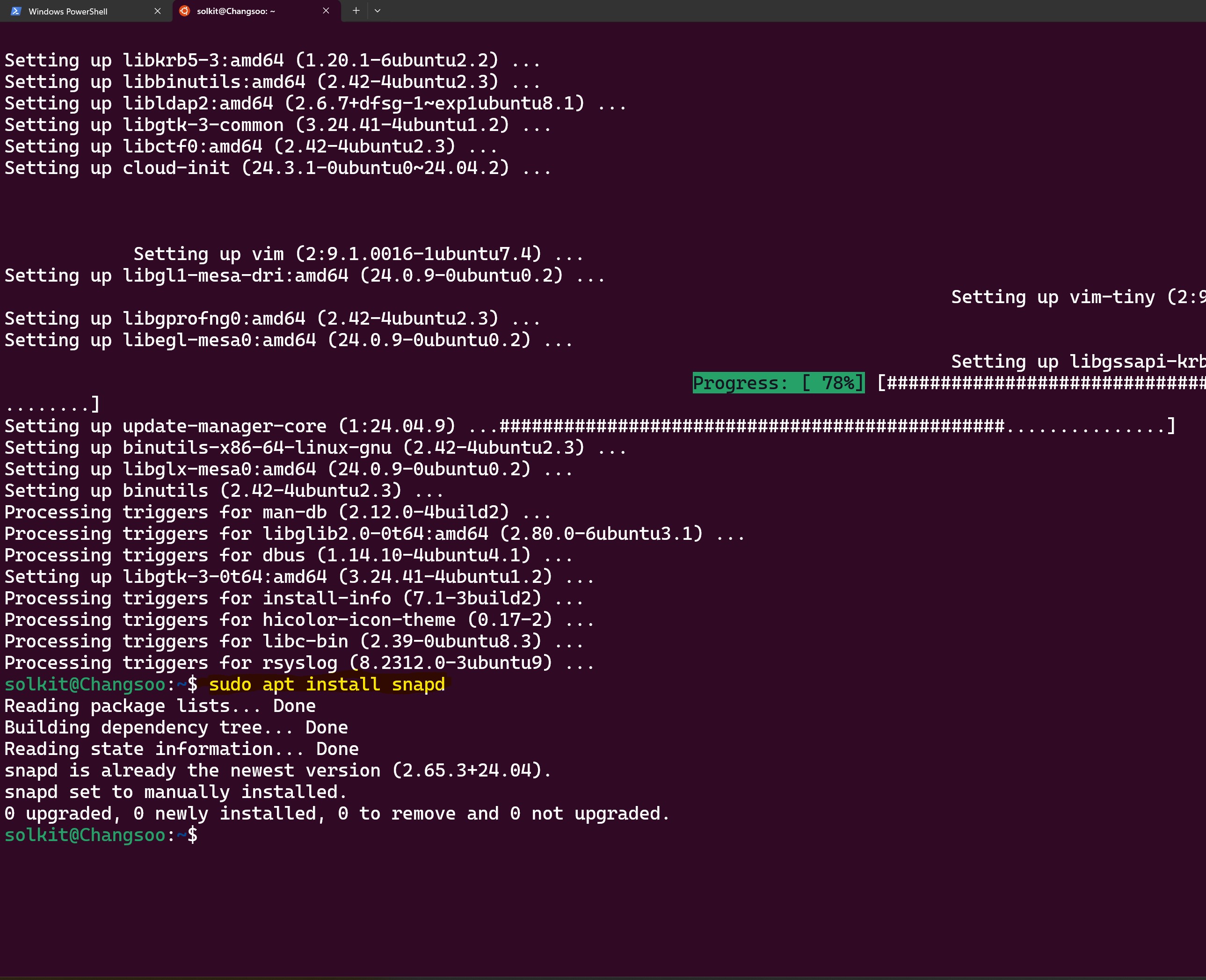
- Install Snap:
- If Snap is not pre-installed in Ubuntu, install it with:
sudo apt install snapd
- If Snap is not pre-installed in Ubuntu, install it with:
- Install Microk8s:
- Install Microk8s using the following command:
sudo snap install microk8s --classic
- After installation, add your user to the microk8s group to run Microk8s commands without sudo:
sudo usermod -a -G microk8s $USER sudo chown -f -R $USER ~/.kube
- Install Microk8s using the following command:
- Activate and Verify Microk8s:
- Start Microk8s and check its status:
microk8s start microk8s status --wait-ready
- Enable necessary Microk8s add-ons:
microk8s enable dns dashboard storage ingress
- Start Microk8s and check its status:
- Using Kubernetes with Microk8s:
- Microk8s wraps the familiar kubectl command, allowing you to perform typical Kubernetes operations. For example:
microk8s kubectl get all --all-namespaces
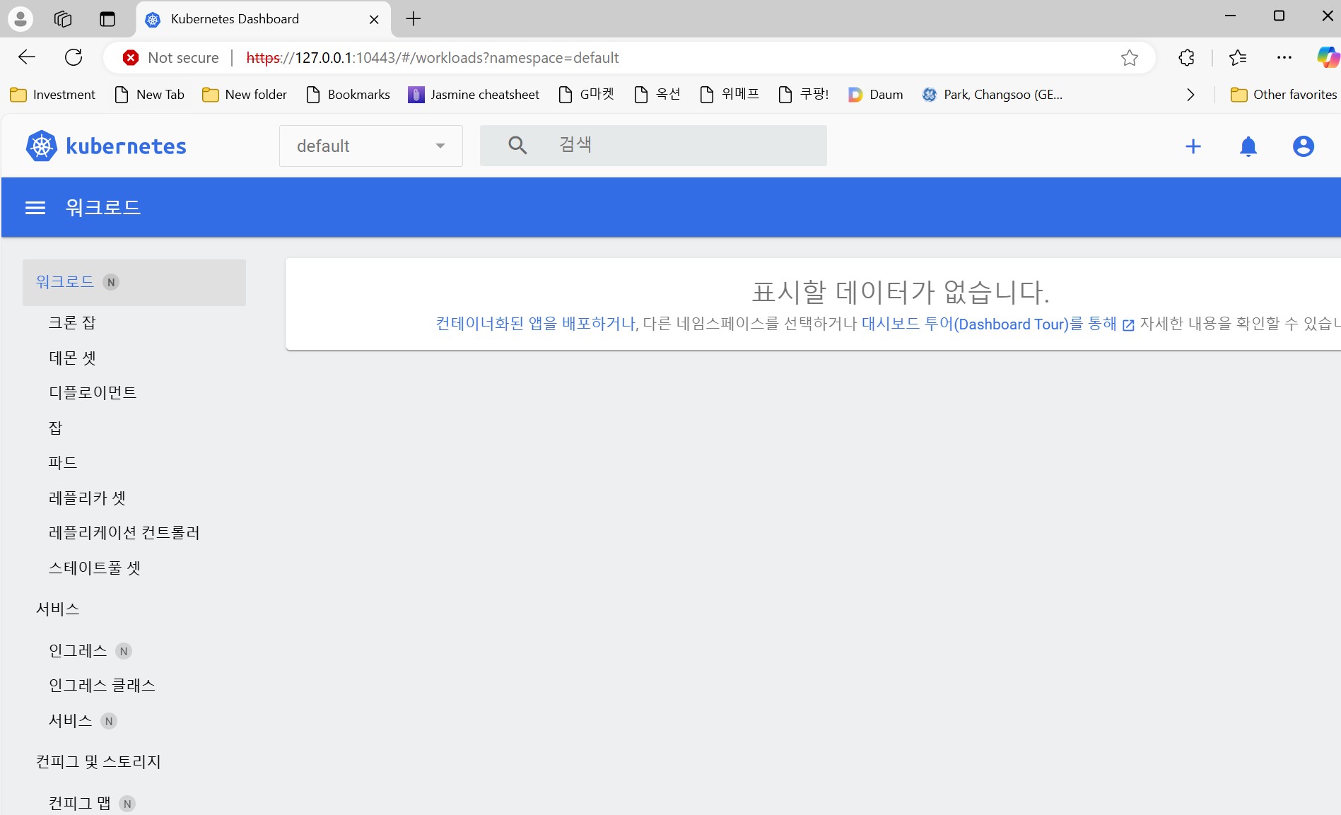
- Access the Kubernetes dashboard with:
microk8s dashboard-proxy
- Microk8s wraps the familiar kubectl command, allowing you to perform typical Kubernetes operations. For example:
- Start and Stop Kubernetes:
- When not using Microk8s, you can stop the Kubernetes services to conserve power and resources:
microk8s stop
- To restart the services:
microk8s start
- When not using Microk8s, you can stop the Kubernetes services to conserve power and resources:
These steps will help you successfully set up and start using Microk8s on Windows 11 Home through WSL.
===================================================================
Windows 11 Home에서 Microk8s를 직접 설치하는 것은 지원되지 않습니다. 그러나 Windows Subsystem for Linux (WSL)을 사용하여 Microk8s를 설치할 수 있습니다. 다음은 Windows 11 Home에서 Microk8s를 설치하는 단계입니다:
- WSL 설치하기:
- Windows에서 Linux 환경을 사용하기 위해 PowerShell을 관리자 권한으로 실행한 후 다음 명령어를 입력합니다:
wsl --install
- 이 명령어는 WSL을 설치하고 일반적으로 Ubuntu와 같은 기본 Linux 배포판을 자동으로 설치합니다.
- Windows에서 Linux 환경을 사용하기 위해 PowerShell을 관리자 권한으로 실행한 후 다음 명령어를 입력합니다:
- WSL 업데이트 및 설정:
- Docker와 Kubernetes를 실행하기 위한 더 나은 성능을 제공하는 WSL2로 업데이트하려면 다음 명령을 실행합니다:
wsl --set-default-version 2
- WSL 설치가 완료된 후, Microsoft Store에서 선호하는 Linux 배포판을 설치할 수 있습니다.
- Docker와 Kubernetes를 실행하기 위한 더 나은 성능을 제공하는 WSL2로 업데이트하려면 다음 명령을 실행합니다:
- Microk8s 설치 준비:
- Linux 배포판을 실행하고, 시스템을 최신 상태로 업데이트합니다:
sudo apt update && sudo apt upgrade
- Linux 배포판을 실행하고, 시스템을 최신 상태로 업데이트합니다:
- Snap 설치:
- Ubuntu에 Snap이 기본적으로 설치되어 있지 않을 수 있으므로, Snap을 설치합니다:
sudo apt install snapd
- Ubuntu에 Snap이 기본적으로 설치되어 있지 않을 수 있으므로, Snap을 설치합니다:
- Microk8s 설치:
- 다음 명령어를 사용하여 Microk8s를 설치합니다:
sudo snap install microk8s --classic
- Microk8s 설치 후, 사용자를 microk8s 그룹에 추가하여 sudo 없이 microk8s 명령을 실행할 수 있도록 합니다:
sudo usermod -a -G microk8s $USER sudo chown -f -R $USER ~/.kube
- 다음 명령어를 사용하여 Microk8s를 설치합니다:
- Microk8s 활성화 및 확인:
- Microk8s를 시작하고 준비가 되었는지 확인합니다:
microk8s start microk8s status --wait-ready
- 필요한 Microk8s 애드온을 활성화합니다:
microk8s enable dns dashboard storage ingress
- Microk8s를 시작하고 준비가 되었는지 확인합니다:
- Kubernetes 사용하기:
- Microk8s는 Kubernetes 사용자에게 익숙한 kubectl 명령어를 감싸 사용합니다. 예를 들어, 다음과 같이 실행할 수 있습니다:
microk8s kubectl get all --all-namespaces
- 다음 명령어로 Kubernetes 대시보드에 접근할 수 있습니다:
microk8s dashboard-proxy
- Microk8s는 Kubernetes 사용자에게 익숙한 kubectl 명령어를 감싸 사용합니다. 예를 들어, 다음과 같이 실행할 수 있습니다:
- Kubernetes 시작 및 정지:
- Microk8s를 사용하지 않을 때는 다음 명령어로 Kubernetes 서비스를 정지할 수 있습니다:
microk8s stop
- 서비스를 다시 시작하려면 다음 명령어를 사용합니다:
microk8s start
- Microk8s를 사용하지 않을 때는 다음 명령어로 Kubernetes 서비스를 정지할 수 있습니다:
이 단계들을 통해 Windows 11 Home을 통해 Microk8s를 성공적으로 설정하고 사용할 수 있습니다.
'Hugging Face > Self-Study' 카테고리의 다른 글
| ChatGPT's brief explanation of HuggingFace. (0) | 2023.12.23 |
|---|